
Unsupervised Image Dedusting via a Cycle-Consistent Generative Adversarial Network


1
College of Information Science and Engineering, Xinjiang University, Urumqi 830017, China
2
Key Laboratory of Signal Detection and Processing, Xinjiang University, Urumqi 830017, China
*
Author to whom correspondence should be addressed.
Remote Sens. 2023, 15(5), 1311; https://doi.org/10.3390/rs15051311
Submission received: 16 December 2022
/
Revised: 9 February 2023
/
Accepted: 23 February 2023
/
Published: 27 February 2023
(This article belongs to the Special Issue Active Learning Methods for Remote Sensing Data Processing)
Abstract
:In sand–dust weather, the quality of the image is seriously degraded, which affects the ability of advanced applications to image using remote sensing. To improve the image quality and enhance the performance of image dedusting, we propose an end-to-end cyclic generative adversarial network (D-CycleGAN) for image dedusting, which does not require pairs of sand–dust images and corresponding ground truth images for training. In other words, we train the network in an unpaired way. Specifically, we designed a jointly optimized guided module (JOGM), comprised of the sandy guided synthesis module (SGSM) and the clean guided synthesis module (CGSM), which aim to jointly guide the generator through corresponding discriminator adversarials to reduce the color distortion and artifacts. JOGM can significantly improve image quality. We propose a network hidden layer adversarial branch to perform adversarials from inside the network, which better supervises the hidden layer to further improve the quality of the generated images. In addition, we improved the original CycleGAN loss function and propose a dual-scale semantic perception loss in feature space and a color identity-preserving loss in pixel space to constrain the network. Extensive experiments demonstrate that our proposed network model effectively removes sand dust, has better clarity and image quality, and outperforms the state-of-the-art techniques. In addition, the proposed method can help the target detection algorithm to improve its detection accuracy and capability, and our method generalizes well to the enhancement of underwater images and hazy images.
1. Introduction
In recent years, frequent sand–dust weather events have seriously affected people’s daily lives. In sand–dust weather, the air is filled with a large amount of sand and dust particles, resulting in images, obtained from outdoor surveillance devices, being produced with poor image quality. This poses a serious challenge for advanced tasks such as pedestrian detection [1], intelligent traffic [2], and autonomous driving [3], as these advanced tasks suffer significantly when the images are blurred, and the image quality is poor. Image dedusting is a basic and important preprocessing task for computer vision tasks, so it is of great practical use to study image dedusting.
Compared with haze images, sand–dust images not only have poor contrast and blurred details but also have severe color shift problems, so image dedusting is extremely challenging. Current research on image dedusting mainly includes methods based on image processing and methods based on atmospheric scattering models. Although certain results have been achieved in image dedusting, there are still some problems. For example, the method based on image processing [4,5,6] does not consider the physical causes of sand–dust images and achieves a certain subjective effect by using image processing technology, though the recovery effect is not very realistic. The method based on the atmospheric scattering model [7,8,9] establishes a mathematical model from the physical cause of the sand–dust, and the recovery effect of this method is more realistic, however, this method needs to estimate the physical model parameters and specific priors, and the time complexity is large. Image distortion often occurs due to an inaccurate estimation of the parameters. These two kinds of methods have some shortcomings, and they introduce noise in the process of image restoration. In recent years, methods based on deep learning have been developed and applied extensively, such as image dehazing [10], image super resolution [11], and image deraining [12], all of which have achieved better results than traditional methods in the field of image restoration. These kinds of methods require a large number of training pairs of data, which is a difficult requirement for sand–dust images because it is impractical to obtain dust-free images on the ground. Synthetic sand–dust images often have the problem of performing well in synthetic datasets and not generalizing well in real scenes due to a certain domain gap with the real sand–dust images. There are relatively few methods of deep learning for image dedusting. Currently, refs. [13,14] used a deep learning method to remove sand dust, and the effectiveness of removing sand dust needs to be further verified. Since the formation mechanism of sand–dust images is complex, a method similar to haze synthesis may not be suitable for the synthesis of sand-dust images. Due to the difficulty of obtaining paired sand-dust images, it is critical to develop an unsupervised method that does not require paired datasets to remove the sand dust.
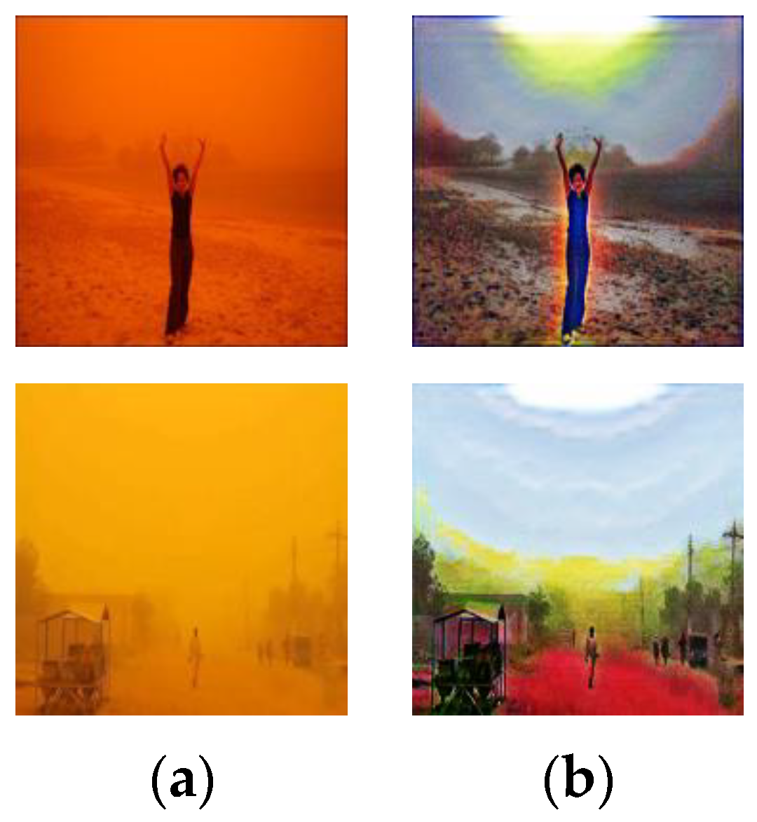
Generative adversarial networks (GANs) were originally proposed by Goodfellow et al. [15] and have achieved great success in the field of image generation. However, such networks still require paired datasets for training. Recently, Zhu et al. [16] proposed a cycle-consistent generative adversarial network (CycleGAN) for image translation problems. Two generators and two discriminators are proposed and combined with cyclic consistency loss to solve the unpaired training of images problem. Inspired by CycleGAN, we converted the image dedusting problem into an image translation problem. That is, the basic idea is to let the network learn the mapping relationship between the sand–dust domain and the clean domain and establish an unpaired mapping relationship between these two domains. This idea does not require paired datasets to be trained in an unsupervised way. Through training, the sand–dust domain can fit the distribution of the clean domain as much as possible to achieve the purpose of removing sand dust. Specifically, D-CycleGAN is proposed for image dedusting. Due to unsupervised learning, the solution space of the two domains is large and needs to be more constrained. We designed a jointly optimized guided module (JOGM) to limit the solution space of the network and make the mapping more accurate. To further improve the image quality, the proposed hidden layer adversarial branch was performed to reduce the chance of an erroneous propagation of the gradient information in the hidden layers of the network, thus improving the quality of image generation. Due to the lack of corresponding ground-truth clean image supervision, the proposed joint loss function can help network training and promote the generation of image details. The effect is shown in Figure 1.
The main contributions of this paper are as follows:
- (1)
- The D-CycleGAN is the first work that successfully introduces unpaired training to sand-dust image restoration. This work eliminates the dependence on paired data and does not require the estimation of any physical model parameters and can be well generalized to realistic applications;
- (2)
- We propose a jointly optimized guided module (JOGM) and a hidden layer adversarial branch to constrain the network model from the outside and inside of the network, which can improve the quality of the generated image;
- (3)
- Experiments demonstrate that the proposed method exhibits better image quality and outperforms other advanced comparison algorithms. We also contribute sand-dust datasets including some aerial sand-dust datasets to promote research in the field of sand-dust images.
2. Related Work
In this section, we evaluate the research progress of image dedusting from two aspects. One is based on traditional image dedusting methods, and the other is based on learning methods. Since there are relatively few studies on learning-based image dedusting, we mainly review the relevant progress in the field of image dehazing.
2.1. Traditional Image Dedusting Methods
Al-Ameen [4] proposed a fuzzy operator for the sand-dust image enhancement algorithm. First, the three channels of the sand-dust image are linearly stretched to correct the color, and then the fuzzy subordinate function is applied to the three channels to enhance the image details. The color correction of this method does not consider the characteristics of the sand-dust images, and the effect is not ideal. Xu et al. [5] proposed a least-squares model for sand-dust images. Park et al. [6] proposed successive color balance sand-dust image enhancements with coincident chromaticity histograms. The method removes color shifts effectively and enhances details in the distance, though a large amount of noise appears in the image. Similar image-based enhancement methods are also available in the literature [17,18,19,20], which enhance a sand-dust image to different degrees, though they affect the subjective effect due to overenhancement. Atmospheric scattering model-based methods require the estimation of some physical parameters and specific priors to recover images more effectively. The dark channel prior proposed by He et al. [21] has been widely used and promoted in image dehazing, however, this prior is not applicable to image dedusting. Peng et al. [22] improved the dark channel and proposed a more generalized dark channel prior and incorporated an adaptive color correction model into the image formation model to recover various degraded images, though the algorithm was not effective in removing the color shift from sand-dust images. Yang et al. [7] used histogram matching for color correction of sand-dust images and developed an atmospheric scattering model with Gaussian adaptive transmission maps to recover image details, though the details recovered from the sky are prone to halos. Gao et al. [8] proposed a method of reversing the blue channel prior for sand-dust image restoration, which can effectively remove sand dust, though it is prone to color distortion when dealing with severe sand-dust images. Shi et al. [9] proposed a halo-reduced sand-dust image restoration method by implementing color correction in a lab space, removing haze by applying a halo-reduced dark channel prior, and then using contrast-limited adaptive histograms equalization (CLAHE) to enhance the contrast. However, this method causes the image to be overenhanced, and the overall tone is cooler. Kim et al. [23] proposed saturation stretching to improve transmittance and remove the color shift using a white balance technique. This color balance technique does not take into account the characteristics of the sand-dust images, resulting in blue artifacts in the images. Dhara et al. [24] proposed optimizing the dark channel by using weighted least squares filtering to obtain the transmission map and removing the color shift by adaptive atmospheric light. Although the algorithm enhances the details of the image, the image has serious distortion problems. Bartani et al. [25] proposed an adaptive optical physical sand-dust removal method using optimized air light and a transfer function. However, the method could not handle severe sand-dust images. The traditional methods have achieved certain results in image dedusting, though there are still various problems in the process of image restoration, such as image overenhancement, color distortion, and noise.
2.2. Learning-Based Methods
Recently, convolutional neural networks and generative adversarial networks have gained much attention in the research community and have achieved great success in the field of image restoration. Cai et al. [26] proposed DehazeNet, which is used to estimate the transmission map by designing a nonlinear activation function and feature extraction unit. Qin et al. [27] proposed an end-to-end feature fusion attention network that aggregates channel attention and pixel attention for better haze removal. Qu et al. [28] proposed an enhanced pix2pix dehazing network, which combines a generative adversarial network and an enhancer to jointly optimize the network, which has achieved good dehazing results. Although these learning-based methods have achieved good results in image dehazing, these methods require a large number of paired datasets, and it is difficult to obtain paired datasets for sand-dust images. Due to the complex physical causes of sand-dust image formation, the haze synthesis method is not suitable for sand dust. Recently, some researchers, such as Si et al. [29], tried to explore synthetic sand-dust images. Although they synthesized similar sand-dust images, there was still a certain gap between them and real sand-dust images. Huang et al. [13] also tried to establish a sand-dust image dataset and proposed SIDNet for image dedusting. However, from the perspective of the recovery effect of real sand-dust images, there is still color distortion and residual sand-dust. Huang et al. [14] proposed a feature fusion image dedusting network, though the application in real scenes is not ideal. Liang et al. [30] proposed a learnable dedusting network that first removes the color shift by color compensation and histogram equalization and then introduces three subnetworks of atmospheric light, transmission map, and clear image estimation layer to remove the haze effects. This method removes haze well, though it is prone to a distortion problem with yellowish colors. All these methods require a paired dataset approach for training until CycleGAN was proposed to solve the problem of training on unpaired datasets. CycleGAN is mainly used for translation between images, such as a horse to a zebra. Inspired by CycleGAN, Engin et al. [31] proposed introducing CycleGAN to the image dehazing task and combined it with perceptual loss to improve the image dehazing performance. Yang et al. [32] proposed a disentanglement dehazing network, which utilizes three generators to disentangle the parameters of the physical model. The network does not require paired data and is an unsupervised dehazing work. Liu et al. [33] proposed a two-stage mapping CycleGAN network for dehazing, which embeds prior knowledge to improve the dehazing performance and obtain a better dehazing effect. A great advantage of CycleGAN is that it does not require paired datasets, which forces us to remove sand dust from a new perspective, namely, an unsupervised method, to solve the difficulty in obtaining paired sand dust datasets. However, the original CycleGAN still has some shortcomings, such as artifacts and color artifacts, when applying image dedusting tasks. Therefore, based on the old CycleGAN, the new CycleGAN is introduced for the image dedusting task. We improved CycleGAN in two aspects. One is the network structure and the other is the loss function. The network structure of CycleGAN is improved from the inside and outside, and the image quality is promoted by imposing conditional constraints on the inside and outside of the network. The improved loss function promotes the generation of image details and the restoration of color information.
3. The Proposed Method
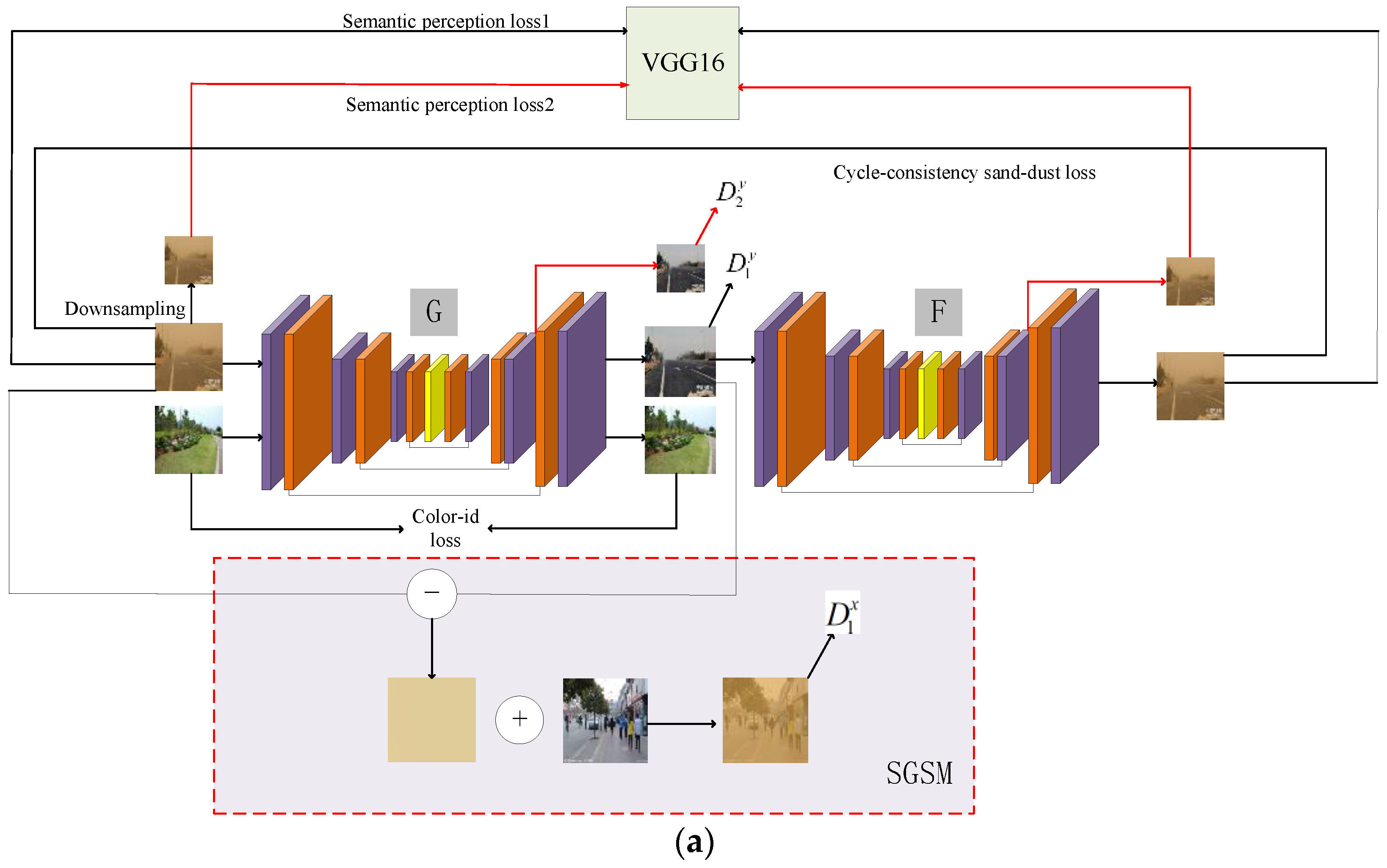
In this section, we mainly introduce the network structure of D-CycleGAN. We improve the original CycleGAN in three aspects, including the proposed joint optimization modules (SGSM and CGSM), the network hidden layer adversarial structure, the dual-scale semantic perception loss in the feature space, and the color identity-preserving loss function in pixel space. As shown in Figure 2, the network model includes two paths of the forward translation cycle and backward translation cycle, the cycle of sand image–clean image–sand image, and the cycle of clean image–sand image–clean image. Each generator has two outputs, both with two corresponding discriminators. The quality of image generation is improved by confronting the outputs of the two scales. Suppose the sand image set is , where and represents the number of sand images. The clean image set is , where , represents the number of clean images, is not necessarily equal to , and there is no one-to-one correspondence between and . Note that the clean images here are from outdoor real-scene images. The forward translation process is shown in Figure 2a, where the generator, , is responsible for learning the sand image domain to the clean domain so that the distribution of the sand image is as close as possible to the distribution of the clean image, i.e., . The generator, , is responsible for mapping the image generated by to the sand domain, i.e., , so that is close to , which ensures the correspondence in the translation process, and this process completes the forward translation process. The backward translation process is shown in Figure 2b, where the clean domain image is mapped by generator to a distribution close to the sand domain, i.e., , and then returned by generator to the clean domain, i.e., . Similarly, is equal to as much as possible. In the following, we will specify the details of the proposed network model. The structure of the proposed generator is presented in Section 3.1. The structure of the discriminator is given in Section 3.2. The details of the joint optimization module are presented in Section 3.3. The final objective function is given in Section 3.4.
3.1. Generator
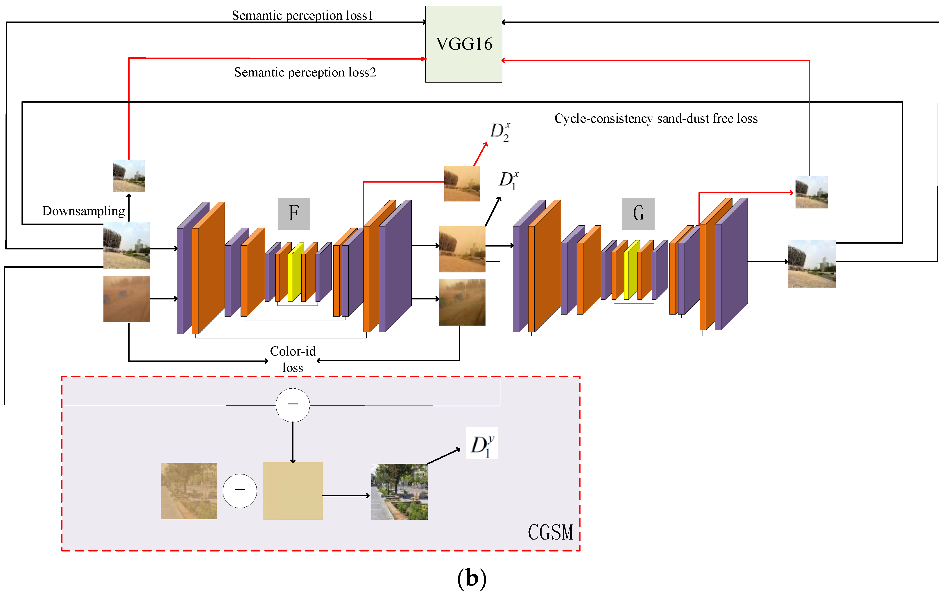
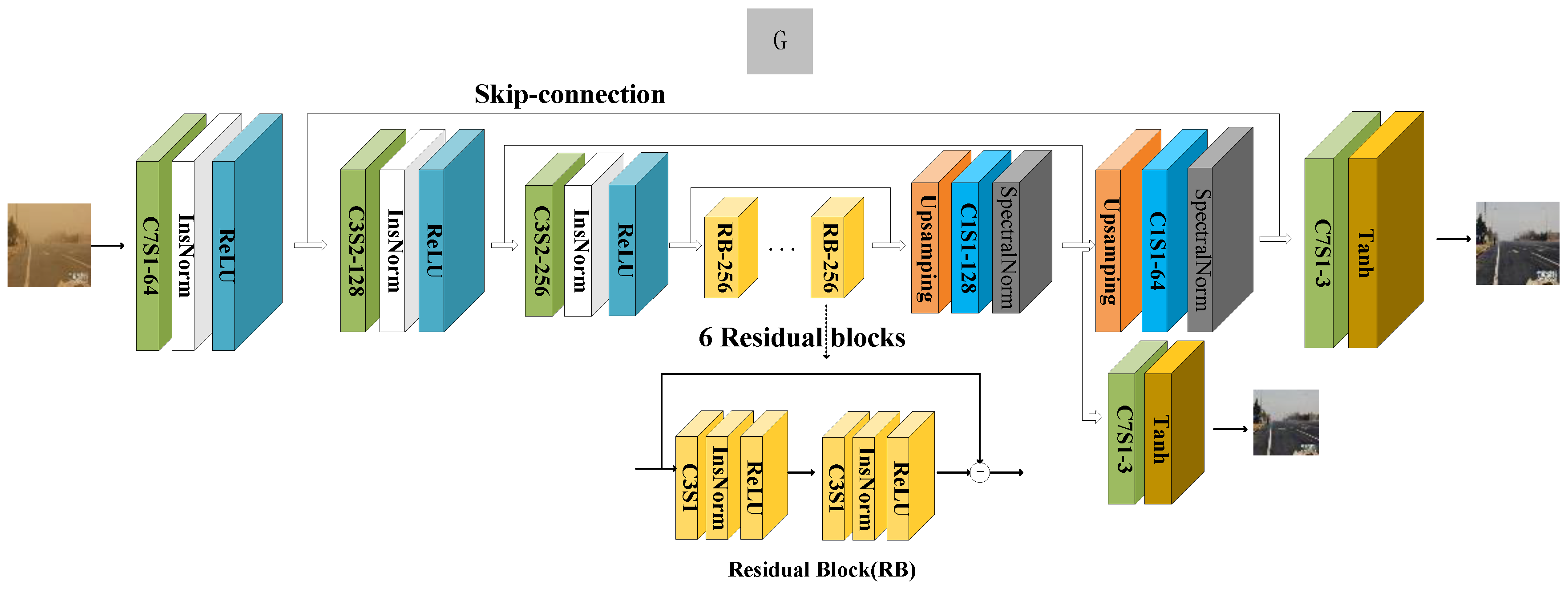
The proposed generator adopts an encoder–decoder structure similar to CycleGAN, including an encoding structure, a feature transformer, and a decoding part. Different from CycleGAN, to adapt to our image recovery task, we make full use of the low-level features and fuse the coding structure and decoding structure with the same resolution through skip connections to recover more details of the image. The generator structure is shown in Figure 3. In the encoding part, there are a convolutional layer, normalization function, InsNorm, and nonlinear function, ReLU, followed by two downsampling units. The feature transformer consists of six identical residual block units in a series. In the decoding part, the original CycleGAN adopts the deconvolution method for upsampling, though this upsampling method will cause a checkerboard effect on the image [34]. To reduce this effect, we use interpolation instead of deconvolution. The spectral normalization function was proposed by [35]. It has been proven that the network can be trained smoothly during training. The interpolation is followed by convolution and spectral normalization functions to perform feature enhancement and improve the stability of the network training. Note that the generators and have the same network structure. We not only output the adversarial at the end of the network but also propose the adversarial structure of the network. By performing the adversarial in the hidden layer, the generated real and fake images are discriminated, and the error of gradient propagation is reduced to better improve the quality of the image. Assume that the sand-dust image set is , where , denotes the number of sand-dust images and the clean image set is , where , denotes the number of images, and is not necessarily equal to . The forward translation process is expressed as follows:
where refers to an image in the domain, are the two output images of the generator , where the subscripts one and two of generators and denote the generator with network end structure and the generator with a hidden layer structure, respectively. Where is the output image at the end of the network and is the output image of the hidden layer. Here, for , we introduce two independent discriminators, and , to generate adversarial images to distinguish between the real and fake images, supervise from the end of the network, and supervise the hidden layer of the network , to reduce errors in the propagation of the gradient information in the hidden layer of the network and to improve the quality of . We only take as the input of the generator , and are the reconstructed images, respectively; is the output of the end of the network and is the output of the hidden layer of the network. Similarly, the backward translation process, i.e., clean–sand–clean, can be expressed as follows:
where refers to an image in the domain, are the two output images of the generator , where is the output image at the end of the network and is the output image of the hidden layer. Here, for , two independent discriminators, are introduced to generate adversarial responses to constrain the output of .
3.2. Discriminator
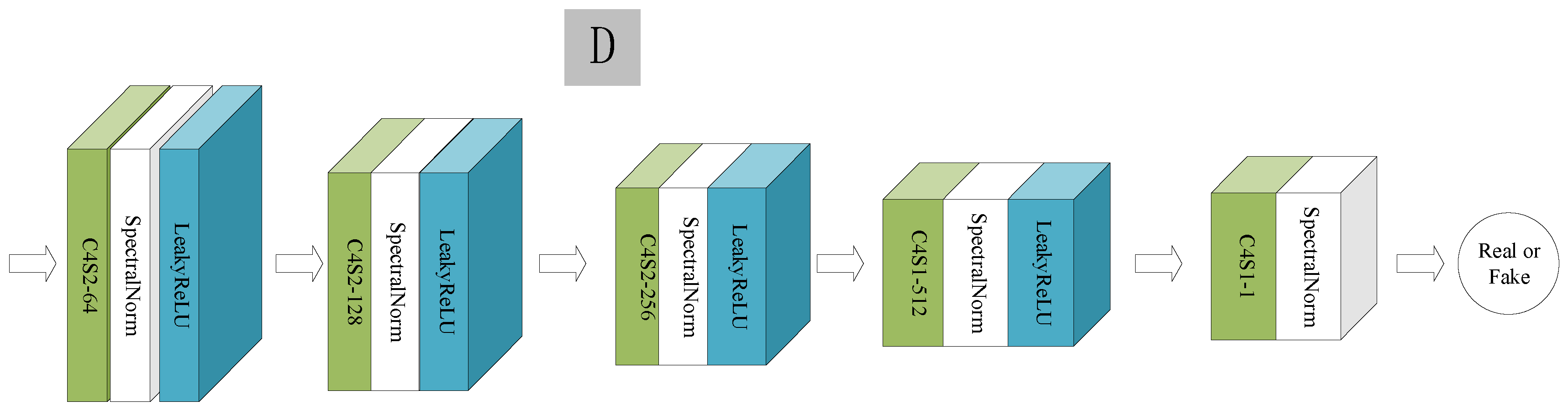
The main role of the discriminator is to distinguish between real images and fake images and guide the generator through a continuous confrontation with the generator. Some generative adversarial networks, such as GAN-based dehazing methods [31,36], use a single discriminator to supervise the end of the network, though when encountering haze with an uneven concentration, the ability of a single discriminator is limited and cannot effectively distinguish between certain haze regions. Therefore, to remove localized haze regions, Refs. [37,38] used two discriminators against different sizes of the end outputs of the network to improve the defogging performance. These methods are processed from the end output of the network and cannot supervise the hidden layer of the network, so their improved performance is limited. Unlike these methods, we not only counteract the end of the network but also introduce discriminators from the hidden layer of the network to reduce the error of gradient information propagation and better guide the generator. The discriminator we used is the base PatchGAN [16]. To train the discriminator stably, we introduce a spectral normalization function after each convolutional layer. The discriminators in the network model all have the same structure. The structure is shown in Figure 4, which consists of five convolutional layers, and the spectral normalization function is added after each convolution. LeakyReLU is the activation function. The output channels of each layer are 64, 128, 256, 512, and 1 in sequence, and the input image is judged true or false in the last dimension.
3.3. Joint Optimization Guidance Module
Due to unsupervised unpaired sand-dust image enhancement, lack of real image reference, and different degrees of the color shift in sand-dust images, the existing unsupervised framework does not effectively constrain the generator, resulting in the presence of sand-dust or some color distortion and halo artifacts in the image content. Therefore, to constrain the network more efficiently, we designed a jointly optimized guided module (JOGM), comprised of the sandy guided synthesis module (SGSM) and the clean guided synthesis module (CGSM). We introduced SGSM and CGSM in the forward translation and backward translation processes, respectively. Their structures are shown in Figure 2a,b. Specifically, we simply model the sand-dust image by considering that the sand-dust image consists of image clean content and color shift components, i.e., ; represents the sand-dust image, represents the image clean content, and is the color shift component. From Equation (1), represents the output at the end of the network, and we consider that the generated by the generator does not contain sand-dust components if it is good enough. Then, is only the color shift component, and the synthesized sand-dust image is more realistic. By feeding to the discriminator , and constantly confront each other and feedback the information to the generator, which leads the generator , to generate content images with no color shift so that the generator produces a better image quality. Note that here is the same discriminator as the discriminator mentioned in Section 3.1, and the weight parameters are shared because the discriminator here has the same function, which is to distinguish between the real sand-dust images and the generated sand-dust images. Similarly, the discriminator, , used in the CGSM mentioned below is also the same. To ensure stable training of the network, the LSGAN loss function [39] is utilized, where the guided adversarial loss is defined as:
where and are the losses of generator and discriminator , respectively. Similarly, in the backward translation process, we introduce CGSM. From Equation (3), the color shift component is , and the synthesized clean image is . By feeding into the discriminator, , to determine whether it is true or false, the generator is guided to improve so that is closer to the distribution of real sand-dust images. Generators and are complementary to each other. By jointly constraining the network by two guided synthesis modules, the space for generating the image solutions can be better limited, which is beneficial for improving the quality of the generator. Then, the clean image synthesis guided module loss is:
where and are the losses of generator and discriminator , respectively.
3.4. Loss Function
Loss functions play an important role in unsupervised networks, especially in unsupervised unpaired image tasks, where more efficient loss functions are needed for constraints. To recover the color information of the image, we propose a color identity-preserving loss in the pixel space that effectively preserves the inherent color information of the image. In the feature space, a dual-scale semantic perceptual loss is proposed to reduce the artifacts and recover more detailed information. Below, we give the details of several loss functions we specifically use.
Cycle consistency loss: To preserve the image detail information and texture information while reducing the contradiction between the generator and mapping, we introduce the cycle consistency loss in CycleGAN. Taking the forward translation process as an example, for each image from domain , the image translation cycle should be able to bring back to the original image, i.e., . The backward process is also similar, with . Then, the total cycle consistency loss is defined as:
where is the L1 norm loss, and the L1 norm loss is used to calculate the minimization of the reconstructed image and the input sand-dust image , so that is as close to as possible. Similarly, the backward translation process is as close as possible to .
Adversarial loss: Through adversarial training, the adversarial loss can gradually match the generated image data distribution to the data distribution in the target domain. Since our generator has two outputs with different resolutions at the end of the network and at the hidden layer, the corresponding two discriminators are confronted separately, so there are two adversarial losses. For generator , the corresponding discriminators are , and the generator loss is defined as:
represents the output of the hidden layer of generator . Similarly, for generator , the corresponding discriminators are , whose losses can be defined as:
where and are the guided losses mentioned in Section 3.3. Where refers to the output of the hidden layer of , the total loss of the corresponding generator is:
The losses of the corresponding discriminators are:
Then, the total loss of the discriminator is:
where and are the guided losses mentioned in Section 3.3.
Color identity preservation loss: The reconstruction of image details can be enhanced using cycle consistency loss, however, it is not sufficient to recover images using this loss alone since this loss does not effectively recover the color information inherent in the image. For this reason, we propose a color identity preserving loss in the pixel space, which can give the generator the ability to recover the image color information by constraining the generator. Specifically, as shown in Figure 2a, for example, when a sand-dust image , is fed to generator , it can convert the sand-dust image into a clear image. At the same time, when the clean domain image , is sent to the same generator , it can also output a clean image; that is, the output image is kept as much as possible as the input original image. This loss gives the generator the ability to restore, as much as possible, the color information that the image object itself contains. This color identity preservation loss is defined as:
where the first term on the right side indicates that, for the forward translation process, the generator can recover the clean image itself when a clean image is input. Similarly, for the backward translation process, when a sand-dust image is input, generator can also recover the sand-dust image itself.
Dual-scale semantic perceptual loss: Although the cycle consistency loss can help the generator learn some texture details, this loss is constrained in the pixel space and cannot effectively constrain the consistency of the cyclic image , and the original image , as well as the consistency of and . As a result, the perceived quality of the translated image is not very good, and there are often artifacts and unclear texture details. To improve the image quality, we compute feature distances in the feature space using a pretrained VGG-16 model [40] for the deep semantic features of the cyclic image and the original image to better preserve the texture details of the images. The proposed feature semantic perception is performed at two output scales, an output at the end of the network, and an output at the hidden layer. Ablation experiments demonstrate that applying the semantic perception function at both scales can better improve the quality of the images. Dual-scale semantic perception is defined as:
where is a VGG16 feature extractor from the second and fifth pooling layers, represents the -norm, and and , are half of the resolutions of and , respectively. The first two terms on the right side of the equation represent the semantic perceptual loss applied to the end of the network, and the last two terms of the equation represent the semantic perceptual loss to the hidden layer.
Finally, the total loss function for network model training is:
where , , and are used to balance the weights of different losses to emphasize their importance. Thus, the overall objective function of the GAN network is:
The discriminator and the generator are a mutual game process, where the goal of the generator is to minimize the target loss, while the discriminator is trying to maximize the objective function, and finally, both reach a stable state.
4. Experimental Results
4.1. Dataset and Application Details
Our network model does not require paired sand-dust image sets for training, which facilitates training of the network model. Since there are no large public datasets available for sand-dust images, in order to train the network model, we contributed datasets for sand research to promote the development of this field. We collected some clean domain images from the RESIDE dataset [41] since some of the images in the dataset are blurred and the quality is not high. We also collected clean domain images and sand-dust domain images from the internet. Among them, there are 700 sand-dust images in the training set and 3000 clean images in the training set. The test set includes 130 natural scene sand-dust images, which we call NSI. In addition, to explore the impact on remote sensing images, we also collected a small 30 aerial sand-dust images, which we call ASI. The test set and training set are not repeated. Since the collected images are of different sizes, we uniformly resized the images to 256 × 256 to facilitate the training of the network model, the images of the test set are also resized to 256 × 256, and the images are converted to png format for output.
Our network models are implemented in PyTorch, and all experiments are performed on an NVIDIA Tesla V100 GPU with 16 GB of memory. During training, we fix the discriminator and update the generator once, and then fix the generator and update the discriminator once, i.e., we alternately optimize the generator and discriminator. ADAM is used as an optimizer for model training with parameters of β1 = 0.9 and β2 = 0.999. The batch size is set to one. Our network is trained for a total of 200 epochs. For the first 100 epochs, the learning rate is set to 0.0002, and linear decay to zero for the next 100 epochs. The parameters of Formula (18) are empirically set as = 10, = 0.5, and = 1.
4.2. Ablation Studies
To demonstrate the effectiveness of the proposed module, the CycleGAN in Figure 2 is used as the base framework baseline, i.e., excluding our proposed hidden layer adversarial branch, jointly optimizing the guided module (SGSM and CGSM), and using the proposed hidden layer semantic feature loss. We highlight the main differences between the baseline and the proposed CycleGAN structure with red solid and red dashed boxes in Figure 2. On the basis of the baseline, the proposed components are gradually added to verify the impact of the proposed components on the network performance. Since sand-dust images do not correspond to ground-truth images, we cannot evaluate images with reference image metrics such as PSNR and SSIM. Here, we chose the nonreference image metrics spatial-spectral entropy-based quality SSEQ [42] and blind image quality indices BIQI [43] to evaluate the quality of the images on the test set NSI, both of which proved to be effective in evaluating the sand-dust images in the literature [29]. The smaller the SSEQ and BIQI values are, the higher the quality of the image. We performed five sets of experiments: (1) Baseline: the baseline mentioned above is noted as baseline; (2) Baseline+a: add the proposed SGSM on the basis of the baseline; (3) Baseline+b: add the proposed CGSM on the basis of the baseline; (4) Baseline+a+b: add the proposed SGSM and CGSM on the basis of the baseline; (5) Baseline+a+b+adv: add the hidden adversarial branch on the basis of (4); (6) Baseline+a+b+adv+ploss: add the hidden layer semantic perceptual loss on the basis of (5). The objective indicators are shown in Table 1.
From the objective metrics, the metric of Baseline+a is higher than that of the baseline, which indicates that the SGSM alone does not constrain the network well. Baseline+b has a lower metric than baseline, and SSEQ and BIQI decreased by 0.54 and 1.17, respectively, indicating that CGSM can improve the quality of images. However, through Baseline+a+b, it is found that the joint use of SGSM and CGSM has stronger constraints on the network and can better improve the image quality than the single use of SGSM or CGSM. SSEQ and BIQI decreased by 1.02 and 1.36 respectively compared to the baseline, which proves the effectiveness of the jointly optimized guided module. After adding the hidden adversarial branch, the metrics SSEQ and BIQI decreased from 13.56 and 19.70 to 13.50 and 19.62, respectively, and the quality of the images was further improved, which proved the effectiveness of the hidden adversarial branch. Finally, based on the previous component, we added the hidden layer semantic perception loss. The metrics SSEQ and BIQI decreased by 0.09 and 0.12, respectively, proving the effectiveness of the semantic perception loss.
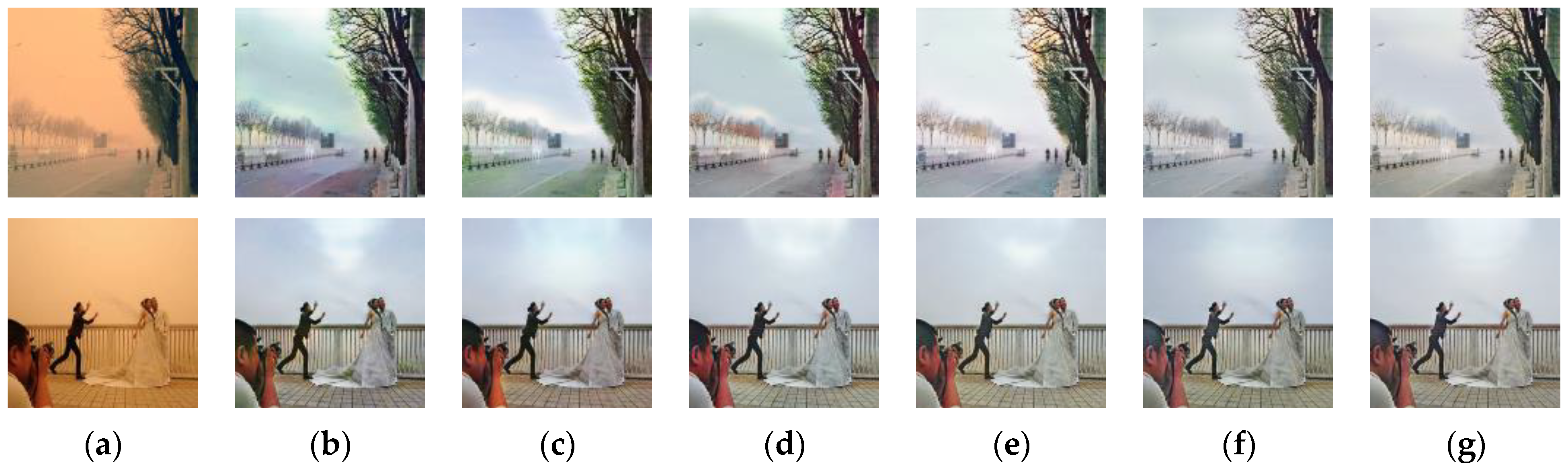
In addition, we also present the subjective effects of the ablation experiments, as shown in Figure 5. For the convenience of analysis, we recorded the picture in the first row as “street” and the picture in the second row as “people”. From Figure 5b, it can be seen that when the proposed components are not added, the color shift is removed from the baseline, the overall quality of the image is not high and there are still color artifacts and halos in the image, such as in “street”; its roads and sky are distorted in color, and the trees have halos. In “people”, the skirts and guardrails have color distortion, and there is a halo problem in the sky. Figure 5c,d improve the image quality to some extent, and the effect is limited. In contrast to Figure 5c,d, the joint module used in Figure 5e can significantly improve the image quality, and the halo and color distortion in the image are significantly improved. Figure 5f,g further reduce the halo and make the image more natural. This subjective effect also proves the effectiveness of the proposed components.
To verify the effectiveness of the proposed color identity preservation loss and the dual-scale semantic perceptual loss, we performed the following ablation experiments: (1) no vgg: the other components of the network remain unchanged, and only the dual-scale semantic perceptual loss of the feature space is removed; (2) no color: the other components of the network remain unchanged, and only the color identity preservation loss is removed; (3) ours: the completed network model. Table 2 gives the average SSEQ and BIQI scores for the different loss functions.
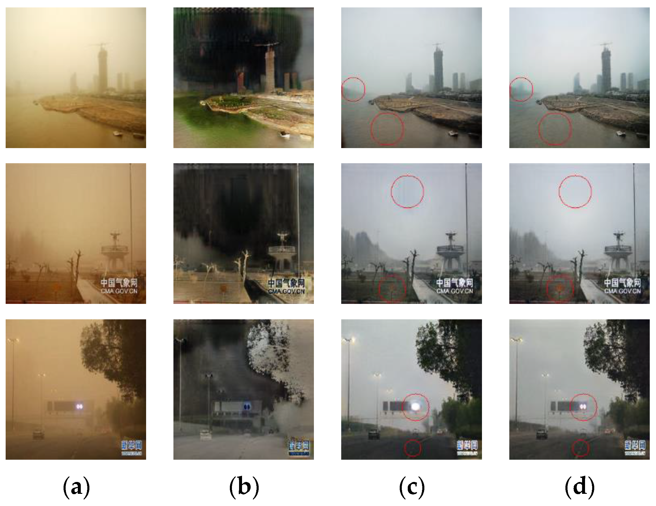
Table 2 shows that, compared with the complete network model, the average scores of SSEQ and BIQI increased by 1.55 and 0.1, respectively, when there was no dual-scale semantic perception loss. When there was no loss of color identity preservation, the average SSEQ and BIQI scores increased by 2.68 and 2.54, respectively. The effectiveness of the proposed loss function is proved. Meanwhile, from the influence degree of the loss function, the proposed color identity preservation loss has an important influence on the quality of the image. From the subjective effect of Figure 6b, we can also see that, without the loss of color identity preservation, the inherent color of the image will not be recovered, the image will appear gray and white as a whole, and the image quality will be seriously degraded. As seen in Figure 6c, when there is no dual-scale semantic perception function, the image will not be able to enhance the details in the distance, and the image will have artifacts and unclear details, as detailed in the red circles in the image.
4.3. Qualitative and Quantitative Evaluation
To demonstrate the superiority of the proposed model, we qualitatively and quantitatively compared it with nine other sand-dust comparison algorithms, TF [4], GDCP [22], RDCP [9], CC [24], FSS [23], VR [7], RBCP [8], SES [6], and AOP [25] on test sets NSI and ASI. The source code of the comparison algorithm comes from the website published by the author.
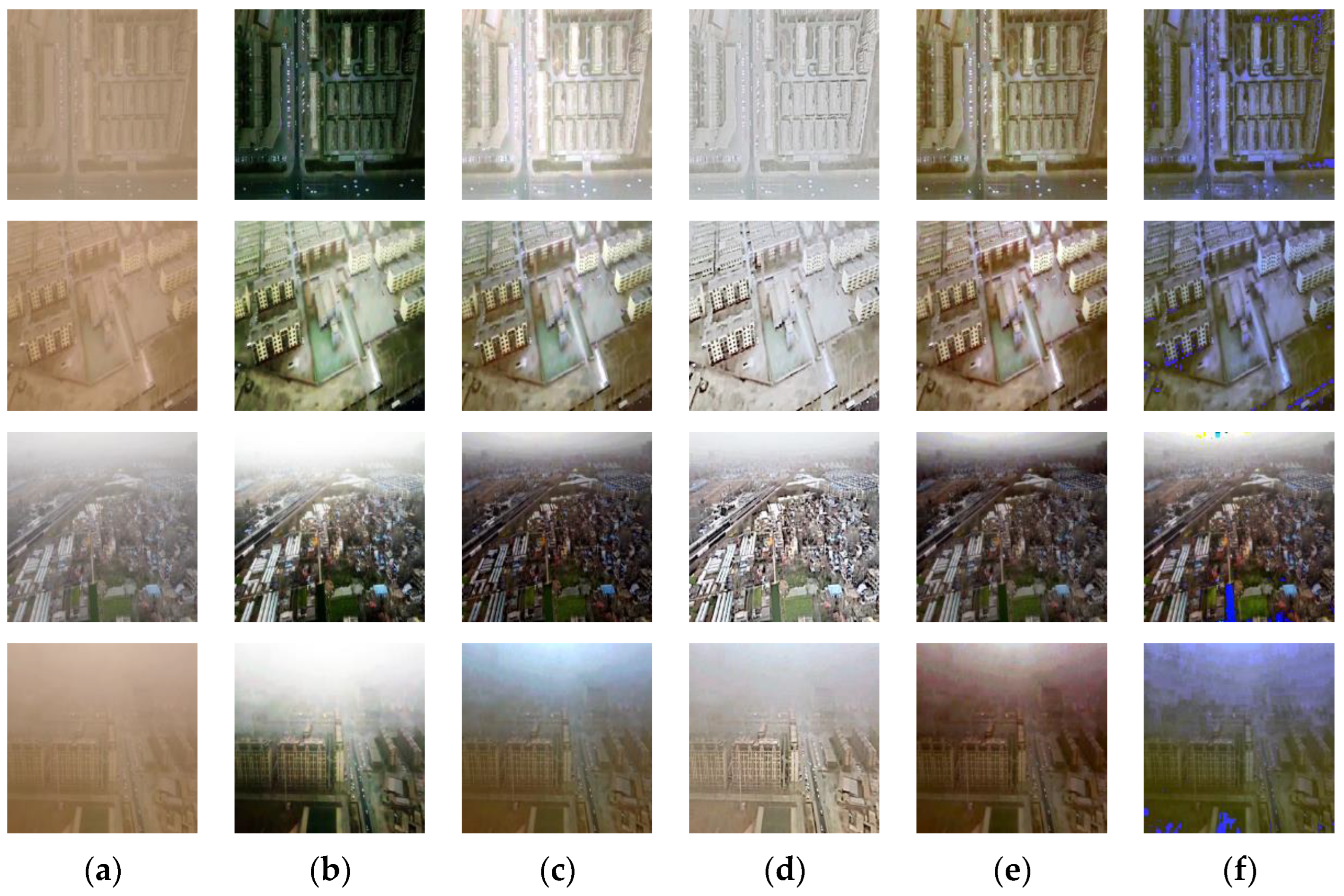
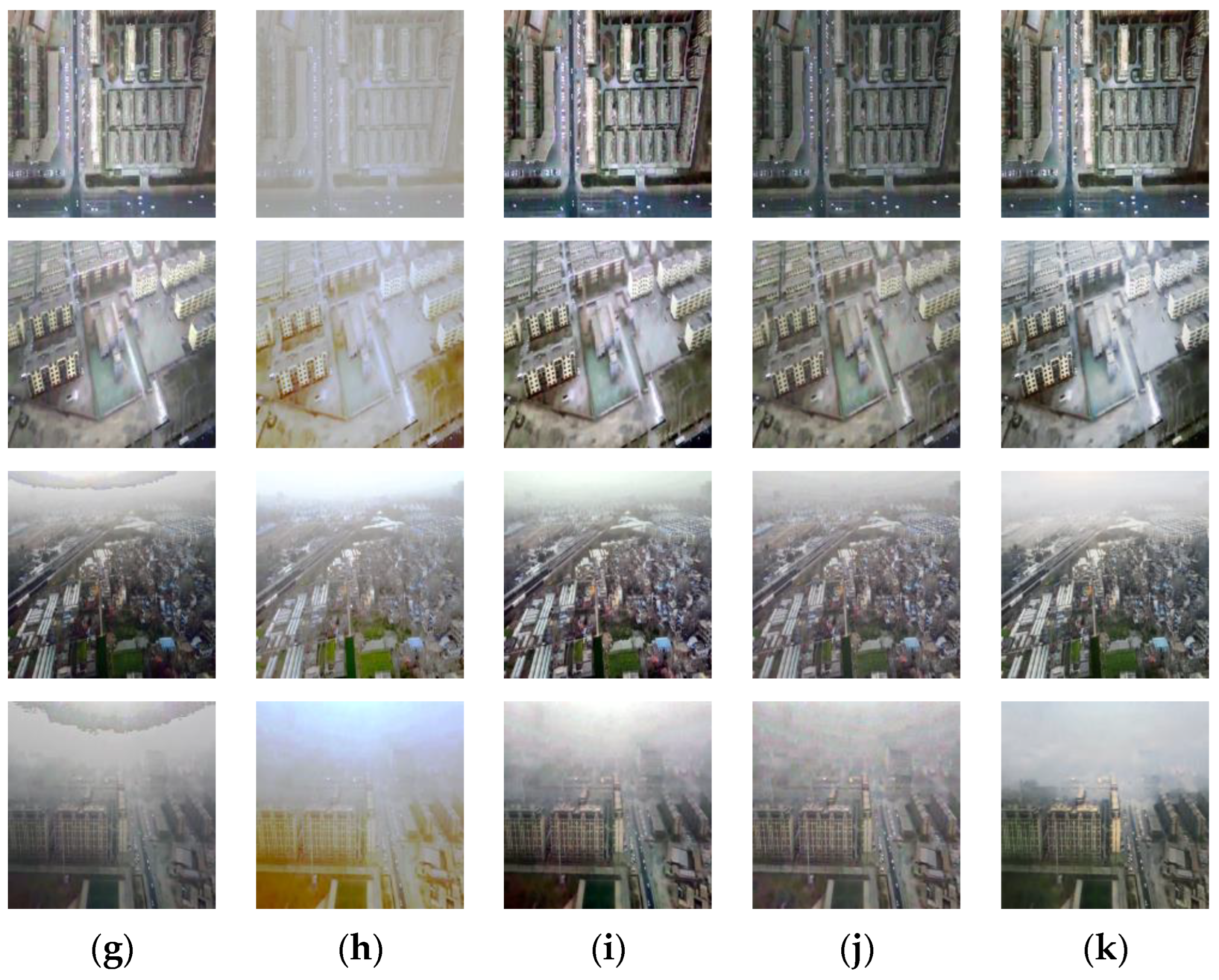
Qualitative Results. From Figure 7, when processing aerial sand-dust images, TF, GDCP, CC, and FSS have obvious color distortion and the overall effect is not good. RDCP, VR, RBCP, and AOP recover images with blurred details, and VR has obvious halos. SES recovers better details but causes slight color distortion and noise problems. Compared with other algorithms, the proposed algorithm has clear details and good visibility.
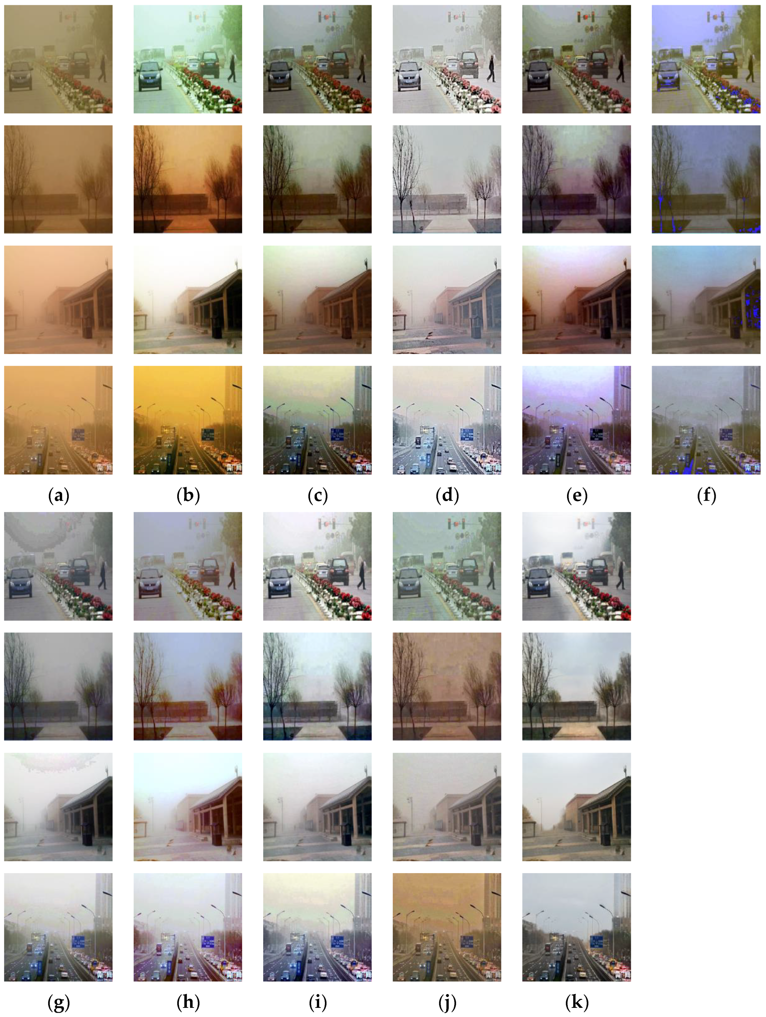
As seen from Figure 8, when processing natural scene sand-dust images, GDCP, CC, and FSS have poor recovery effects, and there is a color distortion phenomenon. The robustness of the algorithms of TF and AOP are not strong, it is difficult to remove the color shift for some images, and the processing effect is not ideal. The details recovered by VR and RBCP are not clear enough. In the VR method, there is still a halo phenomenon in the sky area, and in the RBCP method, there is also the problem of color distortion. RDCP removes the color shift well, though the overall image is cold. SES obtained relatively good visual effects, however, it can be seen from the restored effect that this method brings a large amount of noise in the process of enhancement, especially in the sky area. Compared with the other algorithms, the proposed method recovers clear details and has a higher image quality with less noise.
Quantitative Results. To more comprehensively evaluate sand-dust images, in addition to the SSEQ and BIQI metrics, we added other image nonreference indicator—the perception-based image quality evaluator PIQUE [44]. The lower the value of the indicator, the better the quality of the image. The quantitative results in the test sets ASI and NSI are given in Table 3 and Table 4, respectively. From the tables, the proposed algorithm outperforms the other comparison algorithms in all indicators except the indicator SSEQ of RDCP. In particular, RDCP leads to better indicator SSEQ than the proposed algorithm due to overenhancement, though the overall visibility is not good. Through quantitative and qualitative comparison, the proposed method has better comprehensive performance.
4.4. Run Time
To verify the performance of the algorithm, we give the running time of different comparison algorithms. In the comparison algorithms, different programming languages are used in the source code, where SES and FSS are written in Python language, our method run in PyTorch, and several other comparison algorithms are written in MATLAB language. To be fair, all methods are executed on a computer with an Intel(R) Core(TM) i7-8700 CPU @ 3.20 GHz, 16 GB RAM, and we also give the running time of the proposed method on a GPU with an NVIDIA Tesla V100 GPU and 16 GB RAM hardware conditions, and the results are shown in Table 5. The average time here is obtained by averaging over multiple runs of the test set NSI.
As seen from Table 5, except for the method RDCP, most of the traditional-based methods have relatively fast running times, however, their recovered results are not as good as ours. Additionally, we can also see that the proposed method has the fastest running speed when running on the GPU, which is nearly 14 times faster than that on the CPU.
4.5. Other Applications
4.5.1. Application One: Application in Image Dehazing and Underwater Image Enhancement
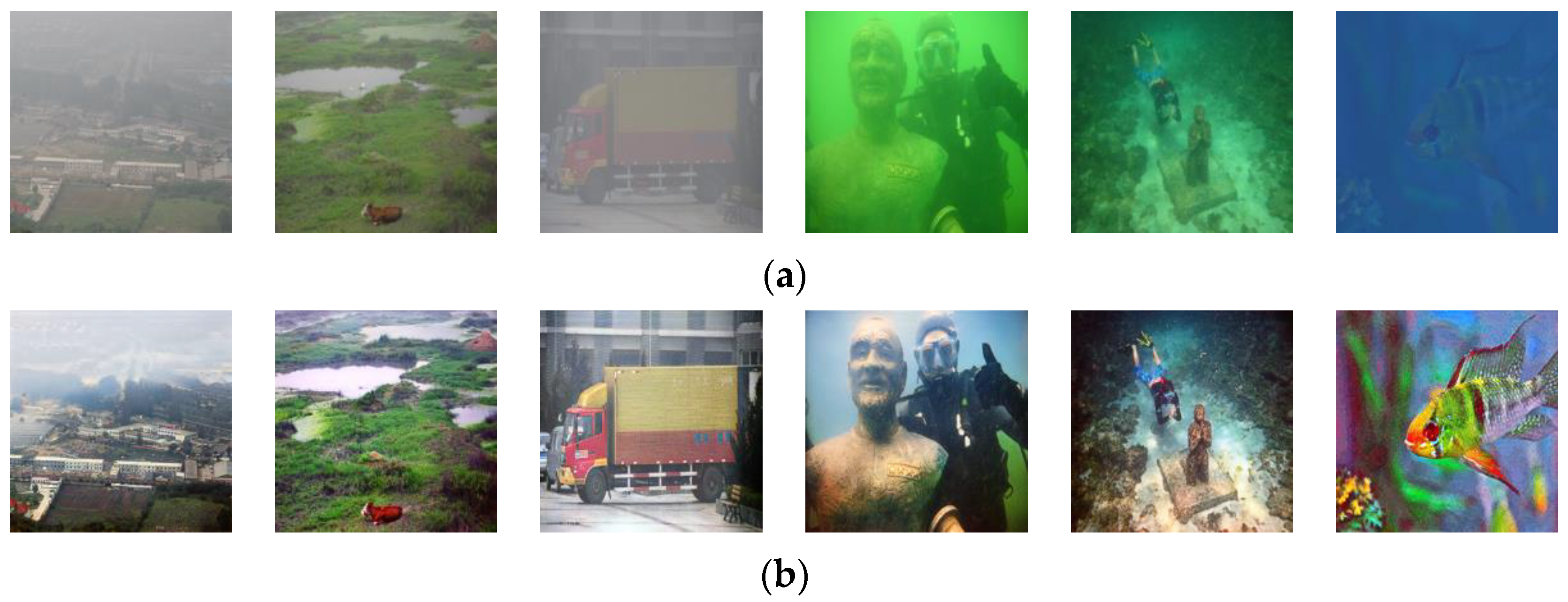
Although the proposed method is mainly for sand-dust image restoration, we find that the proposed method can also be generalized to other degraded images, such as haze and turbid underwater images. From Figure 9, we can observe that the proposed method recovers images with clear details and achieves satisfactory results on these degraded images.
4.5.2. Application Two: Application in Object Detection
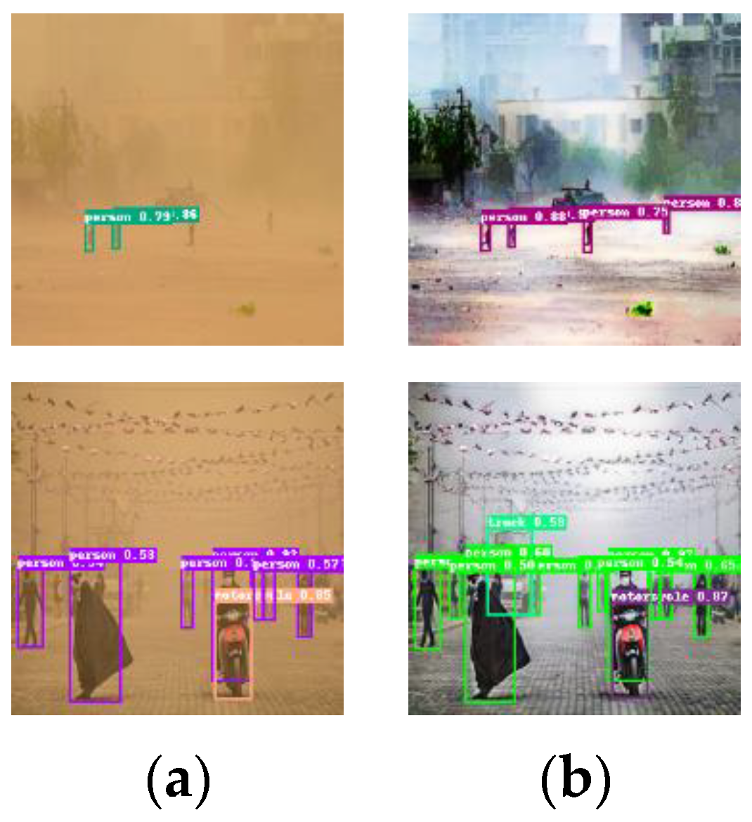
Object detection tasks have high requirements for image quality, and low-quality images seriously affect the accuracy and capabilities of object detection. Here, the PP-YOLO object detection algorithm proposed by Long et al. [45] is used for verification. As seen from Figure 10, in the first row, before processing, the detection accuracies of the four people in the image are 0.79, 0.86, 0, and 0, respectively. After processing, the detection accuracies of the proposed method are 0.88, 0.90, 0.75, and 0.80, respectively. Obviously, the proposed method improves the accuracy of detection, and the two people who were missed can be detected. In the second row, the proposed algorithm detects the truck and more people who were not detected originally after processing by the proposed algorithm. Since there are more objects in the second row, to illustrate the change in detection accuracy, we give the detection accuracy of the person standing in the foreground and the motorcycle. The accuracies of the person and motorcycle after processing by the proposed algorithm changed from 0.53 and 0.85 to 0.59 and 0.87, respectively. This shows that the proposed algorithm recovers more details and improves the quality of the image, which has an important impact on the advanced task of object detection.
4.6. Failure Cases
The proposed method cannot handle some severe sand-dust images. As shown in Figure 11, the processed images show halo and color distortion. The reason is that the sand-dust images are severely degraded, coupled with the fact that unsupervised network learning is used. The existing network constraints cannot effectively learn the characteristics of such images, resulting in poor recovery.
5. Conclusions
In this paper, we proposed an unsupervised network, D-CycleGAN, for image dedusting, which does not require paired images for training and solves the problem of the difficult acquisition of sand-dust paired datasets. A joint optimization module, including SGSM and CGSM, is designed to jointly guide the image generation, which significantly reduced the artifacts and color distortions. We reduced the error of the gradient information propagation by adding a hidden adversarial branch in the hidden layer of the network and further improve the quality of the image. The designed dual-scale semantic perceptual loss function and color identity preservation loss function better constrain the network model and facilitate the generation of detailed image information and image color information. Experiments show that, compared with other algorithms, the proposed method had high definition and image quality and achieved satisfactory visual effects, outperforming the other state-of-the-art algorithms. In addition, the proposed method generalized well to other low-level tasks, such as image dehazing and underwater image enhancement, and also facilitated the application of target detection.
Author Contributions
G.G.: Methodology, Validation, Writing—original draft. H.L.: Writing—review & editing. Z.J.: Funding acquisition. All authors have read and agreed to the published version of the manuscript.
Funding
This study is supported by the Natural Science Foundation of China (Grant Nos. U1903213 and U1803261) and Xinjiang University Innovation Project (XJU2022BS071).
Data Availability Statement
Data presented in this study are available upon request from the corresponding author.
Conflicts of Interest
The authors declare no conflict of interest.
References
- Kim, J.U.; Park, S.; Ro, Y.M. Robust small-scale pedestrian detection with cued recall via memory learning. In Proceedings of the IEEE/CVF International Conference on Computer Vision, Montreal, BC, Canada, 17 October 2021; pp. 3050–3059. [Google Scholar]
- Lamssaggad, A.; Benamar, N.; Hafid, A.S.; Msahli, M. A survey on the current security landscape of intelligent transportation systems. IEEE Access. 2021, 9, 9180–9208. [Google Scholar] [CrossRef]
- Alam, A.; Praveen, S.; Ahamad, F. Automatic Driving System by Recognizing Road Signs Using Digital Image Processing. In Computer Vision and Robotics; Springer: Berlin/Heidelberg, Germany, 2022; pp. 329–339. [Google Scholar]
- Al-Ameen, Z. Visibility enhancement for images captured in dusty weather via tuned tri-threshold fuzzy intensification operators. Int. J. Intell. Syst. Appl. 2016, 8, 10–17. [Google Scholar] [CrossRef] [Green Version]
- Xu, G.; Wang, X.; Xu, X. Single image enhancement in sandstorm weather via tensor least square. IEEE/CAA J. Autom. Sin. 2020, 7, 1649–1661. [Google Scholar] [CrossRef]
- Park, T.H.; Eom, I.K. Sand-dust image enhancement using successive color balance with coincident chromatic histogram. IEEE Access 2021, 9, 19749–19760. [Google Scholar] [CrossRef]
- Yang, Y.; Zhang, C.; Liu, L.; Chen, G.; Yue, H. Visibility restoration of single image captured in dust and haze weather conditions. Multidimens. Syst. Signal Process. 2020, 31, 619–633. [Google Scholar] [CrossRef]
- Gao, G.; Lai, H.; Jia, Z.; Liu, Y.; Wang, Y. Sand-Dust Image Restoration Based on Reversing the Blue Channel Prior. IEEE Photonics J. 2020, 12, 3900216. [Google Scholar] [CrossRef]
- Shi, Z.; Feng, Y.; Zhao, M.; Zhang, E.; He, L. Let You See in Sand Dust Weather: A Method Based on Halo-Reduced Dark Channel Prior Dehazing for Sand-Dust Image Enhancement. IEEE Access 2019, 7, 116722–116733. [Google Scholar] [CrossRef]
- Yu, J.; Liang, D.; Hang, B.; Gao, H. Aerial Image Dehazing Using Reinforcement Learning. Remote Sens. 2022, 14, 5998. [Google Scholar] [CrossRef]
- Lu, Z.; Li, J.; Liu, H.; Huang, C.; Zhang, L.; Zeng, T. Transformer for single image super-resolution. In Proceedings of the IEEE/CVF Conference on Computer Vision and Pattern Recognition, New Orleans, LA, USA, 24 June 2022; pp. 457–466. [Google Scholar]
- Zhang, Y.; Zhang, J.; Huang, B.; Fang, Z. Single-image deraining via a recurrent memory unit network. Knowl. Based Syst. 2021, 218, 106832. [Google Scholar] [CrossRef]
- Huang, J.; Xu, H.; Liu, G.; Wang, C.; Hu, Z.; Li, Z. SIDNet: A Single Image Dedusting Network with Color Cast Correction. Signal Process. 2022, 199, 108612. [Google Scholar] [CrossRef]
- Huang, J.; Li, Z.; Wang, C.; Yu, Z.; Cao, X. FFNet: A simple image dedusting network with feature fusion. Concurr. Comput. Pract. Exp. 2021, 33, e6462. [Google Scholar] [CrossRef]
- Goodfellow, I.; Pouget-Abadie, J.; Mirza, M.; Xu, B.; Warde-Far, D.; Ozai, S.; Courville, A.; Bengio, Y. Generative adversarial nets. Adv. Neural Inf. Process. Syst. 2014, 27. [Google Scholar] [CrossRef]
- Zhu, J.Y.; Park, T.; Isola, P.; Efros, A.A. Unpaired image-to-image translation using cycle-consistent adversarial networks. In Proceedings of the IEEE International Conference on Computer Vision, Venice, Italy, 22–29 October 2017; pp. 2223–2232. [Google Scholar]
- Cheng, Y.; Jia, Z.; Lai, H.; Yang, J.; Kasabov, N.K. A fast sand-dust image enhancement algorithm by blue channel compensation and guided image filtering. IEEE Access. 2020, 8, 196690–196699. [Google Scholar] [CrossRef]
- Wang, B.; Wei, B.; Kang, Z.; Hu, L.; Li, C. Fast color balance and multi-path fusion for sandstorm image enhancement. Signal Image Video Process. 2021, 15, 637–644. [Google Scholar] [CrossRef]
- Fu, X.; Huang, Y.; Zeng, D.; Zhang, X.P.; Ding, X. A fusion-based enhancing approach for single sandstorm image. In Proceedings of the 2014 IEEE 16th International Workshop on Multimedia Signal Process (MMSP), Jakarta, Indonesia, 22–24 September 2014; pp. 1–5. [Google Scholar]
- Gao, G.X.; Lai, H.C.; Liu, Y.Q.; Wang, L.J.; Jia, Z.H. Sandstorm image enhancement based on YUV space. Optik 2021, 226, 165659. [Google Scholar] [CrossRef]
- He, K.; Sun, J.; Tang, X. Single Image Haze Removal Using Dark Channel Prior. IEEE Trans. Pattern Anal. Mach. Intell. 2011, 33, 2341–2353. [Google Scholar]
- Peng, Y.T.; Cao, K.; Cosman, P.C. Generalization of the Dark Channel Prior for Single Image Restoration. IEEE Trans. Image Process. 2018, 27, 2856–2868. [Google Scholar] [CrossRef]
- Kim, S.E.; Park, T.H.; Eom, I.K. Fast Single Image Dehazing Using Saturation Based Transmission Map Estimation. IEEE Trans. Image Process. 2020, 29, 1985–1998. [Google Scholar] [CrossRef]
- Dhara, S.K.; Roy, M.; Sen, D.; Biswas, P.K. Color Cast Dependent Image Dehazing via Adaptive Airlight Refinement and Non-linear Color Balancing. IEEE Trans. Circuits Syst. Video Technol. 2020, 31, 2076–2081. [Google Scholar] [CrossRef]
- Bartani, A.; Abdollahpouri, A.; Ramezani, M.; Tab, F.A. An adaptive optic-physic based dust removal method using optimized air-light and transfer function. Multimed. Tools Appl. 2022, 81, 33823–33849. [Google Scholar] [CrossRef]
- Cai, B.; Xu, X.; Jia, K.; Qing, C.; Tao, D. Dehazenet: An end-to-end system for single image haze removal. IEEE Trans. Image Process. 2016, 25, 5187–5198. [Google Scholar] [CrossRef] [Green Version]
- Qin, X.; Wang, Z.; Bai, Y.; Xie, X.; Jia, H. FFA-Net: Feature fusion attention network for single image dehazing. In Proceedings of the AAAI Conference on Artificial Intelligence, New York, NY, USA, 7–12 February 2020; pp. 11908–11915. [Google Scholar]
- Qu, Y.; Chen, Y.; Huang, J.; Xie, Y. Enhanced pix2pix dehazing network. In Proceedings of the IEEE/CVF Conference on Computer Vision and Pattern Recognition, Long Beach, CA, USA, 15–20 June 2019; pp. 8160–8168. [Google Scholar]
- Si, Y.; Yang, F.; Guo, Y.; Zhang, W.; Yang, Y. A comprehensive benchmark analysis for sand dust image reconstruction. J. Vis. Commun. Image Represent. 2022, 89, 103638. [Google Scholar] [CrossRef]
- Liang, P.; Dong, P.; Wang, F.; Ma, P.; Bai, J.; Wang, B.; Li, C. Learning to remove sandstorm for image enhancement. Vis. Comput. 2022, 1–22. [Google Scholar] [CrossRef]
- Engin, D.; Genç, A.; Kemal Ekenel, H. Cycle-dehaze: Enhanced cyclegan for single image dehazing. In Proceedings of the IEEE Conference on Computer Vision and Pattern Recognition Workshops, Salt Lake City, UT, USA, 18–22 June 2018; pp. 825–833. [Google Scholar]
- Yang, X.; Xu, Z.; Luo, J. Towards perceptual image dehazing by physics-based disentanglement and adversarial training. In Proceedings of the AAAI Conference on Artificial Intelligence, New Orleans, LA, USA, 2–7 February 2018; p. 32. [Google Scholar]
- Liu, W.; Hou, X.; Duan, J.; Qiu, G. End-to-end single image fog removal using enhanced cycle consistent adversarial networks. IEEE Trans. Image Process. 2020, 29, 7819–7833. [Google Scholar] [CrossRef]
- Osakabe, T.; Tanaka, M.; Kinoshita, Y.; Kiya, H. CycleGAN without checkerboard artifacts for counter-forensics of fake-image detection. In International Workshop on Advanced Imaging Technology (IWAIT); SPIE: Bellingham, WA, USA, 2021; pp. 51–55. [Google Scholar]
- Miyato, T.; Kataoka, T.; Koyama, M.; Yoshida, Y. Spectral normalization for generative adversarial networks. arXiv 2018, arXiv:180205957. [Google Scholar]
- Chaitanya, B.; Mukherjee, S. Single image dehazing using improved cycleGAN. J. Vis. Commun. Image Represent. 2021, 74, 103014. [Google Scholar] [CrossRef]
- Zhao, J.; Zhang, J.; Li, Z.; Hwang, J.N.; Gao, Y.; Fang, Z.; Jiang, X.; Huang, B. Dd-cyclegan: Unpaired image dehazing via double-discriminator cycle-consistent generative adversarial network. Eng. Appl. Artif. Intell. 2019, 82, 263–271. [Google Scholar] [CrossRef]
- Mo, Y.; Li, C.; Zheng, Y.; Wu, X. DCA-CycleGAN: Unsupervised single image dehazing using Dark Channel Attention optimized CycleGAN. J. Vis. Commun. Image Represent. 2022, 82, 103431. [Google Scholar] [CrossRef]
- Mao, X.; Li, Q.; Xie, H.; Lau, R.Y.K.; Wang, Z.; Paul Smolley, S. Least squares generative adversarial networks. In Proceedings of the IEEE International Conference on Computer Vision, Venice, Italy, 22–29 October 2017; pp. 2794–2802. [Google Scholar]
- Simonyan, K.; Zisserman, A. Very deep convolutional networks for large-scale image recognition. arXiv 2014, arXiv:14091556. [Google Scholar]
- Li, B.; Ren, W.; Fu, D.; Tao, D.; Feng, D.; Zeng, W.; Wang, Z. Benchmarking Single-Image Dehazing and Beyond. IEEE Trans. Image Process. 2018, 28, 492–505. [Google Scholar] [CrossRef] [Green Version]
- Liu, L.; Liu, B.; Huang, H.; Bovik, A.C. No-reference image quality assessment based on spatial and spectral entropies. Signal Process. Image Commun. 2014, 29, 856–863. [Google Scholar] [CrossRef]
- Moorthy, A.K.; Bovik, A.C. A modular framework for constructing blind universal quality indices. IEEE Signal Process. Lett. 2009, 17, 7. [Google Scholar]
- Venkatanath, N.; Praneeth, D.; Bh, M.C.; Channappayya, S.S.; Medasani, S.S. Blind image quality evaluation using perception based features. In Proceedings of the 2015 Twenty First National Conference on Communications (NCC), Mumbai, India, 27 February–1 March 2015; pp. 1–6. [Google Scholar]
- Long, X.; Deng, K.; Wang, G.; Zhang, Y.; Dang, Q.; Gao, Y.; Shen, H.; Ren, J.; Han, S.; Ding, E.; et al. PP-YOLO: An effective and efficient implementation of object detector. arXiv 2020, arXiv:200712099. [Google Scholar]
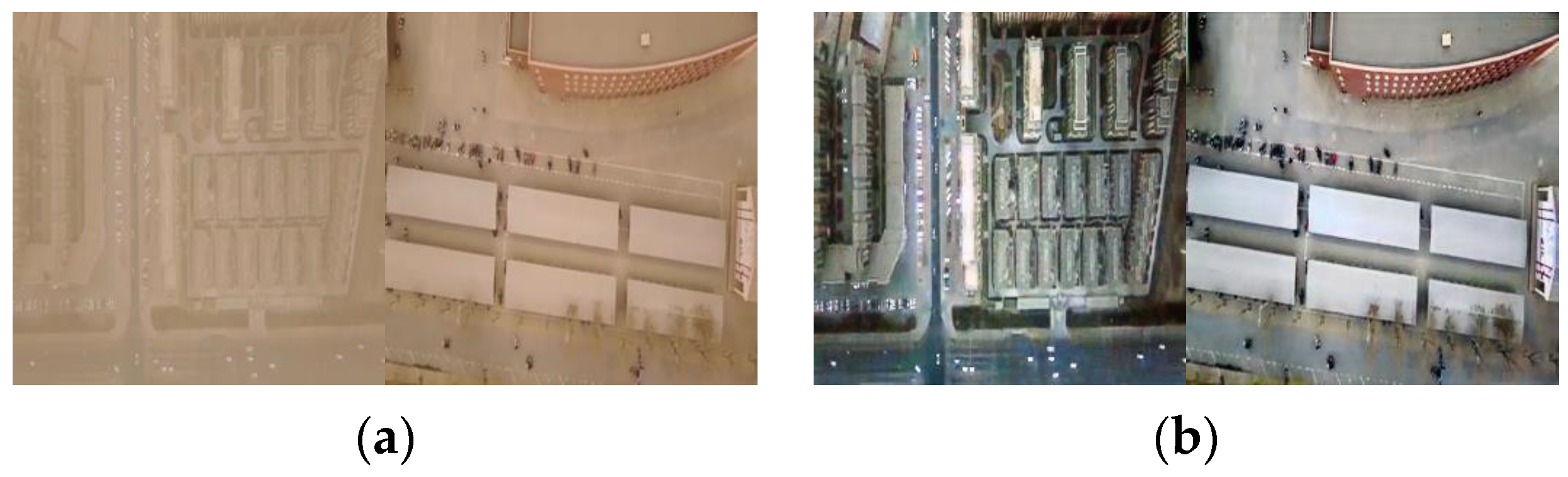
Figure 1.
Results of the proposed method; (a) Aerial sand-dust images; (b) Results of the proposed algorithm.
Figure 1.
Results of the proposed method; (a) Aerial sand-dust images; (b) Results of the proposed algorithm.

Figure 2.
The overall framework of D-CycleGAN; (a) The cycle of sand image–clean image–sand image; (b) The cycle of clean image–sand image–clean image.
Figure 2.
The overall framework of D-CycleGAN; (a) The cycle of sand image–clean image–sand image; (b) The cycle of clean image–sand image–clean image.


Figure 3.
The proposed generator structure. Here, C7S1-64 denotes a convolutional layer with a kernel size of 7, channel number of 64, and stride of 1.
Figure 3.
The proposed generator structure. Here, C7S1-64 denotes a convolutional layer with a kernel size of 7, channel number of 64, and stride of 1.

Figure 4.
Structure of the discriminator. Here, C4S2-64 denotes a convolutional layer with a kernel size of 4, channel number of 64, and stride of 2.
Figure 4.
Structure of the discriminator. Here, C4S2-64 denotes a convolutional layer with a kernel size of 4, channel number of 64, and stride of 2.

Figure 5.
Subjective effects of different components on image quality; (a) Sand-dust images; (b) Baseline; (c) Baseline+a; (d) Baseline+b; (e) Baseline+a+b; (f) Baseline+a+b+adv; (g) Baseline+a+b+adv+ploss.
Figure 5.
Subjective effects of different components on image quality; (a) Sand-dust images; (b) Baseline; (c) Baseline+a; (d) Baseline+b; (e) Baseline+a+b; (f) Baseline+a+b+adv; (g) Baseline+a+b+adv+ploss.

Figure 6.
Subjective effects of different loss functions; (a) Sand-dust images; (b) No color identity preservation loss; (c) No dual-scale semantic perceptual function; (d) The complete network model. Note that “中国气象网” and “新华网” here denote China Meteorological Network and Xinhua Network, respectively. They indicate the source of the image.

Figure 7.
Qualitative comparison results on test set ASI; (a) Aerial sand-dust images; (b) TF; (c) GDCP; (d) RDCP; (e) CC; (f) FSS; (g) VR; (h) RBCP; (i) SES; (j) AOP; (k) Proposed.
Figure 7.
Qualitative comparison results on test set ASI; (a) Aerial sand-dust images; (b) TF; (c) GDCP; (d) RDCP; (e) CC; (f) FSS; (g) VR; (h) RBCP; (i) SES; (j) AOP; (k) Proposed.


Figure 8.
Qualitative comparison results on test set NSI; (a) Natural scene sand-dust images; (b) TF; (c) GDCP; (d) RDCP; (e) CC; (f) FSS; (g) VR; (h) RBCP; (i) SES; (j) AOP; (k) Proposed.
Figure 8.
Qualitative comparison results on test set NSI; (a) Natural scene sand-dust images; (b) TF; (c) GDCP; (d) RDCP; (e) CC; (f) FSS; (g) VR; (h) RBCP; (i) SES; (j) AOP; (k) Proposed.

Figure 9.
Visualization results of the proposed method on haze images and underwater images; (a) Haze images and underwater images; (b) Enhancement results of the proposed method.
Figure 9.
Visualization results of the proposed method on haze images and underwater images; (a) Haze images and underwater images; (b) Enhancement results of the proposed method.

Figure 10.
Effect on object detection; (a) The effect of object detection for sand-dust images; (b) The effect of detection after processing by the proposed algorithm.
Figure 10.
Effect on object detection; (a) The effect of object detection for sand-dust images; (b) The effect of detection after processing by the proposed algorithm.

Figure 11.
The failure cases; (a) Sand-dust images; (b) Enhancement results of the proposed method.


Table 1.
Average SSEQ and BIQI scores for different components.
| SSEQ↓ | BIQI↓ | |
|---|---|---|
| Baseline | 14.58 | 21.06 |
| Baseline+a | 14.76 | 21.34 |
| Baseline+b | 14.04 | 19.89 |
| Baseline+a+b | 13.56 | 19.70 |
| Baseline+a+b+adv | 13.50 | 19.62 |
| Baseline+a+b+adv+ploss | 13.41 | 19.50 |
Table 2.
Average SSEQ and BIQI scores for the different loss functions.
| SSEQ↓ | BIQI↓ | |
|---|---|---|
| No vgg | 14.96 | 19.60 |
| No color | 16.09 | 22.04 |
| Ours | 13.41 | 19.50 |
Table 3.
Quantitative comparison of average SSEQ, BIQI, and PIQUE scores for the comparison algorithms on test set ASI.
Table 3.
Quantitative comparison of average SSEQ, BIQI, and PIQUE scores for the comparison algorithms on test set ASI.
| SSEQ↓ | BIQI↓ | PIQUE↓ | |
|---|---|---|---|
| TF | 25.24 | 22.55 | 37.94 |
| GDCP | 23.60 | 28.77 | 41.62 |
| RDCP | 15.23 | 37.11 | 37.72 |
| CC | 21.17 | 31.45 | 40.73 |
| FSS | 20.40 | 25.22 | 36.59 |
| VR | 24.56 | 31.48 | 42.38 |
| RBCP | 22.61 | 31.04 | 42.63 |
| SES | 19.83 | 24.02 | 39.02 |
| AOP | 19.85 | 31.60 | 33.94 |
| Proposed | 18.21 | 21.30 | 26.65 |
Table 4.
Quantitative comparison of average SSEQ, BIQI, and PIQUE scores for the comparison algorithms on test set NSI.
Table 4.
Quantitative comparison of average SSEQ, BIQI, and PIQUE scores for the comparison algorithms on test set NSI.
| SSEQ↓ | BIQI↓ | PIQUE↓ | |
|---|---|---|---|
| TF | 20.24 | 25.34 | 41.13 |
| GDCP | 18.00 | 26.37 | 41.79 |
| RDCP | 13.32 | 27.13 | 41.12 |
| CC | 16.72 | 27.22 | 42.25 |
| FSS | 14.87 | 25.22 | 40.45 |
| VR | 18.56 | 25.47 | 41.86 |
| RBCP | 18.05 | 24.85 | 41.16 |
| SES | 14.80 | 24.20 | 40.02 |
| AOP | 15.57 | 26.03 | 36.79 |
| Proposed | 13.41 | 19.50 | 33.28 |
Table 5.
Comparison of the average running time of different algorithms.
| Methods | Platform | Time (Seconds) |
|---|---|---|
| TF | MATLAB/CPU | 0.074 |
| GDCP | MATLAB/CPU | 0.279 |
| RDCP | MATLAB/CPU | 0.756 |
| CC | MATLAB/CPU | 0.132 |
| FSS | Python/CPU | 0.059 |
| VR | MATLAB/CPU | 0.165 |
| RBCP | MATLAB/CPU | 0.190 |
| SES | Python/CPU | 0.258 |
| AOP | MATLAB/CPU | 0.168 |
| Proposed | PyTorch/CPU | 0.424 |
| Proposed | PyTorch/GPU | 0.029 |
Disclaimer/Publisher’s Note: The statements, opinions and data contained in all publications are solely those of the individual author(s) and contributor(s) and not of MDPI and/or the editor(s). MDPI and/or the editor(s) disclaim responsibility for any injury to people or property resulting from any ideas, methods, instructions or products referred to in the content. |
© 2023 by the authors. Licensee MDPI, Basel, Switzerland. This article is an open access article distributed under the terms and conditions of the Creative Commons Attribution (CC BY) license (https://creativecommons.org/licenses/by/4.0/).
Share and Cite
MDPI and ACS Style
Gao, G.; Lai, H.; Jia, Z. Unsupervised Image Dedusting via a Cycle-Consistent Generative Adversarial Network. Remote Sens. 2023, 15, 1311. https://doi.org/10.3390/rs15051311
AMA Style
Gao G, Lai H, Jia Z. Unsupervised Image Dedusting via a Cycle-Consistent Generative Adversarial Network. Remote Sensing. 2023; 15(5):1311. https://doi.org/10.3390/rs15051311
Chicago/Turabian StyleGao, Guxue, Huicheng Lai, and Zhenhong Jia. 2023. "Unsupervised Image Dedusting via a Cycle-Consistent Generative Adversarial Network" Remote Sensing 15, no. 5: 1311. https://doi.org/10.3390/rs15051311
Note that from the first issue of 2016, this journal uses article numbers instead of page numbers. See further details here.