
A Multi-Scale Pseudo-Siamese Network with an Attention Mechanism for Classification of Hyperspectral and LiDAR Data

1
College of Oceanography and Space Informatics, China University of Petroleum (East China), Qingdao 266580, China
2
Laboratory for Marine Mineral Resources, Qingdao National Laboratory for Marine Science and Technology, Qingdao 266071, China
*
Author to whom correspondence should be addressed.
Remote Sens. 2023, 15(5), 1283; https://doi.org/10.3390/rs15051283
Submission received: 26 January 2023
/
Revised: 17 February 2023
/
Accepted: 20 February 2023
/
Published: 25 February 2023
Abstract
:For the remote sensing classification task, the ability of a single data source to identify the ground objects remains limited due to the lack of feature diversity. As the typical remote sensing data sources, hyperspectral imagery (HSI) and light detection and ranging (LiDAR) data can provide complementary spectral features and elevation information, respectively. To enhance classification ability, a multi-scale Pseudo-Siamese Network with attention mechanism (MA-PSNet) is proposed by fusing HSI and LiDAR data. In the network, two sub-branch networks are designed for extracting the features from HSI and LiDAR, respectively, and the connection is further established between these two branches. Specifically, a multi-scale feature learning module is incorporated, enabling the image features to be fully extracted at different scales. Similarly, a convolutional attention module is also embedded to highlight the saliency information of the objects, which makes the network training can be more targeted, thereby eventually improving the model performance for classification. The evaluation experiments of the proposed model are carried out on an urban dataset from Houston, USA, and a rural dataset from Trento, Italy. The overall accuracy (OA) of the model can reach 95.03% on the Houston data and 99.16% on the Trento data. The experimental results fully demonstrate that the proposed model has competitive performance compared with several state-of-the-art methods.
1. Introduction
As an indispensable earth observation technology, remote sensing can capture high-precision data, which provides an important scientific basis for urban planning, disaster assessment and environmental remediation. In recent years, with the increasing advancement of observation platforms and sensors, the captured remote sensing data products are evolving in a diversified direction. Currently, diverse sensors can acquire the features at different levels of the ground, such as hyperspectral sensors that capture the spectral features of an object, and LiDAR sensors that obtain three-dimensional information about the ground. Both data sources have been widely used in the task of ground object classification.
With the richness of waveband information and the characteristic of image-spectrum merging [1], hyperspectral images have been widely used in research fields such as feature classification [2,3,4,5,6], anomaly detection [7,8,9,10], and image segmentation [11,12,13,14,15], etc. However, utilization of spectral information alone is prone to misclassification, as the hyperspectral images do not contain the elevation information of ground objects [16] and are susceptible to the issues caused by “synonyms spectrum” and mixed pixels. As an active earth observation method, LiDAR can rapidly capture three-dimensional spatial information of the ground targets [17], which are perceived to be an effective supplement to hyperspectral observations. The fusion of the above two types of data helps to achieve the complementary advantages of both, thus improving the classification accuracy of ground objects [18].
So far, the research on fusing HSI and LiDAR data has been extensively carried out in different fields by numerous scholars. Dalponte et al. [19] classified tree species in complex forest areas by fusing HSI and LiDAR data, and the results showed that the fusion of two kinds of data could achieve the high-precision classification of tree species. Hartfield et al. [20] conducted a study on the classification of land cover types by fusing elevation information from LiDAR and spectral information from HSI, and the results showed that the classification accuracy of land cover types could be improved by fusing two kinds of data. For the classification of ground objects in urban areas, M. Khodadadzadeh et al. [21] proposed a multi-feature learning method that combined HSI and LiDAR data jointly, and the classification accuracy was significantly improved. The above studies indicate that the fusion of multi-source data can achieve complementary advantages and compensate for the limitations of a single data source, thus improving the classification accuracy of ground objects.
The fusion methods of multi-source data can be classified as pixel-level fusion, feature-level fusion, and decision-level fusion. Considering the data structure differences between HSI and LiDAR, the two data are more suitable for fusion at the feature level or decision level. Currently, feature-level fusion is mostly implemented using feature overlay and model-based processing. Based on the extended morphological attribute profiles (EAPs), Pedergnana et al. [22] extracted features from hyperspectral and LiDAR data, respectively, which were then fused using feature overlay with the original hyperspectral images. Rasti B et al. [23] first used extinction profiles (EPs) to extract spectral and elevation information from hyperspectral and LiDAR data and then performed model fusion using total variation component analysis. In the feature-level fusion process of HSI and LiDAR, simple concatenation or stacking of high-dimensional features may lead to the Hughes phenomenon [21]. To cope with this issue, principal component analysis (PCA) is often adopted in most studies to reduce the data dimension of hyperspectral images [24]. Decision-level fusion methods mainly include voting and statistical models [25]. Liao et al. [26] used SVM to classify the spectral features, spatial features, elevation features and fusion features, respectively, and then based on these four classification results, the decision-level fusion can thus be accomplished by weighted voting. Zhang et al. [27] fused the classification results of different data by combining the soft and hard decision fusion strategies. Zhong et al. [28] first used three classifiers, maximum likelihood estimation, SVM and polynomial logistic regression, to classify the features, respectively, and then fused all these different classification results at the decision level.
Although both feature-level fusion and decision-level fusion methods can achieve effective fusion of features, they both require considerable effort to design suitable feature extractors. Compared with traditional feature extraction methods, deep learning can mine high-level semantic features from data in an end-to-end manner [29,30]. On this basis, previous studies have shown that using deep learning to fuse HSI and LiDAR for classification can yield better classification results. By treating the LiDAR data as an additional spectral band of HSI, Morchhale et al. [31] directly input the augmented HSI to Convolutional Neural Networks (CNNs) for feature learning. Chen et al. [32] designed a two-branch network in which a CNN module was introduced in each branch to extract the features from HSI and LiDAR, respectively, and then a fully connected network was employed to fuse these extracted features. Li et al. [33] designed a dual-channel spatial, spectral, and multi-scale attention convolutional long short-term memory neural network to fuse the multiple features extracted from HSI and LiDAR data through a composite attentional learning mechanism combined with a three-level fusion module. Li et al. [34] fused the spatial, spectral and elevation information extracted from HSI and LiDAR, respectively, by designing a three-branch residual network. Zhang et al. [35] proposed an interleaving perception convolutional neural network IP-CNN, which reconstructed HSI and LiDAR data by a bi-directional self-encoder and fused the multi-source heterogeneous features extracted from these two kinds of data in an interleaved joint manner.
The multi-branch structure is an effective framework for multi-source data fusion based on deep learning. As a classical two-branch structured network, the Siamese Network [36] consists of two neural networks with the same structure and shared weights. Compared with conventional two-branch networks, Siamese Networks are often used to measure the similarity of pairs of samples by connecting two sub-networks together through a distance metric loss function, which allows the features extracted from different sub-networks to have a higher similarity. With the advantages of fewer parameters, faster calculation speed and strong correlation between branches, Siamese Networks have been widely used in the field of computer vision, such as object tracking, etc. However, the weight -sharing mechanism in Siamese Networks restricts to some extent that the difference between the two sub-branch networks cannot be too large. In other words, directly using the Siamese Network to fuse HSI and LiDAR cannot take into consideration the differences in the structure of HSI and LiDAR data, so it is necessary to achieve the multi-source heterogeneous data fusion by constructing some Pseudo-Siamese Network with superior performance.
As a popular method in the field of natural language processing and computer vision in recent years, the attention mechanism can achieve automatic focus on the target region based on the degree of feature saliency, weakening the impact caused by unnecessary features. Therefore, it is necessary to equip deep learning models with the attention mechanism to improve classification accuracy. Because the attention mechanism can adaptively assign different weights to each spectral channel and spatial region, characterizing their different levels of contribution to the classification task. At present, the attention mechanisms mainly include Non-local [37], channel attention mechanism [38], spatial attention mechanism [39], self-attention mechanisms [40], etc. Specifically, the channel attention mechanisms and spatial attention mechanisms are favored in the field of image processing due to their ability to focus on salience information in the channel and spatial domains, respectively, and both have a small number of parameters.
To fully integrate HSI and LiDAR, this paper proposes a multi-scale Pseudo-Siamese Network with an attention mechanism. This network consists of two sub-branch networks, which extract the features from HSI and LiDAR, respectively, thus further achieving decision-level data fusion of HSI spectral features, LiDAR elevation information, and the fused features of both. The main contributions of this study are given as follows:
- Considering that the distance loss function in the Pseudo-Siamese Network can enhance the correlation between different data sources, which is helpful to improve the fusion effect, this study applies Pseudo-Siamese Network to multi-source heterogeneous data fusion for the first time.
- To extract the multi-scale features of the two heterogeneous data, a multi-scale dilated convolution module is elaborately designed. The module consists of three convolutions with different dilated rates, which can consider local neighborhood information without significantly increasing the number of parameters.
- By introducing the convolutional block attention module (CBAM), each spectral channel and spatial region can be endowed with different weights adaptively to characterize their different contributions to the classification task. Therefore, the Pseudo-Siamese Network training can be more targeted based on the degree of feature saliency, enabling the model classification performance to be improved.
2. Methods
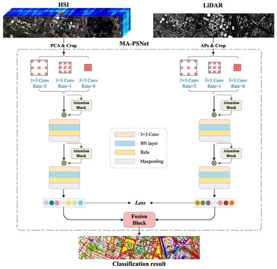
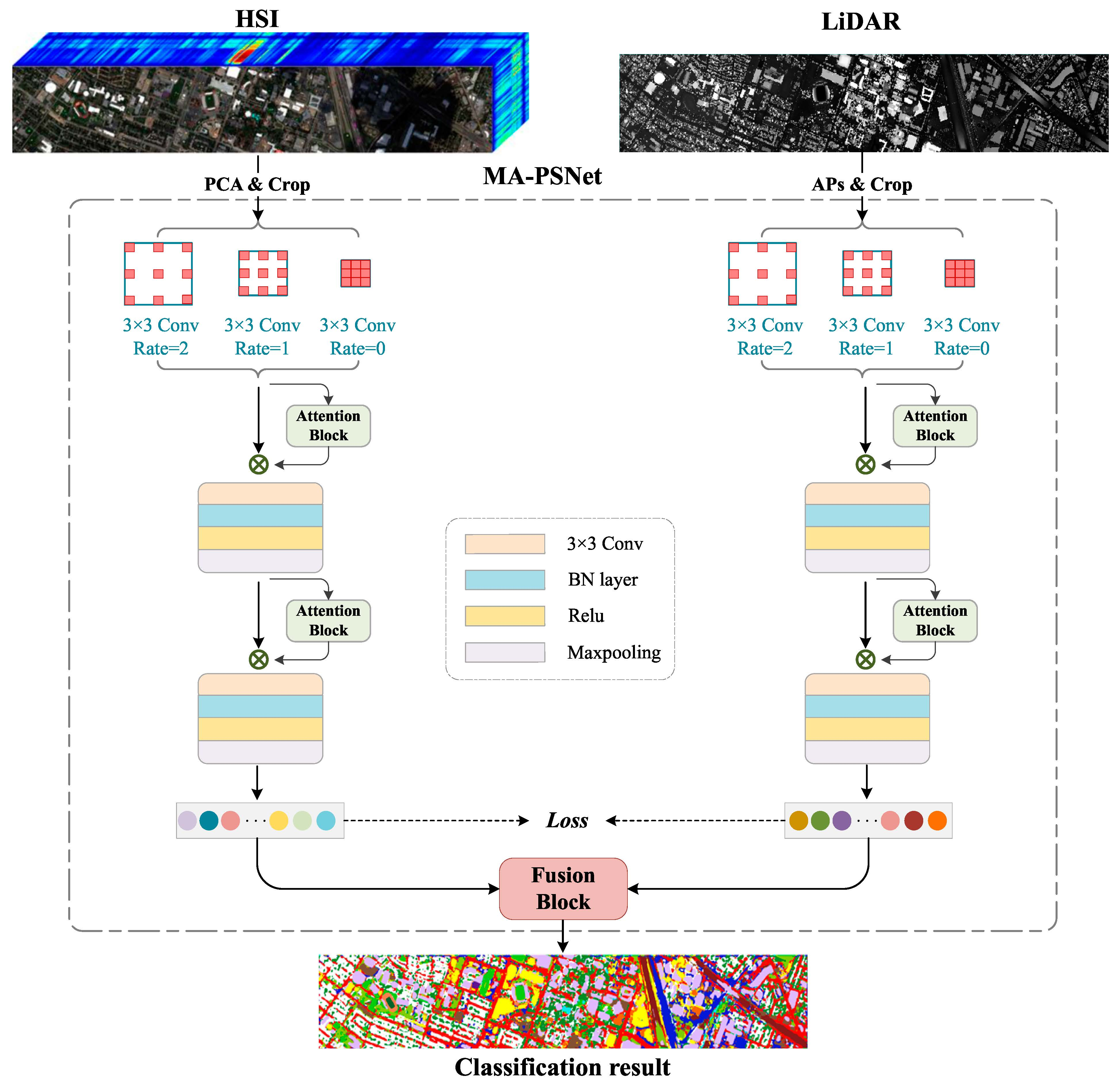
This paper proposes a multi-scale Pseudo-Siamese Network with an attention mechanism. Based on the pseudo-twin network framework, the network uses two sub-branch networks to extract the features of HSI and LiDAR respectively, which can not only consider the differences between the two data structures of HSI and LiDAR but also make the extracted two features have higher similarity, thus enhancing the connection between spectral and elevation information. In addition, to enlarge the receptive field of the image, a multi-scale cavity convolution module is introduced to obtain the feature information of the image at different scales. At the same time, a convolutional attention module is added to the network to highlight the significant information of the objects to be concerned. This module can give different weights to the features in both the channel and spatial dimensions according to their importance, thus improving the classification effect of the network model. The specific process of the method proposed in this paper is shown in Figure 1.
2.1. Multi-Scale Cavity Convolution Module
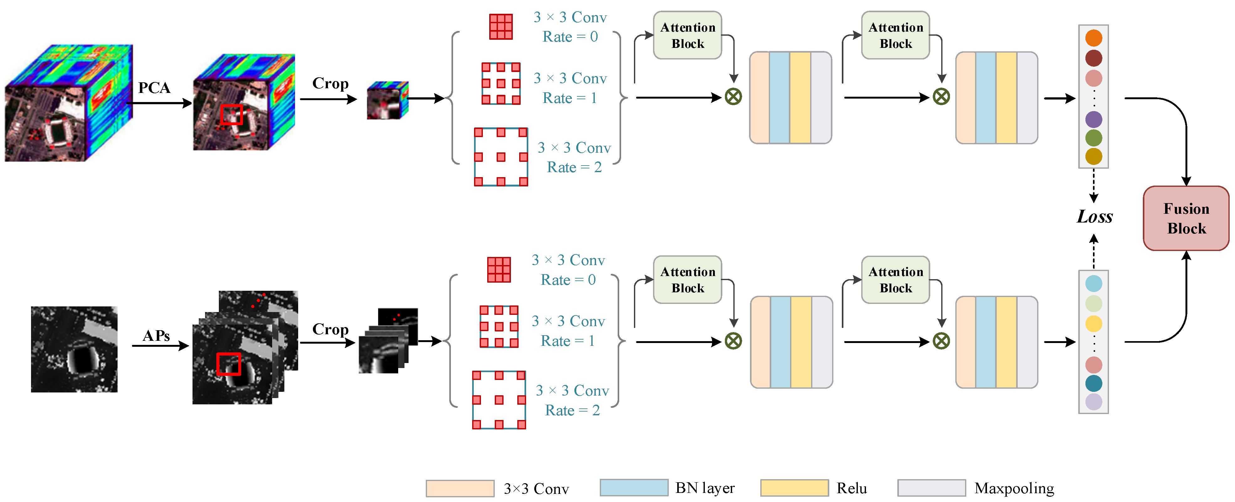
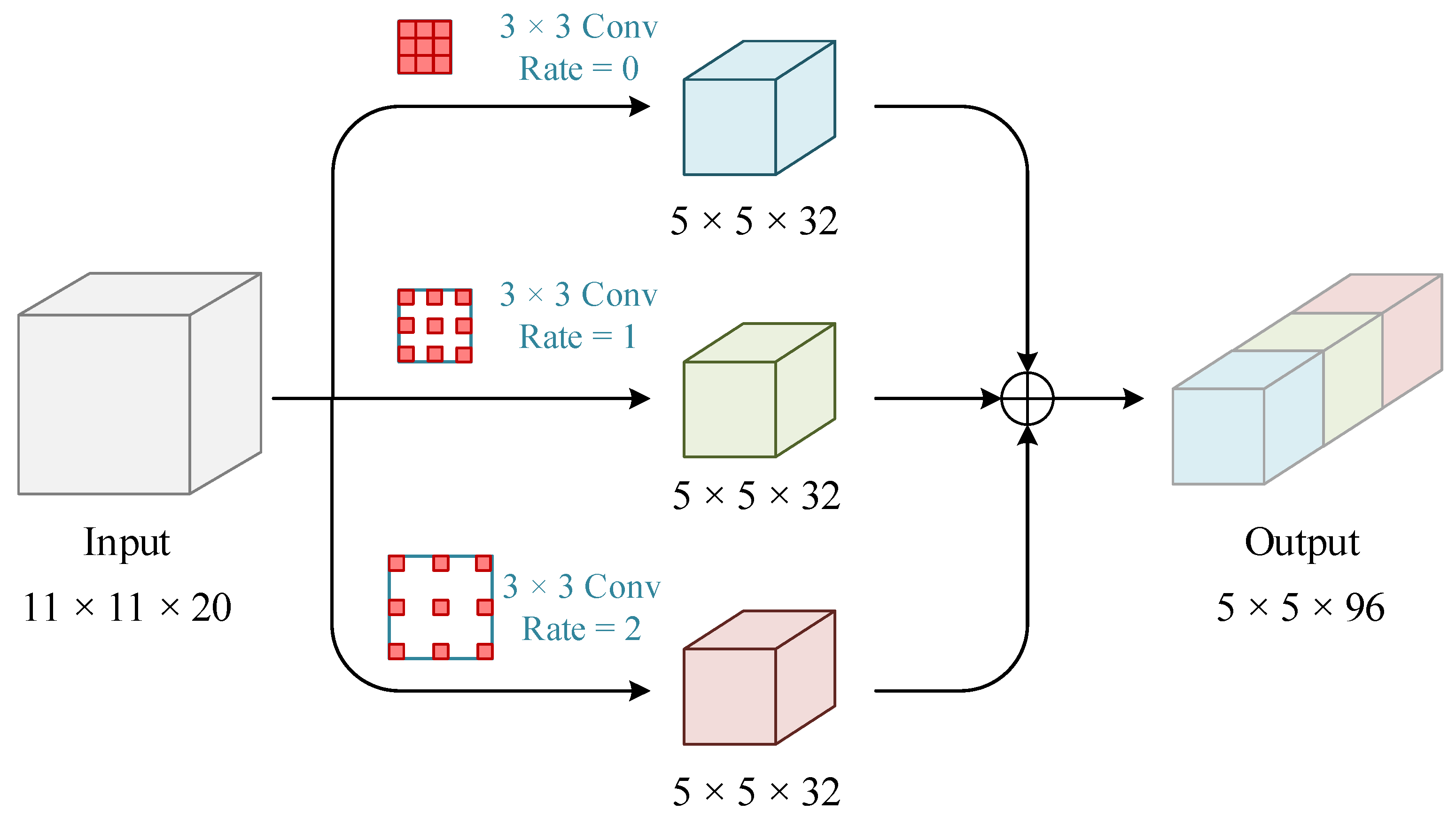
The existing feature extraction models are unable to extract the spectral and spatial features fully, the convolution scale is usually single, and the spatial context information is not sufficiently utilized during feature extraction. Thus, a multi-scale cavity convolution module is designed to capture local features at different scales in an image in light of its advantages, including increased receptive field and low computational effort. As shown in Figure 2, the module uses three convolutions with different dilated rates to extract the multi-scale feature information, and the dilated rates are set to {0, 1, 2} in this paper.
Specifically, the pre-processed HSI and LiDAR are first fed into the above multi-scale dilated convolution layers, respectively, for the multi-scale feature extraction, and the proposed features are spliced as input for the subsequent convolution layers. The introduction of dilated convolution module for multi-scale feature extraction can effectively avoid the loss of information caused by the difference in object scale.
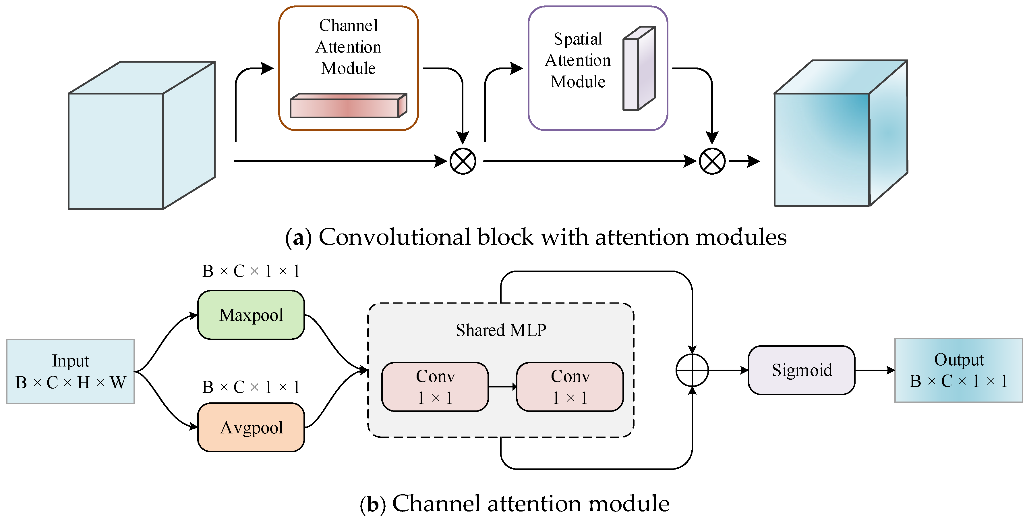
2.2. Convolutional Block Attention Module
The Convolutional Block Attention Module (CBAM) is a lightweight feedforward convolutional neural network attention module consisting of channel and spatial attention mechanisms. Its structure is shown in Figure 3. The channel attention module and spatial attention module are combined with each other in sequential order [39] and can easily be integrated into the CNN architecture (accessed after each convolutional layer) for end-to-end training. They can effectively improve the ability of the convolutional layer to extract key features and suppress unimportant features.
The channel attention module identifies the differences in the importance of different channels in the feature map.
Specifically, the Max pooling and Average pooling are firstly conducted upon each channel of the feature map , yielding two channel features and with dimensions of . Then, these two channel features are respectively fed into a shared fully connected neural network composed of a multi-layer perceptron () and a hidden layer for subsequent processing. Finally, the two processed feature maps are added together and activated by the Sigmoid function to produce the channel attention map .
The above workflow of the channel attention module can be summarized as Equation (1), where denotes the sigmoid function, and , are the weights of .
Further, the channel attention map obtained above is then multiplied with by each element to generate , which will be the input to the spatial attention module.
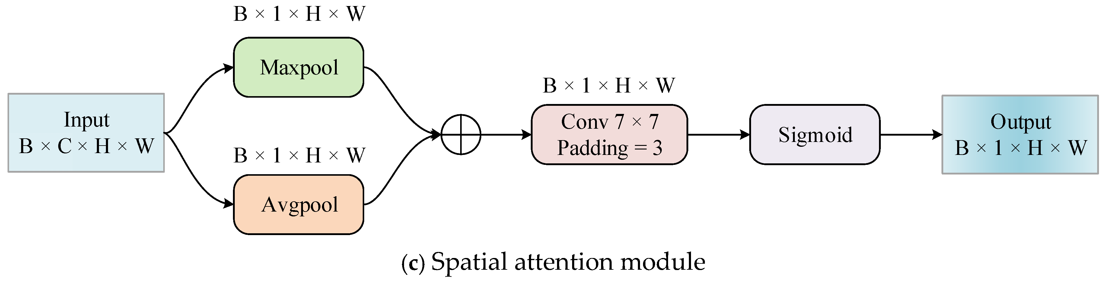
The spatial attention module is introduced to identify the difference in importance of different regions in the feature map. Its specific process is given as follows:
Firstly, the global max pooling and global average pooling are performed on each channel of to obtain the feature maps of and , respectively. Later, these two feature maps are spliced together and processed by a convolution with kernel size of . After one more step of activation by the sigmoid function, the spatial attention feature map is finally produced. The above process can be summarized as Equation (2), where and represent the activation function and convolution layer with convolution kernel, respectively.
At this point, the ultimate feature map can thus be obtained by multiplying the corresponding elements of and .
The whole CBAM process above can be equivalent to Equation (3), where the symbol denotes the element-by-element multiply operation.
2.3. Fusion Strategy
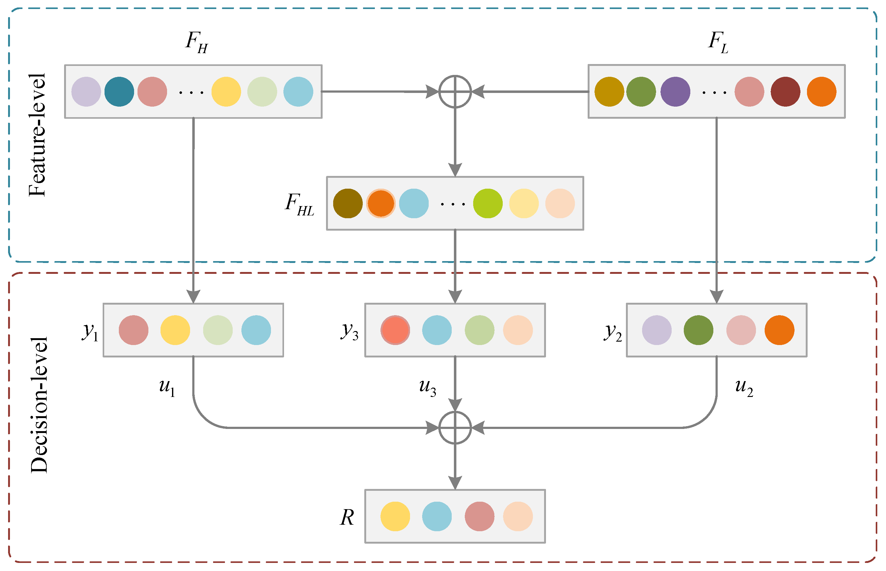
Relevant studies have confirmed that the fusion of spectral features from HSI with elevation information from LiDAR can effectively improve the ability of ground target classification [41]. Existing deep learning models typically perform feature fusion by usually stacking the extracted features together and then processing them by means of several fully connected layers to achieve the final feature fusion. However, due to a large number of parameters in the fully connected layer, the insufficient number of training samples will lead to increased difficulty in model training. To this end, this paper develops a fusion strategy based on a combination of feature-level and decision-level fusions for achieving better classification results. The logical structure of this fusion strategy is shown in Figure 4.
The feature-level fusion is to obtain a new feature by fusing features and , which are learned from HSI and LiDAR, respectively. These two features are fused by summing their corresponding pixels, as in Equation (4).
As presented in Figure 4, suppose , and are the output results corresponding to the above three features , and . Moreover, the final classification results are obtained through the decision-level fusion, which is achieved using the weighted summation, as shown in Equation (5).
where the symbol denotes the element-based product operator. , and are the weights corresponding to the three output results, respectively.
The whole fusion process above can be expressed as Equation (6):
where represents the final output of the fusion module, and denotes the decision-level fusion; , , are the three output layers, and , , are their corresponding weights.
2.4. Loss Function
By enhancing the connection between spectral information and elevation information, the ground object features expressed based on multi-source data can have higher similarity, thus contributing to improving the subsequent feature fusion effect. As shown in Figure 1, the proposed method introduces a distance loss function into feature fusion to supervise the feature learning similarity using two kinds of data.
Assuming that and are the input samples of HSI and LiDAR respectively, and , are the vectors corresponding to and in the feature space, the loss value of their similarity can thus be calculated as follows:
Assuming that are the three outputs corresponding to each sample , then their loss values can be calculated through the cross-entropy loss function as follows.
where , and is the number of training samples.
According to Equation (8) above, three loss values , and can be calculated. Thereinto, and are responsible for supervising the process of HSI and LiDAR feature learning, respectively, and is used for the process of HSI and LiDAR data fusion. The final total loss is actually a weighted combination of , , and , as expressed in Equation (9).
where , , and represent the weight parameters of , , and , respectively. In this method, , and is set to 0.01 while is set to 1.
During the implementation process, can optimize the network using the backpropagation algorithm. Moreover, , and can also be served as the regularization terms for , as such practice can widely reduce the overfitting risk in the process of network training. In the end, the test set is input into the trained network for classification prediction so as to accomplish the classification of ground objects.
3. Experiments
3.1. Datasets
The effectiveness of the proposed model in this paper was tested by the experiments on two datasets.
3.1.1. Houston 2013 Dataset
The Houston 2013 dataset consists of a hyperspectral image and a LiDAR -derived image, which were acquired on 23 June 2012 from an urban area of Houston, USA. Both data images have 349 × 1905 pixels. The HIS data was collected by the compact Airborne Spectral Imager, which recorded 144 spectral bands ranging from 380 nm to 1050 nm with a spatial resolution of 2.5 m. Figure 5 shows the pseudo-color image for HSI data, the grayscale image for LiDAR data, and the training and test data maps. There are 15 land feature types in total, and the detailed sample quantity of each type is shown in Table 1.
3.1.2. Trento Dataset
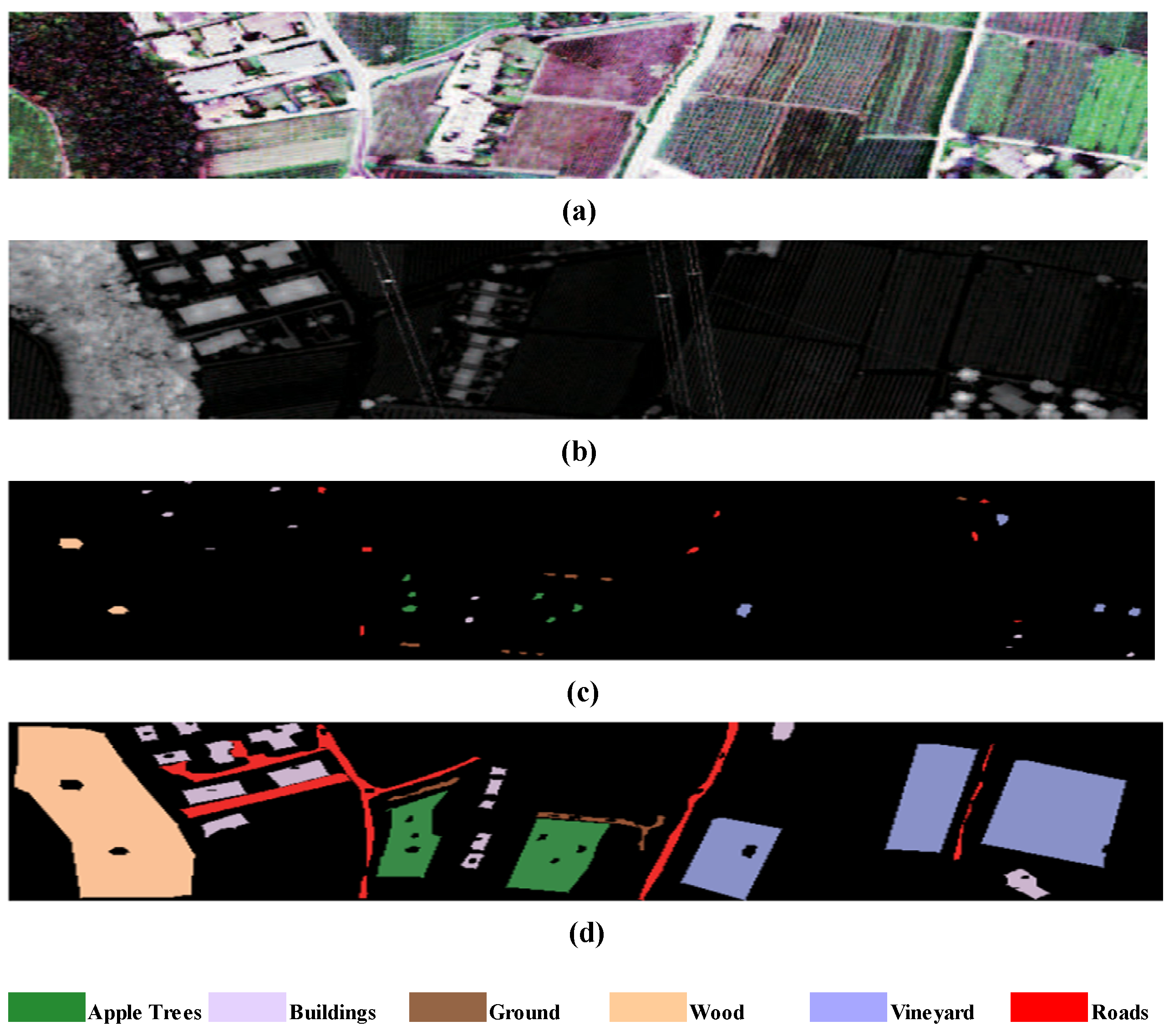
The Trento dataset was collected in a rural area south of the city of Trento, Italy. The LiDAR and HSI data were obtained by the Optech ALTM 3100EA and AISA Eagle sensors, respectively. Both data are composed of small images with a size of 600 × 166 pixels and a spatial resolution of 1 m. Specifically, the HSI ranges from 402.89 nm to 989.09 nm with a spectral resolution of 9.2 nm. Figure 6 is pseudo-color image for the hyperspectral data, a grayscale image for the LiDAR data, and the training and test data maps. Table 2 shows the number of training and test samples for different categories.
3.2. Data Pre-Processing
Due to the large number of hyperspectral image bands and the strong correlation among the bands, this paper first uses principal component analysis (PCA) to downscale the hyperspectral images and uses the top 20 extracted principal components as the data input of the hyperspectral branching network. Meanwhile, to better utilize the spatial information of LiDAR data, the morphological attribute profiles (APs) [42] were used to extend the LiDAR gray image to 21 bands, which was used as the data input of the LiDAR branch network. Similarly, to improve the model accuracy and model convergence speed, these two types of data were normalized separately using Equation (10) below.
where is the pixel value in the band and is the normalized pixel value.
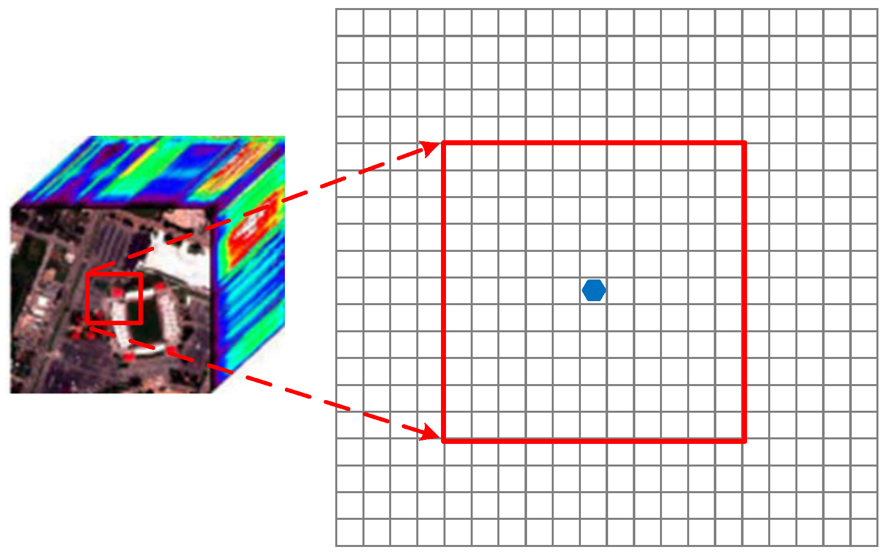
To increase model stability and reduce computational effort, HSI and LiDAR data were cropped by taking the 11 × 11 neighborhoods of each pixel as the sample to provide the spectral and spatial information, respectively, and the pixel category was used as the label, as shown in Figure 7. Then, the processed spectral sample dataset, spatial sample dataset and sample label set were divided into two parts: a training set and a test set. The specific parameters of these two sets are shown in Table 1 and Table 2.
3.3. Experimental Setup
To evaluate the performance of the proposed model, it was compared with several different models in a comprehensive manner. Specifically, only HSI or LiDAR was first used for ground feature classification by a single branch network, respectively, to highlight the advantages of feature classification based on multi-source data. Meanwhile, ablation experiments were carried out by constructing different comparison models for Houston and Trento data, respectively, to verify the effectiveness of multi-scale null convolution and convolutional attention modules.
The experiments in this study were conducted in the PyTorch framework. With its advantages of faster convergence and simpler tuning of the parameters, the Adam optimizer was adopted to optimize the parameters in the model, and its hyperparameters were set to = 0.9, = 0.999, = 10−8. The learning rate, training epochs and batch size were set to 0.001, 200, and 64, respectively. The experiments were implemented on a computer with an Intel core i7-7700K CPU 4.20 GHz processor, 16-GB RAM, and a GTX TITAN X graphic card.
The evaluation indexes for the classification results of this model include overall accuracy (), average accuracy (), accuracy per class and coefficient. refers to the overall classification accuracy, which is the ratio between the number of correctly classified pixels and the total number of pixels in the test set, refers to the average accuracy across all categories, and the coefficient is a metric used for consistency testing to measure the effectiveness of classification. The overall accuracy (), average accuracy () and coefficient are calculated as follows:
where: represents the diagonal element of the confusion matrix; denotes the sum of rows for a certain feature class; denotes the sum of columns for a feature class; is the total number of sample points evaluated, and represents the number of feature categories.
3.4. Experimental Results
In this paper, the model MA-PSNet was proposed on the basis of PSNet. To validate its effectiveness, in addition to designing two single data source models: PSNet (H) and PSNet (L), the models M-PSNet and A-PSNet, which are constructed by embedding PSNet with multi-scale cavity convolution and convolutional block attention modules, respectively, are used as the comparisons for the experiments. Table 3 and Table 4 show the detailed classification results of the six models based on Houston data and Trento data, respectively.
Firstly, the experimental results on these two datasets show that the classification performance of PSNet (H) is significantly better than that of PSNet (L), which indicates that the spectral-spatial information of HSI can provide stronger assistance for ground object identification than the elevation information of LiDAR data. Similarly, the experimental results also show that the classification accuracy of the remaining models based on both data sources is significantly higher than that of PSNet (H), which indicates that the classification performance can be significantly improved by using LiDAR data as Supplementary Information to the hyperspectral data. Secondly, it can be seen from the classification results of A-PSNet in Table 3 and Table 4 that introducing the convolutional attention module to PSNet can improve the classification performance, which is because the convolutional attention module can enhance the regions of interest of the images and suppress the useless information, making the learned features of the features more accurate and thus improving the classification ability. Meanwhile, it can be seen from the classification results of M-PSNet that adding the multi-scale feature learning module to PSNet can also improve the classification performance. This is because the multi-scale feature learning module can improve the classification accuracy by learning the scale information better and avoiding the problems of image resolution reduction and loss of feature information due to downsampling.
Finally, it is clearly observed that an improvement in the classification accuracy of PSNet when the convolutional attention module and the multi-scale feature learning module are respectively added to PSNet. Moreover, the overall accuracy of MA-PSNet is higher than that of other networks on the Houston 2013 dataset and Trento dataset. The improvement in classification accuracy can be attributed to the extraction of multi-scale features and the use of saliency information, which also confirms the effectiveness of the multi-scale feature learning module and the convolutional attention module.
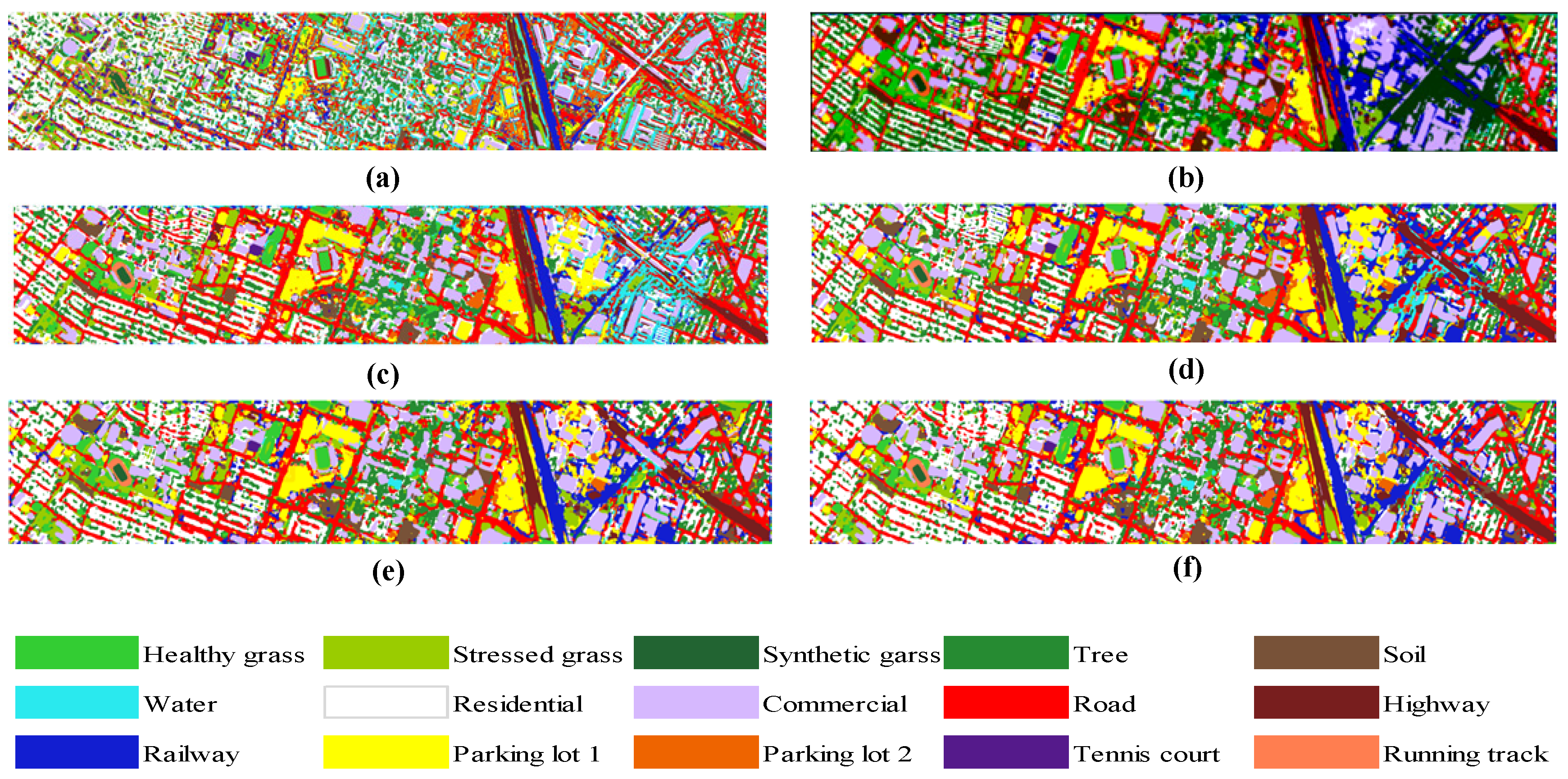
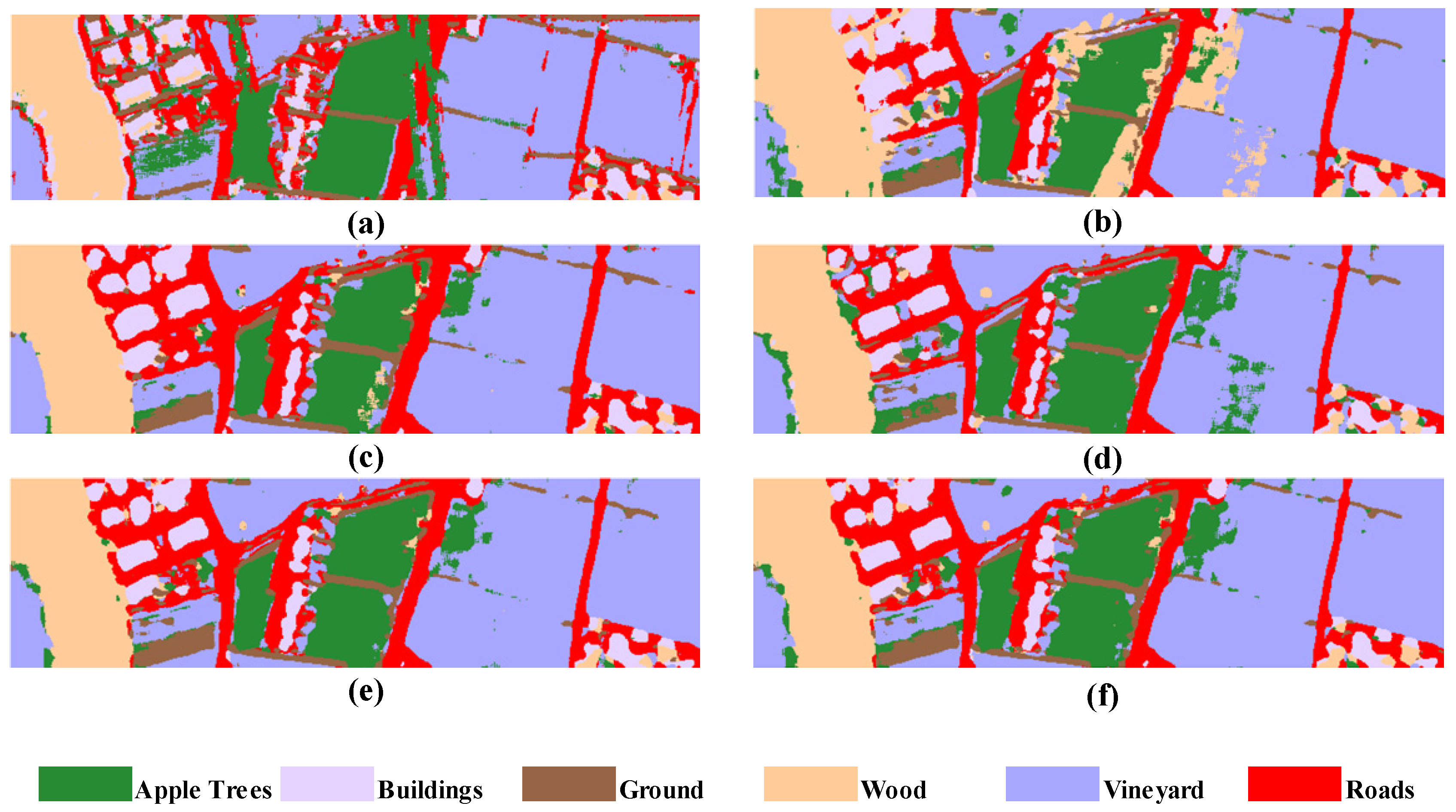
Figure 8 and Figure 9 display the classification results of Houston 2013 and Trento data sets, respectively. It is remarkable that the complex structure of the cities included in the Houston 2013 dataset poses some challenges to the classification task. Compared with the Houston dataset, the Trento dataset contains fewer types of ground objects and has a large-scale range. Thus, all models are able to obtain relatively acceptable classification results.
As seen in Figure 8a,b, the single data input is deficient in distinguishing between categories such as Highway and Residential, while the multi-source data fusion approach (Figure 8c–f) is able to produce more accurate classification results. As can be seen from Figure 8b, using only LiDAR is deficient in distinguishing between Ground and Roads categories. Although HSI (Figure 9a) is able to achieve acceptable classification accuracy, it is still slightly deficient compared to the multi-source data fusion approach (Figure 9c–f). From the above experimental results, it can be found that the classification results of the multi-source data fusion method are significantly superior to that of the classification methods based on a single data source. Moreover, the performance of PSNet can be further improved if introducing the convolutional attention module and the multi-scale feature learning module, respectively. The model with both of these two modules, MA-PSNet, has the best classification performance.
4. Discussion
4.1. Comparison with State-of-the-Art Models
To validate the superiority of the proposed model, some current state-of-the-art models are used for the comparative experiments. These comparison models include the traditional fusion classification methods: the subspace multinomial logistic regression classifier (MLRsub [21]); the total variation component analysis model (OTVCA) [23]; the sparse low-rank component analysis model (SLRCA) [43], and deep learning-based classification methods: the deep fusion method (DeepFusion) [32], the Coupled Residual Convolutional Neural Networks (CResNet) [34] and the Deep Encoder–Decoder Networks (EndNet) [44]. Given that the Houston 2013 dataset is one of the most widely used datasets in research efforts to fuse HSI and LiDAR up to now, the comparison experiments are conducted on the Houston 2013 dataset. It is worth noting that all of the above models use the same training and test sets.
The detailed comparison results of different models in terms of classification accuracy metrics , and coefficients are given in Table 5. Among the traditional methods, OTVCA achieved the highest , and coefficients, which were 92.45%, 92.68% and 0.9181, respectively. Among the deep learning models, CResNet-AUX achieved the highest , and coefficients, which were 93.57%, 93.44%, and 0.9302, respectively, while the MA-PSNet method proposed in this paper outperformed these two methods in terms of all accuracy indexes, and its model validity was verified.
4.2. Pseudo-Siamese Network
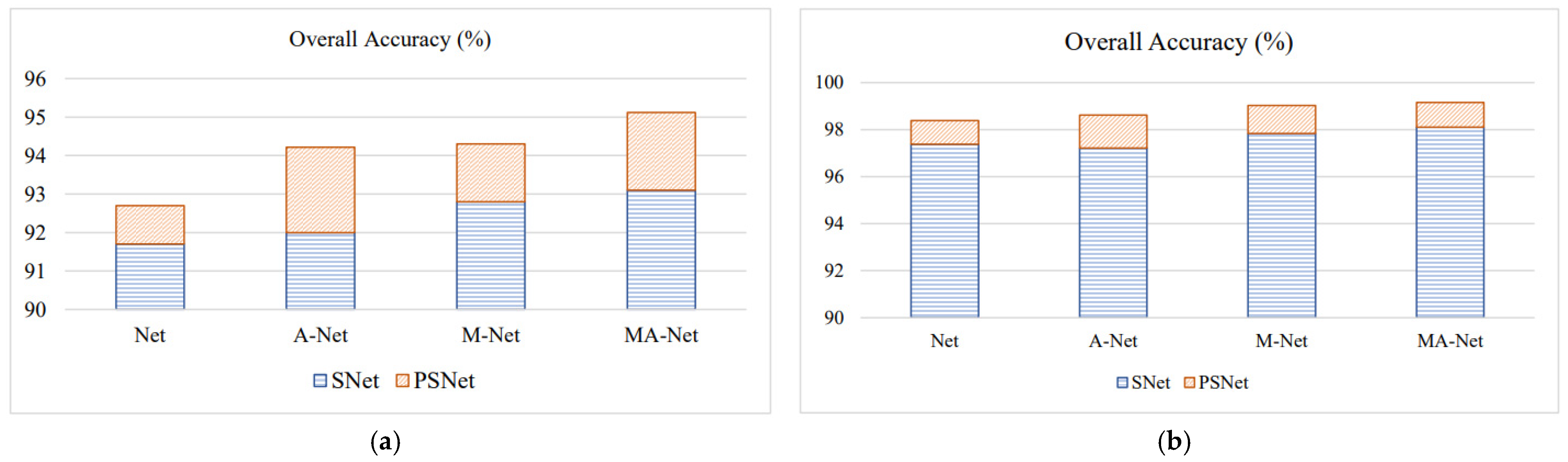
In order to highlight the superiority of the Pseudo-Siamese Network over the pseudo-twin network, the convolutional attention module and multi-scale cavity convolution are embedded into the Siamese Network (SNet) and the Pseudo-Siamese Network (PSNet), respectively, yielding A-SNet, A-PSNet, M-SNet, M-PSNet, MA-SNet, MA-PSNet as the comparison models. The experiments were conducted on the Houston and Trento datasets, respectively. Figure 10 shows the comparison results of the above network models in terms of overall classification accuracy, where the results for the Siamese network framework are shown in blue, and those for the Pseudo-Siamese Network framework are shown in orange. It is obvious from the results that the Pseudo-Siamese Network framework has better classification accuracy compared to the twin network. This may be due to the weight -sharing strategy of the convolutional layers in the Siamese Network, which reduces the number of parameters but affects the learning effect of the two network branches. However, each sub-network in the Pseudo-Siamese Network is trained independently, which can improve the learning effect of each sub-network and, thus, ultimately improve the classification accuracy.
4.3. Validation of Attribute Profiles
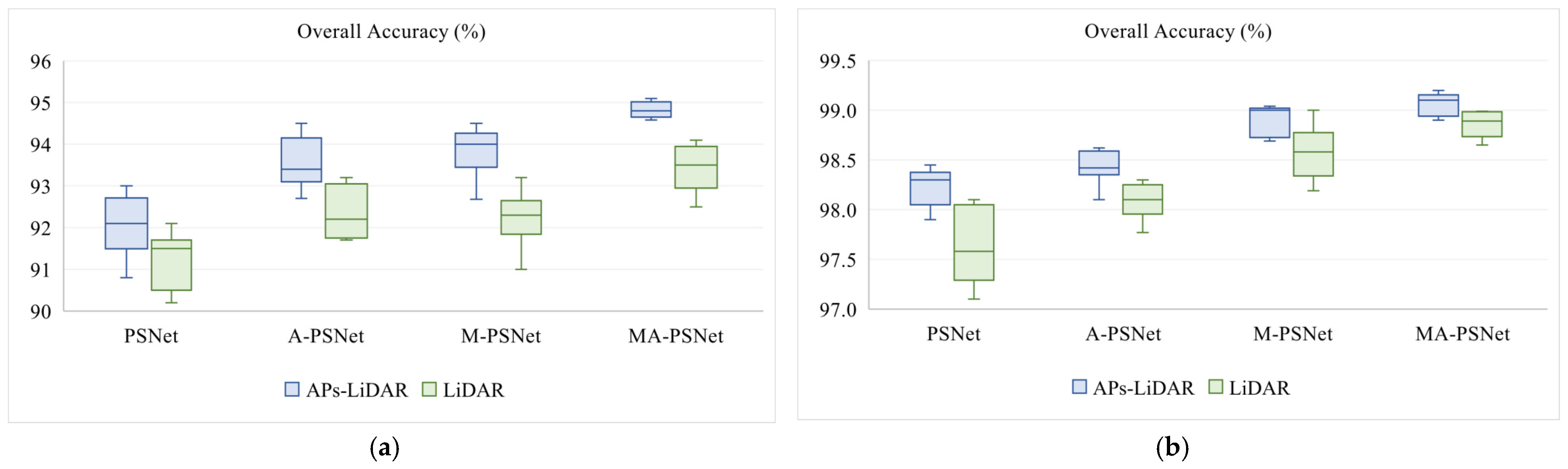
To maximize the spatial information of LiDAR data, point cloud data has been enhanced by using Aps here. Accordingly, comparative experiments are conducted on the Houston and Trento datasets to verify the effect of data enhancement. The raw LiDAR data and the LiDAR data enhanced by APs are input into the networks (PSNet, A-PSNet, M-PSNet and MA-PSNet as described in Section 3.4), respectively, and the classification performance of each method is evaluated by the overall accuracy. In Figure 11, the green box plot represents the original LiDAR data, and the blue box plot represents the LiDAR data enhanced by APs. It can be clearly seen that the experimental results based on LiDAR data enhanced by using APs have a better classification effect. This can be attributed to the fact that APs can not only extract rich structural information from LiDAR but also effectively expand the feature dimensions to achieve data enhancement, thus improving the classification performance.
4.4. Weight Parameter of the Loss Function
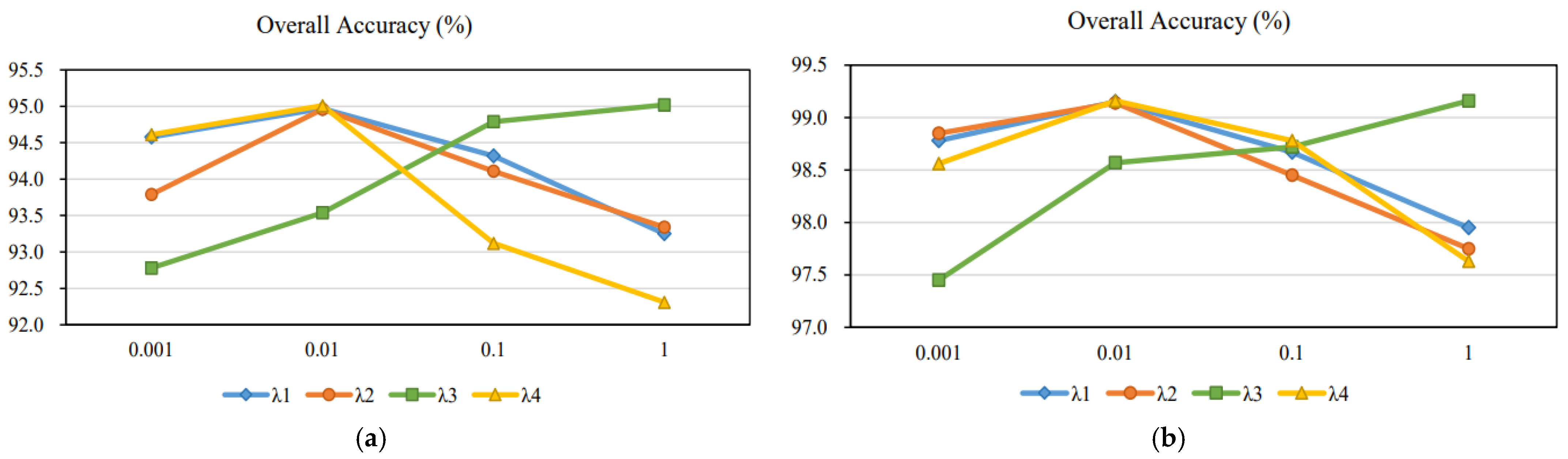
The parameter setting of the loss function can have an impact on the classification performance. There are four hyper-parameters (, , and ) in the loss function of the proposed model described in Section 2.4. To examine their impact on classification performance, the exploring experiments are conducted on Houston and Trento data sets, respectively. These experiments are carried out by firstly changing from a candidate set of {0.001, 0.01, 0.1, 1} while fixing the other parameters , , . Then, the optimal value of each hyperparameter is searched for sequentially in a similar manner. Figure 12 shows the of the corresponding classification results when the proposed MA-PSNet is set with different hyperparameters on the Huston and Trento data, respectively. The results show that the values increase and then decrease with the increase of , and . The maximum value of is obtained when these hyperparameters are set to 0.01. However, the OA value increases with the increase of . This is because the loss function term corresponding to the weight parameter plays a dominant role in constraining the fusion classification process of HSI and LiDAR data. To sum up, set , and are set as 0.01 and s set as 1.
4.5. Computation Cost
To quantitatively evaluate the computational cost of the different models, Table 6 and Table 7 show the computational time of these models on the Houston and Trento data, respectively. As can be seen from these two tables, since the PSNet (L) and PSNet (H) models only need to process single-source data, the training time is significantly shorter compared to the other fusion models. Meanwhile, it can be found that the training time of A-PSNet is approximately the same as that of PSNet. This can be interpreted that the convolutional attention module is a lightweight module; thus, embedding such a module into PSNet does not significantly increase the computational cost. In contrast, because the multi-scale feature learning module contains three convolutional layers, it makes the number of parameters and computation significantly higher, which results in a longer training time for M-PSNet and MA-PSNet. In particular, it is worth noting that once the networks have been trained, they are all tested very efficiently, with execution times essentially close to those of other existing models, and can achieve higher classification accuracy. Therefore, the additional computational cost is justified for our proposed framework.
5. Conclusions
To achieve multi-source data fusion classification, a multi-scale Pseudo-Siamese Network with an attention mechanism is proposed in this paper. The network consists of two branch networks, which implement feature extraction for HSI and LiDAR, respectively, and correlate the two sub-networks by establishing a loss function characterizing the similarity of the two data features. During the feature extraction stage, the feature information at different scales is first mined by the multi-scale feature learning module, which is then concatenated with two consecutive convolutional layers so as to ensure that the network model can extract multi-level feature information of ground objects. At the same time, the channel attention module and spatial attention module are introduced in the network to achieve the adaptive setting of weights for each channel layer and different spatial regions of the feature map, respectively, highlighting the salience information of the objects to be concerned. So that the network model can carry out more purposeful learning and training, thus improving the ultimate classification performance of the network. During the feature fusion stage, a combination of feature-level fusion and decision-level fusion is adopted, which can not only compress the information but also eliminate the errors caused by a single classifier so as to realize the full fusion of multi-source data and finally improve the accuracy and reliability of land cover classification. Finally, the validity of the proposed model was assessed on two multi-source datasets (i.e., Houston 2013, Trento datasets) by using competitive classification experiments. Meanwhile, the proposed method is compared with several state-of-the-art models such as MLRsub, OTVCA, SLRCA, DeepFusion, CResNet-AUX and EndNet. The experimental results show that the proposed method can effectively fuse multi-source data for feature classification and perform the best in the accuracy indexes of , and coefficient, respectively. Considering the variability in the effects of different data fusion procedures on the classification results, it is necessary to explore a more effective multi-level data fusion model in follow-up studies.
Supplementary Materials
The following supporting information can be downloaded at: https://www.mdpi.com/article/10.3390/rs15051283/s1. Huston_class; Trento_class.
Author Contributions
Conceptualization, methodology, D.S., J.G. and B.W.; software, J.G.; validation, writing—original draft preparation, D.S., J.G. and B.W.; writing—review and editing, D.S., J.G., B.W. and M.W.; visualization, J.G. and M.W.; funding acquisition, D.S. and B.W. All authors have read and agreed to the published version of the manuscript.
Funding
This work was supported by the Natural Science Foundation of Shandong Province under Grant ZR2022MD015, the Key Program of Joint Fund of the National Natural Science Foundation of China and Shandong Province under Grant U22A20586, the National Natural Science Foundation of China under Grant 41701513, 61371189 and 41772350, and the Key Research and Development Program of Shandong Province under Grant 2019GGX101033.
Data Availability Statement
Houston dataset were introduced for the 2013 IEEE GRSS Data Fusion contest. Data set links comes from http://hyperspectral.ee.uh.edu.
Acknowledgments
The authors would like to thank L. Bruzzone of the University of Trento for providing the Trento dataset. The same appreciation goes to the National Center for Airborne Laser Mapping (NCALM) at the University of Houston for providing the Houston dataset and the IEEE GRSS Image Analysis and Data Fusion Technical Committee for distributing the Houston dataset.
Conflicts of Interest
There is no conflict of interest among the authors of this paper.
Abbreviations
| AA | average accuracy |
| APs | attribute morphological profiles |
| A-PSNet | Pseudo-Siamese Network with Attention Mechanism |
| BN | batch normalization |
| CBAM | convolutional block attention module |
| CNN | convolutional neural network |
| EAPs | extended morphological attribute profiles |
| EPs | extinction profiles |
| HSI | hyperspectral imagery |
| LiDAR | Light Detection and Ranging |
| MA-PSNet | multiscale Pseudo-Siamese Network with attention mechanism |
| M-PSNet | multiscale Pseudo-Siamese Network |
| OA | overall accuracy |
| PCA | principal component analysis |
| PSNet | Pseudo-Siamese Network |
| ReLU | rectified linear unit |
| SNet | Siamese Network |
| SVM | Support Vector Machine |
References
- Gu, Y.F.; Wang, Q.W. Discriminative Graph-Based Fusion of HSI and LiDAR Data for Urban Area Classification. IEEE Geosci. Remote Sens. Lett. 2017, 14, 906–910. [Google Scholar] [CrossRef]
- Liu, B.; Yu, A.Z.; Yu, X.C.; Wang, R.R.; Gao, K.L.; Guo, W.Y. Deep Multiview Learning for Hyperspectral Image Classification. IEEE Trans. Geosci. Remote Sens. 2021, 59, 7758–7772. [Google Scholar] [CrossRef]
- Xu, Y.; Du, Q.; Li, W.; Younan, N.H. Efficient Probabilistic Collaborative Representation-Based Classifier for Hyperspectral Image Classification. IEEE Geosci. Remote Sens. Lett. 2019, 16, 1746–1750. [Google Scholar] [CrossRef]
- Peng, J.T.; Du, Q. Robust Joint Sparse Representation Based on Maximum Correntropy Criterion for Hyperspectral Image Classification. IEEE Trans. Geosci. Remote Sens. 2017, 55, 7152–7164. [Google Scholar] [CrossRef]
- Zhou, C.L.; Tu, B.; Ren, Q.; Chen, S.Y. Spatial Peak-Aware Collaborative Representation for Hyperspectral Imagery Classification. IEEE Geosci. Remote Sens. Lett. 2022, 19, 1–5. [Google Scholar] [CrossRef]
- Huang, B.X.; Ge, L.Y.; Chen, G.; Radenkovic, M.; Wang, X.P.; Duan, J.M.; Pan, Z.K. Nonlocal graph theory based transductive learning for hyperspectral image classification. Pattern Recognit. 2021, 116, 107967. [Google Scholar] [CrossRef]
- Song, S.Z.; Zhou, H.X.; Yang, Y.X.; Song, J.L.Q. Hyperspectral Anomaly Detection via Convolutional Neural Network and Low Rank with Density-Based Clustering. IEEE J. Sel. Top. Appl. Earth Obs. Remote Sens. 2019, 12, 3637–3649. [Google Scholar] [CrossRef]
- Wang, Q.; Yuan, Z.; Du, Q.; Li, X. GETNET: A General End-to-End 2-D CNN Framework for Hyperspectral Image Change Detection. IEEE Trans. Geosci. Remote Sens. 2018, 57, 3–13. [Google Scholar] [CrossRef] [Green Version]
- Tao, R.; Zhao, X.; Li, W.; Li, H.C.; Du, Q. Hyperspectral Anomaly Detection by Fractional Fourier Entropy. IEEE J. Sel. Top. Appl. Earth Obs. Remote Sens. 2019, 12, 4920–4929. [Google Scholar] [CrossRef]
- Tu, B.; Yang, X.C.; Zhou, C.L.; He, D.B.; Plaza, A. Hyperspectral Anomaly Detection Using Dual Window Density. IEEE Trans. Geosci. Remote Sens. 2020, 58, 8503–8517. [Google Scholar] [CrossRef]
- Fu, P.; Sun, X.; Sun, Q.S. Hyperspectral Image Segmentation via Frequency-Based Similarity for Mixed Noise Estimation. Remote Sens. 2017, 9, 1237. [Google Scholar] [CrossRef] [Green Version]
- Saranathan, A.M.; Parente, M. Uniformity-Based Superpixel Segmentation of Hyperspectral Images. IEEE Trans. Geosci. Remote Sens. 2016, 54, 1419–1430. [Google Scholar] [CrossRef]
- Zhang, X.R.; Zhang, J.Y.; Li, C.; Cheng, C.; Jiao, L.C.; Zhou, H.Y. Hybrid Unmixing Based on Adaptive Region Segmentation for Hyperspectral Imagery. IEEE Trans. Geosci. Remote Sens. 2018, 56, 3861–3875. [Google Scholar] [CrossRef] [Green Version]
- Leng, Q.M.; Yang, H.O.; Jiang, J.J.; Tian, Q. Adaptive MultiScale Segmentations for Hyperspectral Image Classification. IEEE Trans. Geosci. Remote Sens. 2020, 58, 5847–5860. [Google Scholar] [CrossRef]
- Huang, B.X.; Pan, Z.K.; Yang, H.; Bai, L. Variational level set method for image segmentation with simplex constraint of landmarks. Signal Process. Image Commun. 2020, 82, 115745. [Google Scholar] [CrossRef]
- Sankey, T.T.; McVay, J.; Swetnam, T.L.; McClaran, M.P.; Heilman, P.; Nichols, M. UAV hyperspectral and lidar data and their fusion for arid and semi-arid land vegetation monitoring. Remote Sens. Ecol. Conserv. 2018, 4, 20–33. [Google Scholar] [CrossRef]
- Ghamisi, P.; Rasti, B.; Yokoya, N.; Wang, Q.M.; Hofle, B.; Bruzzone, L.; Bovolo, F.; Chi, M.M.; Anders, K.; Gloaguen, R.; et al. Multisource and Multitemporal Data Fusion in Remote Sensing A comprehensive review of the state of the art. IEEE Geosci. Remote Sens. Mag. 2019, 7, 6–39. [Google Scholar] [CrossRef] [Green Version]
- Debes, C.; Merentitis, A.; Heremans, R.; Hahn, J.; Frangiadakis, N.; van Kasteren, T.; Liao, W.Z.; Bellens, R.; Pizurica, A.; Gautama, S.; et al. Hyperspectral and LiDAR Data Fusion: Outcome of the 2013 GRSS Data Fusion Contest. IEEE J. Sel. Top. Appl. Earth Obs. Remote Sens. 2014, 7, 2405–2418. [Google Scholar] [CrossRef]
- Dalponte, M.; Bruzzone, L.; Gianelle, D. Fusion of hyperspectral and LIDAR remote sensing data for classification of complex forest areas. IEEE Trans. Geosci. Remote Sens. 2008, 46, 1416–1427. [Google Scholar] [CrossRef] [Green Version]
- Hartfield, K.A.; Landau, K.I.; van Leeuwen, W.J.D. Fusion of High Resolution Aerial Multispectral and LiDAR Data: Land Cover in the Context of Urban Mosquito Habitat. Remote Sens. 2011, 3, 2364–2383. [Google Scholar] [CrossRef] [Green Version]
- Khodadadzadeh, M.; Li, J.; Prasad, S.; Plaza, A. Fusion of Hyperspectral and LiDAR Remote Sensing Data Using Multiple Feature Learning. IEEE J. Sel. Top. Appl. Earth Obs. Remote Sens. 2015, 8, 2971–2983. [Google Scholar] [CrossRef]
- Pedergnana, M.; Marpu, P.R.; Mura, M.D.; Benediktsson, J.A.; Bruzzone, L. Classification of Remote Sensing Optical and LiDAR Data Using Extended Attribute Profiles. IEEE J. Sel. Top. Signal Process. 2012, 6, 856–865. [Google Scholar] [CrossRef]
- Rasti, B.; Ghamisi, P.; Gloaguen, R. Hyperspectral and LiDAR Fusion Using Extinction Profiles and Total Variation Component Analysis. IEEE Trans. Geosci. Remote Sens. 2017, 55, 3997–4007. [Google Scholar] [CrossRef]
- Zare, A.; Ozdemir, A.; Iwen, M.A.; Aviyente, S. Extension of PCA to Higher Order Data Structures: An Introduction to Tensors, Tensor Decompositions, and Tensor PCA. Proc. IEEE 2018, 106, 1341–1358. [Google Scholar] [CrossRef] [Green Version]
- Zeng, Y.; Zhang, J.X.; Niu, R.C. Research Status and Development Trend of Remote sensing in China using Bibliometric Analysis. In Proceedings of the International Workshop on Image and Data Fusion (IWIDF), Kona, HI, USA, 21–23 July 2015; pp. 203–208. [Google Scholar]
- Liao, W.Z.; Bellens, R.; Pizurica, A.; Gautama, S.; Philips, W.; IEEE. Combining Feature Fusion and Decision Fusion for Classification of Hyperspectral and Lidar Data. In Proceedings of the IEEE Joint International Geoscience and Remote Sensing Symposium (IGARSS) / 35th Canadian Symposium on Remote Sensing, Quebec City, QC, Canada, 13–18 July 2014; pp. 1241–1244. [Google Scholar]
- Zhang, Y.H.; Yang, H.L.; Prasad, S.; Pasolli, E.; Jung, J.H.; Crawford, M. Ensemble Multiple Kernel Active Learning For Classification of Multisource Remote Sensing Data. IEEE J. Sel. Top. Appl. Earth Obs. Remote Sens. 2015, 8, 845–858. [Google Scholar] [CrossRef]
- Yanfei, Z.; Qiong, C.; Ji, Z.; Ailong, M.; Bei, Z.; Liangpei, Z. Optimal Decision Fusion for Urban Land-Use/Land-Cover Classification Based on Adaptive Differential Evolution Using Hyperspectral and LiDAR Data. Remote Sens. 2017, 9, 868. [Google Scholar]
- Hang, R.L.; Liu, Q.S.; Hong, D.F.; Ghamisi, P. Cascaded Recurrent Neural Networks for Hyperspectral Image Classification. IEEE Trans. Geosci. Remote Sens. 2019, 57, 5384–5394. [Google Scholar] [CrossRef] [Green Version]
- Zhu, X.X.; Tuia, D.; Mou, L.; Xia, G.S.; Zhang, L.; Xu, F.; Fraundorfer, F. Deep Learning in Remote Sensing: A Comprehensive Review and List of Resources. IEEE Geosci. Remote Sens. Mag. 2018, 5, 8–36. [Google Scholar] [CrossRef] [Green Version]
- Morchhale, S.; Pauca, V.P.; Plemmons, R.J.; Torgersen, T.C.; IEEE. Classification of pixel-level fused hyperspectral and lidar data using deep convolutional neural networks. In Proceedings of the 8th Workshop on Hyperspectral Image and Signal Processing—Evolution in Remote Sensing (WHISPERS), Los Angeles, CA, USA, 21–24 August 2016. [Google Scholar]
- Chen, Y.S.; Li, C.Y.; Ghamisi, P.; Jia, X.P.; Gu, Y.F. Deep Fusion of Remote Sensing Data for Accurate Classification. IEEE Geosci. Remote Sens. Lett. 2017, 14, 1253–1257. [Google Scholar] [CrossRef]
- Li, H.C.; Hu, W.S.; Li, W.; Li, J.; Du, Q.; Plaza, A. A(3)CLNN: Spatial, Spectral and Multiscale Attention ConvLSTM Neural Network for Multisource Remote Sensing Data Classification. IEEE Trans. Neural Netw. Learn. Syst. 2022, 33, 747–761. [Google Scholar] [CrossRef]
- Li, H.; Ghamisi, P.; Rasti, B.; Wu, Z.Y.; Shapiro, A.; Schultz, M.; Zipf, A. A Multi-Sensor Fusion Framework Based on Coupled Residual Convolutional Neural Networks. Remote Sens. 2020, 12, 2067. [Google Scholar] [CrossRef]
- Zhang, M.M.; Li, W.; Tao, R.; Li, H.C.; Du, Q. Information Fusion for Classification of Hyperspectral and LiDAR Data Using IP-CNN. IEEE Trans. Geosci. Remote Sens. 2022, 60, 1–12. [Google Scholar] [CrossRef]
- Zagoruyko, S.; Komodakis, N.; IEEE. Learning to Compare Image Patches via Convolutional Neural Networks. In Proceedings of the IEEE Conference on Computer Vision and Pattern Recognition (CVPR), Boston, MA, USA, 7–12 June 2015; pp. 4353–4361. [Google Scholar]
- Liu, M.; Wang, Z.Y.; Ji, S.W. Non-Local Graph Neural Networks. IEEE Trans. Pattern Anal. Mach. Intell. 2022, 44, 10270–10276. [Google Scholar] [CrossRef] [PubMed]
- Hu, J.; Shen, L.; Albanie, S.; Sun, G.; Wu, E.H. Squeeze-and-Excitation Networks. IEEE Trans. Pattern Anal. Mach. Intell. 2020, 42, 2011–2023. [Google Scholar] [CrossRef] [Green Version]
- Woo, S.H.; Park, J.; Lee, J.Y.; Kweon, I.S. CBAM: Convolutional Block Attention Module. In Proceedings of the 15th European Conference on Computer Vision (ECCV), Munich, Germany, 8–14 September 2018; pp. 3–19. [Google Scholar]
- Vaswani, A.; Shazeer, N.; Parmar, N.; Uszkoreit, J.; Jones, L.; Gomez, A.N.; Kaiser, L.; Polosukhin, I. Attention Is All You Need. In Proceedings of the 31st Annual Conference on Neural Information Processing Systems (NIPS), Long Beach, CA, USA, 4–9 December 2017. [Google Scholar]
- Priem, F.; Canters, F. Synergistic Use of LiDAR and APEX Hyperspectral Data for High-Resolution Urban Land Cover Mapping. Remote Sens. 2016, 8, 787. [Google Scholar] [CrossRef] [Green Version]
- Hong, D.F.; Wu, X.; Ghamisi, P.; Chanussot, J.; Yokoya, N.; Zhu, X.X. Invariant Attribute Profiles: A Spatial-Frequency Joint Feature Extractor for Hyperspectral Image Classification. IEEE Trans. Geosci. Remote Sens. 2020, 58, 3791–3808. [Google Scholar] [CrossRef] [Green Version]
- Rasti, B.; Ghamisi, P.; Plaza, J.; Plaza, A. Fusion of Hyperspectral and LiDAR Data Using Sparse and Low-Rank Component Analysis. IEEE Trans. Geosci. Remote Sens. 2017, 55, 6354–6365. [Google Scholar] [CrossRef] [Green Version]
- Hong, D.F.; Gao, L.R.; Hang, R.L.; Zhang, B.; Chanussot, J. Deep EncoderDecoder Networks for Classification of Hyperspectral and LiDAR Data. IEEE Geosci. Remote Sens. Lett. 2022, 19, 1–5. [Google Scholar] [CrossRef]
Figure 1.
The architecture of the proposed MA-PSNet.

Figure 2.
Structure of the multi-scale dilated convolution module.

Figure 3.
Structure of the convolutional block with attention modules.


Figure 4.
Structure of fusion strategy.

Figure 5.
Houston 2013: (a) Pseudo-color image for HSI data. (b) Grayscale image for the LiDAR data, (c) Training data map. (d) Testing data map.
Figure 5.
Houston 2013: (a) Pseudo-color image for HSI data. (b) Grayscale image for the LiDAR data, (c) Training data map. (d) Testing data map.

Figure 6.
Trento: (a) The LiDAR-derived DSM image. (b) Grayscale image for the LiDAR data. (c) Training data map. (d) Testing data map.
Figure 6.
Trento: (a) The LiDAR-derived DSM image. (b) Grayscale image for the LiDAR data. (c) Training data map. (d) Testing data map.

Figure 7.
Schematic diagram of selecting the neighborhood pixels.

Figure 8.
The Houston 2013 dataset: Classifications generated from different features and models. (a) PSNet (L), (b) PSNet (H), (c) PSNet, (d) A-PSNet, (e) M-PSNnet and (f) MA-PSNet.
Figure 8.
The Houston 2013 dataset: Classifications generated from different features and models. (a) PSNet (L), (b) PSNet (H), (c) PSNet, (d) A-PSNet, (e) M-PSNnet and (f) MA-PSNet.

Figure 9.
The Trento dataset: Classifications generated from different features and models. (a) PSNet (L), (b) PSNet (H), (c) PSNet, (d) A-PSNet, (e) M-PSNet and (f) MA-PSNet.
Figure 9.
The Trento dataset: Classifications generated from different features and models. (a) PSNet (L), (b) PSNet (H), (c) PSNet, (d) A-PSNet, (e) M-PSNet and (f) MA-PSNet.

Figure 10.
Comparison of classification accuracy between two datasets using Siamese Network and Pseudo-Siamese Network (a) Houston dataset. (b) Trento dataset.
Figure 10.
Comparison of classification accuracy between two datasets using Siamese Network and Pseudo-Siamese Network (a) Houston dataset. (b) Trento dataset.

Figure 11.
Comparison of classification accuracy before and after adopting the Aps on two datasets (a) Houston dataset. (b) Trento dataset.
Figure 11.
Comparison of classification accuracy before and after adopting the Aps on two datasets (a) Houston dataset. (b) Trento dataset.

Figure 12.
Effect of weight parameters on the classification performance of MA-PSNet. (a) Houston dataset. (b) Trento dataset.
Figure 12.
Effect of weight parameters on the classification performance of MA-PSNet. (a) Houston dataset. (b) Trento dataset.


Table 1.
Sample distribution of the Houston 2013 dataset.
| Class No. | Class Name | Training | Test |
|---|---|---|---|
| 1 | Healthy grass | 198 | 1053 |
| 2 | Stressed grass | 190 | 1064 |
| 3 | Synthetic grass | 192 | 505 |
| 4 | Tree | 188 | 1056 |
| 5 | Soil | 186 | 1056 |
| 6 | Water | 182 | 143 |
| 7 | Residential | 196 | 1072 |
| 8 | Commercial | 191 | 1053 |
| 9 | Road | 193 | 1059 |
| 10 | Highway | 191 | 1036 |
| 11 | Railway | 181 | 1054 |
| 12 | Parking lot 1 | 192 | 1041 |
| 13 | Parking lot 2 | 184 | 285 |
| 14 | Tennis court | 181 | 247 |
| 15 | Running track | 187 | 473 |
| - | Total | 2832 | 12,197 |
Table 2.
Sample distribution of Trento dataset.
| Class No. | Class Name | Training | Test |
|---|---|---|---|
| 1 | Apple trees | 129 | 3905 |
| 2 | Buildings | 125 | 2778 |
| 3 | Ground | 105 | 374 |
| 4 | Wood | 154 | 8969 |
| 5 | Vineyard | 184 | 10,317 |
| 6 | Roads | 122 | 3252 |
| - | Total | 819 | 29,595 |
Table 3.
Houston 2013: Classification accuracies for per class, , (in %), coefficient (is of no unit).
Table 3.
Houston 2013: Classification accuracies for per class, , (in %), coefficient (is of no unit).
| Category | PSNet (L) | PSNet (H) | PSNet | A-PSNet | M-PSNet | MA-PSNet |
|---|---|---|---|---|---|---|
| 1 | 63.15 | 82.91 | 82.81 | 82.90 | 88.89 | 89.17 |
| 2 | 22.56 | 85.15 | 84.40 | 96.52 | 95.30 | 95.58 |
| 3 | 41.98 | 94.26 | 95.84 | 96.04 | 95.04 | 92.47 |
| 4 | 86.96 | 92.14 | 99.90 | 99.24 | 98.77 | 98.48 |
| 5 | 30.02 | 100 | 99.81 | 100 | 99.43 | 99.81 |
| 6 | 34.27 | 96.50 | 92.30 | 94.41 | 90.21 | 95.24 |
| 7 | 74.81 | 85.73 | 92.53 | 91.14 | 94.22 | 94.77 |
| 8 | 85.19 | 94.49 | 97.05 | 94.68 | 96.96 | 97.43 |
| 9 | 50.24 | 87.91 | 90.27 | 91.60 | 92.63 | 93.20 |
| 10 | 51.83 | 62.93 | 87.74 | 94.59 | 84.27 | 89.77 |
| 11 | 87.95 | 97.63 | 93.73 | 94.12 | 93.93 | 94.12 |
| 12 | 34.10 | 97.12 | 95.10 | 95.49 | 99.33 | 99.14 |
| 13 | 69.82 | 91.93 | 85.61 | 92.98 | 87.72 | 89.96 |
| 14 | 69.23 | 90.59 | 100 | 89.47 | 91.09 | 91.47 |
| 15 | 42.92 | 99.36 | 98.52 | 99.79 | 98.52 | 100 |
| 57.59 | 89.48 | 92.72 | 94.22 | 94.30 | 95.03 | |
| 56.33 | 90.57 | 93.04 | 94.19 | 93.75 | 94.70 | |
| 0.5554 | 0.8868 | 0.9066 | 0.9376 | 0.9384 | 0.9463 |
The bold refers to the best , , and performance.
Table 4.
Trento: Classification accuracies for per class, , (in %), coefficient (is of no unit).
| Category | PSNet (L) | PSNet (H) | PSNet | A-PSNet | M-PSNet | MA-PSNet |
|---|---|---|---|---|---|---|
| 1 | 99.92 | 99.59 | 97.75 | 99.62 | 99.46 | 99.36 |
| 2 | 91.00 | 93.23 | 98.99 | 97.91 | 98.60 | 98.81 |
| 3 | 61.76 | 90.64 | 93.05 | 82.62 | 94.65 | 94.65 |
| 4 | 97.32 | 99.44 | 100 | 99.41 | 99.96 | 99.91 |
| 5 | 92.36 | 99.88 | 100 | 99.97 | 99.96 | 99.91 |
| 6 | 53.83 | 82.83 | 89.56 | 93.05 | 93.51 | 95.02 |
| 90.36 | 97.19 | 98.38 | 98.62 | 99.03 | 99.16 | |
| 82.70 | 94.27 | 96.56 | 95.43 | 97.69 | 97.94 | |
| 0.8744 | 0.962 | 0.9784 | 0.9816 | 0.9871 | 0.9888 |
The bold refers to the best , , and performance.
Table 5.
Comparisons of classification accuracy with different models on Houston 2013 dataset.
| Methods | Traditional Models | Deep Learning Model | Proposed | ||||
|---|---|---|---|---|---|---|---|
| MLRsub | OTVCA | SLRCA | DeepFusion | CResNet-AUX | EndNet | MA-PSNet | |
| (%) | 92.05 | 92.45 | 91.30 | 91.32 | 93.57 | 88.52 | 95.03 |
| (%) | 92.85 | 92.68 | 91.95 | 91.96 | 93.44 | 89.95 | 94.70 |
| 0.9137 | 0.9181 | 0.9056 | 0.9057 | 0.9302 | 0.8759 | 0.9463 | |
The bold refers to the best , and performance.
Table 6.
The computation time of different models on the Houston 2013 dataset.
| Houston 2013 | PSNet (L) | PSNet (H) | PSNet | A-PSNet | M-PSNet | MA-PSNet |
|---|---|---|---|---|---|---|
| Train (min) | 4.30 | 4.41 | 5.47 | 5.65 | 6.50 | 6.82 |
| Test (s) | 1.89 | 1.98 | 2.10 | 2.06 | 2.28 | 2.30 |
Table 7.
The computation time of different models on the Trento dataset.
| Houston 2013 | PSNet (L) | PSNet (H) | PSNet | A-PSNet | M-PSNet | MA-PSNet |
|---|---|---|---|---|---|---|
| Train (min) | 2.17 | 2.28 | 3.15 | 3.38 | 3.72 | 3.91 |
| Test (s) | 2.10 | 2.14 | 2.32 | 2.25 | 2.54 | 2.70 |
Disclaimer/Publisher’s Note: The statements, opinions and data contained in all publications are solely those of the individual author(s) and contributor(s) and not of MDPI and/or the editor(s). MDPI and/or the editor(s) disclaim responsibility for any injury to people or property resulting from any ideas, methods, instructions or products referred to in the content. |
© 2023 by the authors. Licensee MDPI, Basel, Switzerland. This article is an open access article distributed under the terms and conditions of the Creative Commons Attribution (CC BY) license (https://creativecommons.org/licenses/by/4.0/).
Share and Cite
MDPI and ACS Style
Song, D.; Gao, J.; Wang, B.; Wang, M. A Multi-Scale Pseudo-Siamese Network with an Attention Mechanism for Classification of Hyperspectral and LiDAR Data. Remote Sens. 2023, 15, 1283. https://doi.org/10.3390/rs15051283
AMA Style
Song D, Gao J, Wang B, Wang M. A Multi-Scale Pseudo-Siamese Network with an Attention Mechanism for Classification of Hyperspectral and LiDAR Data. Remote Sensing. 2023; 15(5):1283. https://doi.org/10.3390/rs15051283
Chicago/Turabian StyleSong, Dongmei, Jiacheng Gao, Bin Wang, and Mingyue Wang. 2023. "A Multi-Scale Pseudo-Siamese Network with an Attention Mechanism for Classification of Hyperspectral and LiDAR Data" Remote Sensing 15, no. 5: 1283. https://doi.org/10.3390/rs15051283
Note that from the first issue of 2016, this journal uses article numbers instead of page numbers. See further details here.