
An Extended Robust Chance-Constrained Power Allocation Scheme for Multiple Target Localization of Digital Array Radar in Strong Clutter Environments

Abstract
:
1. Introduction
1.1. Background and Motivation
1.2. Major Contributions
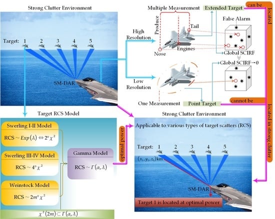
- Aiming at the characteristics of strong clutter in the current detection environment, we propose an ERCC-PA scheme to solve the power allocation problem of high-resolution SM-DAR locating multiple extended targets in strong clutter. This scheme rigorously derives the SCIRF that high-resolution SM-DAR locates multiple extended targets in strong clutter for the first time. On this basis, combined with the Gamma distribution target RCS model suitable for targets with different scattering characteristics, a -CCP model is established to solve the optimal power allocation result. The radar detection environment in the ERCC-PA scheme makes the optimal power allocation of multi-target localization more in line with the actual situation with strong clutter characteristics, and the corresponding analytic method and numerical algorithm have certain reference values for other same type problems.
- The reason why the high-resolution SM-DAR can reasonably allocate the power of multiple extended target localization in strong clutter is analyzed in detail. The multi-measurement feature of the extended target can increase the number of measurements originating from the real target, thereby greatly enriching the combination between this number and the total number of measurements, and the SCIRF of the extended target is also larger. Since the probability of the number of measurements in the sense of the extended target is greater than that of the point target, the global SCIRF of the extended target by the weighted average of the distribution of the number of measurements will be significantly larger than the global SCIRF of the point target. Therefore, the global SCIRF of the extended target makes it possible for the high-resolution SM-DAR to allocate the power of multi-target localization in strong clutter reasonably.
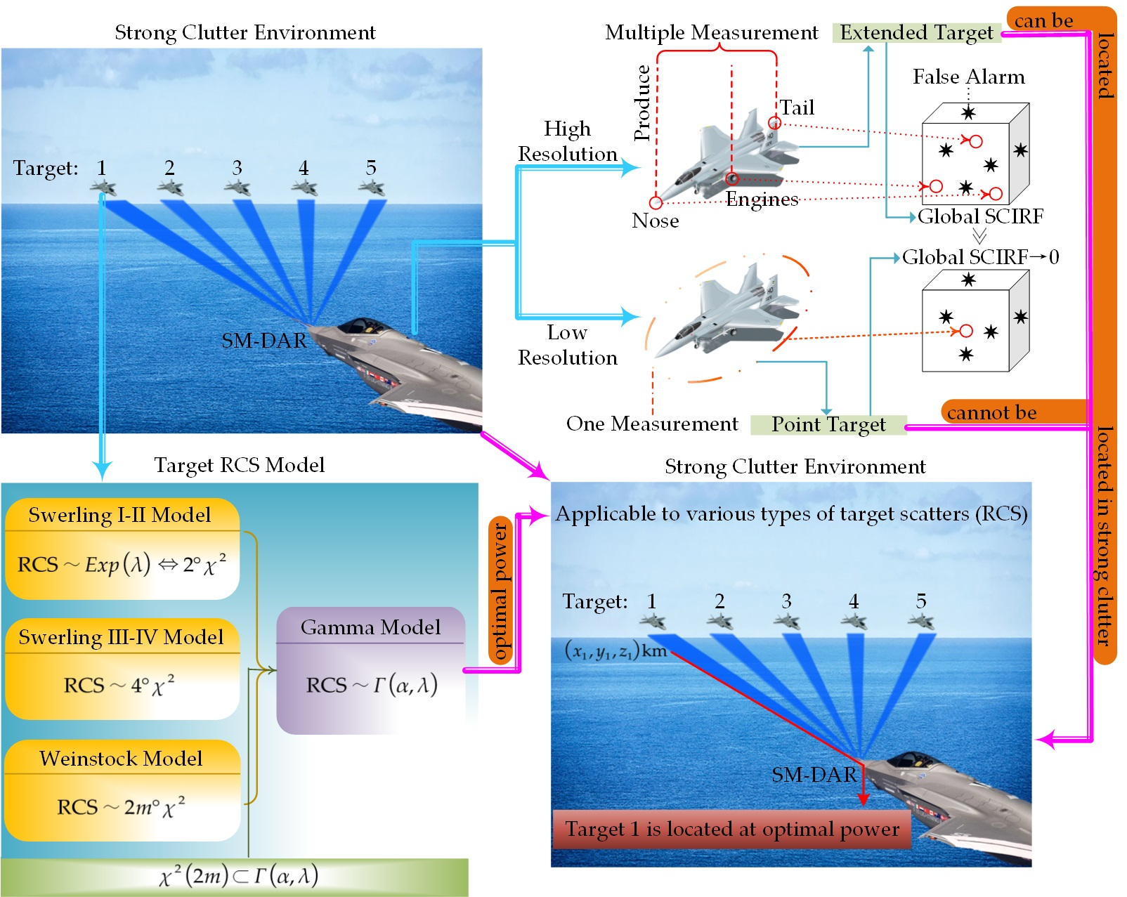
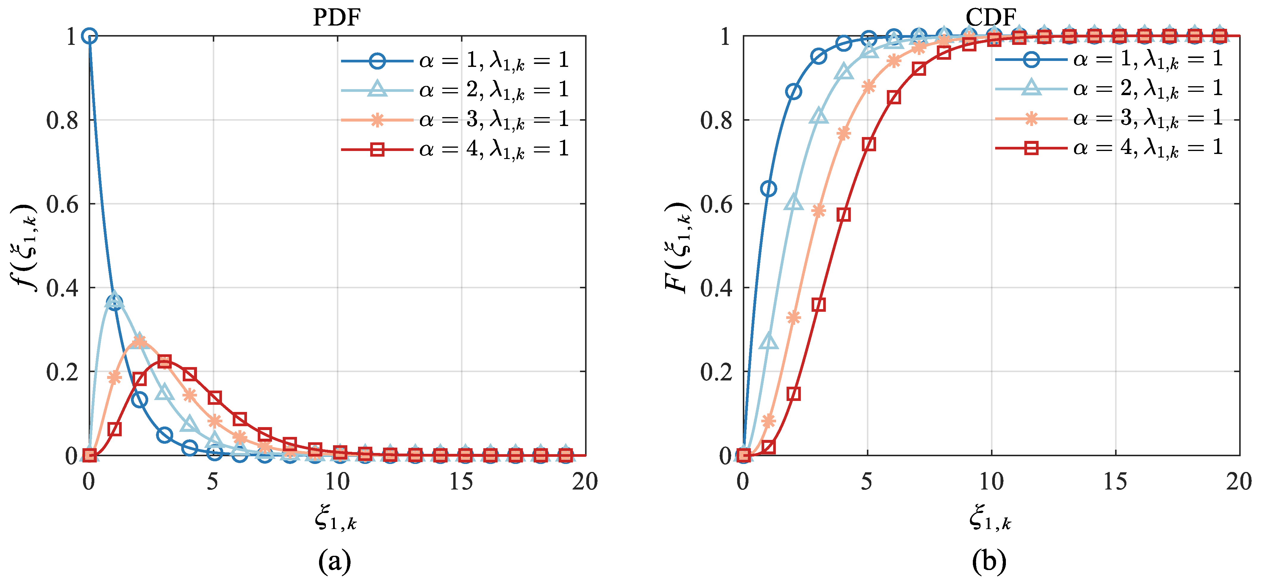
- The relationship between the shape parameter and target localization power allocation of target RCS with Gamma distribution law in strong clutter is deeply excavated. At the same confidence level, the power consumption of the target decreases with the increase in the shape parameter. The reason is that when the shape parameter with a larger value causes its cumulative probability to approach 1 to slow down, the probability of RCS taking a larger value in the definition domain will increase, so the negative correlation between RCS and target power consumption makes the relationship between target power consumption and shape parameter also negative correlation. At the same time, the Gamma target model proposed in this paper covers the Swerling I–IV model and the Weinstock model, and the distribution between the generalized chi-square distribution and the Gamma distribution. This type of distribution can often more accurately describe the complex RCS dynamic statistical characteristics of stealth targets, reflecting the universality of the Gamma distribution target model. In addition, from a mathematical point of view, making the RCS obey the Gamma distribution can not only mathematically process many target models uniformly but also physically fit the complex RCS dynamic statistical characteristics of various stealth targets convenient for engineering applications.
2. System Model and Preliminaries
2.1. RCS Model
2.2. Measurement Model
2.3. Theory of Extended Target
2.3.1. Probability Distribution of
2.3.2. Probability Distribution of Measurement Number Originating from Target
2.4. Theory of Clutter
2.4.1. Spatial Distribution of False Alarm on Clutter
2.4.2. Number Distribution of False Alarm on Clutter
3. Construction of Extended Robust Chance-Constrained Power Allocation Scheme
3.1. Derivation of Probability Density Function of Measurement Vector
3.1.1. Distribution That Target Is Detected
3.1.2. Distribution of Number of Targets Passing Threshold
3.1.3. Probability of Measurement from Target q
3.1.4. Probability Density Function of Measurement
3.2. Evaluation of Multiple Extended Target Localization Performance in Strong Clutter
3.2.1. Calculation of Conditional Fisher Information Matrix in Strong Clutter
3.2.2. Calculation of Fisher Information Matrix in Strong Clutter
3.2.3. Constraints Construction of Pcrlb for Multi-Target Localization in Strong Clutter
3.3. Gamma Chance-Constrained Programming Model
3.4. Solution of Γ-CCP Model
3.4.1. Equivalent Representation of Problem
3.4.2. Analytic Solution and Numerical Solution of -CCP Model
| Algorithm 1: Detailed steps of the extended numerical algorithm |
 |
4. Simulation
4.1. Information Reduction Factor in Clutter
4.1.1. Calculation of Scirf Based on Monte Carlo Method
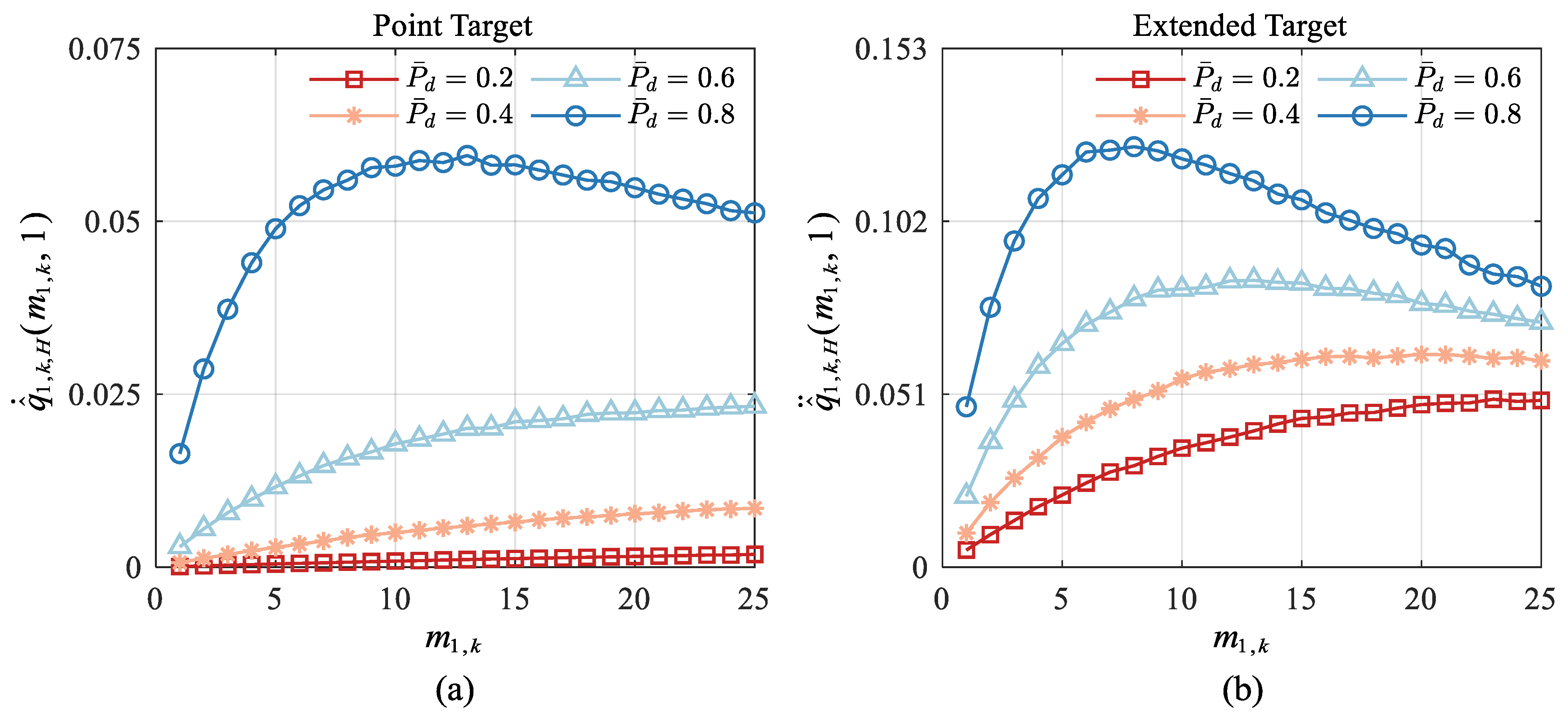
4.1.2. Comparison among with Different
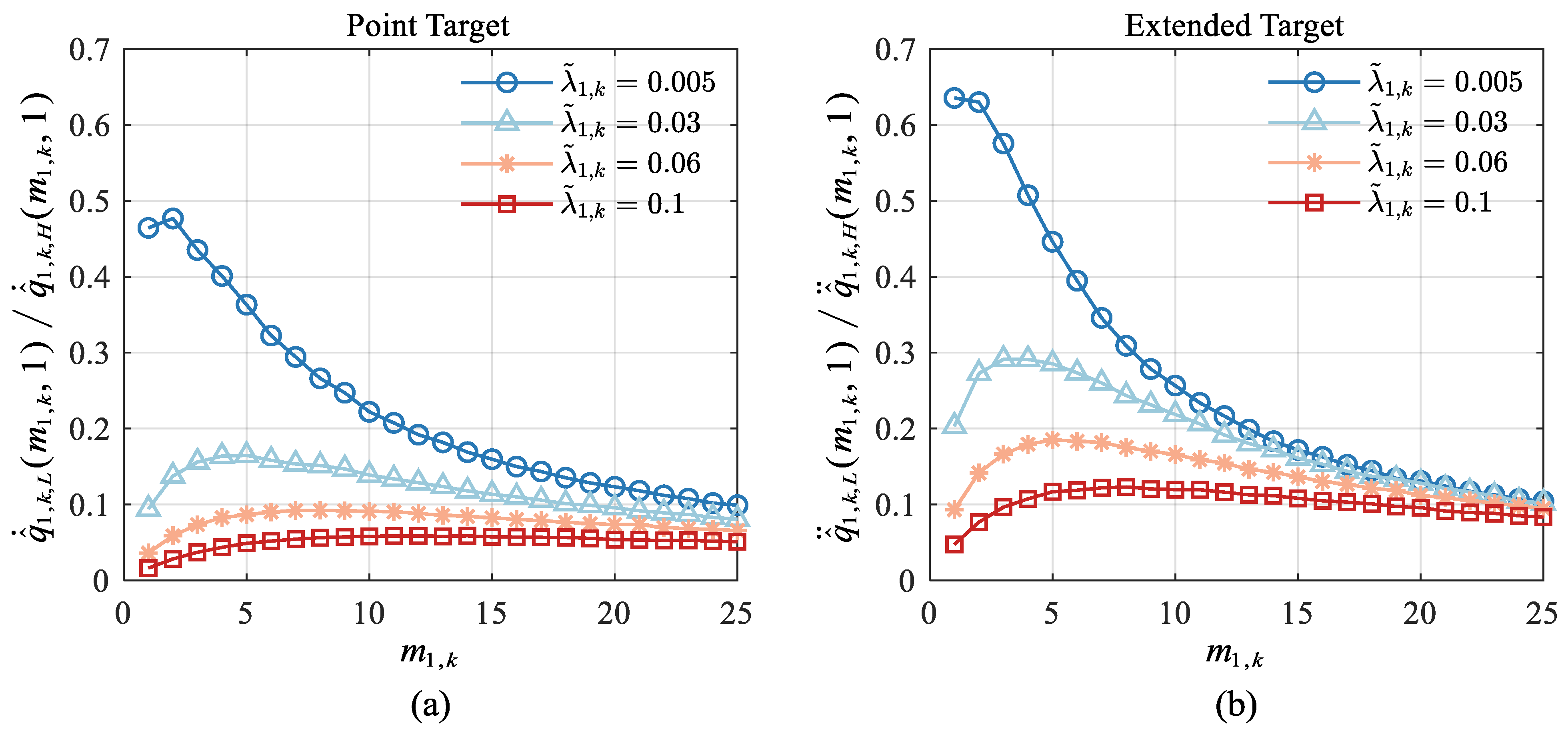
4.1.3. Comparison among with Different
4.1.4. Global IRF and Global SCIRF under Different Detection Probability
4.2. Verification of Effectiveness of ERCC-PA Scheme
4.2.1. Power Allocation of Case1: Swerling I and II
4.2.2. Power Allocation of Case2: Swerling III and IV, Case3 and Case4
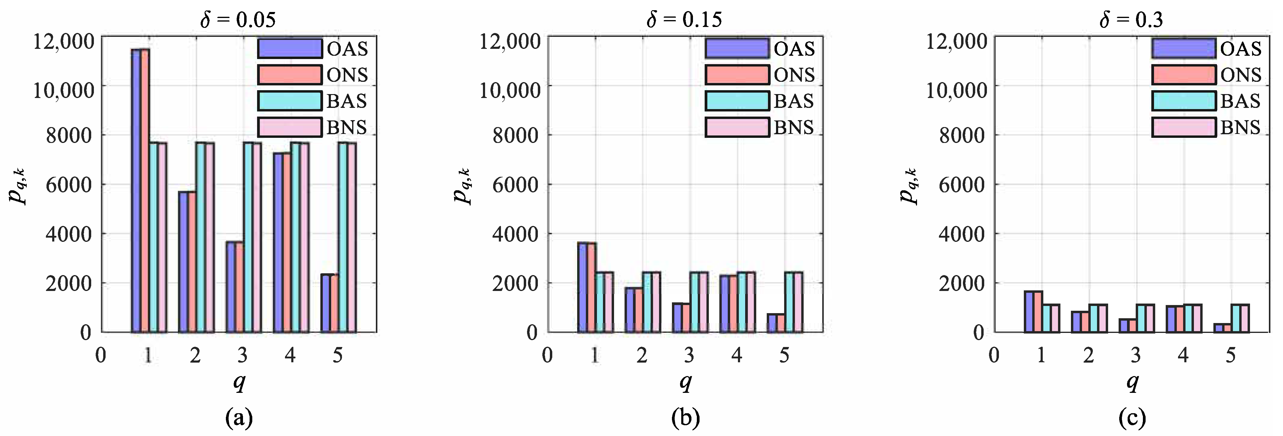
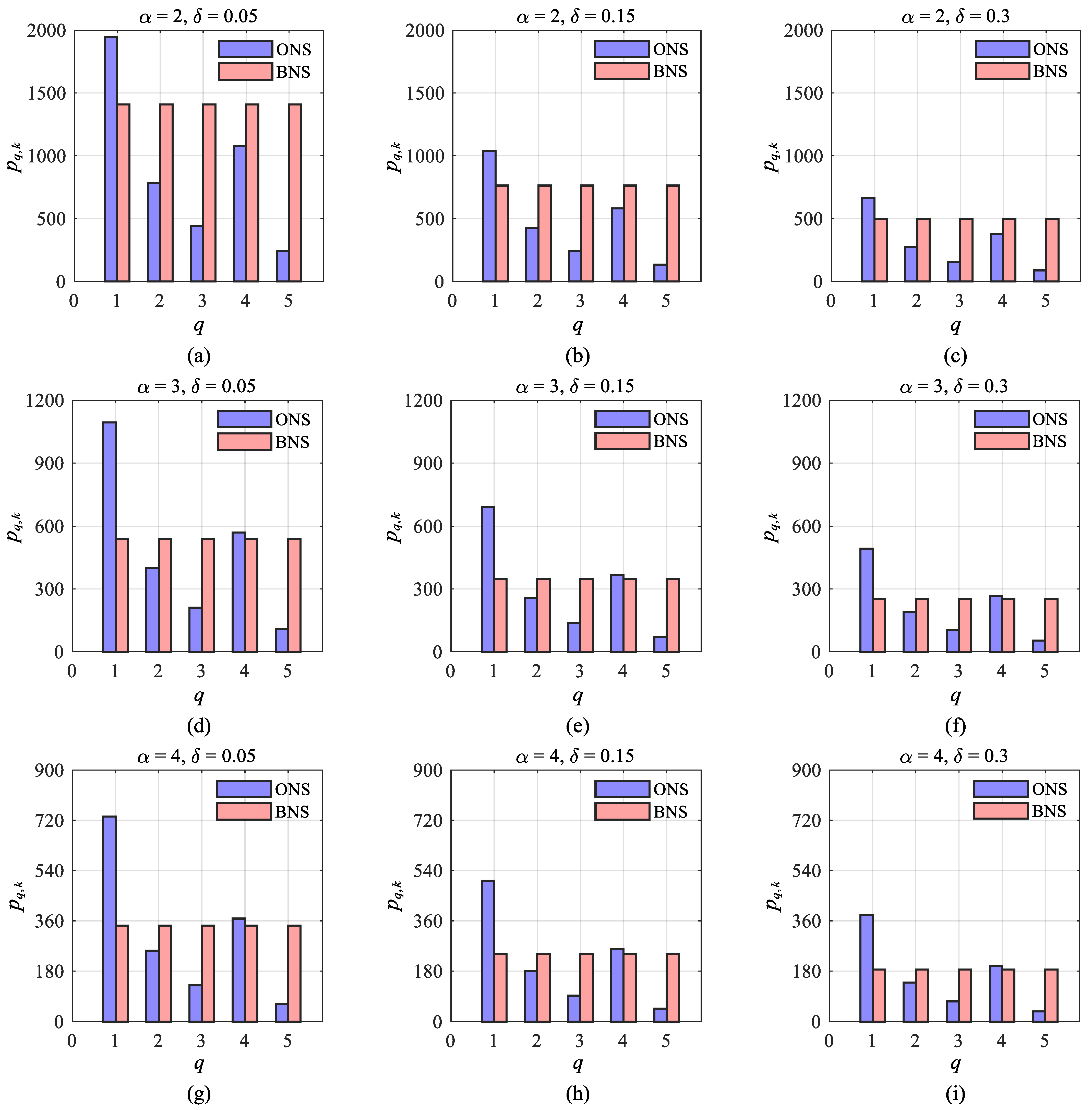
- When the target number of RCSs with the same expectation is , more power resources can be allocated to the farther targets (such as the allocation results of Target 1 and Target 4);
- Under the condition that the number of targets with the same distance is , more power resources are allocated to the target with a smaller average RCS (such as the allocation results of Target 3 and Target 5).
4.3. Robustness of ERCC-PA Scheme
4.3.1. Verification of Robustness of the ERCC-PA Scheme
4.3.2. Metrics of Robustness of the ERCC-PA Scheme
5. Conclusions
Author Contributions
Funding
Data Availability Statement
Conflicts of Interest
Appendix A. Nomenclature

| Parameter | Definition |
|---|---|
| Probability value | |
| Cumulative Distribution Function (CDF) | |
| Probability Density Function for continuous random variables (PDF) | |
| Probability Mass Function for discrete random variables (PMF) | |
| State vector of target q at time k | |
| Dimension of | |
| Observation vector of at time k | |
| The jth index in | |
| Error standard deviation of | |
| Number of all measurements within the threshold of target q at time k | |
| Number of real targets measured within the threshold of target q at time k | |
| Number of false alarms measured within the threshold of target q at time k | |
| Number of combinations given and , i.e., | |
| Random measurement vector group, i.e., | |
| The ith measurement | |
| The ith measurement is the real target | |
| The ith measurement is false alarm | |
| Dimensions of , , and | |
| Values of all measurements, i.e | |
| Value of , i.e., | |
| Value of , i.e., | |
| Value of , i.e., | |
| The jth component of , i.e., one-dimensional random variable | |
| The jth component of , i.e., one-dimensional random variable | |
| The jth component of , i.e., one-dimensional random variable | |
| Value of , i.e., | |
| Value of , i.e., | |
| Value of , i.e., | |
| The ith measurement in the kth combination when the combination number is | |
| In the kth combination with combination number , the ith measurement is the real target | |
| In the kth combination with combination number , the ith measurement is the false alarm | |
| Value of , i.e., | |
| Value of , i.e., | |
| Value of , i.e., | |
| Probability that measurement contains point target q’s measurement. | |
| Probability that measurement contains extended target q’s measurement. | |
| IRF of point target q | |
| IRF of extended target q. | |
| Global IRF of point target q. | |
| Global IRF of extended target q. |
Appendix B. Proof of Global SCIRF for Extended Targets
- Assumption A1. To reduce the amount of calculation, the measurement is limited to a certain threshold as below,where denotes the jth component of the measured value , represents the jth component of , and is the jth component’s error standard deviation of the measured vector.
- Assumption A2. The dimensions of the measured values are orthogonal to each other, then A can be represented by a hypercubeand the hypercube’s volume is
Appendix C. Proof of the Convexity for the Optimization Problem
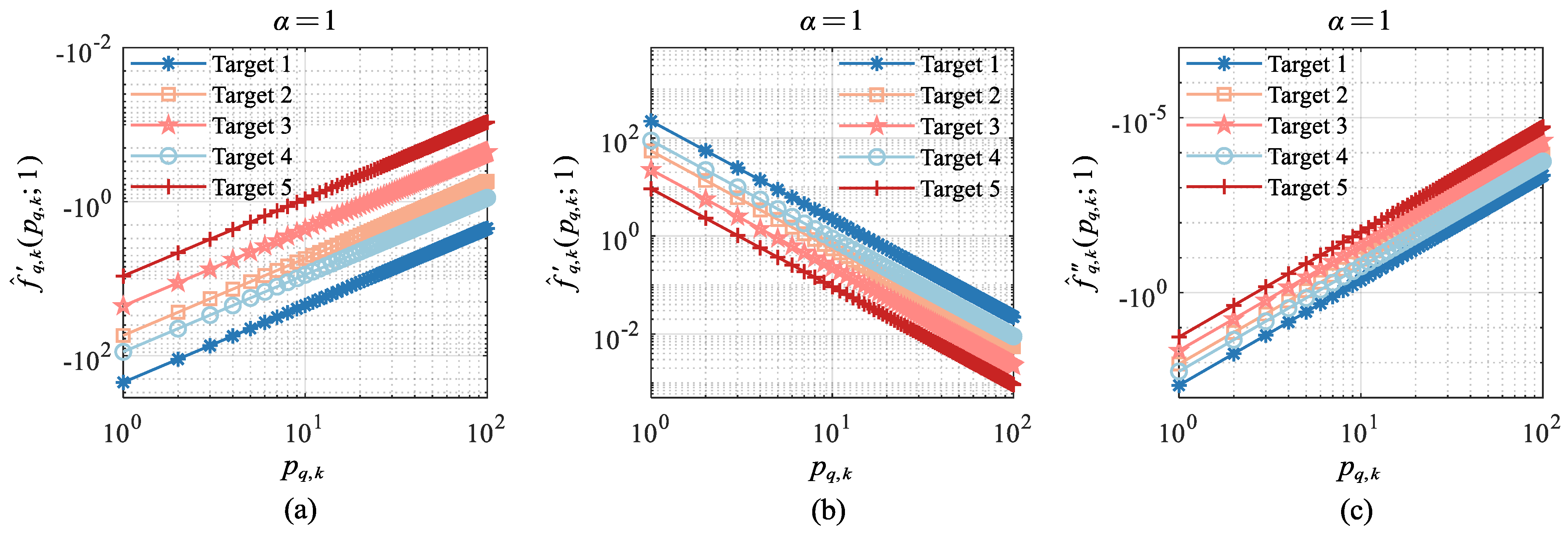
- (1)
- For all shape parameters , is a monotone increasing function of ;
- (2)
- For all shape parameters , is a monotone decreasing function of ;
- (3)
- For all shape parameters , the Hessian matrix is negative definite, which means that the constraint function is concave.
Appendix D. Size Relationship between and When
Appendix E. Size Relationship between and When n1,k = 1
References
- Yan, J.K.; Liu, H.W.; Jiu, B.; Chen, B.; Liu, Z.; Bao, Z. Simultaneous multibeam resource allocation scheme for multiple target tracking. IEEE Trans. Signal Process. 2015, 63, 3110–3122. [Google Scholar] [CrossRef]
- Chen, X.Z.; Shu, T.; Yu, K.B.; Zhang, Y.; Lei, Z.Y.; He, J.; Yu, W.X. Implementation of an adaptive wideband digital array radar processor using subbanding for enhanced jamming cancellation. IEEE Trans. Aerosp. Electron. Syst. 2020, 57, 762–775. [Google Scholar] [CrossRef]
- Williamson, T.G.; Whelan, J.; Disharoon, W.; Simmons, P.; Houck, J.; Holman, B.; Alward, J.; McDonald, K.; Kim, S.; Andreasen, D.; et al. Techniques for digital array radar planar near-field calibration by retrofit of an analog system. In Proceedings of the 2021 IEEE Radar Conference (RadarConf21), Atlanta, GA, USA, 7–14 May 2021; pp. 1–6. [Google Scholar]
- Cheng, T.; Li, Z.Z.; Tan, Q.Q.; Wang, S.X.; Yue, C.Y. Real-time Adaptive Dwell Scheduling for Digital Array Radar based on Virtual Dynamic Template. IEEE Trans. Aerosp. Electron. Syst. 2022, 58, 3197–3208. [Google Scholar] [CrossRef]
- Godrich, H.; Petropulu, A.P.; Poor, H.V. Power allocation strategies for target localization in distributed multiple-radar architectures. IEEE Trans. Signal Process. 2011, 59, 3226–3240. [Google Scholar] [CrossRef]
- Tichavsky, P.; Muravchik, C.H.; Nehorai, A. Posterior Cramér-Rao bounds for discrete-time nonlinear filtering. IEEE Trans. Signal Process. 1998, 46, 1386–1396. [Google Scholar] [CrossRef] [Green Version]
- Hernandez, M.L.; Farina, A.; Ristic, B. PCRLB for tracking in cluttered environments: Measurement sequence conditioning approach. IEEE Trans. Aerosp. Electron. Syst. 2006, 42, 680–704. [Google Scholar] [CrossRef]
- Hernandez, M.; Benavoli, A.; Graziano, A.; Farina, A.; Morelande, M. Performance measures and MHT for tracking move-stop-move targets with MTI sensors. IEEE Trans. Aerosp. Electron. Syst. 2011, 47, 996–1025. [Google Scholar] [CrossRef]
- Su, Y.; Cheng, T.; He, Z.S.; Lu, X.J. Joint Detection Threshold Optimization and Transmit Resource Allocation for Targets Tracking in Clutter with Colocated MIMO Radar Networks. In Proceedings of the 2022 25th International Conference on Information Fusion (FUSION), Linköping, Sweden, 4–7 July 2022; pp. 1–7. [Google Scholar]
- Sun, H.; Li, M.; Zuo, L.; Cao, R.Q. Joint threshold optimization and power allocation of cognitive radar network for target tracking in clutter. Signal Process. 2020, 172, 107566. [Google Scholar] [CrossRef]
- Zhang, H.W.; Liu, W.J.; Zhang, Z.J.; Lu, W.L.; Xie, J.W. Joint target assignment and power allocation in multiple distributed MIMO radar networks. IEEE Syst. J. 2020, 15, 694–704. [Google Scholar] [CrossRef]
- Han, Q.H.; Pan, M.H.; Liang, Z.H. Joint power and beam allocation of opportunistic array radar for multiple target tracking in clutter. Digit. Signal Process. 2018, 78, 136–151. [Google Scholar] [CrossRef]
- Yan, J.K.; Liu, H.W.; Bao, Z. Power allocation scheme for target tracking in clutter with multiple radar system. Signal Process. 2018, 144, 453–458. [Google Scholar] [CrossRef]
- Tuncer, B.; Özkan, E. Random matrix based extended target tracking with orientation: A new model and inference. IEEE Trans. Signal Process. 2021, 69, 1910–1923. [Google Scholar] [CrossRef]
- Yao, Y.; Liu, H.T.; Miao, P.; Wu, L. MIMO radar design for extended target detection in a spectrally crowded environment. IEEE Trans. Intell. Transp. Syst. 2021, 23, 14389–14398. [Google Scholar] [CrossRef]
- Lian, F.; Wang, T.T.; Han, C.Z.; Zhang, G.H. PCRLB for Extended Target Tracking. Control and Decision 2016. Available online: http://kzyjc.alljournals.cn/kzyjc/article/abstract/2015-0630?st=article_issue (accessed on 20 August 2016).
- Yan, J.K.; Liu, H.W.; Jiu, B.; Bao, Z. Power allocation algorithm for target tracking in unmodulated continuous wave radar network. IEEE Sens. J. 2014, 15, 1098–1108. [Google Scholar]
- Shi, C.G.; Wang, Y.J.; Wang, F.; Salous, S.; Zhou, J.J. Joint optimization scheme for subcarrier selection and power allocation in multicarrier dual-function radar-communication system. IEEE Syst. J. 2020, 15, 947–958. [Google Scholar] [CrossRef]
- Zhang, H.W.; Liu, W.J.; Fei, T.Y. Joint detection threshold adjustment and power allocation strategy for cognitive MIMO radar target tracking. Digit. Signal Process. 2022, 126, 103379. [Google Scholar] [CrossRef]
- Yan, J.K.; Pu, W.Q.; Zhou, S.H.; Liu, H.W.; Bao, Z. Collaborative detection and power allocation framework for target tracking in multiple radar system. Inf. Fusion 2020, 55, 173–183. [Google Scholar] [CrossRef]
- Shi, C.G.; Wang, F.; Salous, S.; Zhou, J.J. Joint subcarrier assignment and power allocation strategy for integrated radar and communications system based on power minimization. IEEE Sens. J. 2019, 19, 11167–11179. [Google Scholar] [CrossRef]
- Zhang, H.W.; Liu, W.J.; Zong, B.F.; Shi, J.P.; Xie, J.W. An efficient power allocation strategy for maneuvering target tracking in cognitive MIMO radar. IEEE Trans. Signal Process. 2021, 69, 1591–1602. [Google Scholar] [CrossRef]
- Skolnik, M.I. Theoretical Accuracy of Radar Measurements. IRE Trans. Aeronaut. Navig. Electron. 1960, ANE-7, 123–129. [Google Scholar] [CrossRef]
- Yan, J.K.; Liu, H.W.; Pu, W.Q.; Zhou, S.H.; Liu, Z.; Bao, Z. Joint beam selection and power allocation for multiple target tracking in netted colocated MIMO radar system. IEEE Trans. Signal Process. 2016, 64, 6417–6427. [Google Scholar] [CrossRef]
- Swerling, P. Probability of detection for fluctuating targets. IRE Trans. Inf. Theory 1960, 6, 269–308. [Google Scholar] [CrossRef]
- Zhang, Y.S.; Pan, M.H.; Han, Q.H. Joint sensor selection and power allocation algorithm for multiple-target tracking of unmanned cluster based on fuzzy logic reasoning. Sensors 2020, 20, 1371. [Google Scholar] [CrossRef] [PubMed] [Green Version]
- Fang, Z.X.; Wei, Z.Q.; Chen, X.; Wu, H.C.; Feng, Z.Y. Stochastic geometry for automotive radar interference with RCS characteristics. IEEE Wirel. Commun. Lett. 2020, 9, 1817–1820. [Google Scholar] [CrossRef]
- Han, Q.H.; Pan, M.H.; Long, W.J.; Liang, Z.H.; Shan, C.G. Joint Adaptive Sampling Interval and Power Allocation for Maneuvering Target Tracking in a Multiple Opportunistic Array Radar System. Sensors 2020, 20, 981. [Google Scholar] [CrossRef] [PubMed] [Green Version]
- Rashid, U.; Tuan, H.D.; Apkarian, P.; Kha, H.H. Globally optimized power allocation in multiple sensor fusion for linear and nonlinear networks. IEEE Trans. Signal Process. 2011, 60, 903–915. [Google Scholar] [CrossRef]
- Chavali, P.; Nehorai, A. Scheduling and power allocation in a cognitive radar network for multiple-target tracking. IEEE Trans. Signal Process. 2011, 60, 715–729. [Google Scholar] [CrossRef]
- Yan, J.K.; Pu, W.Q.; Liu, H.W.; Jiu, B.; Bao, Z. Robust chance constrained power allocation scheme for multiple target localization in colocated MIMO radar system. IEEE Trans. Signal Process. 2018, 66, 3946–3957. [Google Scholar] [CrossRef]
- Charnes, A.; Cooper, W.W. Chance-constrained programming. Manag. Sci. 1959, 6, 73–79. [Google Scholar] [CrossRef]
- Trees, V.; Harry, L. Detection, Estimation, and Modulation Theory-Part III; John Wiley & Sons: New York, NY, USA, 2001. [Google Scholar]
- Richards, M.A. Fundamentals of Radar Signal Processing; McGraw-Hill Education: New York, NY, USA, 2014. [Google Scholar]
- Gilholm, K.; Drummond, O.E.; Godsill, S.; Maskell, S.; Salmond, D. Poisson models for extended target and group tracking. In Signal and Data Processing of Small Targets 2005; SPIE: Bellingham, WA, USA, 2005; pp. 230–241. [Google Scholar]
- Mukhopadhyay, N. Probability and Statistical Inference; CRC Press: Boca Raton, FL, USA, 2020. [Google Scholar]
- Song, X.F.; Willett, P.; Zhou, S.L. On Fisher information reduction for range-only localization with imperfect detection. IEEE Trans. Aerosp. Electron. Syst. 2012, 48, 3694–3702. [Google Scholar] [CrossRef]
- Trees, H.L.V.; Bell, K.L. Bayesian Bounds for Parameter Estimation and Nonlinear Filtering/Tracking; Wiley-IEEE Press: New York, NY, USA, 2007; pp. 2–85. [Google Scholar]
- Li, Z.; Liu, H.; Zhang, Z.; Liu, T.; Xiong, N.N. Learning knowledge graph embedding with heterogeneous relation attention networks. IEEE Trans. Neural Netw. Learn. Syst. 2021, 33, 3961–3973. [Google Scholar] [CrossRef] [PubMed]
- Liu, H.; Liu, T.; Zhang, Z.; Sangaiah, A.K.; Yang, B.; Li, Y. Arhpe: Asymmetric relation-aware representation learning for head pose estimation in industrial human–computer interaction. IEEE Trans. Ind. Inform. 2022, 18, 7107–7117. [Google Scholar] [CrossRef]
- Liu, H.; Liu, T.; Chen, Y.; Zhang, Z.; Li, Y.F. EHPE: Skeleton cues-based gaussian coordinate encoding for efficient human pose estimation. IEEE Trans. Multimed. 2022, 1–12. [Google Scholar] [CrossRef]


| Swerling I–II | Swerling III–IV | Weinstock | ||
|---|---|---|---|---|
| Case1 () | Case2 () | Case3 () | Case4 () | |
| Degree of polynomial Equation | 2 | 3 | 4 | 5 |
| Transcendental Function * | Y ** | F ** | F | F |
| Existence of analytical solution of | Y ** | F ** | F | F |
| Parameter Symbol | Value | Meaning |
|---|---|---|
| 0.8 | Probability of detection | |
| Probability of false alarm | ||
| 2 Mhz | Beam width of receiver antenna | |
| 1 | Effective bandwidth | |
| 2 | Expectation of the number of measurement values from the target | |
| g | 4 | Gate coefficient |
| 400 | Volume of tracking gate | |
| Monte Carlo simulation times |
| Target Number | 1 | 2 | 3 | 4 | 5 | |
|---|---|---|---|---|---|---|
| Target Index & Symbol | ||||||
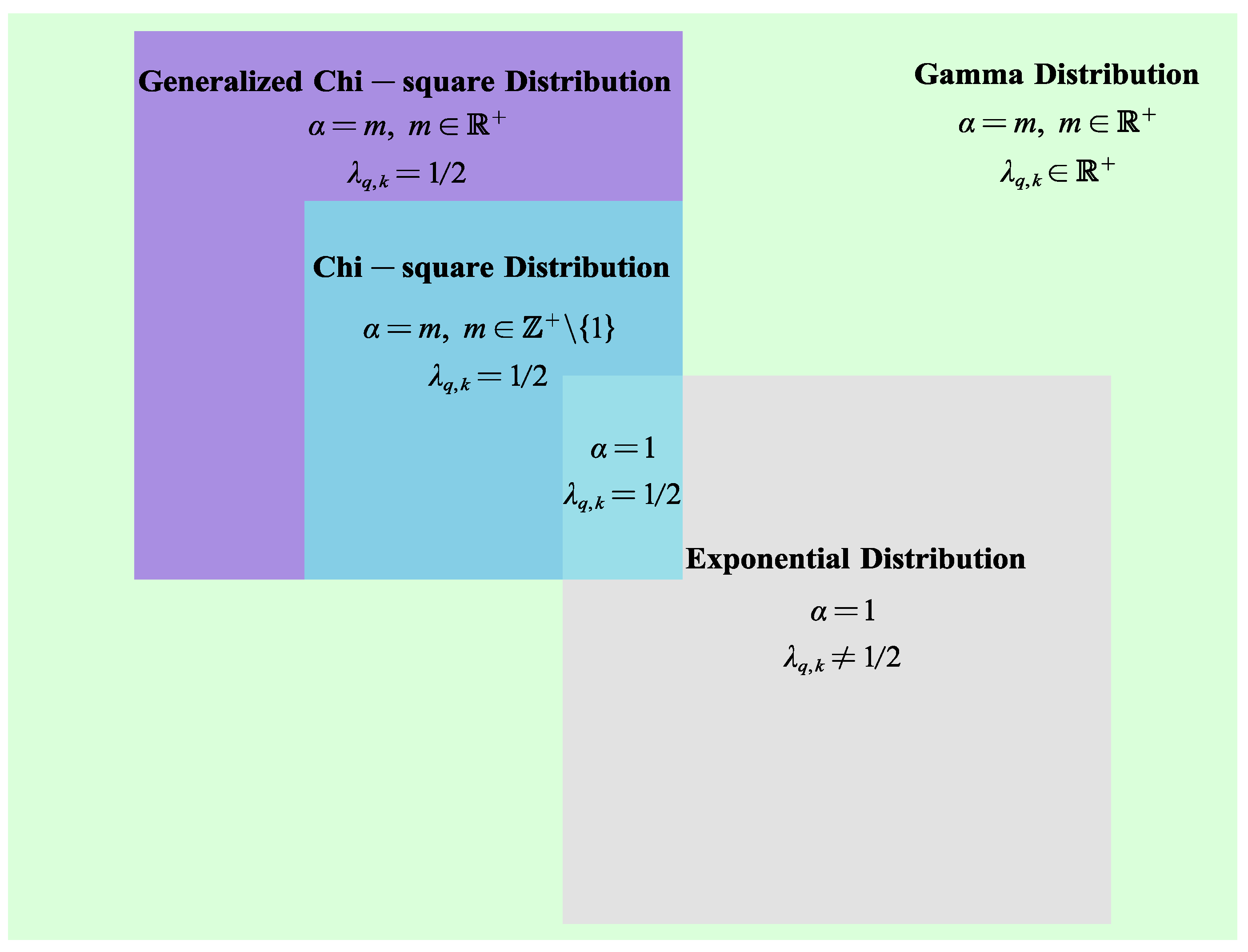
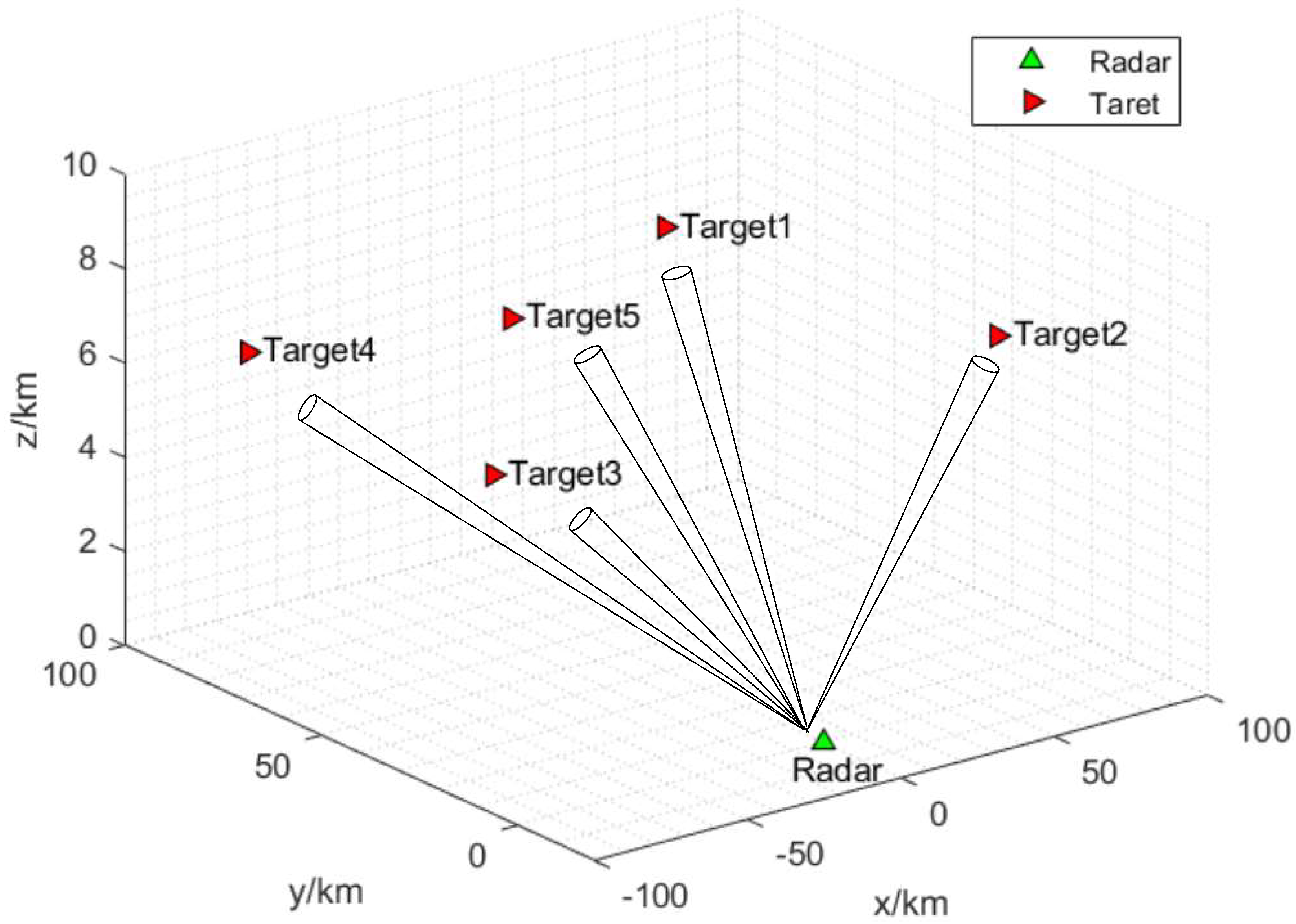
| Position (km) & | (71.5, 96.4, 6) | (91.1, 27, 6) | (−74.6, 26, 6) | (−70, 92, 6) | (−1, 79, 6) | |
| Distance (km) & | 120 | 95 | 79 | 115.6 | 79 | |
| Threshold of PCRLB (m) & | 500 | 500 | 500 | 500 | 500 | |
| Expectation of RCS & | 1 | 1 | 0.8 | 2 | 2 | |
| Parameter Name | Symbol | Value | |||||
|---|---|---|---|---|---|---|---|
| Detection Probability | 0.3 | 0.4 | 0.5 | 0.6 | 0.7 | 0.8 | |
| Global SCIRF | 0.0009 | 0.0053 | 0.0155 | 0.0525 | 0.2532 | 0.9331 | |
| Parameter Name | Symbol | Value | |||||
|---|---|---|---|---|---|---|---|
| Detection Probability | 0.3 | 0.4 | 0.5 | 0.6 | 0.7 | 0.8 | |
| Global IRF | 0.0227 | 0.0648 | 0.1460 | 0.2920 | 0.5268 | 0.8986 | |
| Indicator | Case1 | Case2 | Case3 | Case4 | ||
|---|---|---|---|---|---|---|
| OAS | ONS | ONS | ONS | ONS | ||
| 0.95 | 30,410.7 | 30,410.7 | 4169.1 | 2383.7 | 1719.9 | |
| 0.85 | 8898.4 | 8898.4 | 2248.1 | 1524.1 | 1197.8 | |
| 0.70 | 4054.5 | 4054.5 | 1451.9 | 1102.8 | 918.8 | |
| Case1 | Case2 | Case3 | Case4 | ||
|---|---|---|---|---|---|
| OAS | ONS | ONS | ONS | ONS | |
| 0.95 | 20.91% | 20.65% | 36.24% | 11.38% | 9.56% |
| 0.85 | 20.91% | 20.92% | 36.61% | 12.06% | 10.36% |
| 0.70 | 20.91% | 20.87% | 36.96% | 12.69% | 11.07% |
| Case1 | Case2 | Case3 | Case4 | ||
|---|---|---|---|---|---|
| OAS | ONS | ONS | ONS | ONS | |
| 0.95 | 0.9503 | 0.9498 | 0.9503 | 0.9502 | 0.9504 |
| 0.85 | 0.8504 | 0.8495 | 0.8501 | 0.8503 | 0.8503 |
| 0.70 | 0.7103 | 0.7000 | 0.7002 | 0.6996 | 0.6999 |
| Indicator | Case1 | Case2 | Case3 | Case4 | ||
|---|---|---|---|---|---|---|
| OAS | ONS | ONS | ONS | ONS | ||
| 0.95 | 0.48% | 0.48% | 0.60% | 0.49% | 0.74% | |
| 0.85 | 0.25% | 0.25% | 0.13% | 0.22% | 0.22% | |
| 0.70 | 0.01% | 0.01% | 0.07% | 0.14% | 0.04% | |
Disclaimer/Publisher’s Note: The statements, opinions and data contained in all publications are solely those of the individual author(s) and contributor(s) and not of MDPI and/or the editor(s). MDPI and/or the editor(s) disclaim responsibility for any injury to people or property resulting from any ideas, methods, instructions or products referred to in the content. |
© 2023 by the authors. Licensee MDPI, Basel, Switzerland. This article is an open access article distributed under the terms and conditions of the Creative Commons Attribution (CC BY) license (https://creativecommons.org/licenses/by/4.0/).
Share and Cite
Xue, C.; Wang, L.; Zhu, D. An Extended Robust Chance-Constrained Power Allocation Scheme for Multiple Target Localization of Digital Array Radar in Strong Clutter Environments. Remote Sens. 2023, 15, 1267. https://doi.org/10.3390/rs15051267
Xue C, Wang L, Zhu D. An Extended Robust Chance-Constrained Power Allocation Scheme for Multiple Target Localization of Digital Array Radar in Strong Clutter Environments. Remote Sensing. 2023; 15(5):1267. https://doi.org/10.3390/rs15051267
Chicago/Turabian StyleXue, Chenyan, Ling Wang, and Daiyin Zhu. 2023. "An Extended Robust Chance-Constrained Power Allocation Scheme for Multiple Target Localization of Digital Array Radar in Strong Clutter Environments" Remote Sensing 15, no. 5: 1267. https://doi.org/10.3390/rs15051267