
Impacts of Extreme Climates on Vegetation at Middle-to-High Latitudes in Asia

1
Key Laboratory of Meteorological Disaster, Ministry of Education, Joint International Research Laboratory of Climate and Environment Change (ILCEC), Collaborative Innovation Center on Forecast and Evaluation of Meteorological Disasters, Nanjing University of Information Science & Technology (NUIST), Nanjing 210044, China
2
School of Atmospheric Sciences, Nanjing University of Information Science and Technology, Nanjing 210044, China
*
Author to whom correspondence should be addressed.
Remote Sens. 2023, 15(5), 1251; https://doi.org/10.3390/rs15051251
Submission received: 2 January 2023
/
Revised: 8 February 2023
/
Accepted: 21 February 2023
/
Published: 24 February 2023
(This article belongs to the Special Issue Vegetation Dynamics Revealed by Remote Sensing and Its Feedback to Regional and Global Climate Ⅱ)
Abstract
:In this study, we investigated the synchronous responses of vegetation to extreme temperatures and/or precipitation at middle-to-high latitudes in Asia using semi-monthly observations of the GIMMS and GLASS leaf area index (LAI) from 1982 to 2016. The extreme vegetation and climate states were specified using standard anomalies of the annual cycle with removed variables. The results show that the area with the maximum or minimum LAI increased or decreased in correspondence with global warming. Both the GIMMS and GLASS LAI mostly reached their maximum in spring and autumn. The GIMMS LAI mostly reached its minimum in summer, while the GLASS LAI mostly reached its minimum in late spring or late summer. The GIMMS and GLASS datasets were generally consistent regarding the vegetation responses to extreme temperatures and precipitation, especially in the areas covered by trees. Extreme cold and/or wet conditions inhibited forest growth in the area south of 60 °N, particularly from October to November. Extreme hot and/or dry conditions promoted forest growth, particularly in the central and northern parts of Siberia from August to September. However, in some arid areas of Central Asia and the Mongolian Highlands, which are mostly covered by sparse vegetation and grasses, low temperature extremes and/or strong precipitation promoted vegetation growth, while high temperature extremes and/or low precipitation had adverse effects on vegetation growth. This was more apparent in the GIMMS LAI than it was in the GLASS LAI, since the GIMMS dataset supplied more values representing extreme states of vegetation. The compound extreme of hot-and-dry and cold-and-wet climates were more frequent than the combination of cold and dry climates and hot-and-wet climates were. The overall positive response of the vegetation was superior to the negative response. The results of this study suggest that a continuous increase in vegetation density and coverage will occur over the boreal region in the future if the warming trend persists. The consequent climate feedback in this area on the regional and global scales should be afforded more attention.
1. Introduction
Climate change is one of humanity’s greatest challenges in the 21st Century [1]. The global 2 m temperature increased by 1.53 ± 0.15 ℃ from 1850–1900 to 2006–2015, and this trend may become more prominent in the coming decades [2]. Along with the warming trend, most terrestrial areas have experienced an increase in the number of warm and hot nights and a decrease in the number of cold days and nights [3]. The frequency and intensity of the observed heat-related events have also significantly increased [3]. In future decades, 50–80% of the land area is projected to undergo more heat events than those that are observed in the present day [4]. Although the long-term trend of global droughts are still a controversial problem due to natural variability, potential deficiencies in drought indices, uncertainty regarding the quality of the precipitation data, and changes in the frequency and intensity of droughts are evident in some regional areas [5,6,7,8]. A recent global analysis of a dataset encompassing 4500 meteorological sites found an increase in the drought frequency affecting the east coast of the USA, Amazonia, northeastern Brazil, Patagonia, the Mediterranean region, north-eastern China, and most parts of Africa, while a decrease was observed in northern Argentina, Uruguay, and Northern Europe [9]. Global warming intensifies the hydrological cycle and affects extreme regional precipitation events [10,11]. During 1981–2010, the global number of record-breaking rainfall events increased significantly by 12% compared to the expected figure due to multi-decadal climate variability [12].
Extreme compound events have also gained increasing attention from the scientific community and climate researchers. The Intergovernmental Panel on Climate Change Sixth Assessment Report [13] reported that the number of compound dry–hot events observed worldwide has increased since the 1950s. This increasing trend is projected to continue with high probability if global warming persists in the future [13]. In particular, compound dry–hot events are likely to occur more frequently in northern Eurasia, Europe, southeastern Australia, the United States, India, and northwestern China [14]. During 2021, China, Germany, and Bangladesh experienced severe floods; Australia and British Columbia experienced record-breaking wildfires; severe heat waves occurred in Siberia, extending to the Death Valley; Japan and Texas experienced destructive typhoons [15]. Therefore, it is necessary to understand the consequent damage and disasters related to extreme weather and climatic events.
The impacts of extreme climate and weather events on terrestrial ecosystems have attracted the interest and attention of researchers worldwide [16,17]. Terrestrial vegetation is a vital component of ecosystems and forms the natural bond between land and atmosphere [18]. Climate states and variability influence variation in ecosystems [19,20]. In general, warm climates promote vegetation growth when energy is the limiting factor for vegetation growth; however, extremely hot climates may inhibit vegetation growth by influencing plant metabolism and cell integrity when water is the limiting factor [21,22,23,24,25]. The impacts of extreme cold events on ecosystems have also been investigated [26]. Studies have suggested that extreme cold events during the growing season weaken the water absorption capacity of vegetation, which slows their growth. Furthermore, cell dehydration caused by freezing can lead to freezing injuries and even the death of plant tissues [27,28]. Although the number of frost days has decreased in recent decades [29], this decrease does not always occur during the vegetation growing period. Significant increases have been observed in some areas, such as Europe. This is because of the longer vegetation growing season due to climate warming [30]. The influence of extreme precipitation on ecosystems mainly depends on the water conditions of the ecosystem during extreme precipitation events [31]. In arid regions, extreme precipitation increases the soil moisture, further increasing ecosystem productivity and carbon accumulation. However, in humid regions, extreme precipitation can impede ecosystem carbon sequestration [32]. Many studies have consistently concluded that droughts reduce the greenness of vegetation, significantly weaken the carbon sink function of ecosystems, and even cause terrestrial ecosystems to switch from a carbon sink to a carbon source [33,34,35,36].
Areas at high latitudes are characterized by short growing seasons due to long, cold winters and the persistence of snow [37]. However, since the Industrial Revolution, the warming trend has affected the high latitudes of Eurasia the most [38], with the area experiencing an increase in extreme heat. A warmer climate generally benefits the terrestrial vegetation in these areas because warmer temperatures during the growing season promote photosynthetic activity and enhance terrestrial carbon uptake [13,39]. Using numerical models, some studies have projected that the future vegetation coverage will likely expand northward in the high-latitude Northern Hemisphere [40,41,42]. In Asia, most previous studies have concentrated on Central Asia, where strong relationships between vegetation greenness and extreme climates with high spatiotemporal heterogeneity have been explored [43,44,45,46]. However, very few studies have focused on the impacts of extreme climates on the terrestrial ecosystems at high latitudes. Therefore, analyzing the responses of vegetation to extreme events at middle-to-high latitudes is essential for the long-term improvement of the monitoring of vegetation changes and ecosystem protection.
Therefore, in this study, we investigated the responses of vegetation to extreme temperatures and precipitation at middle-to-high latitudes in Asia using vegetation indices based on satellite observations. The remainder of this study is organized as follows: Section 2 describes the study area, data, and methods used. Section 3 focuses on the spatial and temporal distribution of the extreme values of vegetation states and the impacts of extreme temperatures and precipitation, together with the compound extremes, on vegetation. The discussion and conclusions are in provided Section 4 and Section 5, respectively.
2. Materials and Methods
2.1. Study Area
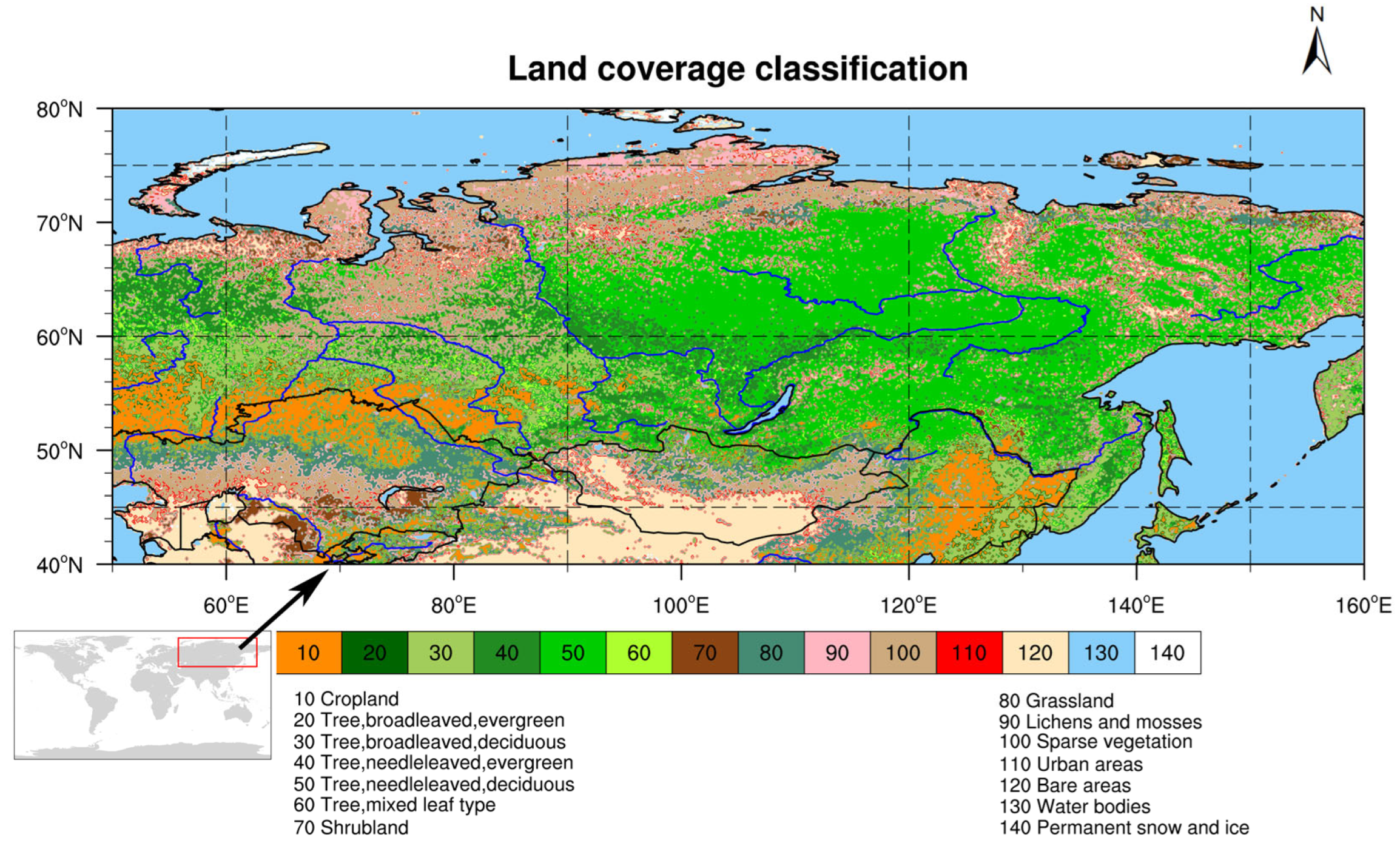
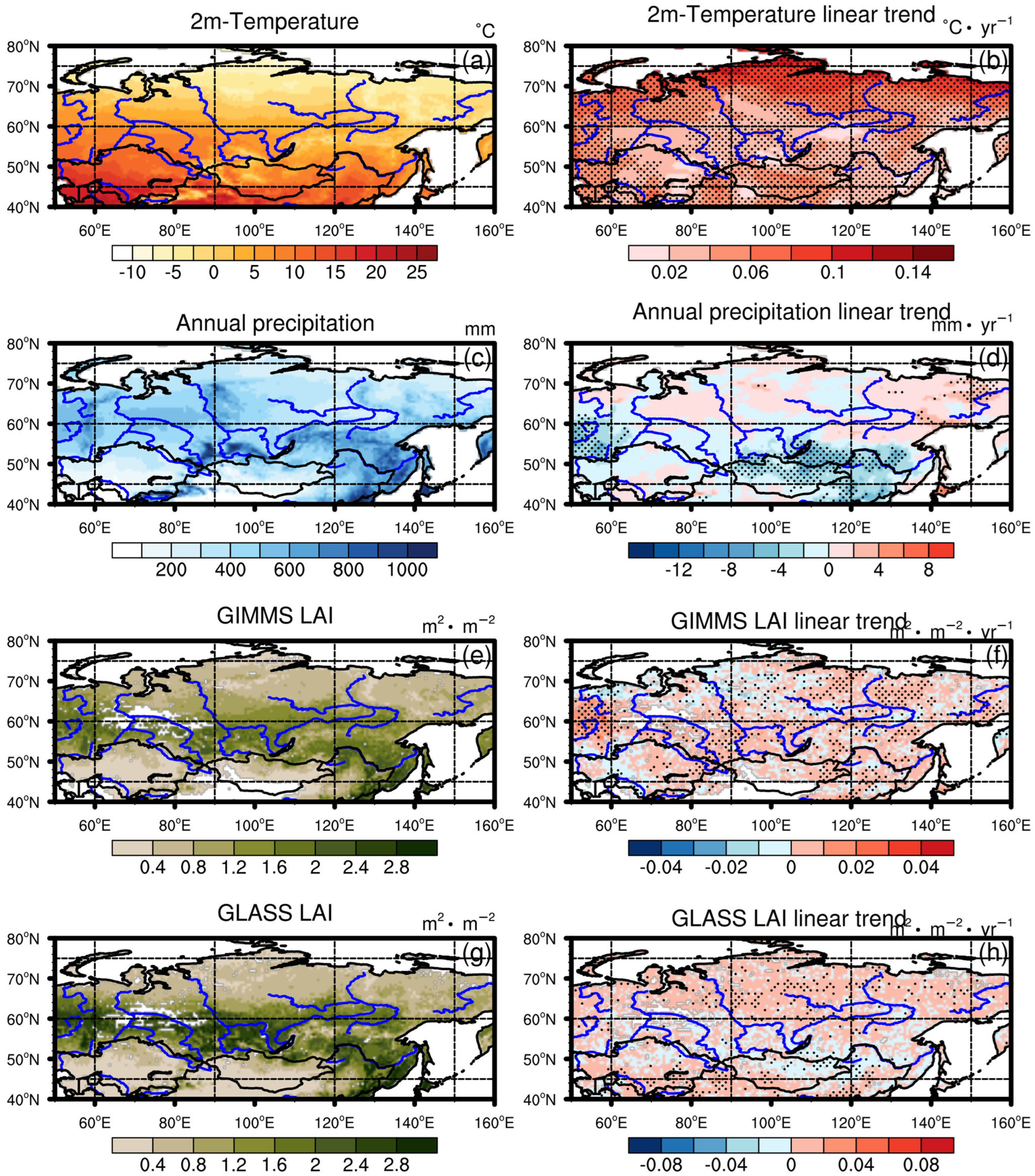
The studied area is located between 50–160 °E and 40–80 °N, which covers most of the high-latitude area in Asia and extends over a land area of approximately 26,624,630 km2. The vegetation types in this area include broadleaf and needleleaf forests, grasses, shrubs, lichens, and mosses (Figure 1). The climate of this area is modulated by monsoons, westerlies, and polar weather systems [47,48]. During 1982–2016, the annual 2 m air temperature ranged from −4 °C to 30 °C, the total precipitation during the growing season from April to November ranged from 200 mm to 1000 mm, and the maximum leaf area index (LAI) was less than 4 (Figure 2). Most of this area experienced significant increases in the 2 m temperature and LAI during the growing season between 1982 and 2016. Pronounced decreases in precipitation were observed in Eastern Europe, the Mongolian Plateau, and north-eastern China.
2.2. Satellite-Based and Climate Datasets
The leaf area index (LAI) is an important biophysical variable of vegetation, which is defined as the one-sided green leaf area per unit of vegetated ground area in broadleaf canopies and as one-half of the total needle surface area per unit of the vegetated ground area in coniferous canopies [49]. It characterizes the physiologically functional surface area through which energy, mass, and momentum are exchanged between the vegetated land surface and the planetary boundary layer [50,51]. It has been widely used for the monitoring and estimating terrestrial vegetation growth, land surface process simulation, and global change studies [52,53,54,55,56,57,58]. To reduce uncertainty and enhance credibility in our analysis of the LAI, we applied two different satellite LAI datasets. One was the Global Inventory Monitoring and Modeling Studies Leaf Area Index third-generation (GIMMS LAI3g) dataset, which is derived from the GIMMS NDVI3g dataset, utilizing an artificial neural network model [51]. It adopts the geographic coordinate system with a 1/12° spatial resolution and semi-monthly temporal frequency, covering the time span from 1982 to 2016. The other was the Global Land Surface Satellite (GLASS) LAI product generated from Advanced Very High-Resolution Radiometer (AVHRR) reflectance data. It has a temporal resolution of eight days at a spatial resolution of 0.05° spanning from 1981 to 2018 [59]. Liang et al. [60] highlighted that these LAI products can reasonably represent the global vegetation characteristics and their seasonal variability with a high reliability and consistency. However, the GLASS LAI products are spatially complete and are attributed to the applied retrieval algorithm, which uses surface reflectance over a one-year period as its input to estimate a one-year LAI profile for each pixel and a series of preprocessing tasks to produce improved algorithm inputs. However, the GIMMS LAI3g (abbreviated as GIMMS LAI) products contain many missing pixels, especially in arctic regions from December to March, which indicates that GIMMS LAI3g data should be preprocessed.
The 2 m temperature and precipitation are derived from the daily agrometeorological EAR5 datasets (AgERA5). This dataset is derived from the hourly European Centre for Medium-Range Weather Forecasts (ECMWF) ERA5 data and presented as the input for agriculture and agro-ecological studies [61]. The annual average of the Climate Data Records Land Cover (CDR-LC) dataset provided by the Copernicus Climate Change Service (C3S) was used in this study to show the present-day vegetation types, as shown in Figure 1. The temporal coverage of land cover dataset is from 1992 to 2020. Except for the shrinking of the Aral Sea caused by human activities, the land cover type changed only a little from 1992 to 2016 in most areas.
These data differ in their spatial resolution, temporal resolution, and data record length (Table 1). To minimize the impact of the differences between different data sources, the AgEAR5 daily 2 m temperature, precipitation, and GLASS LAI were averaged half- monthly to coincide with the time frequency of the GIMMS LAI. For the daily data and semi-monthly data, we divided each month into the first half of the month (16, 15, or 14 days) and the second half of the month (15 or 14 days), and then calculated the average of the half-month data. For GLASS LAI, which had a temporal resolution of 8 days, we first created an empty daily dataset, and then filled it with GLASS LAI data. In other words, the new dataset had the same value for every 8 days. After that, we repeated the above steps, transforming the daily data into semi-monthly data. The LAI and land cover were aggregated every 0.1° to coincide with the spatial scale of the AgEAR5 dataset. Due to the time spans of the datasets used, we selected 1982–2016 as our study period. The growing season from April to November was analyzed in this study.
2.3. Detection of Climate Extremes and Corresponding Vegetation Responses
First, we masked certain poor values to reduce the impact of cloud occlusion on the GIMMS LAI. To ensure that the variables were comparable across seasons and years, we removed the 35 year annual cycle, and then calculated the standardized anomalies of the variables in each grid to remove the annual changes using Equation (1) as follows:
where is the standardized anomaly of the variable in half-month i of year j in each grid. is the multi-year average of the variable in half-month i, and is the multi-year standard deviation. and are derived from the annual-cycle-removed variables.
To analyze the temporal characteristics of climate extremes, such as the year and month in which they occurred, we took the maximum and minimum values of the standardized anomalies throughout the time series for each grid as the research indexes. The maximum or minimum values were found for a specific month of a specific year. To study the spatial characteristics of climate extremes, such as the frequency distribution, we defined the climate extremes as percentiles. Specifically, extremely high value events, such as extreme hot and extreme wet conditions, demonstrate that the variable was greater than the 95th percentile, and extremely low value events, such as extreme cold and extreme dry conditions, demonstrate that the variable is less than the 5th percentile. Compound climate extremes demonstrate both the 2 m temperature and precipitation in extreme situations. Therefore, there are 4 types of compound climate extremes, including extreme hot and wet (the 2 m temperature and precipitation are both greater than the 95th percentile), extreme hot and dry (the 2 m temperature is greater than the 95th percentile and precipitation is less than the 5th percentile), extreme cold and wet (the 2 m temperature is less than the 5th percentile and precipitation is greater than the 95th percentile), and extreme cold and dry climates (the 2 m temperature and precipitation are both less than the 5th percentile), respectively. In addition, the corresponding vegetation responses are also expressed as percentiles in this paper. When an extreme climate occurs, the larger the percentile of LAI is, the more positive the impact of the corresponding extreme climate on it will be. In our study, the spheres with extreme variable states were calculated for each grid and accumulated to evaluate the geographic scope affected.
3. Results
3.1. Extreme States of Vegetation
Before analyzing the impact of extreme 2 m temperatures and precipitation, the extreme values of LAI were investigated to explore the spatial and temporal changes in the extreme vegetation states in the study area.
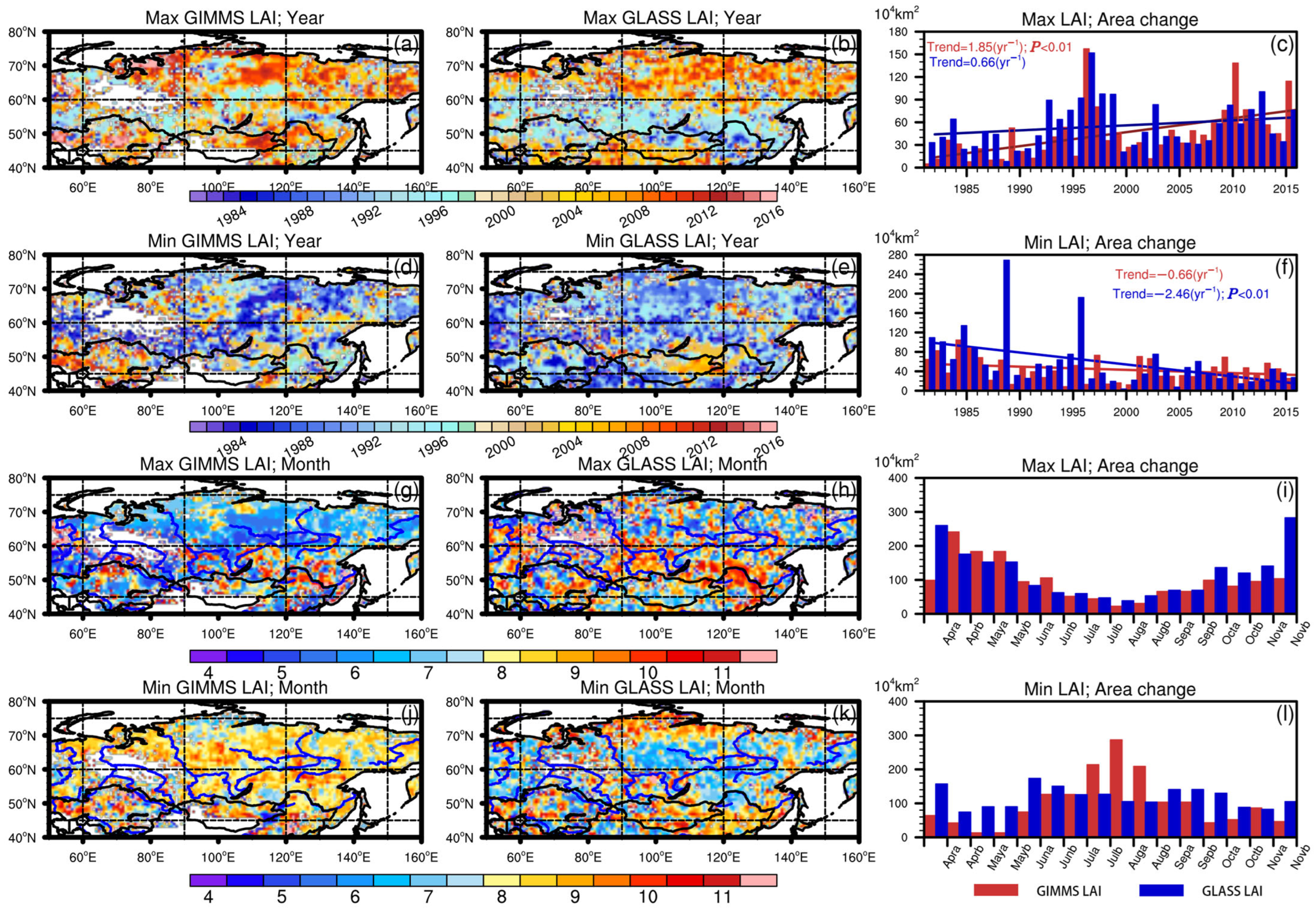
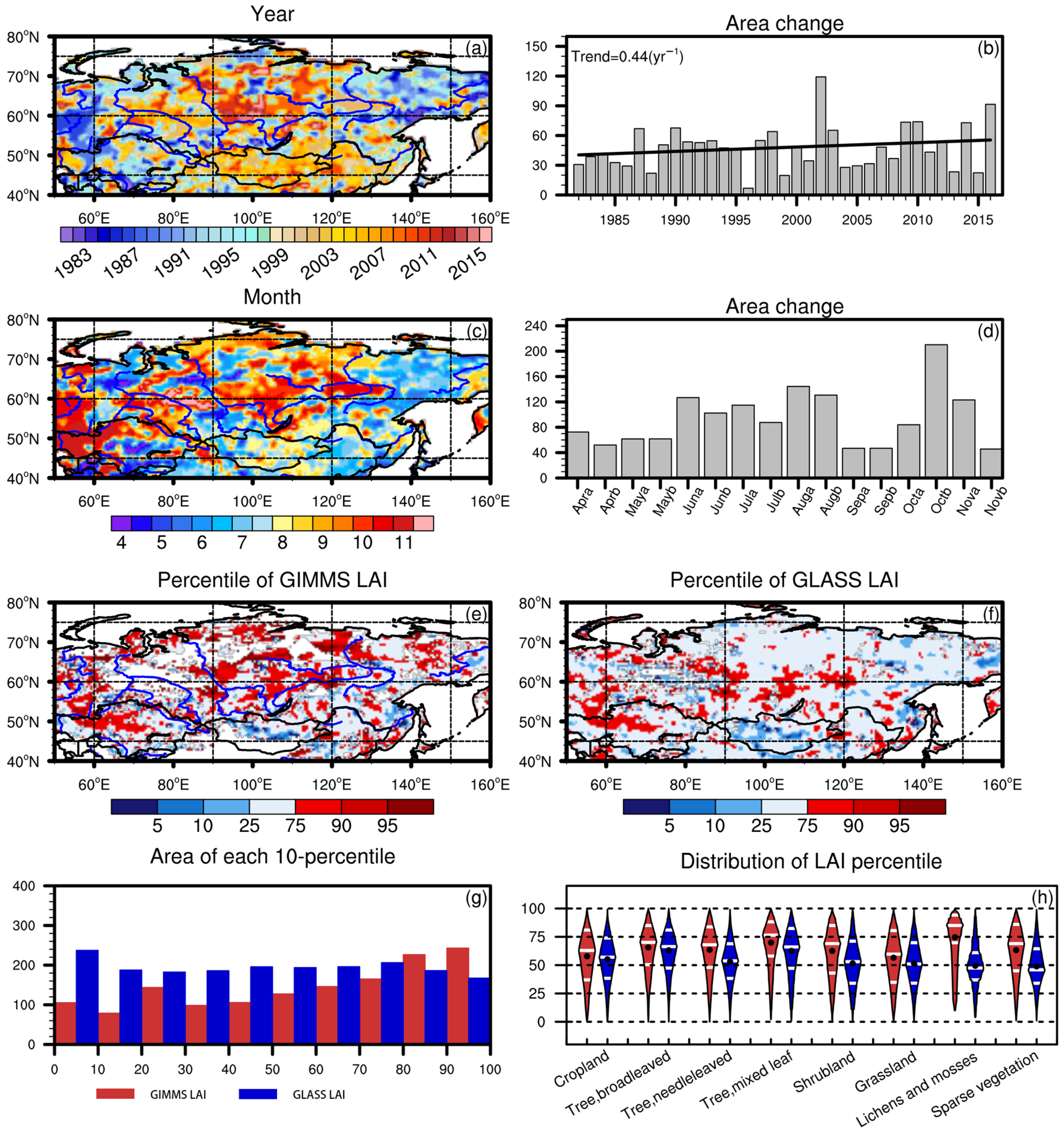
Figure 3a,b shows that the maximum LAI was reached after 2000 in most areas, especially in 2011 and 2016. Additionally, in parts of western and southern Siberia, the GIMMS LAI peaked in 1997. The GLASS LAI peaked in 1997 between 50 °N and 60 °N. The area with the maximum GIMMS LAI and GLASS LAI were found to show increasing trends during 1982–2016 (Figure 3c) at rates of 1.85 × 10⁴ km2/year and 0.66 km2/year, respectively, which was caused by the warming trend and corresponds with the findings of other studies [58,62]. The areas with the minimum GIMMS LAI and GLASS LAI showed decreasing trends at rates of −0.66 km2/year and −2.46 km2/year, respectively (Figure 3f). In the area north of 65 °N, the maximum GIMMS LAI was mostly observed in June and July, and this finding was also revealed by the GLASS LAI. Meanwhile, for the area between 50 °N and 60 °N, the maximum GIMMS LAI was mostly observed in April and May or November, and the maximum GLASS LAI was mostly observed in October and November (Figure 3g,h). The GIMMS LAI in northern Kazakhstan and north-eastern China mostly reached its maximum in autumn. However, most of the area reached the minimum GIMMS LAI in summer between late July and August. The minimum GLASS LAI appeared in June in most of the area. In the areas with sparse vegetation, in which water is the limiting factor for vegetation growth, such as Kazakhstan and north-western China, the minimum GLASS LAI appeared mostly in September (Figure 3j,l). Except for the monthly occurrence of the minimum LAI, the two datasets generally showed similar patterns for the extreme vegetation states.
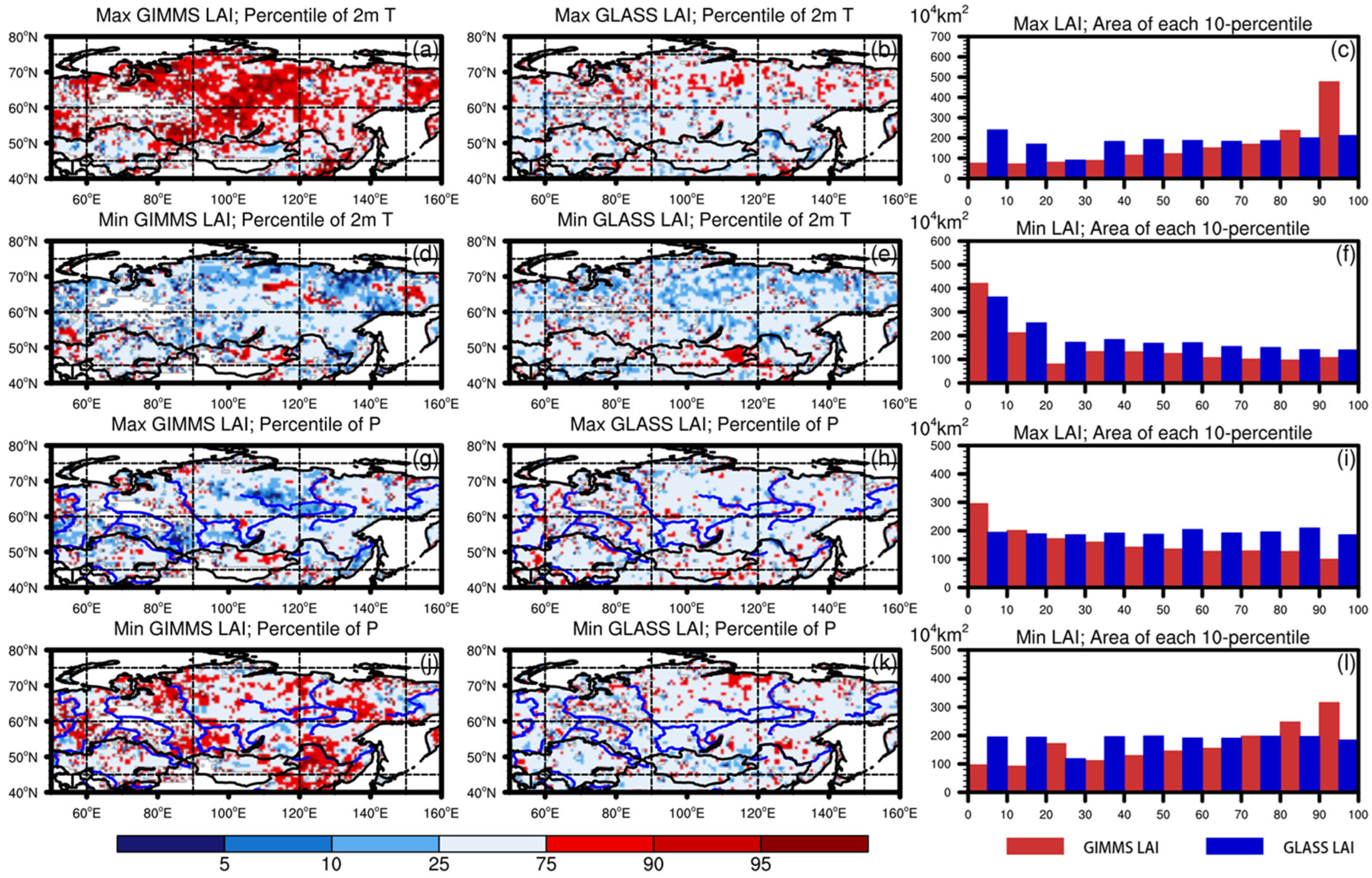
When the GIMMS LAI peaked, nearly half of the area had a 2 m temperature higher than the 80th percentile. Only some arid and semiarid areas, such as Kazakhstan, had a maximum GIMMS LAI accompanied by a lower-than-average temperature (Figure 4a). However, the percentile of the 2 m temperature was fairly well distributed when the GLASS LAI peaked, which suggests that extreme warming had a small impact on the GLASS LAI (Figure 4b). When the GIMMS and GLASS LAI reached their minimum, most of the area had a lower-than-average temperature, with approximately 40% (33%) of the area having a temperature lower than the 20th percentile (Figure 4d–f). However, in some areas of the Mongolian Plateau, the minimum GIMMS LAI and GLASS LAI were accompanied by 2 m temperatures higher than the 75th percentile (Figure 4d,e). Moreover, in Eastern Europe, as well as central and eastern Siberia, the percentile of the 2 m temperature was higher than 75 when the GIMMS LAI reached its minimum (Figure 4d). Nearly 18% of these areas experienced precipitation quantities of lower than the 10th percentile with the maximum GIMMS LAI, while approximately 20% of these areas had precipitation quantities that were higher than the 90th percentile with the minimum GIMMS LAI (Figure 4g,j). The GLASS LAI showed the relatively minimal responses of the vegetation to extreme precipitation compared with that shown by the GIMMS dataset.
3.2. Impact of Temperature Extremes
We then focused on the temporal characteristics of extreme 2 m temperatures or precipitation and explored the synchronous vegetation response. The effects of compound extreme temperatures and precipitation were also explored.
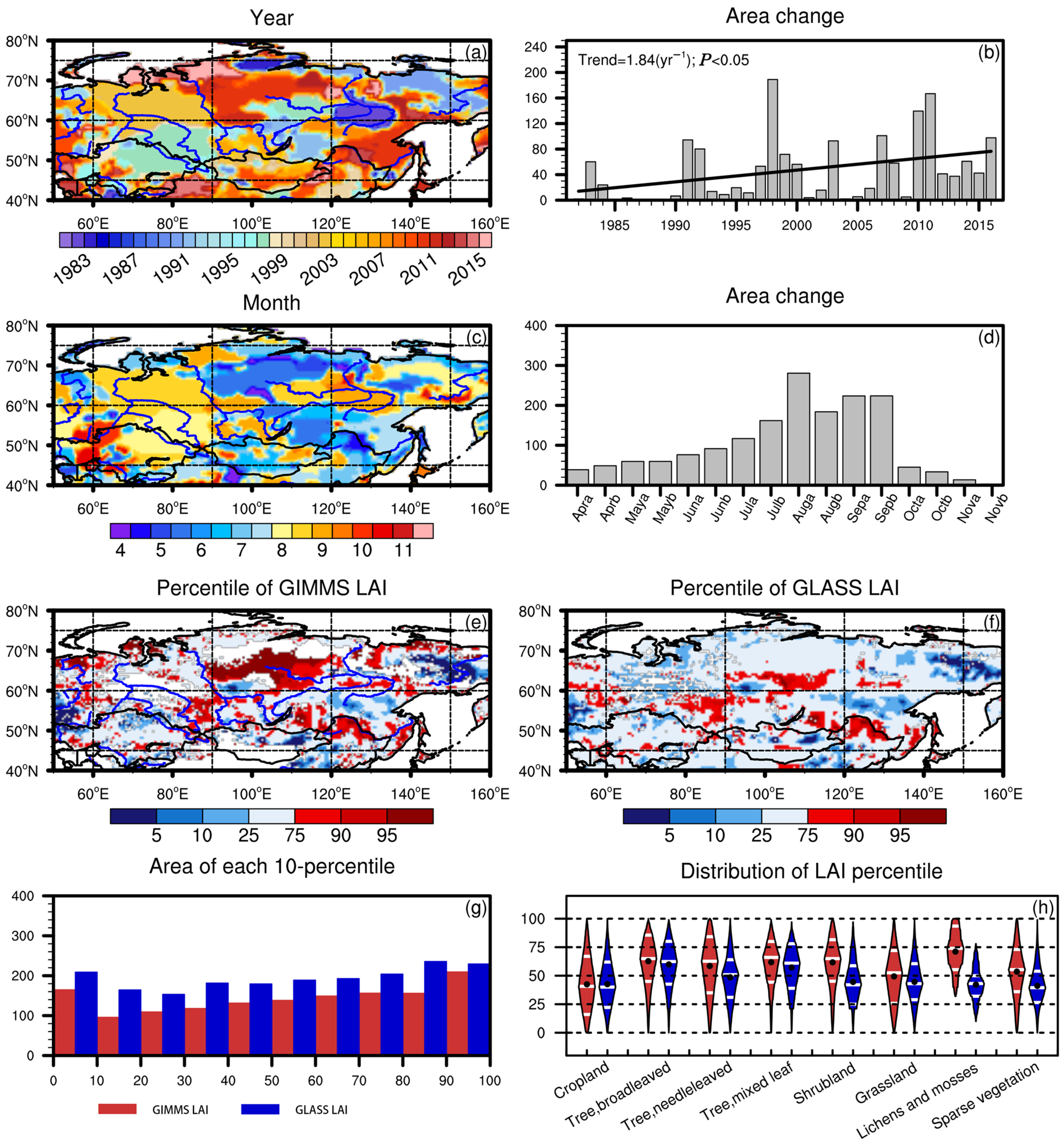
A relatively large area reached the maximum 2 m temperature in the early August of 1998 and late May of 2011 in central Siberia, in the late July of 2011 in the plain south of the Stanovoy Range, and in the August of 2016 on the northern edge of Siberia and some highlands, such as the south-eastern Tibetan Plateau. During these three years, this area accounted for 27% of the total area (Figure 5a–d). In the area, the maximum 2 m temperature was found to increase at a rate of 1.84 × 10⁴ km2/year (), which is consistent with the warming trend from 1982 to 2016. When the maximum 2 m temperature was recorded in central Siberia, south-west Siberia, and north-eastern China, the percentiles of the GIMMS LAI and GLASS LAI were above the 90th percentile, indicating that extremely high temperatures in these areas would greatly promote vegetation growth. However, in Eastern Europe, Kazakhstan, and eastern Siberia, an LAI less than the 10th percentile was observed (Figure 5e,f). Figure 5h shows the probability density distribution of the LAI percentiles for different vegetation types. The two datasets are consistent in that the area covered by trees, including broadleaved, needle-leaved, and mixed leaf trees, shows above-average states, and the area covered by cropland and grassland shows lower-than-average states. However, the two datasets show different responses of shrubs, mosses, and sparse vegetation. The GIMMS LAI basically shows above-average states for the extremely high temperature condition, while the GLASS LAI shows the opposite responses. This implies the inconsistency of the two datasets for vegetation with a small LAI.
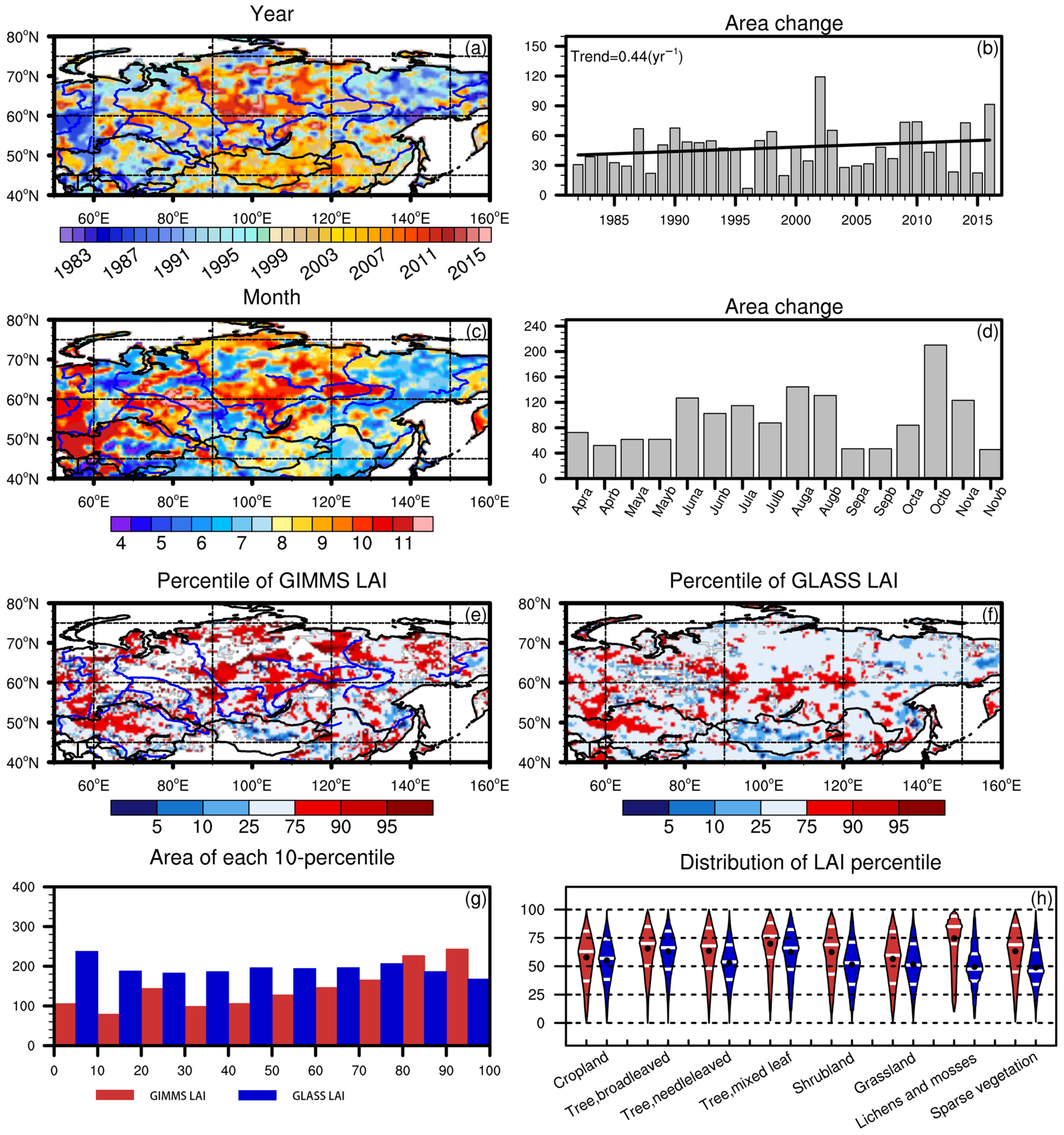
The minimum 2 m temperature was mostly recorded before 2005, accounting for 92% of the total area (Figure 6a). It was mostly recorded at the end of the growing season in October and November, mainly in eastern Kazakhstan, north-eastern China, and Siberia (Figure 6c). Extremely low temperatures were recorded mostly with an LAI of less than the 10th percentile, suggesting that extremely low temperatures generally limit the growth of vegetation in most parts of the area. However, an LAI greater than the 90th percentile was found in the arid and semiarid areas, such as the western parts of Kazakhstan, which are covered by sparse vegetation (Figure 6e–h). Extremely low temperatures generally had a negative effect on vegetation, especially needle-leaved and broadleaved trees. Inconsistent with the GIMMS LAI, the GLASS LAI showed that the growth of shrubs, lichens, mosses, and sparse vegetation was prompted when extreme cold was recorded. This may be related to the quality of the data for the areas covered by these vegetation types (Figure 6h).
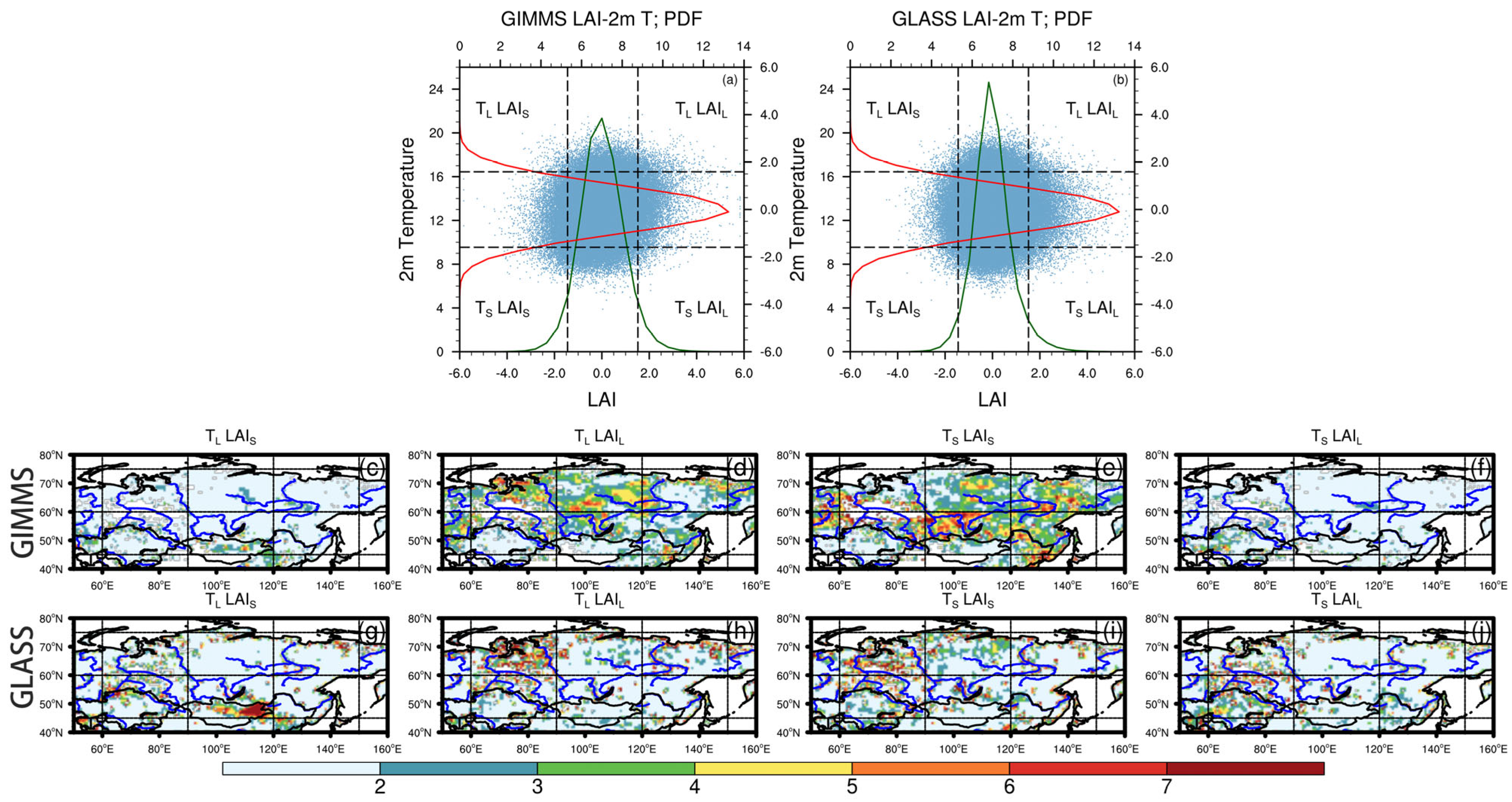
In order to analyze the spatial characteristics of climate extremes and extreme LAI, we further counted the number of times when the four types of extreme temperatures and extreme LAI were recorded simultaneously for each grid (Figure 7). The extremes were specified if the variables were less than the 5th percentile or greater than the 95th percentile; otherwise, they were specified as normal. The four types of extremes were small LAI and cold extremes (TSLAIS), small LAI and warm extremes (TLLAIS), large LAI and cold extremes (TSLAIL), and large LAI and warm extremes (TLLAIL). When the LAI is large, it indicates that the impact of the corresponding climate extremes on it is positive, and the impact is negative when the LAI is small. As shown in Figure 7, TSLAIS were recorded the most frequently, TLLAIL were the second most frequent type, and TLLAIS and TSLAIL were less frequent than the former types. Moreover, the probability distribution of the GLASS LAI was more concentrated than that of the GIMSS LAI, while the GIMMS LAI was better at representing the extreme vegetation states. The GIMMS LAI showed that TSLAIS were recorded mostly between 50 °N and 65 °N in areas where mostly broadleaf trees were distributed (Figure 6h and Figure 7e). TLLAIL were found mostly in Eastern Europe, central Siberia, and some high latitudes at around 60 °N in areas where needleleaf trees are distributed. The GLASS LAI showed similar spatial pattens for the TLLAIL and TSLAIS in western Siberia, but different patterns in areas at approximately 90 °E (Figure 7h,i). This was more apparent in the case of the GIMMS than it was in the case of the GLASS LAI (Figure 7d,e). The distributions of the TLLAIS and TSLAIL shown by the GIMMS LAI and GLASS LAI were similar. Specifically, the TLLAIS were concentrated in the northern Mongolian Plateau, and TSLAIL were seldom recorded in Kazakhstan.
3.3. Impact of Precipitation Extremes
Representing a large number of areas, the maximum precipitation was recorded in the mountains of eastern Siberia in early October 2016, spanning an area of 116 million km2. In addition, the areas with maximum precipitation had a comparatively scattered distribution (Figure 8a–d). Extreme precipitation caused a less-than-the-tenth-percentile GIMMS LAI to be recorded in approximately 20% of the areas. However, a large number of areas in Kazakhstan that are covered by sparse vegetation were found to have GIMMS LAI and GLASS LAI that are greater than the 90th percentile (Figure 8e–h). The average percentiles of all the vegetation types were less than 50%, indicating that extreme precipitation was unfavorable to all the vegetation types. The negative effects were most significant for the trees, whereas they were comparatively small for the crops, grasses, and sparse vegetation (Figure 8h).
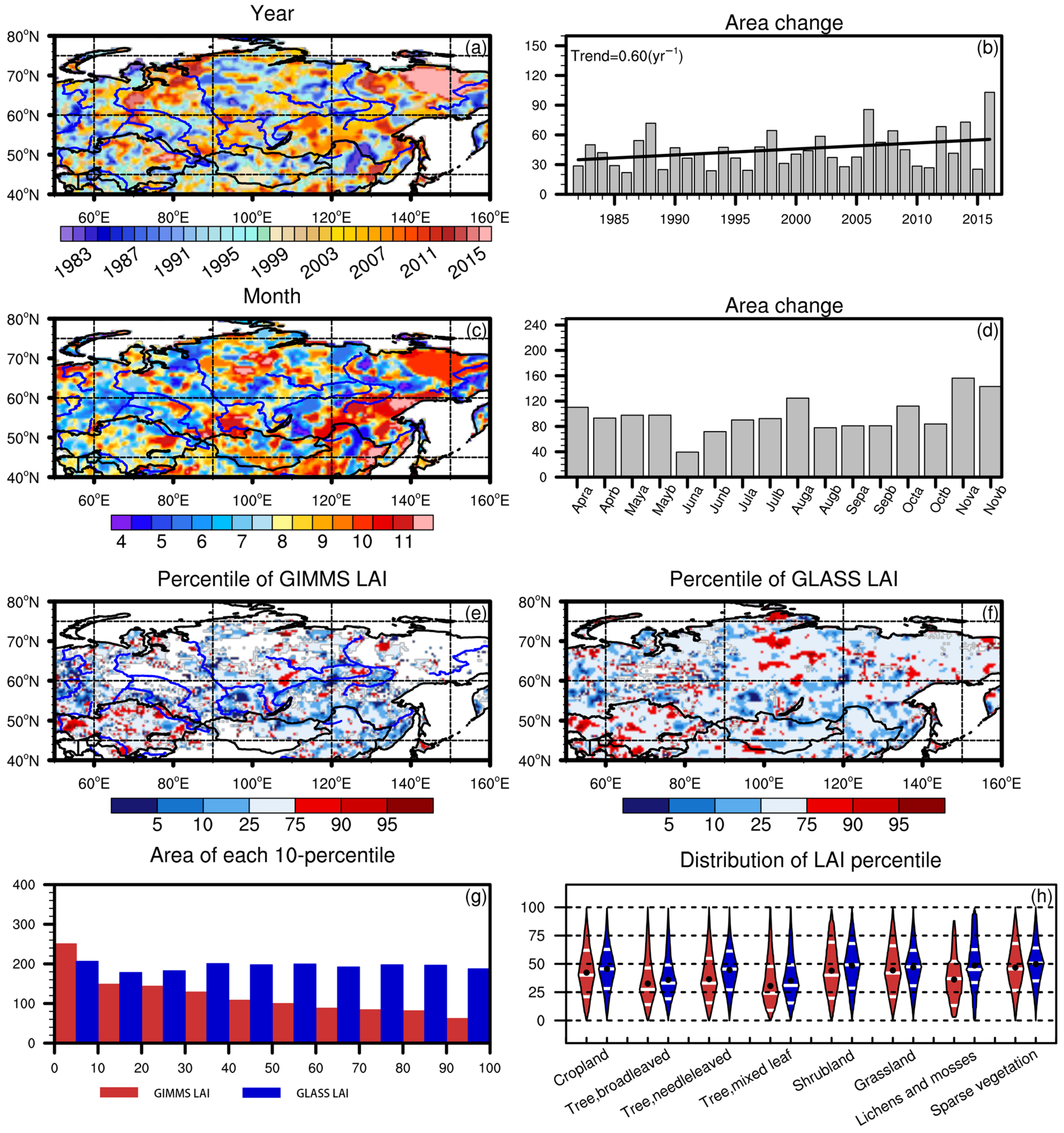
When minimum precipitation recorded, the area with values greater than 90th percentile was the largest (Figure 9g), which suggests that the overall response of vegetation to extreme dryness was positive. Positive impacts of extreme dryness, as shown by the GLASS LAI, were observed in Kazakhstan and central Siberia. The two datasets were consistent regarding the negative responses that were mainly recorded in the transition zone from desert areas to vegetated areas, such as the central Mongolian Plateau. The consistent and positive effects of extreme dry on the trees were clear (Figure 9h). However, the GIMMS LAI implied positive responses of the shrubs, lichens and mosses, and sparse vegetation to extreme dry, while the GLASS LAI showed minimal responses.
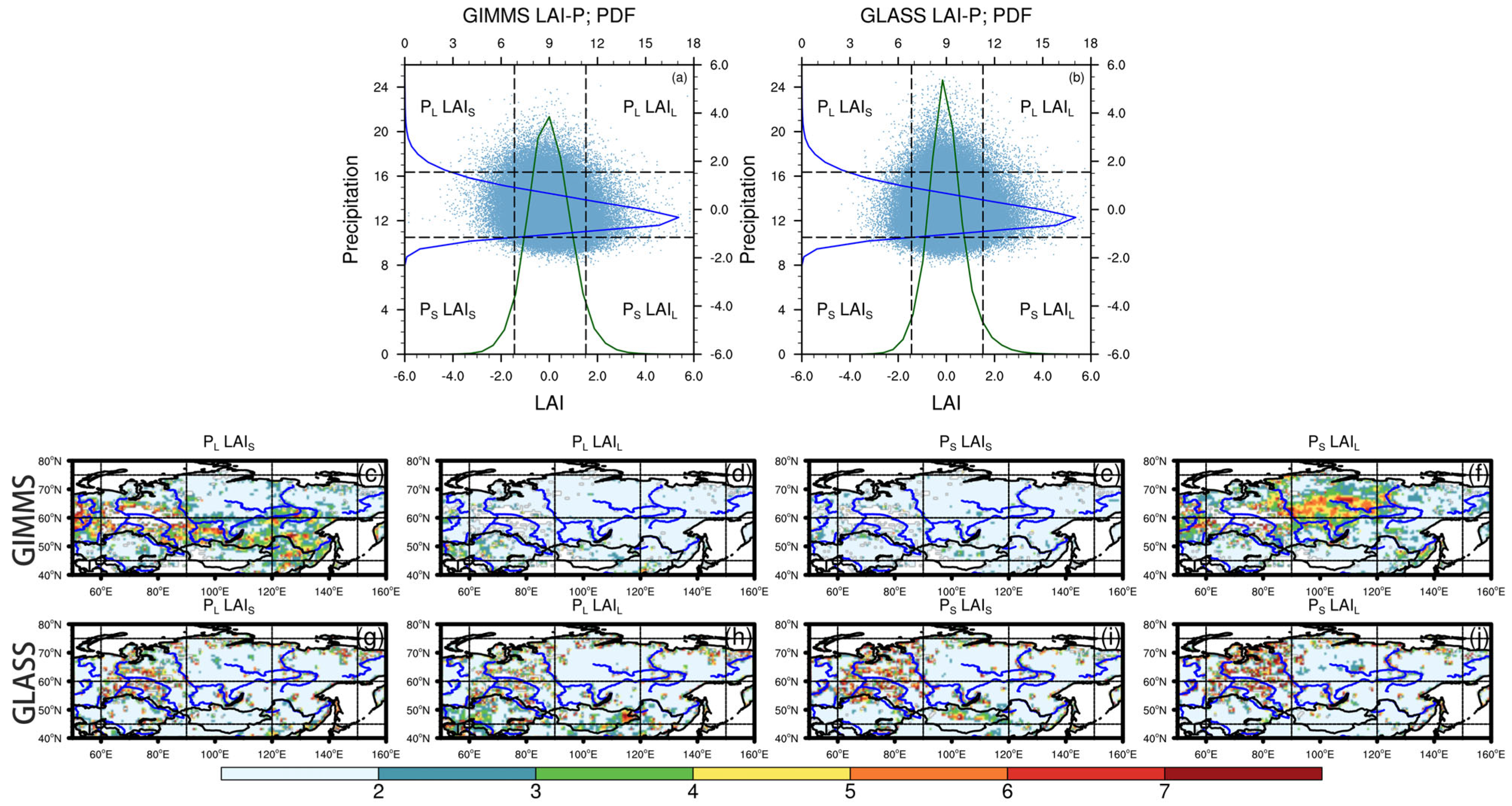
Four types of extreme precipitation vs. extreme LAI, that is, extreme wet/drought and large/small LAI (PLLAIL, PLLAIS, PSLAIL, and PSLAIS), were also observed. The GIMMS data showed that PLLAIS and PSLAIL were recorded more frequently than the other two types were. However, the GLASS data showed approximately equivalent time frequencies for the four types (Figure 10). PLLAIS with GIMMS LAI were mainly recorded between 50 °N and 60 °N, particularly in the southern parts of central Siberia and north-eastern China, where trees occupy the majority of the land area (Figure 10c). PSLAIL with GIMMS LAI were mainly recorded in the Central Siberian Plateau, which is mostly composed of needle-leaved trees and grasslands (Figure 10f). The frequency of PSLAIS with GIMMS LAI was nearly negligible (Figure 10e). The frequency of PLLAIL was also relatively low (Figure 10d,h). However, it was mainly concentrated in Kazakhstan and the Mongolian Plateau, where mostly sparse vegetation is distributed, and it showed a positive response of the vegetation to the extremely wet climate (Figure 10d,e,h,i).
3.4. Impact of Compound Extremes
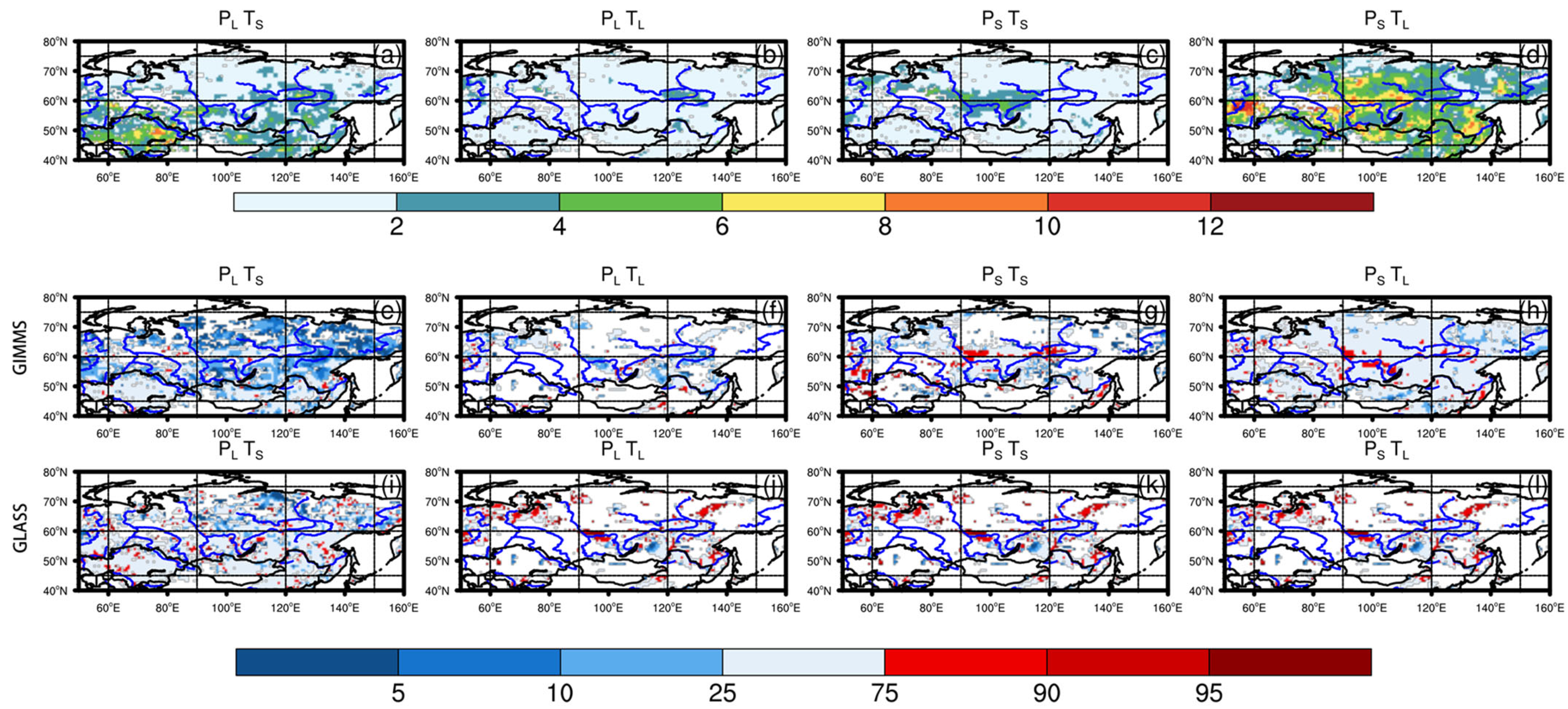
After exploring the effects of extreme temperatures and precipitation on the LAI, we investigated the possible effects of compound extreme temperatures and precipitation. Based on the analysis of the extreme 2 m temperature and precipitation (Figure 11), four types of compound extreme climates were identified. The four types of compound extreme climates were dry and cold (PSTS), wet and hot (PLTL), dry and hot (PSTL), and wet and cold ones (PLTS). We then counted the occurrence of each type in each grid and calculated the corresponding average percentile of the LAI for each type. The most frequent compound extreme climate in this area was PSTL (Figure 11d). It was mainly observed between 50 °N and 60 °N in Asia, central Siberia, and north-eastern China. Basically, the GIMMS and GLASS LAI showed similar responses to the four types of compound extremes. In southern central Siberia, the PSTL climate generally promoted vegetation growth to some extent (Figure 11h,l). The second most frequent compound extreme climate was PLTS (Figure 11a), which mainly appeared in areas south of 60 °N, particularly in Kazakhstan and northern China. It generally benefited vegetation growth in the arid and semi-arid areas. Although they were recorded with limited frequency, the compound PLTS had a detrimental effect on the vegetation at high latitudes (Figure 11e,i). Only some dry areas in Kazakhstan and scattered areas with sparse vegetation were shown to experience a positive effect. The frequency of PSTS and PLTL climates was found to be considerably lower than that of the former two types. PSTS were recorded 2–6 times in 35 years in central Siberia (Figure 11c), and this type was generally accompanied by vegetation prosperity (Figure 11g,k).
4. Discussion
Compared with previous studies that focused on small areas, particularly arid regions, we investigated the responses of vegetation to extreme climates in a relatively large area, namely, the boreal region in Asia, on a semi-monthly basis. We found that extreme hot and/or dry conditions had positive impacts on the forests at high latitudes, which experienced large seasonal variations in temperature and sunlight. The possible mechanisms of this process are that higher temperatures and less rain reflect the conditions of more daylight and less snow cover, resulting in longer growing seasons, more photosynthesis, and greener vegetation [63]. In contrast to global warming and enhanced vegetation cover across the Arctic, extreme cold events can cause negative impacts, including physical and physiological damage, such as premature leaf falling, bending, splitting, breakage, cold injury, and mortality [64,65], in the forests at mid-latitudes [66,67,68,69]. Extremely wet conditions may also inhibit forest growth. The possible reason for this is that water stress in forests is relatively low because the soil in the forest area is able to store a large amount of water. Extreme precipitation leads to wetter conditions, so that the threshold of water available to plants is easily be exceeded, which will have negative effects on forest growth [70]. In arid and semi-arid areas, where mostly sparse vegetation and grass are distributed, such as Kazakhstan and the northern Mongolian Plateau, extremely hot conditions accelerate the evaporation of surface water, resulting in a decrease in soil moisture, which has adverse effects on vegetation growth [71]. However, extremely wet conditions can replenish the soil moisture to some extent, and these events can even infiltrate the deep soil layer, which is beneficial for vegetation [72]. Here, we focused on the synchronous responses of vegetation to climates, without considering the subsequent reactions after the extreme events. Some studies have suggested that cold temperatures during the dormancy period may favor vegetation growth in the following year [73], and grasses can recover soon after a drought event [74]. The possible responses of vegetation after extremes in this area should also be studied in the future.
The relationships of vegetation with extreme climates, observed on a semi-monthly basis, correspond with the findings of previous research, which focused on the relationship between typical vegetation and the climate [57,62,75]. This implies the adaptation of the vegetation in this area. It is projected that this greening trend will continue and expand northward. This has been demonstrated in several numerical studies [39,40,41]. However, prosperous vegetation at high northern latitudes is likely to increase the absorption of solar radiation, further increasing the warming trend. The ways in which this will affect the local and global climates should also be explored.
5. Conclusions
In this study, we investigated the impacts of extreme climates on the vegetation at middle-to-high latitudes in Asia from 1982 to 2016 on a semi-monthly basis. Standardized anomalies, with the annual cycle removed, were scrutinized to determine the extremes of the climate and vegetation states. During these 35 years, the study area experienced both increases and decreases in the frequency of extremely hot and cold conditions. The area with the maximum or minimum LAI increased or decreased during 1982–2016, which corresponds with the global warming trend. The LAI mostly reached its maximum in spring and autumn. Generally, extremely cold conditions accelerated leaf fall during October and November in northern Kazakhstan, southern Siberia, and north-eastern Asia, where forests and croplands occupy the majority of the land area. Extreme heat promoted vegetation growth, particularly during summer in the northern and central parts of Siberia and in north-eastern China, where trees occupied a large proportion of the land. However, a negative effect of extreme heat and a positive effect of extreme cold were also observed, although to a much lesser extent than they were in the former two situations. The negative effect of heat on grass and sparse vegetation was mostly observed in the northern Mongolian Plateau. A positive effect of the cold on mostly sparse vegetation was observed in central Kazakhstan. The impact of extreme precipitation on vegetation was generally negative, with trees at around 50 °N and 60 °N being harmed most frequently. The most frequent response of vegetation to extreme dryness was positive, and it occurred mostly in the cases of mixed trees in central Siberia and lichens and mosses on the northernmost edge of Asia. The positive effect of extreme wetness was found to be much less than those of the former two conditions, and the negative effect of extreme dryness was found to be the least significant one. Extreme precipitation promoted slight vegetation growth in the arid areas in Kazakhstan and the Mongolian Plateau, but it inhibited tree growth in the areas between 50 °N and 60 °N.
The most frequent compound extreme climate of temperature and precipitation was the dry and hot one (PSTL), followed by the wet and cold one (PLTS). Dry and hot (PSTL) climates exist in a vast area that excludes the boreal region, highland areas, and the desert covered by sparse vegetation. Overall, this condition had positive effects, including the promotion of the greening of forests. Wet and cold (PLTS) climates mostly exist south of 60 °N, which includes Kazakhstan, the northern Mongolian Highlands, and northern China. Although it seldom exists at high latitudes, this condition was found to significantly damage boreal vegetation. The dry and cold climate (PSTS) was observed in central Siberia and generally had a positive effect on forest growth. The wet and hot climate (PLTL) was observed as the least frequent condition, and its effect varied with the location.
Generally, the GIMMS and GLASS LAI were consistent regarding the responses of the vegetation to the extremes. Moreover, the GIMMS LAI showed stronger responses of the vegetation than the GLASS LAI did. Extremely cold and/or wet conditions were the most unfavorable conditions for forest growth in the study area. These conditions were recorded more frequently from October to November than they were during the growing season. Dry and/or hot conditions were favorable to boreal forests, particularly during the growing season and before September. The increase in hot areas corresponded to the significant warming trend observed in this area. This observation may suggest that extreme warm conditions promote forest growth. Opposite effects of the extremes were mostly found in arid areas, that is, Kazakhstan and the Mongolia Highlands, primarily occupied by sparse vegetation and grass. This implies the existence of a climate response, specifically, a transition from forest to sparse vegetation in this area.
Author Contributions
Conceptualization, M.Y.; methodology, M.Y., J.W. and Y.W.; software, Y.W.; validation, Y.W.; formal analysis, Y.W.; investigation, Y.W.; resources, Y.W.; data curation, Y.W.; writing—original draft preparation, Y.W.; writing—review and editing, M.Y. and J.W.; visualization, Y.W.; supervision, M.Y. and B.Z.; project administration, M.Y. and B.Z.; funding acquisition, M.Y. and B.Z. All authors have read and agreed to the published version of the manuscript.
Funding
This research was funded by the National Natural Science Foundation of China (grant numbers 41991285 and 42075115).
Data Availability Statement
The 2 m temperature and precipitation data were obtained from the Copernicus Climate Change Service (https://cds.climate.copernicus.eu/cdsapp#!/dataset/sis-agrometeorological-indicators accessed on 13 September 2020). Semi-monthly GIMMS LAI data were obtained from Zhu et al. (https://www.mdpi.com/2072-4292/5/2/927 accessed on 13 September 2020). GLASS LAI data were obtained from Liang et al. (http://www.glass.umd.edu/LAI/AVHRR/, accessed on 28 October 2022).The land cover dataset is also available from the Copernicus Climate Change Service (https://cds.climate.copernicus.eu/cdsapp#!/dataset/satellite-land-cover, accessed on 2 June 2021).
Conflicts of Interest
The authors declare no conflict of interest.
References
- Fang, J.; Zhu, J.; Wang, S.; Yue, C.; Shen, H. Global warming, human-induced carbon emissions, and their uncertainties. Sci. China Earth Sci. 2010, 54, 1458–1468. [Google Scholar] [CrossRef]
- Jia, G.; Shevliakova, E.; Artaxo, P.; De Noblet-Ducoudré, N.; Houghton, R.; House, J.; Kitajima, K.; Lennard, C.; Popp, A.; Sirin, A.; et al. Land—climate interactions. In Climate Change and Land: An IPCC Special Report on Climate Change, Desertification, Land Degradation, Sustainable Land Management, Food Security, and Greenhouse Gas Fluxes in Terrestrial Ecosystems; Shukla, P.R., Skea, J., Calvo Buendia, E., Masson-Delmotte, V., Roberts, D.C., Zhai, P., Slade, R., Connors, S., van Diemen, R., Ferrat, M., Eds.; Cambridge University Press: Cambridge, UK; New York, NY, USA, 2019; Volume 2, pp. 131–248. [Google Scholar]
- Seneviratne, S.I.; Nicholls, N.; Easterling, D.; Goodess, C.M.; Kanae, S.; Kossin, J.; Luo, Y.; Marengo, J.; McInnes, K.; Rahimi, M.; et al. Changes in climate extremes and their impacts on the natural physical environment. In Managing the Risks of Extreme Events and Disasters to Advance Climate Change Adaptation; Field, C.B., Barros, V., Stocker, T.F., Qin, D., Dokken, D.J., Ebi, K.L., Mastrandrea, M.D., Mach, K.J., Plattner, G.K., Al-len, S.K., Eds.; Cambridge University Press: Cambridge, UK; New York, NY, USA, 2012; Volume 3, pp. 109–230. [Google Scholar]
- Seneviratne, S.I.; Donat, M.G.; Pitman, A.J.; Knutti, R.; Wilby, R.L. Allowable CO2 emissions based on regional and impact-related climate targets. Nature 2016, 529, 477–483. [Google Scholar] [CrossRef] [Green Version]
- Sheffield, J.; Wood, E.F.; Roderick, M.L. Little change in global drought over the past 60 years. Nature 2012, 491, 435–438. [Google Scholar] [CrossRef] [PubMed]
- Dai, A. Erratum: Increasing drought under global warming in observations and models. Nat. Clim. Chang. 2013, 3, 171. [Google Scholar] [CrossRef] [Green Version]
- Trenberth, K.E.; Dai, A.; Van Der Schrier, G.; Jones, P.D.; Barichivich, J.; Briffa, K.R.; Sheffield, J. Global warming and changes in drought. Nat. Clim. Chang. 2014, 4, 17–22. [Google Scholar] [CrossRef]
- Mukherjee, S.; Mishra, A.; Trenberth, K.E. Climate Change and Drought: A Perspective on Drought Indices. Curr. Clim. Chang. Rep. 2018, 4, 145–163. [Google Scholar] [CrossRef]
- Spinoni, J.; Barbosa, P.; De Jager, A.; McCormick, N.; Naumann, G.; Vogt, J.V.; Magni, D.; Masante, D.; Mazzeschi, M. A new global database of meteorological drought events from 1951 to 2016. J. Hydrol. Reg. Stud. 2019, 22, 100593. [Google Scholar] [CrossRef] [PubMed]
- Pall, P.; Allen, M.R.; Stone, D.A. Testing the Clausius—Clapeyron constraint on changes in extreme precipitation under CO2 warming. Clim. Dyn. 2007, 28, 351–363. [Google Scholar] [CrossRef]
- Berg, P.M.V.D.; Moseley, C.; Haerter, J.O. Strong increase in convective precipitation in response to higher temperatures. Nat. Geosci. 2013, 6, 181–185. [Google Scholar] [CrossRef]
- Lehmann, J.; Coumou, D.; Frieler, K. Erratum to: Increased record-breaking precipitation events under global warming. Clim. Chang. 2015, 132, 517–518. [Google Scholar] [CrossRef] [Green Version]
- Masson-Delmotte, V.; Zhai, P.; Pirani, A.; Connors, S.L.; Péan, C.; Berger, S.; Caud, N.; Chen, Y.; Goldfarb, L.; Gomis, M.I. (Eds.) IPCC, 2021: Summary for Policymakers. In Climate Change 2021: The Physical Science Basis. Contribution of Working Group I to the Sixth Assessment Report of the Intergovernmental Panel on Climate Change; Cambridge University Press: Cambridge, UK; New York, NY, USA, 2021; pp. 3–32. [Google Scholar]
- Herrera-Estrada, J.E.; Sheffield, J. Uncertainties in Future Projections of Summer Droughts and Heat Waves over the Contiguous United States. J. Clim. 2017, 30, 6225–6246. [Google Scholar] [CrossRef]
- Yu, R.; Zhai, P. Advances in scientific understanding on compound extreme events. Trans. Atmos. Sci. 2021, 44, 645–649. [Google Scholar] [CrossRef]
- Islam, A.R.M.T.; Islam, H.; Shahid, S.; Khatun, M.K.; Ali, M.M.; Rahman, M.; Ibrahim, S.M.; Almoajel, A.M. Spatiotemporal nexus between vegetation change and extreme climatic indices and their possible causes of change. J. Environ. Manag. 2021, 289, 112505. [Google Scholar] [CrossRef] [PubMed]
- Flach, M.; Sippel, S.; Gans, F.; Bastos, A.; Brenning, A.; Reichstein, M.; Mahecha, M.D. Contrasting biosphere responses to hydrometeorological extremes: Revisiting the 2010 western Russian heatwave. Biogeosciences 2018, 15, 6067–6085. [Google Scholar] [CrossRef] [Green Version]
- Cao, M.; Woodward, F.I. Dynamic responses of terrestrial ecosystem carbon cycling to global climate change. Nature 1998, 393, 249–252. [Google Scholar] [CrossRef]
- Seddon, A.W.R.; Macias-Fauria, M.; Long, P.R.; Benz, D.; Willis, K.J. Sensitivity of global terrestrial ecosystems to climate variability. Nature 2016, 531, 229–232. [Google Scholar] [CrossRef] [Green Version]
- Doughty, C.E.; Metcalfe, D.B.; Girardin, C.A.J.; Amézquita, F.F.; Cabrera, D.G.; Huasco, W.H.; Silva-Espejo, J.E.; Araujo-Murakami, A.; da Costa, M.C.; Rocha, W.; et al. Drought impact on forest carbon dynamics and fluxes in Amazonia. Nature 2015, 519, 78–82. [Google Scholar] [CrossRef] [Green Version]
- Baumbach, L.; Siegmund, J.F.; Mittermeier, M.; Donner, R.V. Impacts of temperature extremes on European vegetation during the growing season. Biogeosciences 2017, 14, 4891–4903. [Google Scholar] [CrossRef] [Green Version]
- Wu, X.; Guo, W.; Liu, H.; Li, X.; Peng, C.; Allen, C.D.; Zhang, C.; Wang, P.; Pei, T.; Ma, Y.; et al. Exposures to temperature beyond threshold disproportionately reduce vegetation growth in the northern hemisphere. Natl. Sci. Rev. 2019, 6, 786–795. [Google Scholar] [CrossRef]
- Wen, Y.; Liu, X.; Xin, Q.; Wu, J.; Xu, X.G.; Pei, F.; Li, X.; Du, G.; Cai, Y.; Lin, K.; et al. Cumulative Effects of Climatic Factors on Terrestrial Vegetation Growth. J. Geophys. Res. Biogeosci. 2019, 124, 789–806. [Google Scholar] [CrossRef]
- Karnieli, A.; Agam, N.; Pinker, R.T.; Anderson, M.; Imhoff, M.L.; Gutman, G.G.; Panov, N.; Goldberg, A. Use of NDVI and Land Surface Temperature for Drought Assessment: Merits and Limitations. J. Clim. 2010, 23, 618–633. [Google Scholar] [CrossRef]
- Hao, Y.; Hao, Z.; Fu, Y.; Feng, S.; Zhang, X.; Wu, X.; Hao, F. Probabilistic assessments of the impacts of compound dry and hot events on global vegetation during growing seasons. Environ. Res. Lett. 2021, 16, 074055. [Google Scholar] [CrossRef]
- Dittmar, C.; Fricke, W.; Elling, W. Impact of late frost events on radial growth of common beech (Fagus sylvatica L.) in Southern Germany. Eur. J. For. Res. 2006, 125, 249–259. [Google Scholar] [CrossRef]
- Inouye, D. The ecological and evolutionary significance of frost in the context of climate change. Ecol. Lett. 2000, 3, 457–463. [Google Scholar] [CrossRef]
- Inouye, D.W. Effects of climate change on phenology, frost damage, and floral abundance of montane wildflowers. Ecology 2008, 89, 353–362. [Google Scholar] [CrossRef] [PubMed] [Green Version]
- Hartmann, D.L.; Klein Tank, A.M.G.; Rusticucci, M.; Alexander, L.V.; Brönnimann, S.; Charabi, Y.; Dentener, F.J.; Dlugokencky, E.J.; Easterling, D.R.; Kaplan, A.; et al. Observations: Atmosphere and Surface. In Climate Change 2013: The Physical Science Basis. Contribution of Working Group I to the Fifth Assessment Report of the Intergovernmental Panel on Climate Change; Stocker, T.F., Qin, D., Plattner, G.K., Tignor, M., Allen, S.K., Boschung, J., Nauels, A., Xia, Y., Bex, V., Midgley, P.M., Eds.; Cambridge University Press: Cambridge, UK; New York, NY, USA, 2013; Volume 2, p. 209. [Google Scholar]
- Liu, Q.; Piao, S.; Janssens, I.A.; Fu, Y.; Peng, S.; Lian, X.; Ciais, P.; Myneni, R.B.; Peñuelas, J.; Wang, T. Extension of the growing season increases vegetation exposure to frost. Nat. Commun. 2018, 9, 426. [Google Scholar] [CrossRef] [PubMed] [Green Version]
- Piao, S.; Zhang, X.; Chen, A.; Liu, Q.; Lian, X.; Wang, X.; Peng, S.; Wu, X. The impacts of climate extremes on the terrestrial carbon cycle: A review. Sci. China Earth Sci. 2019, 62, 1551–1563. [Google Scholar] [CrossRef]
- Kundzewicz, Z.; Kanae, S.; Seneviratne, S.; Handmer, J.; Nicholls, N.; Peduzzi, P.; Mechler, R.; Bouwer, L.M.; Arnell, N.; Mach, K.; et al. Flood risk and climate change: Global and regional perspectives. Hydrol. Sci. J. 2014, 59, 1–28. [Google Scholar] [CrossRef] [Green Version]
- Knapp, A.K.; Smith, M.D. Variation Among Biomes in Temporal Dynamics of Aboveground Primary Production. Science 2001, 291, 481–484. [Google Scholar] [CrossRef] [Green Version]
- Jentsch, A.; Kreyling, J.; Elmer, M.; Gellesch, E.; Glaser, B.; Grant, K.; Hein, R.; Lara, M.; Mirzae, H.; Nadler, S.E.; et al. Climate extremes initiate ecosystem-regulating functions while maintaining productivity. J. Ecol. 2011, 99, 689–702. [Google Scholar] [CrossRef]
- Zscheischler, J.; Mahecha, M.; Von Buttlar, J.; Harmeling, S.; Jung, M.; Rammig, A.; Randerson, J.T.; Schölkopf, B.; Seneviratne, S.; Tomelleri, E.; et al. A few extreme events dominate global interannual variability in gross primary production. Environ. Res. Lett. 2014, 9, 035001. [Google Scholar] [CrossRef] [Green Version]
- Xiao, J.; Zhuang, Q.; Liang, E.; Shao, X.; McGuire, A.D.; Moody, A.; Kicklighter, D.W.; Melillo, J.M. Twentieth-Century Droughts and Their Impacts on Terrestrial Carbon Cycling in China. Earth Interact. 2009, 13, 1–31. [Google Scholar] [CrossRef]
- Tuhkanen, S. Climatic parameters and indices in plant geography. In Acta Phytogeographica Suecica; Opulus Press: Uppsala, Sweden, 1980; Volume 67, pp. 1–105. [Google Scholar]
- Hu, X.-M.; Ma, J.-R.; Ying, J.; Cai, M.; Kong, Y.-Q. Inferring future warming in the Arctic from the observed global warming trend and CMIP6 simulations. Adv. Clim. Chang. Res. 2021, 12, 499–507. [Google Scholar] [CrossRef]
- Myneni, R.B.; Keeling, C.D.; Tucker, C.J.; Asrar, G.; Nemani, R.R. Increased plant growth in the northern high latitudes from 1981 to 1991. Nature 1997, 386, 698–702. [Google Scholar] [CrossRef]
- Alo, C.A.; Wang, G. Potential future changes of the terrestrial ecosystem based on climate projections by eight general circulation models. J. Geophys. Res. Biogeosciences 2008, 113, G01004. [Google Scholar] [CrossRef]
- Yu, M.; Wang, G.; Parr, D.; Ahmed, K.F. Future changes of the terrestrial ecosystem based on a dynamic vegetation model driven with RCP8.5 climate projections from 19 GCMs. Clim. Chang. 2014, 127, 257–271. [Google Scholar] [CrossRef]
- Liu, W.; Wang, G.; Yu, M.; Chen, H.; Jiang, Y.; Yang, M.; Shi, Y. Projecting the future vegetation–climate system over East Asia and its RCP-dependence. Clim. Dyn. 2020, 55, 2725–2742. [Google Scholar] [CrossRef]
- Jiang, L.; Guli·jiapaer, G.; Bao, A.; Guo, H.; Ndayisaba, F. Vegetation dynamics and responses to climate change and human activities in Central Asia. Sci. Total. Environ. 2017, 599–600, 967–980. [Google Scholar] [CrossRef]
- Li, C.; Wang, J.; Hu, R.; Yin, S.; Bao, Y.; Ayal, D.Y. Relationship between vegetation change and extreme climate indices on the Inner Mongolia Plateau, China, from 1982 to 2013. Ecol. Indic. 2018, 89, 101–109. [Google Scholar] [CrossRef]
- Dubovyk, O.; Landmann, T.; Dietz, A.; Menz, G. Quantifying the Impacts of Environmental Factors on Vegetation Dynamics over Climatic and Management Gradients of Central Asia. Remote Sens. 2016, 8, 600. [Google Scholar] [CrossRef] [Green Version]
- Luo, M.; Sa, C.; Meng, F.; Duan, Y.; Liu, T.; Bao, Y. Assessing extreme climatic changes on a monthly scale and their implications for vegetation in Central Asia. J. Clean. Prod. 2020, 271, 122396. [Google Scholar] [CrossRef]
- Liu, Y.; Guo, Y. Impact of Pressure System Anomaly over Mid-High Latitude on the Interdecadal Change of East Asia Summer Monsoon. Plateau Meteor. 2005, 24, 129–135. [Google Scholar]
- Yang, S.Y.; Wu, B.Y.; Zhang, R.H.; Zhou, S.W. Propagation of Low-Frequency Oscillation over Eurasian Mid–High Latitude in Winter and Its Association with the Eurasian Teleconnection Pattern. Chin. J. Atmos. Sci. 2013, 38, 121–132. [Google Scholar] [CrossRef]
- Iiames, J.; Cooter, E.; Pilant, A.; Shao, Y. Comparison of EPIC-Simulated and MODIS-Derived Leaf Area Index (LAI) across Multiple Spatial Scales. Remote Sens. 2020, 12, 2764. [Google Scholar] [CrossRef] [PubMed]
- Hu, Y.; Li, H.; Wu, D.; Chen, W.; Zhao, X.; Hou, M.; Li, A.; Zhu, Y. LAI-indicated vegetation dynamic in ecologically fragile region: A case study in the Three-North Shelter Forest program region of China. Ecol. Indic. 2021, 120, 106932. [Google Scholar] [CrossRef]
- Zhu, Z.; Bi, J.; Pan, Y.; Ganguly, S.; Anav, A.; Xu, L.; Samanta, A.; Piao, S.; Nemani, R.R.; Myneni, R.B. Global Data Sets of Vegetation Leaf Area Index (LAI)3g and Fraction of Photosynthetically Active Radiation (FPAR)3g Derived from Global Inventory Modeling and Mapping Studies (GIMMS) Normalized Difference Vegetation Index (NDVI3g) for the Period 1981 to 2011. Remote Sens. 2013, 5, 927–948. [Google Scholar] [CrossRef] [Green Version]
- Semeraro, T.; Mastroleo, G.; Pomes, A.; Luvisi, A.; Gissi, E.; Aretano, R. Modelling fuzzy combination of remote sensing vegetation index for durum wheat crop analysis. Comput. Electron. Agric. 2019, 156, 684–692. [Google Scholar] [CrossRef]
- Seo, H.; Kim, Y. Role of remotely sensed leaf area index assimilation in eco-hydrologic processes in different ecosystems over East Asia with Community Land Model version 4.5—Biogeochemistry. J. Hydrol. 2021, 594, 125957. [Google Scholar] [CrossRef]
- Deng, Y.; Wang, X.; Wang, K.; Ciais, P.; Tang, S.; Jin, L.; Li, L.; Piao, S. Responses of vegetation greenness and carbon cycle to extreme droughts in China. Agric. For. Meteorol. 2021, 298–299, 108307. [Google Scholar] [CrossRef]
- Peano, D.; Materia, S.; Collalti, A.; Alessandri, A.; Anav, A.; Bombelli, A.; Gualdi, S. Global variability of simulated and observed vegetation growing season. J. Geophys. Res. Biogeosci. 2019, 124, 3569–3587. [Google Scholar] [CrossRef] [Green Version]
- Li, Y.; Li, Z.-L.; Wu, H.; Zhou, C.; Liu, X.; Leng, P.; Yang, P.; Wu, W.; Tang, R.; Shang, G.-F.; et al. Biophysical impacts of earth greening can substantially mitigate regional land surface temperature warming. Nat. Commun. 2023, 14, 121. [Google Scholar] [CrossRef]
- Piao, S.; Wang, X.; Park, T.; Chen, C.; Lian, X.; He, Y.; Bjerke, J.W.; Chen, A.; Ciais, P.; Tømmervik, H.; et al. Characteristics, drivers and feedbacks of global greening. Nat. Rev. Earth Environ. 2020, 1, 14–27. [Google Scholar] [CrossRef] [Green Version]
- Chen, J.M.; Ju, W.; Ciais, P.; Viovy, N.; Liu, R.; Liu, Y.; Lu, X. Vegetation structural change since 1981 significantly enhanced the terrestrial carbon sink. Nat. Commun. 2019, 10, 4259. [Google Scholar] [CrossRef] [PubMed] [Green Version]
- Liang, S.; Zhao, X.; Liu, S.; Yuan, W.; Cheng, X.; Xiao, Z.; Zhang, X.; Liu, Q.; Cheng, J.; Tang, H.; et al. A long-term Global LAnd Surface Satellite (GLASS) data-set for environmental studies. Int. J. Digit. Earth 2013, 6, 5–33. [Google Scholar] [CrossRef]
- Xiao, Z.; Liang, S.; Jiang, B. Evaluation of four long time-series global leaf area index products. Agric. For. Meteorol. 2017, 246, 218–230. [Google Scholar] [CrossRef]
- Hersbach, H.; Bell, B.; Berrisford, P.; Hirahara, S.; Horanyi, A.; Muñoz-Sabater, J.; Nicolas, J.; Peubey, C.; Radu, R.; Schepers, D.; et al. The ERA5 global reanalysis. Q. J. R. Meteorol. Soc. 2020, 146, 1999–2049. [Google Scholar] [CrossRef]
- Zhu, Z.; Piao, S.; Myneni, R.B.; Huang, M.; Zeng, Z.; Canadell, J.G.; Ciais, P.; Sitch, S.; Friedlingstein, P.; Arneth, A.; et al. Greening of the Earth and its drivers. Nat. Clim. Chang. 2016, 6, 791–795. [Google Scholar] [CrossRef]
- Quetin, G.R.; Swann, A.L.S. Empirically Derived Sensitivity of Vegetation to Climate across Global Gradients of Temperature and Precipitation. J. Clim. 2017, 30, 5835–5849. [Google Scholar] [CrossRef] [Green Version]
- Zhou, B.; Gu, L.; Ding, Y.; Shao, L.; Wu, Z.; Yang, X.; Li, C.; Li, Z.; Wang, X.; Cao, Y.; et al. The Great 2008 Chinese Ice Storm: Its Socioeconomic–Ecological Impact and Sustainability Lessons Learned. Bull. Am. Meteorol. Soc. 2011, 92, 47–60. [Google Scholar] [CrossRef] [Green Version]
- Wang, X.; Huang, S.; Li, J.; Zhou, G.; Shi, L. Sprouting response of an evergreen broad-leaved forest to a 2008 winter storm in N anling M ountains, southern C hina. Ecosphere 2016, 7, e01395. [Google Scholar] [CrossRef]
- Kim, J.-S.; Kug, J.-S.; Jeong, S.; Yoon, J.-H.; Zeng, N.; Hong, J.; Jeong, J.-H.; Zhao, Y.; Chen, X.; Williams, M.; et al. Arctic warming-induced cold damage to East Asian terrestrial ecosystems. Commun. Earth Environ. 2022, 3, 16. [Google Scholar] [CrossRef]
- Francis, J.A.; Vavrus, S.J. Evidence linking Arctic amplification to extreme weather in mid-latitudes. Geophys. Res. Lett. 2012, 39, L06801. [Google Scholar] [CrossRef]
- Cohen, J.; Screen, J.A.; Furtado, J.C.; Barlow, M.; Whittleston, D.; Coumou, D.; Francis, J.; Dethloff, K.; Entekhabi, D.; Overland, J.; et al. Recent Arctic amplification and extreme mid-latitude weather. Nat. Geosci. 2014, 7, 627–637. [Google Scholar] [CrossRef] [Green Version]
- Kim, J.-S.; Kug, J.-S.; Jeong, S.-J.; Huntzinger, D.N.; Michalak, A.M.; Schwalm, C.R.; Wei, Y.; Schaefer, K. Reduced North American terrestrial primary productivity linked to anomalous Arctic warming. Nat. Geosci. 2017, 10, 572–576. [Google Scholar] [CrossRef]
- Zeppel, M.J.B.; Wilks, J.V.; Lewis, J.D. Impacts of extreme precipitation and seasonal changes in precipitation on plants. Biogeosciences 2014, 11, 3083–3093. [Google Scholar] [CrossRef] [Green Version]
- Wang, S.; Liu, Q.; Huang, C. Vegetation Change and Its Response to Climate Extremes in the Arid Region of Northwest China. Remote Sens. 2021, 13, 1230. [Google Scholar] [CrossRef]
- He, L.; Guo, J.; Yang, W.; Jiang, Q.; Chen, L.; Tang, K. Multifaceted responses of vegetation to average and extreme climate change over global drylands. Sci. Total. Environ. 2023, 858, 159924. [Google Scholar] [CrossRef] [PubMed]
- Lian, X.; Piao, S.; Chen, A.; Wang, K.; Li, X.; Buermann, W.; Huntingford, C.; Peñuelas, J.; Xu, H.; Myneni, R.B. Seasonal biological carryover dominates northern vegetation growth. Nat. Commun. 2021, 12, 983. [Google Scholar] [CrossRef]
- Hossain, L.; Li, J. NDVI-based vegetation dynamics and its resistance and resilience to different intensities of climatic events. Glob. Ecol. Conserv. 2021, 30, e01768. [Google Scholar] [CrossRef]
- Li, G.; Chen, W.; Zhang, X.; Yang, Z.; Wang, Z.; Bi, P. Spatiotemporal changes and driving factors of vegetation in 14 different climatic regions in the global from 1981 to 2018. Environ. Sci. Pollut. Res. 2022, 29, 75322–75337. [Google Scholar] [CrossRef]
Figure 1.
Distribution of vegetation types in 2016. The reclassification is based on the United Nations Food and Agriculture Organization’s (UN FAO) Land Cover Classification System (LCCS).
Figure 1.
Distribution of vegetation types in 2016. The reclassification is based on the United Nations Food and Agriculture Organization’s (UN FAO) Land Cover Classification System (LCCS).

Figure 2.
Averages of 2 m temperature (a), total precipitation (c), GIMMS LAI (e), and GLASS LAI (g) from April to November in 1982–2016 and their linear trends (b,d,f,h). The stippling means the trends are statistically significant at the 5% level based on the two-tailed Student’s t-test.
Figure 2.
Averages of 2 m temperature (a), total precipitation (c), GIMMS LAI (e), and GLASS LAI (g) from April to November in 1982–2016 and their linear trends (b,d,f,h). The stippling means the trends are statistically significant at the 5% level based on the two-tailed Student’s t-test.

Figure 3.
Years (a,b,d,e) and months (g,h,j,k) when the maximum and minimum GIMMS LAI (a,b,g,h) and GLASS LAI (d,e,j,k) were recorded. The histograms in (c,f,i,l) show the area (unit in 104 km2) in which the maximum and minimum values were recorded in different years and half-months. The lines in c and f are the linear trend of change in the area calculated by least-squares regression. The missing values are masked.

Figure 4.
Percentiles of the 2 m air temperature (a,b,d,e) and precipitation (g,h,j,k) when the maximum (a,b,g,h) and minimum (d,e,j,k) GIMMS LAI (a,b,g,h) and GLASS LAI (d,e,j,k) were recorded. The histograms in (c,f,i,l) show the corresponding percentile distributions of the accumulated area (unit in 104 km2).

Figure 5.
Years (a), half-months (c), and percentiles of GIMMS LAI (e) and GLASS LAI (f) when the maximum 2 m temperature was recorded, and the corresponding accumulated areas (unit in 104 km2 (b,d,g)). The box plot (h) shows the percentile of the LAI for different vegetation types, with the white lines showing the 25th, 50th, and 75th percentiles, and the dots showing the averages. The line in b is the linear trend calculated by least-squares regression.

Figure 6.
Same as Figure 5 but for the LAI when the minimum 2 m temperature was recorded. Years (a), half-months (c), and percentiles of GIMMS LAI (e) and GLASS LAI (f) when the minimum 2 m temperature was recorded, and the corresponding accumulated areas (unit in 104 km2 (b,d,g)). The box plot (h) shows the percentile of the LAI for different vegetation types, with the white lines showing the 25th, 50th, and 75th percentiles, and the dots showing the averages. The line in b is the linear trend calculated by least-squares regression.

Figure 7.
(a,b) Scatter plot of the 2 m temperature and LAI with their probability distributions overlaid (lines). The black dashed lines mark the of 5th and 95th percentiles. The subscripts “L” and “S” represent values of the variables larger than the 95th percentile and smaller than 5th percentile, respectively. (c–j) Frequencies of the 4-compound extreme LAI vs. extreme temperature situations (GIMMS LAI: (a,c–f); GLASS LAI: (b,g–j)).

Figure 8.
Same as Figure 5, but for the LAI when the maximum precipitation was recorded. Years (a), half-months (c), and percentiles of GIMMS LAI (e) and GLASS LAI (f) when the maximum precipitation was recorded, and the corresponding accumulated areas (unit in 104 km2. (b,d,g). The box plot (h) shows the percentile of the LAI for different vegetation types, with the white lines showing the 25th, 50th, and 75th percentiles, and the dots showing the averages. The line in b is the linear trend calculated by least-squares regression.

Figure 9.
Same as Figure 5, but for the LAI when the minimum precipitation was recorded. Years (a), half-months (c), and percentiles of GIMMS LAI (e) and GLASS LAI (f) when the minimum precipitation was recorded, and the corresponding accumulated areas (unit in 104 km2. (b,d,g). The box plot (h) shows the percentile of the LAI for different vegetation types, with the white lines showing the 25th, 50th, and 75th percentiles, and the dots showing the averages. The line in b is the linear trend calculated by least-squares regression.

Figure 10.
Same as Figure 7, but for the precipitation–LAI relationship. (a,b) Scatter plot of the precipitation and LAI with their probability distributions overlaid (lines). The black dashed lines mark the of 5th and 95th percentiles. The subscripts “L” and “S” represent values of the variables larger than the 95th percentile and smaller than 5th percentile, respectively. (c–j) Frequencies of the 4-compound extreme LAI vs. extreme precipitation situations (GIMMS LAI: (a,c–f); GLASS LAI: (b,g–j)).

Figure 11.
Frequencies of the four types of compound extreme precipitation and temperature climates (a–d) and the corresponding average percentiles of the GIMMS LAI (e–h) and GLASS LAI (i–l).
Figure 11.
Frequencies of the four types of compound extreme precipitation and temperature climates (a–d) and the corresponding average percentiles of the GIMMS LAI (e–h) and GLASS LAI (i–l).


Table 1.
Data used in this study.
| Dataset | Type | Variables | Resolution | Frequency | Record Length | Missing Value of the Land |
|---|---|---|---|---|---|---|
| AgERA5 | Reanalysis | Temperature, precipitation | 0.1° × 0.1° | Daily | 1979–present | No |
| GIMMS | Satellite | LAI | 1/12° × 1/12° | Semi-monthly | 1982–2016 | Yes |
| GLASS | Satellite | LAI | 0.05° × 0.05° | 8 d | 1981–2018 | No |
| C3S | Satellite | Land cover class | 300 m × 300 m | Yearly | 1992–2020 | No |
Disclaimer/Publisher’s Note: The statements, opinions and data contained in all publications are solely those of the individual author(s) and contributor(s) and not of MDPI and/or the editor(s). MDPI and/or the editor(s) disclaim responsibility for any injury to people or property resulting from any ideas, methods, instructions or products referred to in the content. |
© 2023 by the authors. Licensee MDPI, Basel, Switzerland. This article is an open access article distributed under the terms and conditions of the Creative Commons Attribution (CC BY) license (https://creativecommons.org/licenses/by/4.0/).
Share and Cite
MDPI and ACS Style
Wei, Y.; Yu, M.; Wei, J.; Zhou, B. Impacts of Extreme Climates on Vegetation at Middle-to-High Latitudes in Asia. Remote Sens. 2023, 15, 1251. https://doi.org/10.3390/rs15051251
AMA Style
Wei Y, Yu M, Wei J, Zhou B. Impacts of Extreme Climates on Vegetation at Middle-to-High Latitudes in Asia. Remote Sensing. 2023; 15(5):1251. https://doi.org/10.3390/rs15051251
Chicago/Turabian StyleWei, Yuchen, Miao Yu, Jiangfeng Wei, and Botao Zhou. 2023. "Impacts of Extreme Climates on Vegetation at Middle-to-High Latitudes in Asia" Remote Sensing 15, no. 5: 1251. https://doi.org/10.3390/rs15051251
Note that from the first issue of 2016, this journal uses article numbers instead of page numbers. See further details here.