
Semantic Segmentation of Remote Sensing Imagery Based on Multiscale Deformable CNN and DenseCRF


1
Department of Space Microwave Remote Sensing System, Aerospace Information Research Institute, Chinese Academy of Sciences, Beijing 100190, China
2
School of Electronic, Electrical and Communication Engineering, University of Chinese Academy of Sciences, Beijing 100039, China
*
Author to whom correspondence should be addressed.
Remote Sens. 2023, 15(5), 1229; https://doi.org/10.3390/rs15051229
Submission received: 18 January 2023
/
Revised: 21 February 2023
/
Accepted: 21 February 2023
/
Published: 23 February 2023
(This article belongs to the Section AI Remote Sensing)
Abstract
:The semantic segmentation of remote sensing images is a significant research direction in digital image processing. The complex background environment, irregular size and shape of objects, and similar appearance of different categories of remote sensing images have brought great challenges to remote sensing image segmentation tasks. Traditional convolutional-neural-network-based models often ignore spatial information in the feature extraction stage and pay less attention to global context information. However, spatial context information is important in complex remote sensing images, which means that the segmentation effect of traditional models needs to be improved. In addition, neural networks with a superior segmentation performance often suffer from the problem of high computational resource consumption. To address the above issues, this paper proposes a combination model of a modified multiscale deformable convolutional neural network (mmsDCNN) and dense conditional random field (DenseCRF). Firstly, we designed a lightweight multiscale deformable convolutional network (mmsDCNN) with a large receptive field to generate a preliminary prediction probability map at each pixel. The output of the mmsDCNN model is a coarse segmentation result map, which has the same size as the input image. In addition, the preliminary segmentation result map contains rich multiscale features. Then, the multi-level DenseCRF model based on the superpixel level and the pixel level is proposed, which can make full use of the context information of the image at different levels and further optimize the rough segmentation result of mmsDCNN. To be specific, we converted the pixel-level preliminary probability map into a superpixel-level predicted probability map according to the simple linear iterative clustering (SILC) algorithm and defined the potential function of the DenseCRF model based on this. Furthermore, we added the pixel-level potential function constraint term to the superpixel-based Gaussian potential function to obtain a combined Gaussian potential function, which enabled our model to consider the features of various scales and prevent poor superpixel segmentation results from affecting the final result. To restore the contour of the object more clearly, we utilized the Sketch token edge detection algorithm to extract the edge contour features of the image and fused them into the potential function of the DenseCRF model. Finally, extensive experiments on the Potsdam and Vaihingen datasets demonstrated that the proposed model exhibited significant advantages compared to the current state-of-the-art models.
1. Introduction
At present, image semantic segmentation (ISS) is one of the most-significant areas of research in the field of digital image processing and computer vision. Compared with traditional image segmentation, ISS adds semantic information to the target and foreground of the image on this basis and can obtain the information that the image itself needs to express according to the texture, color, and other high-level semantic features of the image, which is more practical [1]. The difference between remote sensing image semantic segmentation and ordinary image semantic segmentation lies in the different processing objects. Specifically, the semantic segmentation of remote sensing images refers to the analysis of the spectrum, color, shape, and spatial information of various ground objects in remote sensing images, divides the feature space into independent subspaces, and finally, assigns each pixel in the image predetermined semantic tags. Remote sensing images contain richer ground object information and vary in size, color, and orientation, which leads to the emergence of inter-class similarities and intra-class variability [2,3,4]. For instance, “stadium”, “church”, and “baseballfield” may appear in “school”, and there may be large differences in different “school” scenes, as shown in Figure 1. Moreover, remote sensing images often have a complex background environment, irregular object shapes, similar appearances in different categories, and other factors that are not conducive to image segmentation. In particular, compared with natural images that only contain the three channels of RGB, high-resolution multispectral remote sensing images contain more channels, which contain richer ground features and a more complex spatial distribution. On account of the above-mentioned factors, the task of the semantic segmentation of remote sensing images is far more complicated than that of natural images. Furthermore, many natural image semantic segmentation models do not perform satisfactorily on remote sensing images. Recently, there has been increasing research on the semantic segmentation of remote sensing images. However, due to the above problems, the semantic segmentation of remote sensing images is still worth further study [5,6,7,8].
Currently, several new segmentation tasks have emerged, including instance segmentation and panoptic segmentation [9,10]. Different from basic semantic segmentation, instance segmentation needs to label different individual aspects of the same object [11,12,13]. On the basis of instance segmentation, panoptic segmentation needs to detect and segment all objects in the image, including the background [14,15,16]. It can be found that the instance segmentation and panoptic segmentation tasks are more complicated. At present, there are still many problems in the research of instance segmentation and panoptic segmentation, such as object occlusion and image degradation [10,11]. Although there are many new research branches of semantic segmentation, this does not mean that the basic semantic segmentation research is worthless. The semantic segmentation of remote sensing images plays an important role in many applications such as resource surveys, disaster detection, and urban planning [17]. However, due to the complexity of remote sensing images, there are many problems to be solved in basic semantic segmentation. For example, how to improve the accuracy and execution speed of remote sensing image semantic segmentation is still a problem worth studying. When the performance of the basic remote sensing semantic segmentation model is satisfactory, it is reasonable to further consider the instance segmentation and panoptic segmentation of remote sensing images.
The results of remote sensing image segmentation are mainly determined by multiscale feature extraction, spatial context information, and boundary information [18]. First of all, rich features are conducive to determining the object categories in images in complex environments. In particular, feature extraction at different scales can effectively alleviate the segmentation impact caused by the differences between object sizes in the image. Second, the global spatial context information can help determine the category of adjacent pixels, because it is not easy to obtain satisfactory segmentation results using only local information. Finally, since the satellite is not stationary when taking remote sensing images, the boundaries of objects in the image are often unclear, so more attention should be paid to the edge details of objects during image segmentation.
Traditional remote sensing image segmentation models generally use manual feature extractors for feature extraction and then use traditional machine learning classification models for the final pixel classification operations. Traditional feature extraction models include oriented FAST and rotated brief (ORB) [19], local binary pattern (LBP) [20], speeded up robust features (SURF) [21], etc. Traditional classification methods consist of support vector machine [22], logistic regression [23], etc. However, due to the complex background environment in remote sensing images, the performance of traditional remote sensing image segmentation models is often unsatisfactory. Additionally, the abilities of traditional feature extraction models cannot meet the needs of practical applications.
Deep learning has been widely used in image recognition [24,25], image classification [26,27], video prediction [28,29], and other fields. In particular, deep convolutional neural networks (DCNNs) with strong feature extraction capabilities are popular in computer vision [30,31,32,33,34,35,36,37]. For instance, Reference [38] designed a YOLOv3 model with four scale detection layers for pavement crack detection, using a multiscale fusion structure and an efficient cross-linking (EIoU) loss function. Recently, DCNNs have been gradually used in image semantic segmentation tasks. For example, Reference [39] built a segmentation model called U-Net, which fuses the features of different scales to obtain segmentation results. However, the U-net model does not consider the spatial context information in the image. The PSPNet [40] model obtains contextual information through a pyramid pooling module, which improves the segmentation performance. However, it has high computational complexity and poor efficiency. Reference [41] designed a high-resolution network (HRNet), which fuses structural features and high-level semantic information at the output end, improving the spatial information extraction ability of images, but ignoring local information. For the problem of HRNet, Reference [42] used the attention mechanism to improve the recognition performance of the model for local regions. However, this model is very resource-intensive and has a large amount of redundant information. Additionally, Reference [18] proposed a high-resolution context extraction network (HRCNet) based on a high-resolution network for the semantic segmentation of remote sensing images. Reference [43] built a multi-attention network (MANet) to extract contextual dependencies in images through multiple efficient attention modules. However, the multiscale context fusion effect of HRCNet and MANet needs to be improved, and both have the problem of high computational complexity. In summary, during the semantic segmentation task of remote sensing images in complex environments, the current CNN-based model does not pay enough attention to global context information, and its performance is not completely convincing [44]. In addition, networks with a superior segmentation performance often have the problem of excessive computing resource consumption.
Considering the main factors affecting the semantic segmentation of remote sensing images and the problems of deep learning models in the semantic segmentation of remote sensing images, this paper proposes the mmsDCNN-DenseCRF model, in which a modified multiscale deformable convolutional neural network (mmsDCNN) is used for multiscale feature extraction, while DenseCRF is utilized to capture semantic information and global context dependency and optimize rough segmentation results such as edge refinement. First, a lightweight multiscale deformable convolution neural network is proposed, which is based on the modified multiscale convolutional neural network (mmsCNN) designed in our previous work [45]. The mmsDCNN model adds an offset to the sampling position of mmsCNN convolution, allowing for the convolutional kernel to adaptively choose the receptive field size with only a slight increase in computing resources. In addition, the mmsDCNN can achieve a balance between strong multiscale feature extraction performance and low computational complexity. We used the mmsDCNN to extract rich multiscale features and obtain preliminary prediction results. Subsequently, a multi-level DenseCRF based on the superpixel and pixel level is proposed as a back-end optimization module, which can make full use of spatial context information at different granularities. The multi-level DenseCRF model considers the relationship between each pixel and all other pixels, establishes a dependency between all pixel pairs in the image, and uses the interdependencies between pixels to introduce the global information of the image, which is suitable for the semantic segmentation task of remote sensing images in complex environments [46]. Although DenseCRF improves the robustness of processing images with semantic segmentation, it can only determine the region position and approximate shape contour of the object of interest in the image marking results. As a result, the real boundary of the segmented region cannot be accurately obtained, since there are still fuzzy edge categories or segmentation mistakes. To solve the above problems, we used the Sketch token edge detection algorithm [47] to extract the edge contour features of the image and fuse the edge contour features into the potential function of the DenseCRF model. In summary, this paper proposes a new idea and specific implementation for the problems existing in the existing models based on convolutional neural networks in remote sensing image segmentation tasks.
The main contributions are as follows:
- A framework of the mmsDCNN-DenseCRF combined model for the semantic segmentation of remote sensing images is proposed.
- We designed a lightweight mmsDCNN model, which incorporates deformable convolution into the mmsCNN proposed in our previous work [45]. Notably, the mmsDCNN adds an offset to the sampling position of the mmsCNN convolution, which enables the convolutional kernel to adaptively determine the receptive field size. Compared with the mmsCNN, the mmsDCNN can achieve a satisfactory performance improvement with only a tiny increase in the computational complexity.
- The multi-level DenseCRF model based on the superpixel level and pixel level is proposed. We combined the pixel-level potential function with the superpixel-based potential function to obtain the final Gaussian potential function, which enables our model to consider features of various scales and the context information of the image and prevents poor superpixel segmentation results from affecting the final result.
- To solve the problem of blurring edge categories or segmentation errors in the semantic segmentation task of DenseCRF, we utilized a Sketch token edge detection algorithm to extract the edge contour features of the image and integrated them into the Gaussian potential function of the DenseCRF model.
The remainder of the article is organized as follows. Section 2 introduces the modified multiscale deformable convolutional neural network (mmsDCNN), and the multi-level DenseCRF model. In Section 3, we conduct some comparative experiments on the public dataset, i.e., the International Society for Photogrammetry and Remote Sensing (ISPRS) [48]. Finally, Section 5 provides a summary of the article.
2. Methodology
The pipeline of the proposed model is shown in Figure 2. The following two parts are included: the modified multiscale deformable convolutional neural network (mmsDCNN) and the multi-level DenseCRF model.
2.1. mmsDCNN
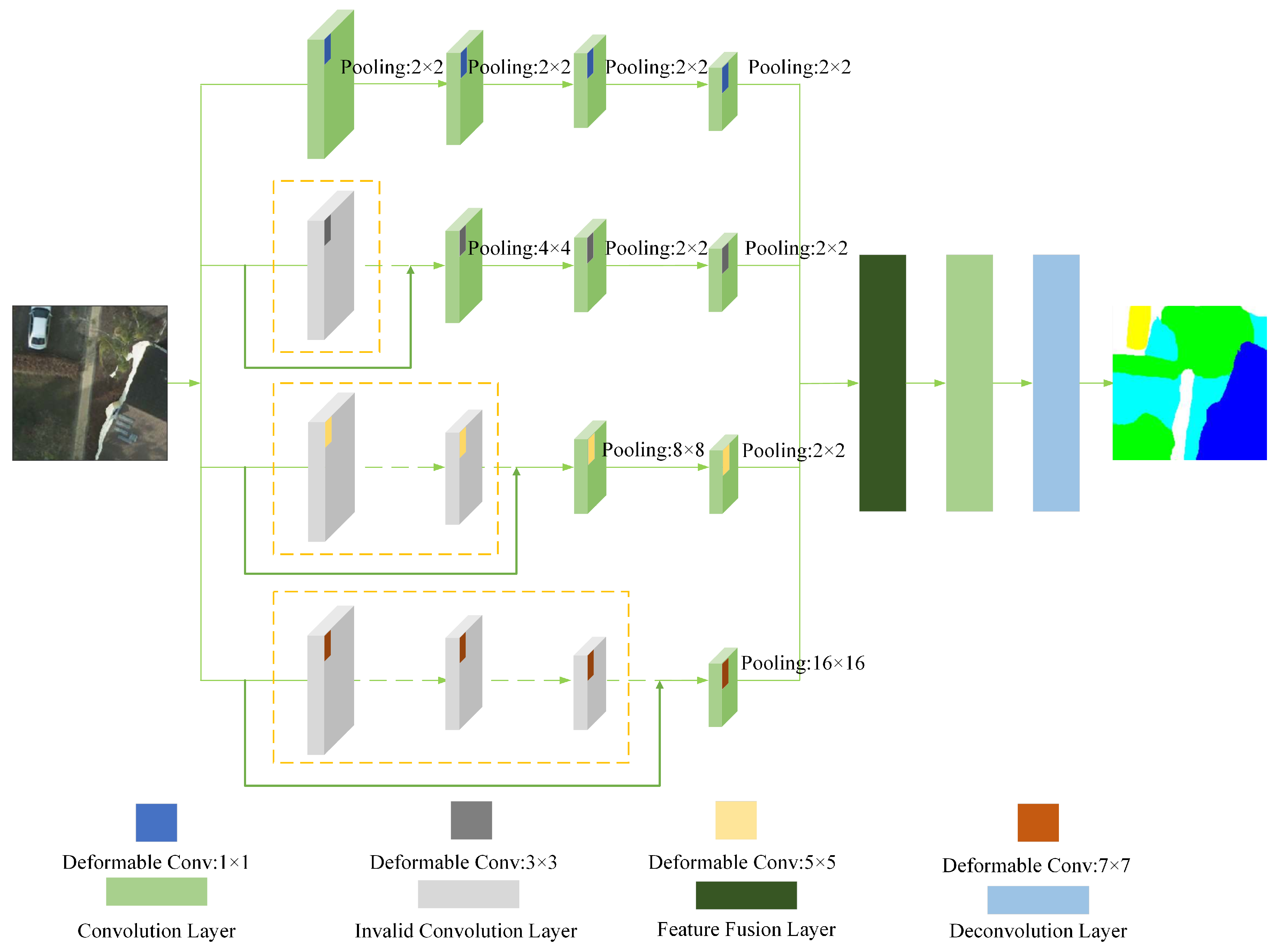
At present, multiscale CNNs can be divided into two types: the multiscale image and the multiscale convolutional kernel. The CNN based on multiscale images feeds images of different resolutions into the neural network with the same size of the convolutional kernel to obtain multiscale features. This method consumes many memory resources due to the need to process multiple images at the same time. The CNN based on the multiscale convolutional kernel feeds the image into several convolutional kernels of different sizes to obtain multiscale features. Due to the introduction of the multiscale convolutional kernels in this structure, the parameter amount of the network is greatly increased, and gradient vanishing is prone to occur during model training. To address the above problems, we proposed a modified multiscale convolutional neural network (mmsCNN) in [45]. In this paper, we combined the previous work and improved it to propose the modified multiscale deformable convolutional neural network (mmsDCNN) model, as shown in Figure 3.
Recently, Reference [49] provided a new perspective: compared with the CNN with a deep large-scale convolutional kernel, the CNN with a shallow large-scale convolutional kernel has a larger receptive field, which is more similar to the human perception mode. In addition, compared with the deep network, the shallow network has fewer parameters, and the problem of gradient disappearance is less likely to occur. Based on this, we integrated the mode of shortcut connections in the residual neural network into the msCNN based on a multiscale convolutional kernel. The proposed model consists of several various deformable convolutional kernel CNNs, i.e., , , , and . Concretely, denotes the CNN with deformable convolutional kernel size = , padding = i, and stride = j. Then, we invalidated the first 1, 2, and 3 layers of , , and , respectively, which are shown in the yellow box in Figure 3. We refer to the network layer in the yellow box as the invalid layer, which is where the shortcut connections are performed. Subsequently, we flexibly set the pooling step size of the network layer after the invalid layer, which ensures that the final output scales of different convolutional networks are consistent. To be specific, we set the pooling layers to , , according to the number of invalid layers, as shown in Figure 3. represents the pooling layers with filtersize = , padding = i, and stride = j.
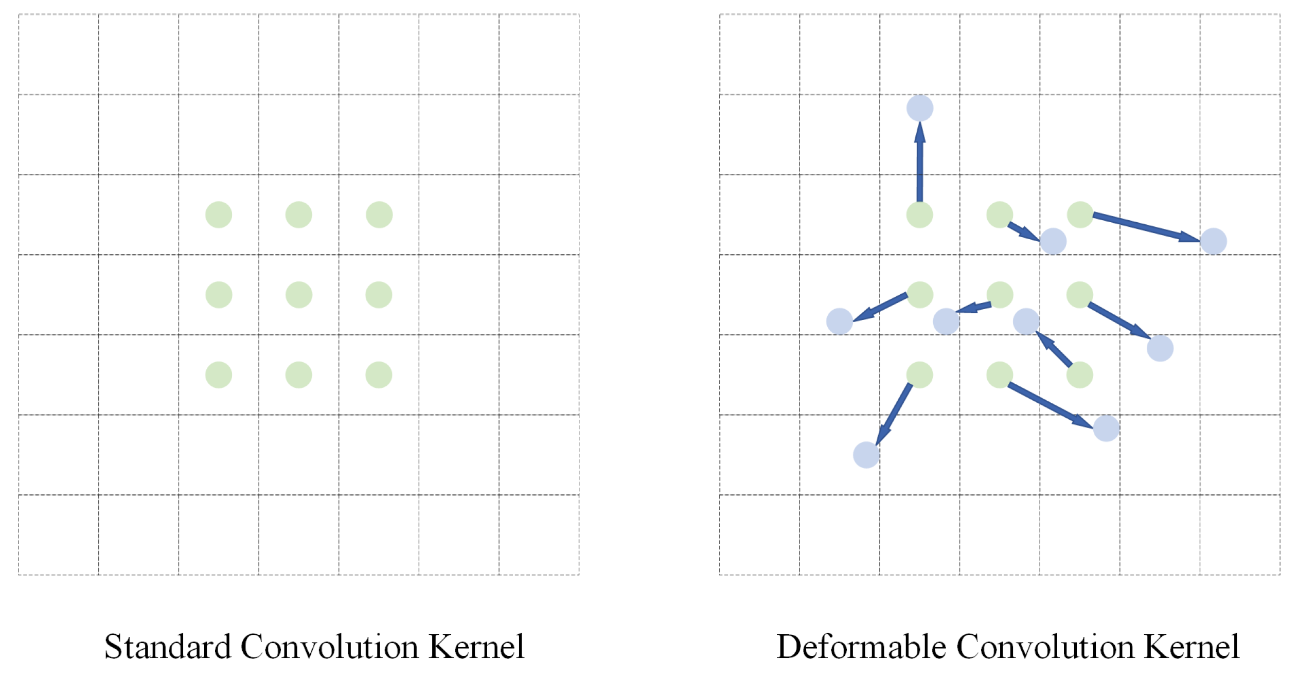
For pixel-level image segmentation tasks, we fused deformable convolution with the mmsCNN model, which can further expand the model’s receptive field. The deformable convolution adds an offset to each convolutional sampling point, which is equivalent to the scalable change in each block of the convolutional kernel, thereby changing the range of the receptive field [50]. Figure 4 compares standard convolutional kernels and deformable convolutional kernels. In the training phase, the convolutional kernel for generating the output features and the convolutional kernel for generating the offsets are learned synchronously. The experiments proved that the mmsDCNN model can consume fewer resources, obtain better experimental results, and effectively avoid gradient disappearance.
Since the feature map gradually becomes smaller during the convolution process, to obtain a feature map with the same size as the original image, we needed to upsample the feature map. An intuitive idea is to perform bilinear interpolation, which is easily implemented with a fixed kernel via deconvolution. Therefore, at the output of the mmsDCNN, we replaced the fully connected network of the mmsCNN model with a deconvolutional network. In addition, before deconvolution, we needed to fuse the multiscale features and then utilize a simple convolution to make the number of channels of the output feature map the same as the predetermined number of categories of the pixels. Notably, the output of the mmsDCNN model is a feature map of the same size as the input image, which will be further processed by DenseCRF to obtain the final prediction map. Table 1 shows the parameter settings of our mmsDCNN model.
2.2. The Multi-Level DenseCRF Model
The conditional random field (CRF) model is a probabilistic undirected graph model, which has recently made great progress in the application of remote sensing image semantic segmentation. In this section, we attempt to utilize DenseCRF to further refine the rough segmentation results output by the mmsDCNN model.
2.2.1. Edge Constraint
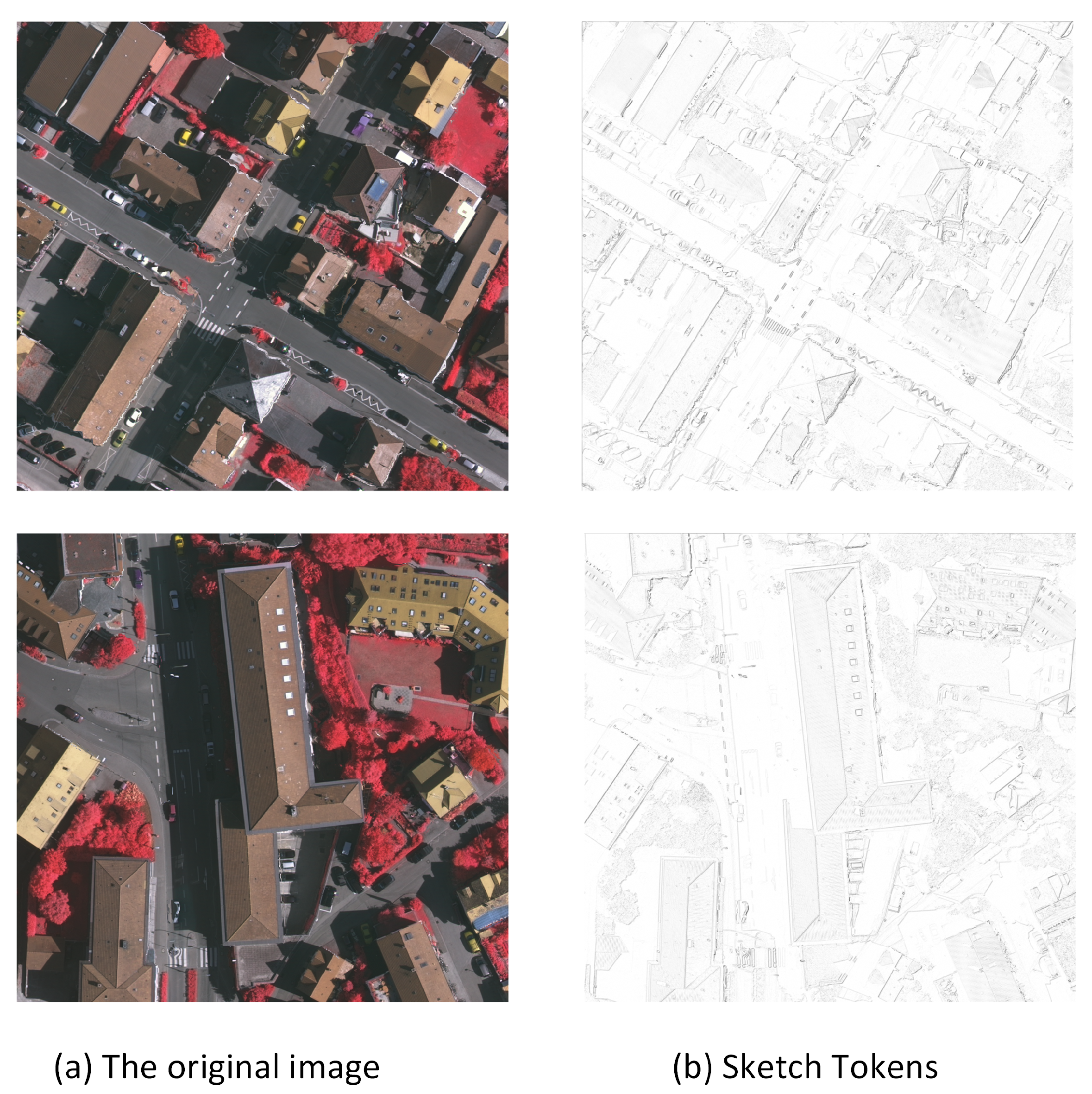
Compared with the pairwise CRF (PCRF) model, which only considers local neighborhood relations, the DenseCRF model is more suitable for image semantic segmentation [46]. It further considers the relationship between each pixel and all other pixels, establishes the dependency on all pixel pairs in the image, and uses the interdependence between pixels to introduce the global information of the image. Although DenseCRF improves the performance of processing image semantic segmentation, it can only determine the region position and approximate shape contour of the object of interest in the image marking results, so there will still be fuzzy edge categories, making it difficult to obtain the real boundary of the segmented region. In order to improve the accuracy of the image segmentation edge, we utilized the Sketch token edge detection algorithm to extract the edge contour features of the image and fused the edge contour features into the potential function of DenseCRF model. The Sketch token edge detection algorithm is a method for learning and detecting image boundary information for mid-level features. It designs Sketch tokens to represent edge structure information in image patches. The input image is first divided into image patches with a size of pixels according to certain rules; then, the Sketch token is used to obtain the channel index features and self-similar features contained in the image patches, and they are finally input into the Structured Random Forest [51] to classify the pixels. Figure 5 shows the edge detection results of some images in the Vaihingen dataset using this algorithm. The Sketch token edge detection algorithm can achieve a similar performance to that of state-of-the-art algorithms, and the global probability of boundary (GPB) [52], sparse code gradients (SCGs) [53], and running speed are greatly improved. For the image to be segmented, let represent the set of image pixels and represent the neighborhood area of the sth pixel. We define the edge energy function as
where is the edge prior parameter, represents the edge constraint item, and and represent the image edge features obtained by the Sketch token edge detection algorithm. For any two pixels, if both are points on the edge or not on the edge, then the penalty of the edge constraint item is 0 to ensure that the segmentation result is not over-segmented or over-smoothed. It is beneficial to maintain the edge constraint of the image; otherwise, we added a marginal penalty to the point. The edge constraint item can increase the constraint on the target segmentation boundary, thereby improving the accuracy of target segmentation.
2.2.2. Combined Multilevel Potential Function
In Section 2.1, we used the mmsDCNN to perform feature extraction on the original image to obtain a preliminary probability map of the same size. In this section, a multi-level DenseCRF based on the superpixel level and pixel level is proposed, which takes the feature map of the mmsDCNN as the input and further utilizes the contextual information of the image at different levels. Notably, the potential energy function of multi-level DenseCRF contains two parts: superpixel-level potential energy function and pixel-level potential energy function.
Firstly, we performed superpixel segmentation on the original image according to the simple linear iterative clustering (SILC) algorithm [54]. In particular, we considered the label of a superpixel to be the category label of most of the pixels in the superpixel. Then, we converted the pixel-level preliminary probability map (feature map) output by the mmsDCNN into a superpixel-level prediction probability map according to the superpixel segmentation map. To be specific, we have
where is the probability distribution of the superpixel, is a superpixel block, is the probability distribution of the nth pixel output by the mmsDCNN model, and N represents the number of most pixels of the same category in a superpixel block. Next, we defined the superpixel-level unary potential function of the DenseCRF model according to the superpixel-level prediction probability map:
Subsequently, we extracted the color feature , spatial feature , and texture feature of the superpixels according to the superpixel segmentation map. The color feature is the average vector of pixels in the CIE-LAB space; the spatial feature is the average vector of the spatial features of all pixels in the superpixel; the texture feature is extracted from the superpixel using the local binary pattern [55]. Then, we defined the superpixel-level binary potential function of the DenseCRF model according to the above superpixel features:
where and are two different superpixel blocks, is the weight parameter on each kernel function, and denotes the superpixel-level feature vectors. The label compatibility function is defined as follows:
To be more exact, the superpixel-level binary potential function of the DenseCRF model can be expanded into
where is the parameter corresponding to the feature.
Superpixel segmentation can not only obtain local feature information, but also better fit the edge contour of the objects. However, the CRF model based on superpixels usually enforces the consistency of the classification labels of all pixels in a superpixel, meaning that the segmentation results are seriously dependent on the quality of the clustering algorithm. To handle this problem, we added the pixel-level potential function constraint term to the superpixel-based Gaussian potential function to obtain a combined Gaussian potential function, which enabled our model to consider features of different granularities and prevent poor superpixel segmentation results from making the output of the model worse.
We defined a pixel-level unary potential function based on the pixel-level probability prediction map that was output by the mmsDCNN model:
where is the probability distribution of pixel . Only the characteristics of a single independent pixel are considered in the unary potential energy term, so the result of image segmentation is often not smooth and contains noise. Therefore, we extracted pixel-level color feature and spatial feature from the original image and then constructed a pixel-level binary potential function. Similarly, the pixel-level binary potential function can be written as
where is the parameter corresponding to the feature and is the edge energy function defined in Equation (1).
To more accurately model the high-dimensional complex features of images, we introduced a high-order potential energy term based on the robust Potts model [56]:
where
is the number of pixels that do not take the main part of the label in subcluster c, indicates the number of pixels in subcluster c, is the number of pixels in subcluster c with class value l:
represents the segmentation quality of subcluster c, is the model parameter, and Q is the truncation parameter.
Finally, we obtained the multi-level DenseCRF based on the superpixel level and pixel level, and its potential function can be expressed as
where V is the set of all superpixels in the image, represents the neighborhood area of the ith pixel, S is the set of all pixels in the image, and C is a set of all subclusters c in the image. The multi-level DenseCRF can consider features of different scales for segmentation, increase the effective constraints on the image target boundary, and improve the accuracy of image segmentation edges. Ultimately, DenseCRF optimizes the rough segmentation result of the mmsDCNN, such as edge thinning and precision machining, to obtain a refined segmentation image.
3. Experiment
To demonstrate the performance of the proposed model, we conducted a series of experiments using the publicly available Potsdam and Vaihingen datasets. In this section, we first provide a brief introduction to the Potsdam and Vaihingen datasets. Next, we describe the experimental parameter settings and evaluation criteria in detail. Finally, we compare the performance with several state-of-the-art models according to the evaluation criteria.
3.1. Datasets
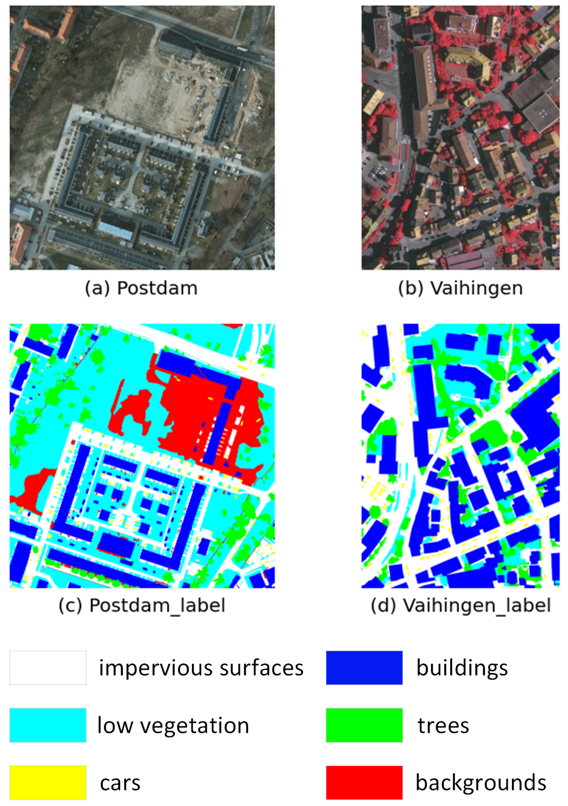
The International Society for Photogrammetry and Remote Sensing (ISPRS) [48] dataset provides two state-of-the-art aerial image datasets for the urban classification and 3D building reconstruction test projects. This dataset employs digital surface models (DSMs) generated from high-resolution orthophotos and corresponding dense image matching techniques. Both datasets cover urban scenes, and each dataset is manually classified into six common land cover classes: impervious surfaces, buildings, low vegetation, trees, cars, and backgrounds. The background class includes water and objects distinct from other defined classes (e.g., containers, tennis courts, swimming pools), which usually belong to uninteresting semantic objects in urban scenes. The Vaihingen dataset contains 33 remote sensing images of different sizes; each image was extracted from a larger, top-level orthophoto image with a spatial resolution of 9 cm. The Potsdam dataset contains 38 image regions of the same size with a spatial resolution of 5 cm. We present several images from the Potsdam and Vaihingen datasets and their corresponding ground truth images in Figure 6, respectively. Due to the memory limitations of the experimental equipment, it was not possible to directly train and infer on the entire image. This paper used the technique in [57] to cut the original data into small pieces before use, keeping the structure of the objects in the images unchanged. We cut the image into a size of with an overlap of 72 and 192 pixels in the training and testing datasets to prevent the loss of information.
3.2. Setting of the Experiments and Evaluation Metrics
For the training and testing setting, 19 images in the Potsdam dataset were selected as the training set, 5 images as the validation set, and 14 images as the testing set. In addition, 13 images were chosen in the Vaihingen dataset as the training set, 3 images as the validation set, and the remaining 17 images as the testing set. We obtained the classification results of 10 groups of parameters on the training set and the validation set and selected the group with the best effect as the final parameters of our model. Table 2 reports the parameters of experimental datasets. The experimental environment is shown in Table 3.
For the parameter settings, the learning rate was initialized to 0.001. The batch size was set to 8. The kernel parameters of multi-level DenseCRF and the weight parameters corresponding to each kernel function were obtained by the grid search method [46].
To more accurately and objectively evaluate the performance of different models, the overall accuracy (OA), precision, recall, F1 [58], and mean intersection over union (mIoU) were selected as our evaluation criteria. The above evaluation parameters can be calculated by the following formulas:
where , , , and are the number of true positives, true negatives, false positives, and false negatives of pixels in the model output image, respectively.
3.3. Experimental Results
3.3.1. Experimental Results on the Potsdam Dataset
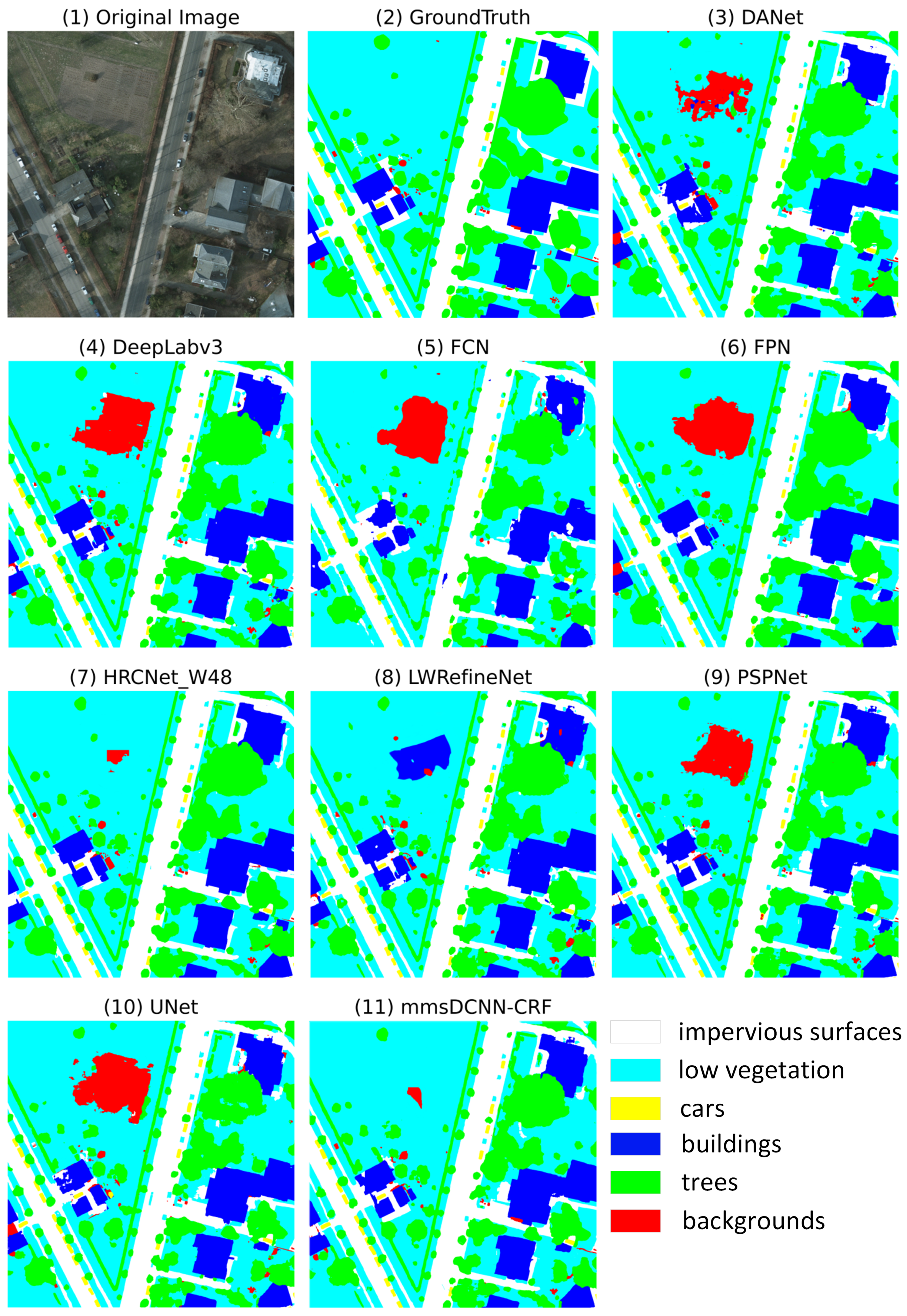
First of all, the experiments were conducted on the Potsdam dataset. The methods FCN [59], PSPNet [40], FPN [60], UNet [39], DeepLabv3 [61], DANet [62], LWRefineNet [63], and HRCNet [18] were chosen for comparison. Table 4 reports their overall accuracies (OA), precision, recall, and F1. In particular, the bold font represents the best indicator.
It is clear from the results our proposed model showed the best performance on the Potsdam dataset. Compared with the HRCNet-W48 model with excellent performance, the model proposed in this paper improved by 0.82% the recall index, 0.75% the precision index, 0.72% the F1 scores, and 0.92% the overall accuracies (OAs). The experimental results verified that the combined model of the multiscale deformable convolution network and multi-level DenseCRF proposed by us can accurately extract low-level details and high-level semantic features from complex remote sensing images and obtain excellent segmentation results.
Table 5 shows the IoU results for each category for all experimental models on the Potsdam dataset. In particular, the bold font represents the best indicator. Based on the HRCNet-W48 model, the mmsDCNN-DenseCRF model proposed in this paper had an IoU that improved by 1.04% for the “Impervious Surfaces” category, for the “Building” category by 0.68%, for the “Low Vegetation” category by 0.85%, for the “Tree” category by 0.59%, and for the “Car”; category by 0.83%. In sum, the mean IoU (mIoU) of our model was 0.8% higher than that of the HRCNet-W48 model, proving the excellent performance of the proposed model.
Figure 7 shows the experimental results of all experimental models in the Potsdam dataset. Compared with the ground truth given in the dataset, the mmsDCNN-DenseCRF model proposed in this paper not only considers the edge information of large objects in the graph, but can also distinguish the details of small objects, which has an indelible relationship with the edge constraint added in the multi-level DenseCRF.
3.3.2. Experimental Results on the Vaihingen Dataset
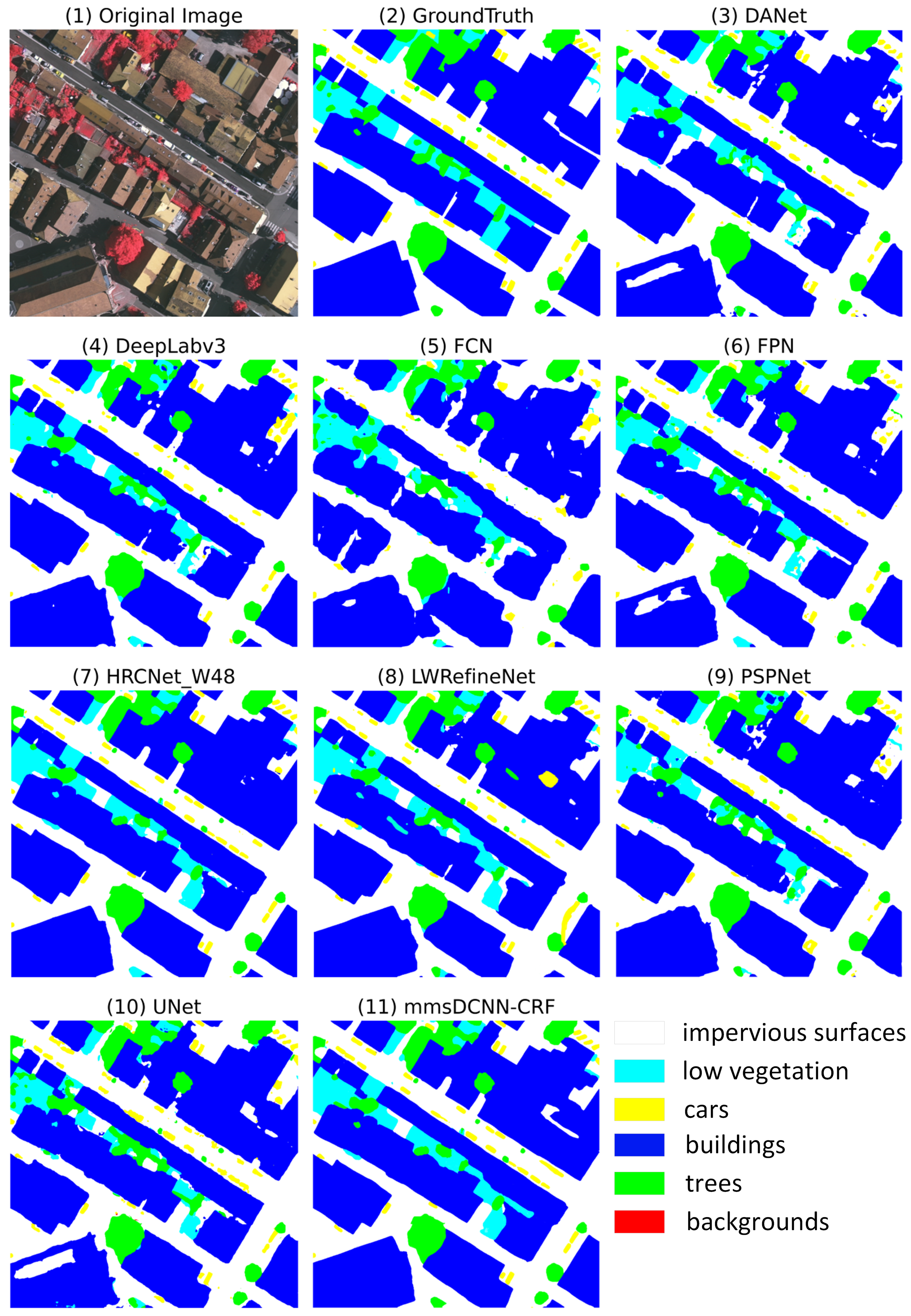
In the second part of the experiment, we replaced the dataset with the Vaihingen dataset in the ISPRS. Analogously, the models FCN [59], PSPNet [40], FPN [60], UNet [39], DeepLabv3 [61], DANet [62], LWRefineNet [63], and HRCNet [18] were selected for comparison. Table 6 summarizes the overall accuracies (OAs), precision, recall, and F1 of those models. In particular, bold font represents the best indicator.
Similarly, the data in the Table 6 make it clear that the model designed in this paper performed best on the Vaihingen dataset. To be specific, compared with the HRCNet-W48 model with a splendid performance, the model proposed in this paper improved by 0.92% the recall index, 1.07% the precision index, 0.85% the F1 scores, and 0.79% the overall accuracies (OAs). The experimental results showed that the multiscale deformable convolutional network model (mmsDCNN) proposed by us can extract rich multiscale features from remote sensing images, and the multi-level DenseCRF further considers the spatial context information of images and, finally, obtained a satisfactory segmentation image.
Table 7 reports the IoU results for each category for all experimental models on the Vaihingen dataset. In particular, the bold font represents the best indicator. Based on the HRCNet-W48 model, the mmsDCNN-DenseCRF model proposed in this paper showed an IoU that improved by 1.07% for the “Impervious Surfaces” category, for the “Building” category by 0.88%, for the “Low Vegetation” category by 0.91%, for the “Tree” category by 0.82%, and for the “Car” category by 0.93%. In summary, the mean IoU (mIoU) of our model was 0.92% higher than that of the HRCNet-W48 model, which fully verified that our model can also perform image segmentation tasks in Vaihingen dataset.
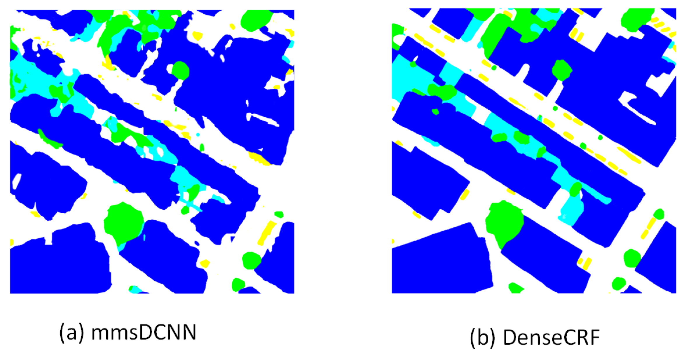
Figure 8 shows the experimental results of all experimental models on the Vaihingen dataset. Compared with all the experimental models, the proposed mmsDCNN-DenseCRF model not only focused on the overall contour of large objects in the image, but can also consider the fine-grained information of small objects, which showed that the mmsDCNN and multi-level DenseCRF can extract multiscale features and grasp the context of the information in the image. In addition, Figure 9 compares the initial segmentation map of the mmsDCNN and the semantic segmentation map of multi-level DenseCRF, which further verified the importance of the multi-level DenseCRF.
3.4. Robustness Verification
To further evaluate the stability of the proposed model, the robustness verification experiment was performed on the Potsdam dataset. According to the method proposed in [35], salt-and-pepper noise and Gaussian noise were randomly added to the testing image, where the salt-and-pepper noise ratio was 0.05 and the mean value and variance of the Gaussian noise were 0 and 0.05. Table 8 reports the experimental results for the damaged Potsdam testing set. According to the experimental results, although the performance of the proposed model declined, it was still acceptable. As a consequence, the robustness of the proposed model was verified by this experiment, and the importance of image denoising algorithm research was also illustrated.
4. Discussion
4.1. Complexity Analysis
In this part, we compared the number of parameters of all models in the experiment. In addition, we used the floating point operations per seconds (FLOPs) to compare the complexity of all experimental models. Table 9 reports the number of parameters and FLOPs of all experimental models on the Potsdam dataset. Particularly, the bold fonts indicate the best indicator.
According to Table 9, although the parameter quantities of the model proposed in this paper were not the lowest, they were superior to most of the models. We had 14.4 M, 2.6 M, and 2 M more parameters than FCN [59], FPN [60], and UNet [39], respectively, but the overall accuracy (OA) of the proposed model was the highest. Additionally, compared with DeepLabv3 [61], LWRefineNet [63], and HRCNet-W48 [18] the parameter quantities of the proposed model were reduced. Compared with PSPNet [40] and DANet [62], the parameter quantities of our model were nearly 17 M less. As shown in Table 9, the FLOPs of the proposed model were superior to most of the experimental methods. In conclusion, the mmsDCNN-DenseCRF can achieve a satisfactory balance between the segmentation performance and the complexity of the model.
4.2. Improvements and Future Work
Considering the problems of deep learning models in the semantic segmentation of remote sensing images, this paper proposed the mmsDCNN-DenseCRF model. The proposed model mainly has the following contributions and improvements. First of all, the modified multiscale deformable convolutional neural network (mmsDCNN) was proposed for multiscale feature extraction. The mmsDCNN model can achieve a balance between strong multiscale feature extraction performance and low computational complexity. Secondly, a multi-level DenseCRF model integrating edge information was designed to complete the optimization task of complex remote sensing image semantic segmentation. Specifically, it can further consider the global context information in the remote sensing image at different granularities, which makes up for the shortcomings of the neural network. Besides, the DenseCRF model incorporating edge information can more accurately restore the outline of objects. The mmsDCNN-DenseCRF model has a clear division of labor and fully considers the main factors that affect the semantic segmentation effect of remote sensing images, such as multiscale feature extraction, spatial context information, and boundary information. Finally, this paper provided a new idea for the semantic segmentation of remote sensing images. Concretely, in the semantic segmentation task of remote sensing images, the learning and reasoning capabilities in the probabilistic graphical model (PGM) can be fully utilized to reduce the burden of deep neural networks and improve the performance of the segmentation model. The numerical experiments on the Potsdam and Vaihingen datasets verified that the segmentation accuracy of the proposed model was about 1% higher than that of the most-advanced model.
In addition to realizing and demonstrating this effect using a specific model, this article hopes to provide a way to solve the problem. In fact, if a feature extractor with better performance appears in the future, the experimental effect may be better, but the idea proposed in this paper is still applicable at that time. Therefore, our next step is to improve and integrate the feature extraction model with a stronger multiscale feature extraction capability and less computational complexity with the semantic segmentation model used in this paper, such as the new modified YOLOv3 model with four scale detection layers [38], which shows an excellent multiscale feature extraction performance. Furthermore, in future experiments, we will further extend the model experiments to explore multi-spectral remote sensing data.
5. Conclusions
Considering the main factors affecting the semantic segmentation of remote sensing images and the problems of deep learning models in the semantic segmentation of remote sensing images, this paper proposed the mmsDCNN-DenseCRF model. First of all, a lightweight multiscale deformable convolution network (mmsDCNN) was designed to generate a preliminary prediction probability map. The mmsDCNN model was improved on the basis of the CNN and can achieve a balance between strong multiscale feature extraction capabilities and less computational complexity. Then, a multi-level DenseCRF based on the superpixel level and pixel level was proposed as an optimization module, which can make full use of the image context information at different granularities in the decoding process to obtain more precise semantic segmentation results. In addition, to better recover the contour of the object, the Sketch token edge detection algorithm was utilized to extract the edge contour features of the image, and the edge contour features were fused into the Gaussian edge potential function of the DenseCRF model. In sum, the mmsDCNN-DenseCRF model comprehensively considers several main factors that affect the semantic segmentation effect of remote sensing images, including multiscale feature extraction, spatial context information, and boundary information. In particular, the proposed model can strike a balance between satisfactory segmentation performance and low complexity. Finally, the numerical experiments on the Potsdam and Vaihingen datasets verified that the proposed model is superior to the most-advanced model.
Author Contributions
Methodology, X.C.; formal analysis, X.C.; investigation, X.C.; writing—original draft preparation, X.C.; writing—review and editing, X.C. and H.L.; visualization, X.C. and H.L.; supervision, H.L.; project administration, H.L. All authors have read and agreed to the published version of the manuscript.
Funding
This research received no external funding.
Data Availability Statement
Datasets relevant to our paper are available online.
Conflicts of Interest
The authors declare no conflict of interest.
References
- Csurka, G.; Perronnin, F. An efficient approach to semantic segmentation. Int. J. Comput. Vis. 2011, 95, 198–212. [Google Scholar] [CrossRef]
- Zhu, X.X.; Tuia, D.; Mou, L.; Xia, G.S.; Zhang, L.; Xu, F.; Fraundorfer, F. Deep learning in remote sensing: A comprehensive review and list of resources. IEEE Geosci. Remote Sens. Mag. 2017, 5, 8–36. [Google Scholar] [CrossRef] [Green Version]
- Li, Y.; Tao, C.; Tan, Y.; Shang, K.; Tian, J. Unsupervised multilayer feature learning for satellite image scene classification. IEEE Geosci. Remote Sens. Lett. 2016, 13, 157–161. [Google Scholar] [CrossRef]
- Li, Y.; Ma, J.; Zhang, Y. Image retrieval from remote sensing big data: A survey. Inf. Fusion 2021, 67, 94–115. [Google Scholar] [CrossRef]
- Zhang, L.; Zhang, L.; Du, B. Deep learning for remote sensing data: A technical tutorial on the state of the art. IEEE Geosci. Remote Sens. Mag. 2016, 4, 22–40. [Google Scholar] [CrossRef]
- Ma, L.; Liu, Y.; Zhang, X.; Ye, Y.; Yin, G.; Johnson, B.A. Deep learning in remote sensing applications: A meta-analysis and review. Isprs J. Photogramm. Remote Sens. 2019, 152, 166–177. [Google Scholar] [CrossRef]
- Li, Y.; Chen, W.; Zhang, Y.; Tao, C.; Xiao, R.; Tan, Y. Accurate cloud detection in high-resolution remote sensing imagery by weakly supervised deep learning. Remote Sens. Environ. 2020, 250, 112045. [Google Scholar] [CrossRef]
- Li, Y.; Zhang, Y.; Huang, X.; Yuille, A.L. Deep networks under scene-level supervision for multi-class geospatial object detection from remote sensing images. Isprs J. Photogramm. Remote Sens. 2018, 146, 182–196. [Google Scholar] [CrossRef]
- Gu, W.; Bai, S.; Kong, L. A review on 2D instance segmentation based on deep neural networks. Image Vis. Comput. 2022, 120, 104401. [Google Scholar] [CrossRef]
- Elharrouss, O.; Al-Maadeed, S.; Subramanian, N.; Ottakath, N.; Almaadeed, N.; Himeur, Y. Panoptic segmentation: A review. arXiv 2021, arXiv:2111.10250. [Google Scholar]
- Hafiz, A.M.; Bhat, G.M. A survey on instance segmentation: State of the art. Int. J. Multimed. Inf. Retr. 2020, 9, 171–189. [Google Scholar] [CrossRef]
- Bolya, D.; Zhou, C.; Xiao, F.; Lee, Y.J. Yolact: Real-time instance segmentation. In Proceedings of the IEEE/CVF International Conference on Computer Vision, Seoul, Republic of Korea, 27 October–2 November 2019; pp. 9157–9166. [Google Scholar]
- Tian, Z.; Shen, C.; Chen, H. Conditional convolutions for instance segmentation. In Proceedings of the Computer Vision–ECCV 2020: 16th European Conference, Glasgow, UK, 23–28 August 2020; Proceedings, Part I 16. Springer: Berlin, Germany, 2020; pp. 282–298. [Google Scholar]
- Kirillov, A.; He, K.; Girshick, R.; Rother, C.; Dollár, P. Panoptic segmentation. In Proceedings of the IEEE/CVF Conference on Computer Vision and Pattern Recognition, Long Beach, CA, USA, 15–20 June 2019; pp. 9404–9413. [Google Scholar]
- Li, X.; Chen, D. A survey on deep learning-based panoptic segmentation. Digit. Signal Process. 2022, 120, 103283. [Google Scholar] [CrossRef]
- Li, Y.; Chen, X.; Zhu, Z.; Xie, L.; Huang, G.; Du, D.; Wang, X. Attention-guided unified network for panoptic segmentation. In Proceedings of the IEEE/CVF Conference on Computer Vision and Pattern Recognition, Long Beach, CA, USA, 15–20 June 2019; pp. 7026–7035. [Google Scholar]
- Tasar, O.; Tarabalka, Y.; Alliez, P. Incremental learning for semantic segmentation of large-scale remote sensing data. IEEE J. Sel. Top. Appl. Earth Obs. Remote Sens. 2019, 12, 3524–3537. [Google Scholar] [CrossRef] [Green Version]
- Xu, Z.; Zhang, W.; Zhang, T.; Li, J. HRCNet: High-resolution context extraction network for semantic segmentation of remote sensing images. Remote Sens. 2020, 13, 71. [Google Scholar] [CrossRef]
- Rublee, E.; Rabaud, V.; Konolige, K.; Bradski, G. ORB: An efficient alternative to SIFT or SURF. In Proceedings of the 2011 International Conference on Computer Vision, Barcelona, Spain, 6–13 November 2011; IEEE: New York, NY, USA, 2011; pp. 2564–2571. [Google Scholar]
- Pietikäinen, M. Local binary patterns. Scholarpedia 2010, 5, 9775. [Google Scholar] [CrossRef]
- Bay, H.; Ess, A.; Tuytelaars, T.; Van Gool, L. Speeded-up robust features (SURF). Comput. Vis. Image Underst. 2008, 110, 346–359. [Google Scholar] [CrossRef]
- Noble, W.S. What is a support vector machine? Nat. Biotechnol. 2006, 24, 1565–1567. [Google Scholar] [CrossRef]
- Kleinbaum, D.G.; Dietz, K.; Gail, M.; Klein, M.; Klein, M. Logistic Regression; Springer: Berlin, Germany, 2002. [Google Scholar]
- Han, K.; Guo, J.; Zhang, C.; Zhu, M. Attribute-aware attention model for fine-grained representation learning. In Proceedings of the 26th ACM International Conference on Multimedia, Seoul, Republic of Korea, 22–26 October 2018; pp. 2040–2048. [Google Scholar]
- Hinton, G.E.; Salakhutdinov, R.R. Reducing the dimensionality of data with neural networks. Science 2006, 313, 504–507. [Google Scholar] [CrossRef] [Green Version]
- Li, S.; Song, W.; Fang, L.; Chen, Y.; Ghamisi, P.; Benediktsson, J.A. Deep learning for hyperspectral image classification: An overview. IEEE Trans. Geosci. Remote Sens. 2019, 57, 6690–6709. [Google Scholar] [CrossRef] [Green Version]
- Affonso, C.; Rossi, A.L.D.; Vieira, F.H.A.; de Leon Ferreira, A.C.P. Deep learning for biological image classification. Expert Syst. Appl. 2017, 85, 114–122. [Google Scholar] [CrossRef] [Green Version]
- Oprea, S.; Martinez-Gonzalez, P.; Garcia-Garcia, A.; Castro-Vargas, J.A.; Orts-Escolano, S.; Garcia-Rodriguez, J.; Argyros, A. A review on deep learning techniques for video prediction. IEEE Trans. Pattern Anal. Mach. Intell. 2022, 44, 2806–2826. [Google Scholar] [CrossRef] [PubMed]
- Oh, J.; Guo, X.; Lee, H.; Lewis, R.L.; Singh, S. Action-conditional video prediction using deep networks in atari games. Adv. Neural Inf. Process. Syst. 2015, 28. [Google Scholar] [CrossRef]
- Khan, S.; Rahmani, H.; Shah, S.A.A.; Bennamoun, M. A guide to convolutional neural networks for computer vision. Synth. Lect. Comput. Vis. 2018, 8, 1–207. [Google Scholar]
- Liu, Z.; Yeoh, J.K.; Gu, X.; Dong, Q.; Chen, Y.; Wu, W.; Wang, L.; Wang, D. Automatic pixel-level detection of vertical cracks in asphalt pavement based on GPR investigation and improved mask R-CNN. Autom. Constr. 2023, 146, 104689. [Google Scholar] [CrossRef]
- Wang, P.; Zhao, H.; Yang, Z.; Jin, Q.; Wu, Y.; Xia, P.; Meng, L. Fast Tailings Pond Mapping Exploiting Large Scene Remote Sensing Images by Coupling Scene Classification and Sematic Segmentation Models. Remote Sens. 2023, 15, 327. [Google Scholar] [CrossRef]
- Wang, X.; Cheng, W.; Feng, Y.; Song, R. TSCNet: Topological Structure Coupling Network for Change Detection of Heterogeneous Remote Sensing Images. Remote Sens. 2023, 15, 621. [Google Scholar] [CrossRef]
- Zhang, X.; Zhou, Y.; Qiao, P.; Lv, X.; Li, J.; Du, T.; Cai, Y. Image Registration Algorithm for Remote Sensing Images Based on Pixel Location Information. Remote Sens. 2023, 15, 436. [Google Scholar] [CrossRef]
- Wang, D.; Liu, Z.; Gu, X.; Wu, W.; Chen, Y.; Wang, L. Automatic detection of pothole distress in asphalt pavement using improved convolutional neural networks. Remote Sens. 2022, 14, 3892. [Google Scholar] [CrossRef]
- Ding, L.; Zhang, J.; Bruzzone, L. Semantic segmentation of large-size VHR remote sensing images using a two-stage multiscale training architecture. IEEE Trans. Geosci. Remote Sens. 2020, 58, 5367–5376. [Google Scholar] [CrossRef]
- Diakogiannis, F.I.; Waldner, F.; Caccetta, P.; Wu, C. ResUNet-a: A deep learning framework for semantic segmentation of remotely sensed data. Isprs J. Photogramm. Remote Sens. 2020, 162, 94–114. [Google Scholar] [CrossRef] [Green Version]
- Liu, Z.; Gu, X.; Chen, J.; Wang, D.; Chen, Y.; Wang, L. Automatic recognition of pavement cracks from combined GPR B-scan and C-scan images using multiscale feature fusion deep neural networks. Autom. Constr. 2023, 146, 104698. [Google Scholar] [CrossRef]
- Ronneberger, O.; Fischer, P.; Brox, T. U-net: Convolutional networks for biomedical image segmentation. In Proceedings of the International Conference on Medical Image Computing and Computer-Assisted Intervention, Munich, Germany, 5–9 October 2015; Springer: Berlin, Germany, 2015; pp. 234–241. [Google Scholar]
- Zhao, H.; Shi, J.; Qi, X.; Wang, X.; Jia, J. Pyramid scene parsing network. In Proceedings of the IEEE Conference on Computer Vision and Pattern Recognition, Honolulu, HI, USA, 21–26 July 2017; pp. 2881–2890. [Google Scholar]
- Sun, K.; Xiao, B.; Liu, D.; Wang, J. Deep high-resolution representation learning for human pose estimation. In Proceedings of the IEEE/CVF Conference on Computer Vision and Pattern Recognition, Long Beach, CA, USA, 15–20 June 2019; pp. 5693–5703. [Google Scholar]
- Takikawa, T.; Acuna, D.; Jampani, V.; Fidler, S. Gated-scnn: Gated shape cnns for semantic segmentation. In Proceedings of the IEEE/CVF International Conference on Computer Vision, Seoul, Republic of Korea, 27 October–2 November 2019; IEEE: New York, NY, USA; pp. 5229–5238. [Google Scholar]
- Li, R.; Zheng, S.; Zhang, C.; Duan, C.; Su, J.; Wang, L.; Atkinson, P.M. Multiattention network for semantic segmentation of fine-resolution remote sensing images. IEEE Trans. Geosci. Remote Sens. 2021, 60, 1–13. [Google Scholar] [CrossRef]
- Hamida, A.B.; Benoit, A.; Lambert, P.; Klein, L.; Amar, C.B.; Audebert, N.; Lefèvre, S. Deep learning for semantic segmentation of remote sensing images with rich spectral content. In Proceedings of the 2017 IEEE International Geoscience and Remote Sensing Symposium (IGARSS), Fort Worth, TX, USA, 23–28 July 2017; IEEE: New York, NY, USA, 2017; pp. 2569–2572. [Google Scholar]
- Cheng, X.; Lei, H. Remote sensing scene image classification based on mmsCNN–HMM with stacking ensemble model. Remote Sens. 2022, 14, 4423. [Google Scholar] [CrossRef]
- Krähenbühl, P.; Koltun, V. Efficient Inference in Fully Connected CRFs with Gaussian Edge Potentials. In Proceedings of the Neural Information Processing Systems, Granada, Spain, 12–15 December 2011. [Google Scholar]
- Lim, J.J.; Zitnick, C.L.; Dollár, P. Sketch tokens: A learned mid-level representation for contour and object detection. In Proceedings of the IEEE Conference on Computer Vision and Pattern Recognition, Portland, OR, USA, 23–28 June 2013; pp. 3158–3165. [Google Scholar]
- Konecny, G. The International Society for Photogrammetry and Remote Sensing (ISPRS) study on the status of mapping in the world. In Proceedings of the International Workshop on “Global Geospatial Information”, Novosibirsk, Russia, 25 April 2013; Citeseer: Novosibirsk, Russian, 2013; pp. 4–24. [Google Scholar]
- Ding, X.; Zhang, X.; Han, J.; Ding, G. Scaling up your kernels to 31x31: Revisiting large kernel design in cnns. In Proceedings of the IEEE/CVF Conference on Computer Vision and Pattern Recognition, New Orleans, LA, USA, 18–24 June 2022; pp. 11963–11975. [Google Scholar]
- Dai, J.; Qi, H.; Xiong, Y.; Li, Y.; Zhang, G.; Hu, H.; Wei, Y. Deformable convolutional networks. In Proceedings of the IEEE International Conference on Computer Vision, Venice, Italy, 22–29 October 2017; pp. 764–773. [Google Scholar]
- Dollár, P.; Zitnick, L.C. Structured Forests for Fast Edge Detection. In Proceedings of the IEEE International Conference on Computer Vision, Sydney, Australia, 1–8 December 2013. [Google Scholar]
- Arbelaez, P.; Maire, M.; Fowlkes, C.; Malik, J. Contour detection and hierarchical image segmentation. IEEE Trans. Pattern Anal. Mach. Intell. 2010, 33, 898–916. [Google Scholar] [CrossRef] [PubMed] [Green Version]
- Xiaofeng, R.; Bo, L. Discriminatively trained sparse code gradients for contour detection. Adv. Neural Inf. Process. Syst. 2012, 25, 584–592. [Google Scholar]
- Achanta, R.; Shaji, A.; Smith, K.; Lucchi, A.; Fua, P.; Süsstrunk, S. SLIC superpixels compared to state-of-the-art superpixel methods. IEEE Trans. Pattern Anal. Mach. Intell. 2012, 34, 2274–2282. [Google Scholar] [CrossRef] [PubMed] [Green Version]
- Ojala, T.; Pietikainen, M.; Maenpaa, T. Multiresolution gray-scale and rotation invariant texture classification with local binary patterns. IEEE Trans. Pattern Anal. Mach. Intell. 2002, 24, 971–987. [Google Scholar] [CrossRef]
- Kohli, P.; Ladický, L.U.; Torr, P.H. Robust higher order potentials for enforcing label consistency. Int. J. Comput. Vis. 2009, 82, 302–324. [Google Scholar] [CrossRef] [Green Version]
- Zhang, J.; Lin, S.; Ding, L.; Bruzzone, L. Multi-scale context aggregation for semantic segmentation of remote sensing images. Remote Sens. 2020, 12, 701. [Google Scholar] [CrossRef] [Green Version]
- Mousavi Kahaki, S.M.; Nordin, M.J.; Ashtari, A.H.; Zahra, S.J. Invariant feature matching for image registration application based on new dissimilarity of spatial features. PLoS ONE 2016, 11, e0149710. [Google Scholar] [CrossRef] [PubMed]
- Long, J.; Shelhamer, E.; Darrell, T. Fully convolutional networks for semantic segmentation. In Proceedings of the IEEE Conference on Computer Vision and Pattern Recognition, Boston, MA, USA, 7–12 June 2015; pp. 3431–3440. [Google Scholar]
- Lin, T.Y.; Dollár, P.; Girshick, R.; He, K.; Hariharan, B.; Belongie, S. Feature pyramid networks for object detection. In Proceedings of the IEEE Conference on Computer Vision and Pattern Recognition, Honolulu, HI, USA, 21–26 July 2017; pp. 2117–2125. [Google Scholar]
- Chen, L.C.; Papandreou, G.; Schroff, F.; Adam, H. Rethinking atrous convolution for semantic image segmentation. arXiv 2017, arXiv:1706.05587. [Google Scholar]
- Fu, J.; Liu, J.; Tian, H.; Li, Y.; Bao, Y.; Fang, Z.; Lu, H. Dual attention network for scene segmentation. In Proceedings of the IEEE/CVF Conference on Computer Vision and Pattern Recognition, Long Beach, CA, USA, 15–20 June 2019; pp. 3146–3154. [Google Scholar]
- Nekrasov, V.; Dharmasiri, T.; Spek, A.; Drummond, T.; Shen, C.; Reid, I. Real-time joint semantic segmentation and depth estimation using asymmetric annotations. In Proceedings of the 2019 International Conference on Robotics and Automation (ICRA), Montreal, QC, Canada, 20–24 May 2019; IEEE: New York, NY, USA, 2019; p. 7101. [Google Scholar]
Figure 1.
The figure shows the inter-class similarity and intra-class variability of remote sensing images.
Figure 1.
The figure shows the inter-class similarity and intra-class variability of remote sensing images.

Figure 2.
The figure shows the basic framework of the proposed model.

Figure 3.
The framework of the modified multiscale deformable convolutional neural network (mmsDCNN).
Figure 3.
The framework of the modified multiscale deformable convolutional neural network (mmsDCNN).

Figure 4.
The figure compares standard convolutional kernels and deformable convolutional kernels.

Figure 5.
The figure shows the edge detection results of some images in the Vaihingen dataset using Sketch token edge detection algorithm.
Figure 5.
The figure shows the edge detection results of some images in the Vaihingen dataset using Sketch token edge detection algorithm.

Figure 6.
(a) Sample image of Potsdam dataset. (b) Sample image of Vaihingen dataset. (c) Ground truth of sample image of Potsdam dataset. (d) Ground truth of sample image of Vaihingen dataset.
Figure 6.
(a) Sample image of Potsdam dataset. (b) Sample image of Vaihingen dataset. (c) Ground truth of sample image of Potsdam dataset. (d) Ground truth of sample image of Vaihingen dataset.

Figure 7.
The figure shows the experimental results of all experimental models and the ground truth on the Potsdam dataset.
Figure 7.
The figure shows the experimental results of all experimental models and the ground truth on the Potsdam dataset.

Figure 8.
The figure shows the initial segmentation of the mmsDCNN and the segmentation map as estimated from DenseCRF.
Figure 8.
The figure shows the initial segmentation of the mmsDCNN and the segmentation map as estimated from DenseCRF.

Figure 9.
The initial segmentation of the mmsDCNN and the segmentation map as estimated from the DenseCRF.
Figure 9.
The initial segmentation of the mmsDCNN and the segmentation map as estimated from the DenseCRF.


Table 1.
Structure parameters of our mmsDCNN model.
| Type | Number | Filter Size | Pad | Stride |
|---|---|---|---|---|
| Conv1 + ReLU | 32 | 0 | 1 | |
| Max Pooling | − | 0 | 2 | |
| Conv2 + ReLU | 64 | 1 | ||
| Max Pooling | − | 0 | ||
| Conv3 + ReLU | 128 | 1 | ||
| Max Pooling | − | 0 | ||
| Conv4 + ReLU | 256 | 1 | ||
| Max Pooling | − | 0 | ||
| Conv5 + ReLU | 6 | 0 | 1 | |
| Deconv Layer | 6 | 8 | 16 |
Table 2.
Parameters of the experimental dataset.
| Item | Potsdam Training | Potsdam Testing | Vaihingen Training | Vaihingen Testing |
|---|---|---|---|---|
| size (pixel) | ||||
| number | 6931 | 13454 | 654 | 2219 |
| overlap pixels | 72 | 192 | 72 | 192 |
| p pixels | 72 | 192 | 72 | 192 |
Table 3.
The experimental environment.
| The Experimental Environment | Experimental Configuration |
|---|---|
| Processor | |
| GPU | |
| Memory | |
| Operating system | |
| Compiler |
Table 4.
Results for the Potsdam dataset using the above models.
| Model | Recall (%) | Precision (%) | F1 Score (%) | OA (%) |
|---|---|---|---|---|
| FCN [59] | ||||
| PSPNet [40] | ||||
| FPN [60] | ||||
| UNet [39] | ||||
| DeepLabv3 [61] | ||||
| DANet [62] | ||||
| LWRefineNet [63] | ||||
| HRCNet-W48 [18] | ||||
| The proposed model |
Table 5.
The mean intersection over union (%) on the Potsdam dataset with the above models.
| Model | ImSurface | Building | Low Vegetation | Tree | Car | mIoU (%) |
|---|---|---|---|---|---|---|
| FCN [59] | ||||||
| PSPNet [40] | ||||||
| FPN [60] | ||||||
| UNet [39] | ||||||
| DeepLabv3 [61] | ||||||
| DANet [62] | ||||||
| LWRefineNet [63] | ||||||
| HRCNet-W48 [18] | ||||||
| The proposed model |
Table 6.
Results for the Vaihingen dataset with the above models.
| Model | Recall (%) | Precision (%) | F1 Score (%) | OA (%) |
|---|---|---|---|---|
| FCN [59] | ||||
| PSPNet [40] | ||||
| FPN [60] | ||||
| UNet [39] | ||||
| DeepLabv3 [61] | ||||
| DANet [62] | ||||
| LWRefineNet [63] | ||||
| HRCNet-W48 [18] | ||||
| The proposed model |
Table 7.
The mean intersection over union (%) on the Vaihingen dataset with the above models.
| Model | ImSurface | Building | Low Vegetation | Tree | Car | mIoU (%) |
|---|---|---|---|---|---|---|
| FCN [59] | ||||||
| PSPNet [40] | ||||||
| FPN [60] | ||||||
| UNet [39] | ||||||
| DeepLabv3 [61] | ||||||
| DANet [62] | ||||||
| LWRefineNet [63] | ||||||
| HRCNet-W48 [18] | ||||||
| The proposed model |
Table 8.
Results on the damaged Potsdam testing set.
| Model | mIoU (%) | Precision (%) | F1 Score (%) | OA (%) |
|---|---|---|---|---|
| Proposed model | ||||
| Proposed model (salt-and-pepper noise) | ||||
| Proposed model (Gaussian noise) |
Disclaimer/Publisher’s Note: The statements, opinions and data contained in all publications are solely those of the individual author(s) and contributor(s) and not of MDPI and/or the editor(s). MDPI and/or the editor(s) disclaim responsibility for any injury to people or property resulting from any ideas, methods, instructions or products referred to in the content. |
© 2023 by the authors. Licensee MDPI, Basel, Switzerland. This article is an open access article distributed under the terms and conditions of the Creative Commons Attribution (CC BY) license (https://creativecommons.org/licenses/by/4.0/).
Share and Cite
MDPI and ACS Style
Cheng, X.; Lei, H. Semantic Segmentation of Remote Sensing Imagery Based on Multiscale Deformable CNN and DenseCRF. Remote Sens. 2023, 15, 1229. https://doi.org/10.3390/rs15051229
AMA Style
Cheng X, Lei H. Semantic Segmentation of Remote Sensing Imagery Based on Multiscale Deformable CNN and DenseCRF. Remote Sensing. 2023; 15(5):1229. https://doi.org/10.3390/rs15051229
Chicago/Turabian StyleCheng, Xiang, and Hong Lei. 2023. "Semantic Segmentation of Remote Sensing Imagery Based on Multiscale Deformable CNN and DenseCRF" Remote Sensing 15, no. 5: 1229. https://doi.org/10.3390/rs15051229
Note that from the first issue of 2016, this journal uses article numbers instead of page numbers. See further details here.