
SAR and Optical Data Applied to Early-Season Mapping of Integrated Crop–Livestock Systems Using Deep and Machine Learning Algorithms
 , ,
, ,  , , , , and
Abstract
:
1. Introduction
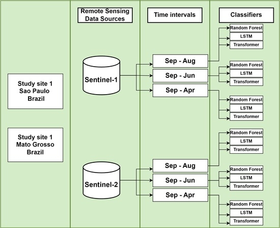
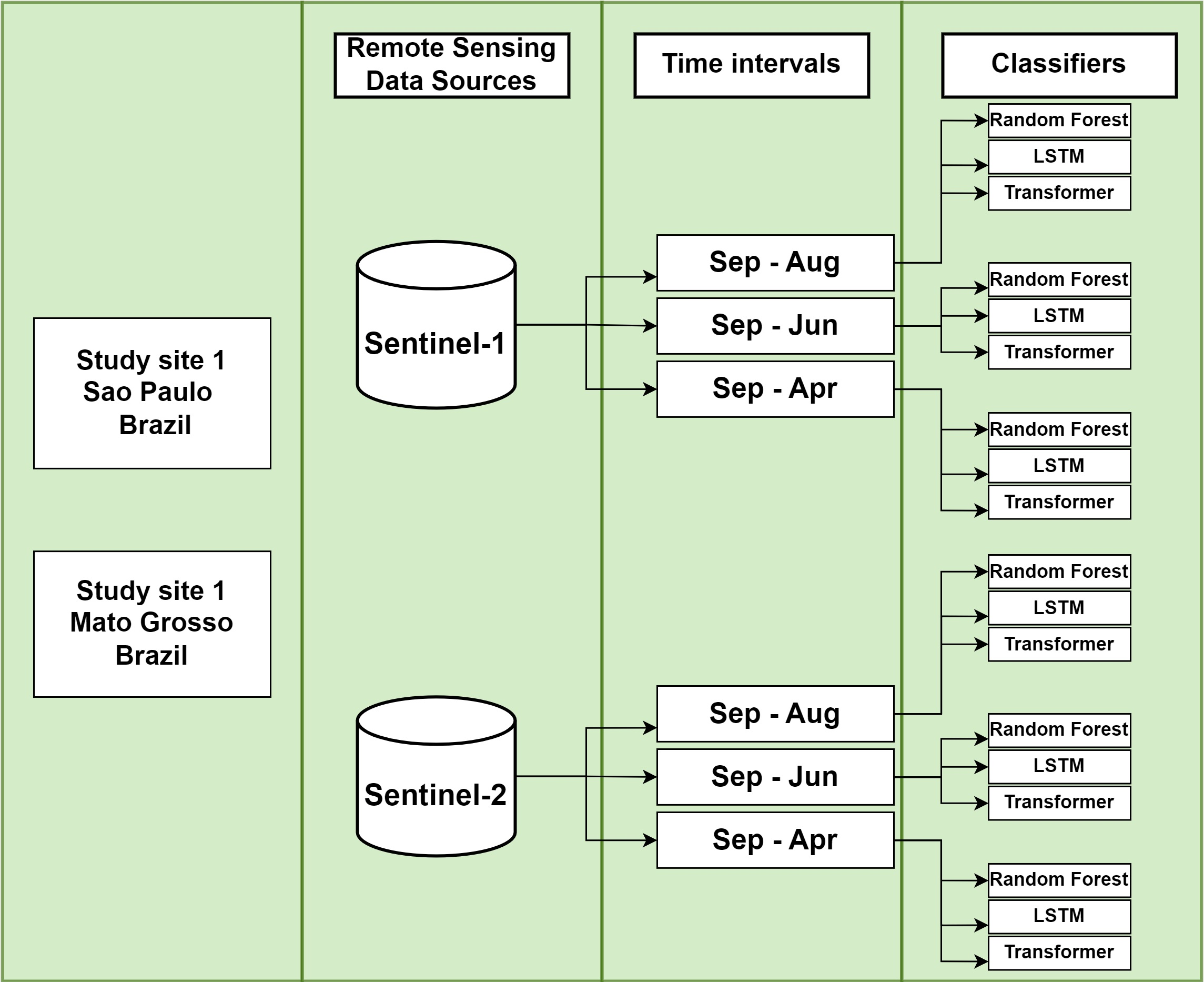
2. Materials and Methods
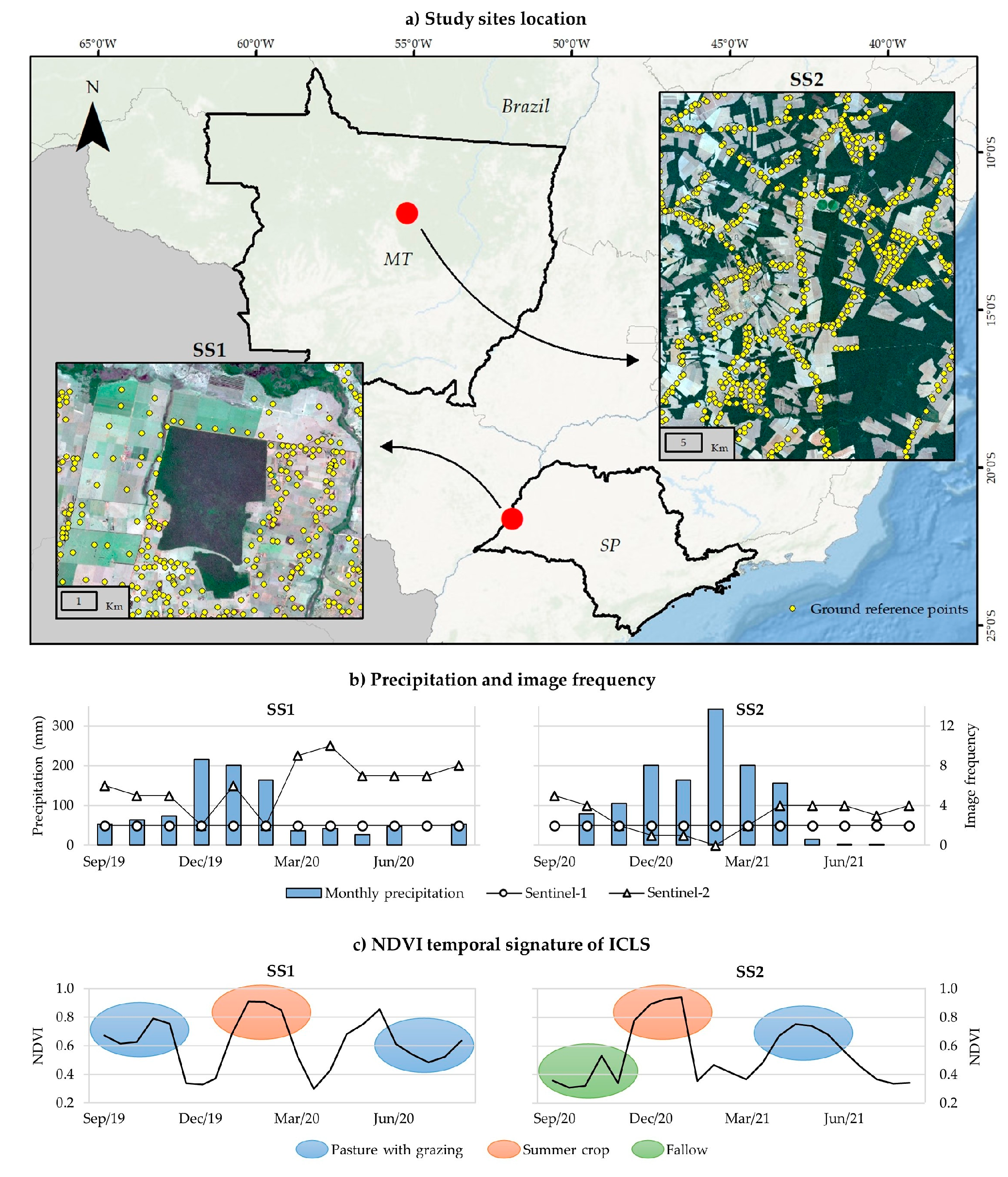
2.1. Study Sites
2.2. Field Data Collection
2.3. Remote Sensing Data Collection and Preprocessing
2.4. Multitemporal Segmentation
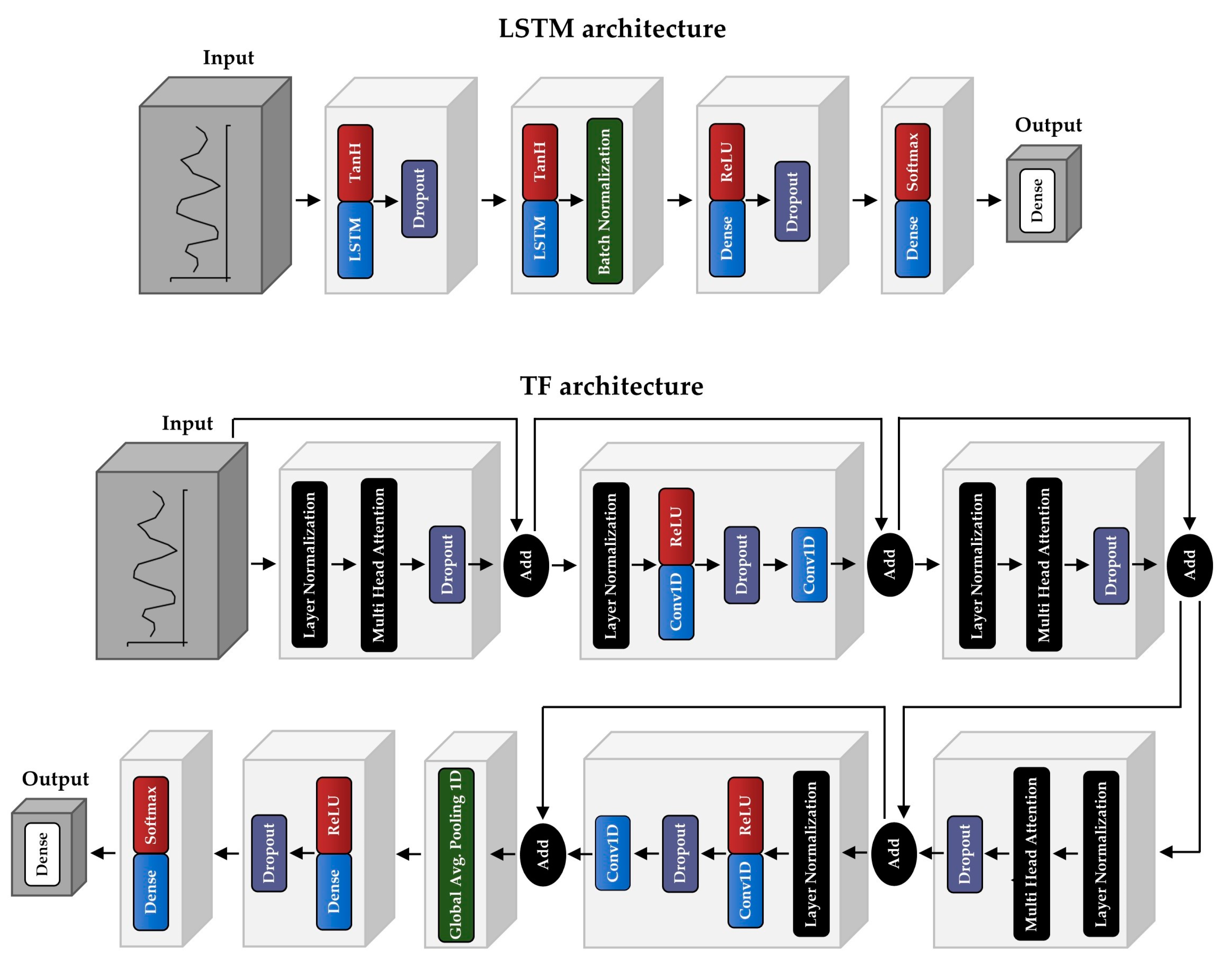
2.5. Machine and Deep Learning Algorithms
2.6. Results Evaluation
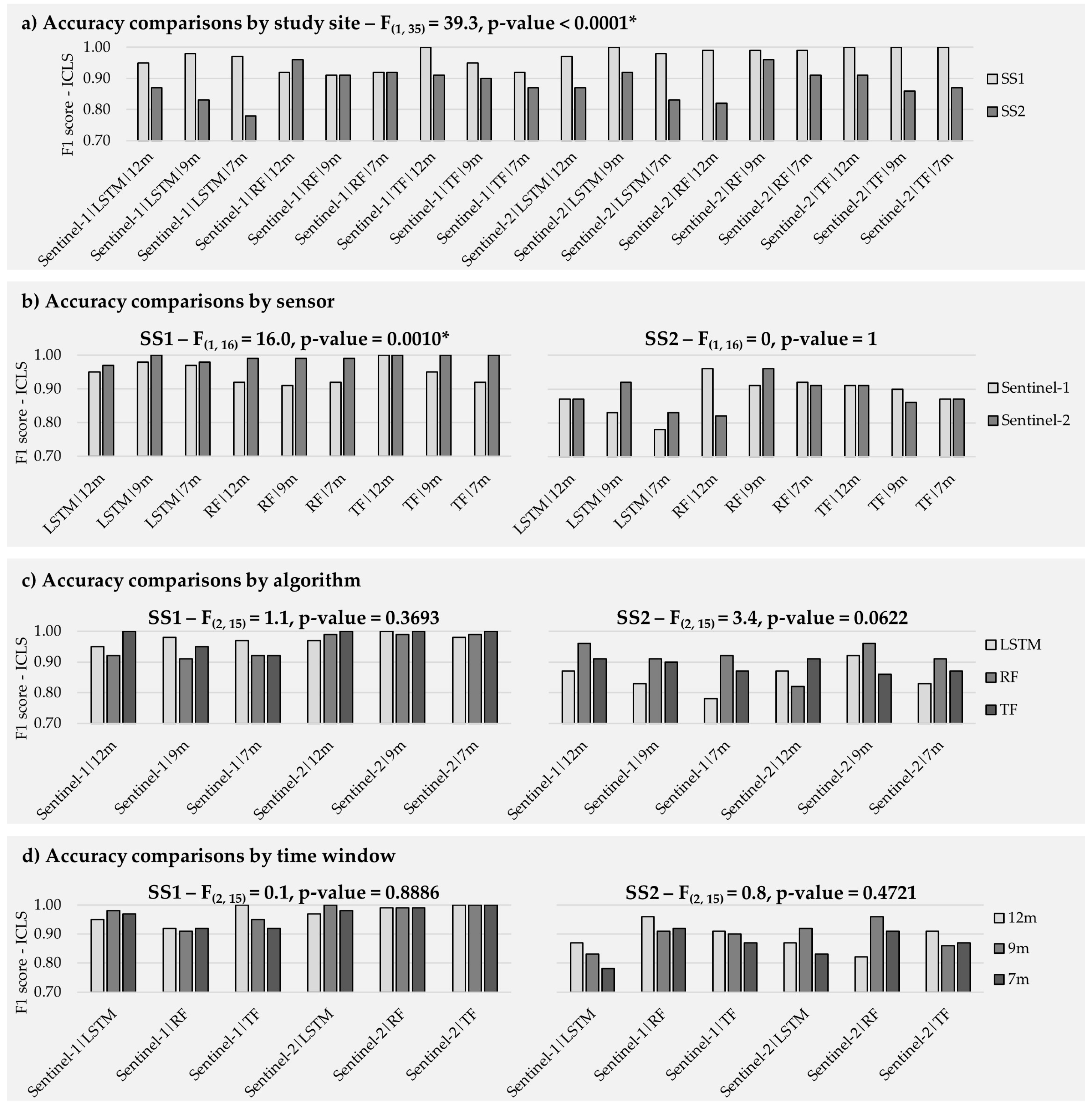
3. Results
3.1. Sensor Accuracy
3.2. Algorithm Accuracy
3.3. Early Season
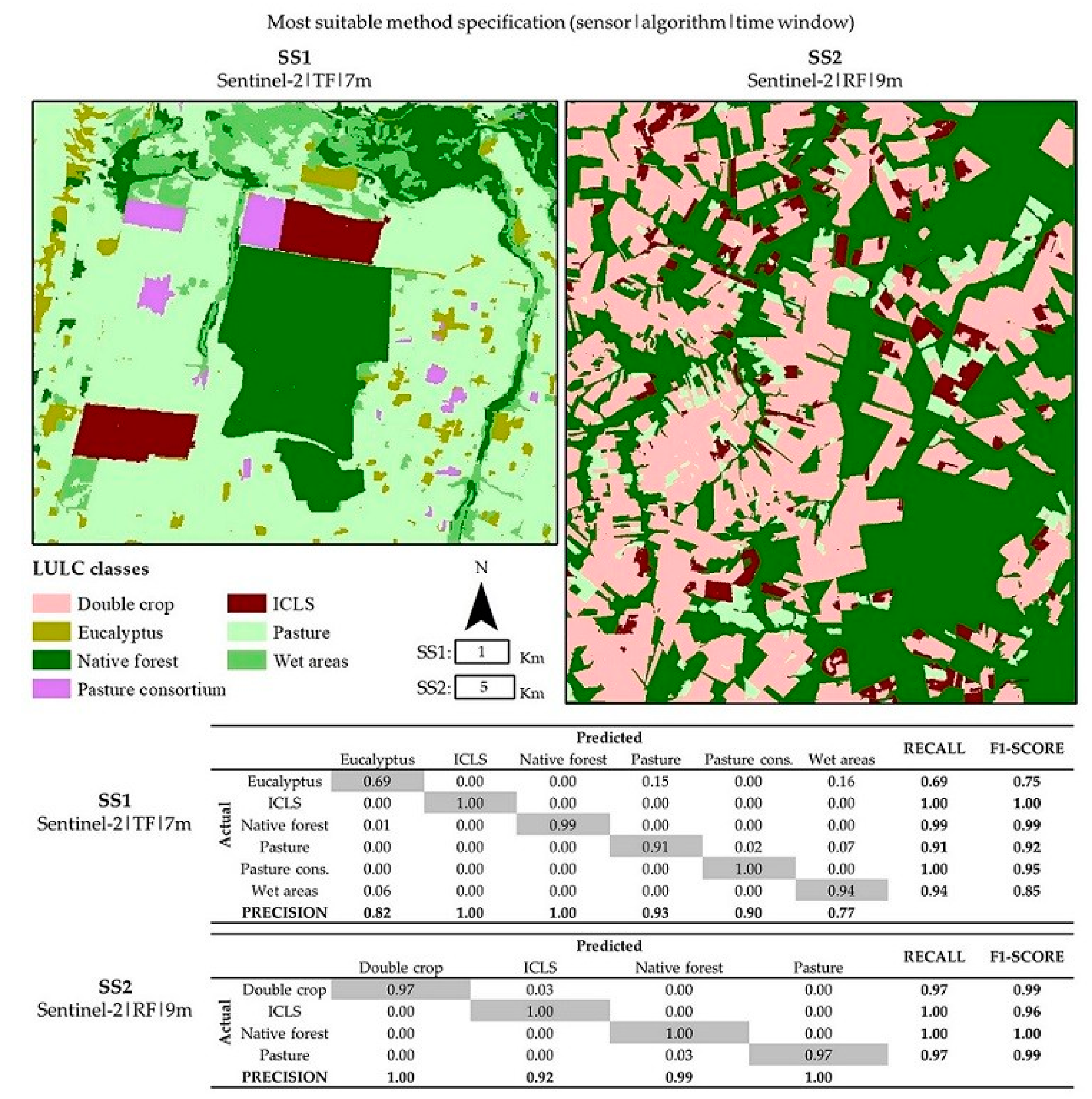
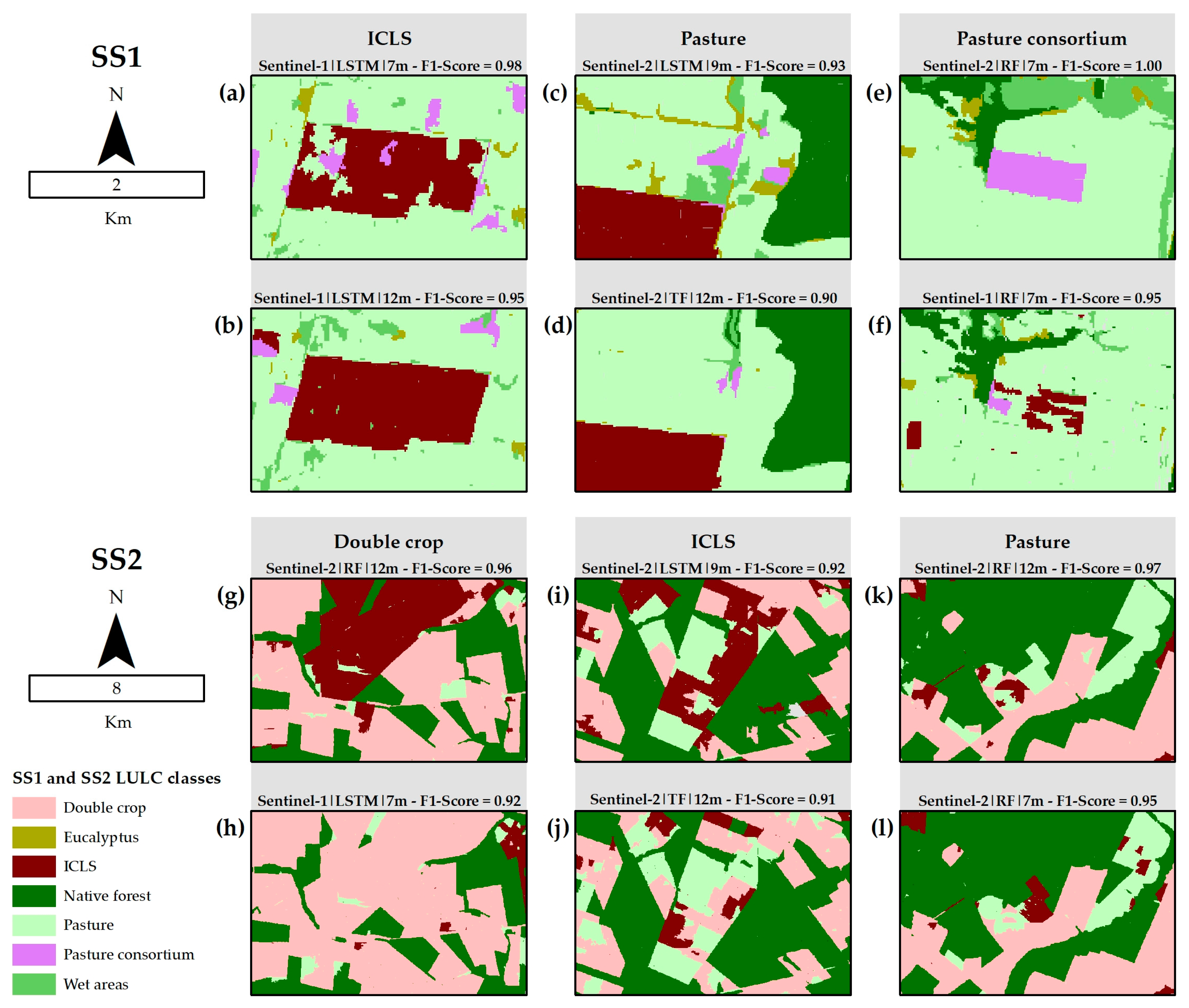
3.4. Predictions
4. Discussion
5. Conclusions
Author Contributions
Funding
Acknowledgments
Conflicts of Interest
References
- Toensmeier, E. The Carbon Farming Solution: A Global Toolkit of Perennial Crops and Regenerative Agriculture Practices for Climate Change Mitigation and Food Security; Chelsea Green Publishing: Chelsea, VT, USA, 2016. [Google Scholar]
- Cordeiro, L.; Kluthcouski, J.; Silva, J.; Rojas, D.; Omote, H.; Moro, E.; Silva, P.; Tiritan, C.; Longen, A. Integração Lavoura-Pecuária em Solos Arenosos: Estudo de Caso da Fazenda Campina no Oeste Paulista; Embrapa Cerrados-Doc. (INFOTECA-E): Planaltina, Brasil, 2020. [Google Scholar]
- Giller, K.E.; Hijbeek, R.; Andersson, J.A.; Sumberg, J. Regenerative agriculture: An agronomic perspective. Outlook Agric. 2021, 50, 13–25. [Google Scholar] [CrossRef]
- Gennari, P.; Rosero-Moncayo, J.; Tubiello, F.N. The FAO contribution to monitoring SDGs for food and agriculture. Nat. Plants 2019, 5, 1196–1197. [Google Scholar] [CrossRef]
- Dos Reis, A.A.; Werner, J.P.; Silva, B.C.; Figueiredo, G.K.; Antunes, J.F.; Esquerdo, J.C.; Coutinho, A.C.; Lamparelli, R.A.; Rocha, J.V.; Magalhães, P.S. Monitoring pasture aboveground biomass and canopy height in an integrated crop–livestock system using textural information from PlanetScope imagery. Remote Sens. 2020, 12, 2534. [Google Scholar] [CrossRef]
- Weiss, M.; Jacob, F.; Duveiller, G. Remote sensing for agricultural applications: A meta-review. Remote Sens. Environ. 2020, 236, 111402. [Google Scholar] [CrossRef]
- Kuchler, P.C.; Simões, M.; Ferraz, R.; Arvor, D.; de Almeida Machado, P.L.O.; Rosa, M.; Gaetano, R.; Bégué, A. Monitoring Complex Integrated Crop–Livestock Systems at Regional Scale in Brazil: A Big Earth Observation Data Approach. Remote Sens. 2022, 14, 1648. [Google Scholar] [CrossRef]
- Almeida, H.S.; Dos Reis, A.A.; Werner, J.P.; Antunes, J.F.; Zhong, L.; Figueiredo, G.K.; Esquerdo, J.C.; Coutinho, A.C.; Lamparelli, R.A.; Magalhães, P.S. Deep Neural Networks for Mapping Integrated Crop-Livestock Systems Using Planetscope Time Series. In Proceedings of the 2021 IEEE International Geoscience and Remote Sensing Symposium IGARSS, Brussels, Belgium, 11–16 July 2021; pp. 4224–4227. [Google Scholar]
- Manabe, V.D.; Melo, M.R.; Rocha, J.V. Framework for mapping integrated crop-livestock systems in Mato Grosso, Brazil. Remote Sens. 2018, 10, 1322. [Google Scholar] [CrossRef] [Green Version]
- Zhang, H.; Kang, J.; Xu, X.; Zhang, L. Accessing the temporal and spectral features in crop type mapping using multi-temporal Sentinel-2 imagery: A case study of Yi’an County, Heilongjiang province, China. Comput. Electron. Agric. 2020, 176, 105618. [Google Scholar] [CrossRef]
- Zhao, H.; Duan, S.; Liu, J.; Sun, L.; Reymondin, L. Evaluation of Five Deep Learning Models for Crop Type Mapping Using Sentinel-2 Time Series Images with Missing Information. Remote Sens. 2021, 13, 2790. [Google Scholar] [CrossRef]
- Sarvia, F.; Xausa, E.; Petris, S.D.; Cantamessa, G.; Borgogno-Mondino, E. A Possible Role of Copernicus Sentinel-2 Data to Support Common Agricultural Policy Controls in Agriculture. Agronomy 2021, 11, 110. [Google Scholar] [CrossRef]
- Wang, J.; Xiao, X.; Bajgain, R.; Starks, P.; Steiner, J.; Doughty, R.B.; Chang, Q. Estimating leaf area index and aboveground biomass of grazing pastures using Sentinel-1, Sentinel-2 and Landsat images. ISPRS J. Photogramm. Remote Sens. 2019, 154, 189–201. [Google Scholar] [CrossRef] [Green Version]
- Lambert, M.J.; Traoré, P.C.S.; Blaes, X.; Baret, P.; Defourny, P. Estimating smallholder crops production at village level from Sentinel-2 time series in Mali’s cotton belt. Remote Sens. Environ. 2018, 216, 647–657. [Google Scholar] [CrossRef]
- Eckardt, R.; Berger, C.; Thiel, C.; Schmullius, C. Removal of optically thick clouds from multi-spectral satellite images using multi-frequency SAR data. Remote Sens. 2013, 5, 2973–3006. [Google Scholar] [CrossRef] [Green Version]
- Alonso, J.; Vaidyanathan, K.; Pietrantuono, R. SAR Handbook Chapter: Measurements-based aging analysis. In Proceedings of the 2020 IEEE International Symposium on Software Reliability Engineering Workshops (ISSREW), Coimbra, Portugal, 12–15 October 2020; pp. 323–324. [Google Scholar]
- Liu, C.A.; Chen, Z.X.; Yun, S.; Chen, J.S.; Hasi, T.; Pan, H.Z. Research advances of SAR remote sensing for agriculture applications: A review. J. Integr. Agric. 2019, 18, 506–525. [Google Scholar] [CrossRef] [Green Version]
- Gella, G.W.; Bijker, W.; Belgiu, M. Mapping crop types in complex farming areas using SAR imagery with dynamic time warping. ISPRS J. Photogramm. Remote Sens. 2021, 175, 171–183. [Google Scholar] [CrossRef]
- Solano-Correa, Y.T.; Bovolo, F.; Bruzzone, L.; Fernández-Prieto, D. Spatio-temporal evolution of crop fields in Sentinel-2 Satellite Image Time Series. In Proceedings of the 2017 9th International Workshop on the Analysis of Multitemporal Remote Sensing Images (MultiTemp), Brugge, Belgium, 27–29 June 2017; pp. 1–4. [Google Scholar]
- Tian, H.; Wang, Y.; Chen, T.; Zhang, L.; Qin, Y. Early-Season Mapping of Winter Crops Using Sentinel-2 Optical Imagery. Remote Sens. 2021, 13, 3822. [Google Scholar] [CrossRef]
- Zhang, H.; Du, H.; Zhang, C.; Zhang, L. An automated early-season method to map winter wheat using time-series Sentinel-2 data: A case study of Shandong, China. Comput. Electron. Agric. 2021, 182, 105962. [Google Scholar] [CrossRef]
- Charvat, K.; Horakova, S.; Druml, S.; Mayer, W.; Safar, V.; Kubickova, H.; Catucci, A. D5. 6 White Paper on Earth Observation Data in Agriculture; Deliverable of the EO4Agri Project, Grant Agreement 821940 (2020).
- Zhong, L.; Hu, L.; Yu, L.; Gong, P.; Biging, G.S. Automated mapping of soybean and corn using phenology. ISPRS J. Photogramm. Remote Sens. 2016, 119, 151–164. [Google Scholar] [CrossRef] [Green Version]
- Fontanelli, G.; Lapini, A.; Santurri, L.; Pettinato, S.; Santi, E.; Ramat, G.; Pilia, S.; Baroni, F.; Tapete, D.; Cigna, F.; et al. Early-Season Crop Mapping on an Agricultural Area in Italy Using X-Band Dual-Polarization SAR Satellite Data and Convolutional Neural Networks. IEEE J. Sel. Top. Appl. Earth Obs. Remote Sens. 2022, 15, 6789–6803. [Google Scholar] [CrossRef]
- Hao, P.-Y.; Tang, H.-J.; Chen, Z.-X.; Meng, Q.-Y.; Kang, Y.-P. Early-season crop type mapping using 30-m reference time series. J. Integr. Agric. 2020, 19, 1897–1911. [Google Scholar] [CrossRef]
- Forkuor, G.; Conrad, C.; Thiel, M.; Ullmann, T.; Zoungrana, E. Integration of optical and Synthetic Aperture Radar imagery for improving crop mapping in Northwestern Benin, West Africa. Remote Sens. 2014, 6, 6472–6499. [Google Scholar] [CrossRef] [Green Version]
- Campos-Taberner, M.; García-Haro, F.J.; Martínez, B.; Sánchez-Ruíz, S.; Gilabert, M.A. A copernicus sentinel-1 and sentinel-2 classification framework for the 2020+ European common agricultural policy: A case study in València (Spain). Agronomy 2019, 9, 556. [Google Scholar] [CrossRef] [Green Version]
- Ma, L.; Liu, Y.; Zhang, X.; Ye, Y.; Yin, G.; Johnson, B.A. Deep learning in remote sensing applications: A meta-analysis and review. ISPRS J. Photogramm. Remote Sens. 2019, 152, 166–177. [Google Scholar] [CrossRef]
- Vaswani, A.; Shazeer, N.; Parmar, N.; Uszkoreit, J.; Jones, L.; Gomez, A.N.; Kaiser, Ł. Polosukhin, Attention is all you need. In Proceedings of the Advances in Neural Information Processing Systems, Long Beach, CA, USA, 4–9 December 2017; pp. 5998–6008. [Google Scholar]
- Rußwurm, M.; Körner, M. Self-attention for raw optical satellite time series classification. ISPRS J. Photogramm. Remote Sens. 2020, 169, 421–435. [Google Scholar] [CrossRef]
- Garnot, V.S.F.; Landrieu, L.; Giordano, S.; Chehata, N. Satellite image time series classification with pixel-set encoders and temporal self-attention. In Proceedings of the Proceedings of the IEEE/CVF Conference on Computer Vision and Pattern Recognition, Seattle, WA, USA, 13–19 June 2020; pp. 12325–12334. [Google Scholar]
- Ofori-Ampofo, S.; Pelletier, C.; Lang, S. Crop type mapping from optical and radar time series using attention-based deep learning. Remote Sens. 2021, 13, 4668. [Google Scholar] [CrossRef]
- Obadic, I.; Roscher, R.; Oliveira, D.A.B.; Zhu, X.X. Exploring Self-Attention for Crop-type Classification Explainability. arXiv 2022, arXiv:2210.13167. [Google Scholar]
- Moraine, M.; Duru, M.; Nicholas, P.; Leterme, P.; Therond, O. Farming system design for innovative crop-livestock integration in Europe. Animal 2014, 8, 1204–1217. [Google Scholar] [CrossRef] [Green Version]
- Balbino, L.C.; Barcellos, A.O.; Stone, L.F. Marco Referencial: Integração Lavoura-Pecuária-Floresta; Embrapa: Brasília, Brazil, 2011; 130p. [Google Scholar]
- Cortner, O.; Garrett, R.D.; Valentim, J.F.; Ferreira, J.; Niles, M.T.; Reis, J.; Gil, J. Perceptions of integrated crop-livestock systems for sustainable intensification in the Brazilian Amazon. Land Use Policy 2019, 82, 841–853. [Google Scholar] [CrossRef]
- Alvares, C.A.; Stape, J.L.; Sentelhas, P.C.; Gonçalves, J.d.M.; Sparovek, G. Köppen’s climate classification map for Brazil. Meteorol. Z. 2013, 22, 711–728. [Google Scholar] [CrossRef]
- Skorupa, L.A.C.V.; Manzatto, C.N.P.M.A. LADISLAU ARAUJO SKORUPA, and CELSO VAINER MANZATTO. In Sistemas de Integração Lavoura-Pecuária-Floresta no Brasil: Estratégias Regionais de Transferência de Tecnologia, Avaliação da Adoção e de Impactos; Embrapa: Brasília, Brazil, 2019; pp. 65–104. [Google Scholar]
- CONAB-Calendario Agrícola Kernel Description. Available online: https://www.conab.gov.br/institucional/publicacoes/outras-publicacoes/item/7694-calendario-agricola-plantio-e-colheita (accessed on 30 January 2022).
- De Keukelaere, L.; Sterckx, S.; Adriaensen, S.; Knaeps, E.; Reusen, I.; Giardino, C.; Bresciani, M.; Hunter, P.; Neil, C.; van der Zande, D.; et al. Atmospheric correction of Landsat-8/OLI and Sentinel-2/MSI data using iCOR algorithm: Validation for coastal and inland waters. Eur. J. Remote Sens. 2018, 51, 525–542. [Google Scholar] [CrossRef] [Green Version]
- Xue, J.; Su, B. Significant remote sensing vegetation indices: A review of developments and applications. J. Sens. 2017, 2017, 1353691. [Google Scholar] [CrossRef] [Green Version]
- Li, T.; Wang, Y.; Liu, C.; Tu, S. Research on identification of multiple cropping index of farmland and regional optimization scheme in China based on NDVI data. Land 2021, 10, 861. [Google Scholar] [CrossRef]
- Holtgrave, A.K.; Röder, N.; Ackermann, A.; Erasmi, S.; Kleinschmit, B. Comparing Sentinel-1 and-2 data and indices for agricultural land use monitoring. Remote Sens. 2020, 12, 2919. [Google Scholar] [CrossRef]
- Rouse, J.W.; Haas, R.H.; Schell, J.A.; Deering, D.W. Monitoring vegetation systems in the Great Plains with ERTS. NASA Spec. Publ. 1974, 351, 309. [Google Scholar]
- Gitelson, A.; Merzlyak, M.N. Spectral reflectance changes associated with autumn senescence of Aesculus hippocastanum Land Acer platanoides L. leaves. Spectral features and relation to chlorophyll estimation. J. Plant Physiol. 1994, 143, 286–292. [Google Scholar]
- Liu, H.Q.; Huete, A. A feedback based modification of the NDVI to minimize canopy back-ground and atmospheric noise. IEEE Trans. Geosci. Remote Sens. 1995, 33, 457–465. [Google Scholar] [CrossRef]
- Cloutis, E.; Connery, D.; Major, D.; Dover, F. Airborne multi-spectral monitoring of agricultural crop status: Effect of time of year, crop type and crop condition parameter. Remote Sens. 1996, 17, 2579–2601. [Google Scholar] [CrossRef]
- Dey, S. Radar Vegetation Index Code for Dual Polarimetric Sentinel-1 Data in EO Browser. Available online: https://custom-scripts.sentinel-hub.com/custom-scripts/sentinel-1/radar_vegetation_index_code_dual_polarimetric/supplementary_material.pdf. (accessed on 3 June 2022).
- Vreugdenhil, M.; Wagner, W.; Bauer-Marschallinger, B.; Pfeil, I.; Teubner, I.; Rüdiger, C.; Strauss, P. Sensitivity of Sentinel-1 backscatter to vegetation dynamics: An Austrian case study. Remote Sens. 2018, 10, 1396. [Google Scholar] [CrossRef] [Green Version]
- Achanta, R.; Susstrunk, S. Superpixels and polygons using simple non-iterative clustering. In Proceedings of the IEEE Conference on Computer Vision and Pattern Recognition, Honolulu, HI, USA, 21–26 July 2017; pp. 4651–4660. [Google Scholar]
- Gorelick, N.; Hancher, M.; Dixon, M.; Ilyushchenko, S.; Thau, D.; Moore, R. Google Earth Engine: Planetary-scale geospatial analysis for everyone. Remote Sens. Environ. 2017, 202, 18–27. [Google Scholar] [CrossRef]
- Ren, X.; Malik, J. Learning a classification model for segmentation. In Proceedings of the Computer Vision, IEEE International Conference on IEEE Computer Society, Nice, France, 13–16 October 2003; Volume 2, p. 10. [Google Scholar]
- Dos Santos, L.; Werner, J.; Dos Reis, A.; Toro, A.; Antunes, J.; Coutinho, A.; Lamparelli, R.; Magalhães, P.; Esquerdo, J.; Figueiredo, G. Multitemporal segmentation of sentinel-2 images in an agricultural intensification region in brazil. ISPRS Ann. Photogramm. Remote Sens. Spat. Inf. Sci. 2022, 3, 389–395. [Google Scholar] [CrossRef]
- Immitzer, M.; Atzberger, C.; Koukal, T. Tree species classification with random forest using very high spatial resolution 8-band WorldView-2 satellite data. Remote Sens. 2012, 4, 2661–2693. [Google Scholar] [CrossRef] [Green Version]
- Belgiu, M.; Csillik, O. Sentinel-2 cropland mapping using pixel-based and object-based time- weighted dynamic time warping analysis. Remote Sens. Environ. 2018, 204, 509–523. [Google Scholar] [CrossRef]
- Meyer, H.; Kühnlein, M.; Appelhans, T.; Nauss, T. Comparison of four machine learning algorithms for their applicability in satellite-based optical rainfall retrievals. Atmos. Res. 2016, 169, 424–433. [Google Scholar] [CrossRef]
- Saini, R.; Ghosh, S. Crop classification on single date sentinel-2 imagery using random forest and suppor vector machine. Int. Arch. Photogramm. Remote Sens. Spat. Inf. Sci. 2018, XLII-5, 683–688. [Google Scholar]
- Khosravi, I.; Alavipanah, S.K. A random forest-based framework for crop mapping using temporal, spectral, textural and polarimetric observations. Int. J. Remote Sens. 2019, 40, 7221–7251. [Google Scholar] [CrossRef]
- Hochreiter, S.; Schmidhuber, J. LSTM can solve hard long time lag problems. In Proceedings of the Advances in Neural Information Processing Systems 9 (NIPS 1996), Denver, CO, USA, 2–5 December 1996; pp. 473–479. [Google Scholar]
- Xia, J.; Falco, N.; Benediktsson, J.A.; Du, P.; Chanussot, J. Hyperspectral image classification with rotation random forest via KPCA. IEEE J. Sel. Top. Appl. Earth Obs. Remote Sens. 2017, 10, 1601–1609. [Google Scholar] [CrossRef] [Green Version]
- Ahmed, M.; Samee, M.R.; Mercer, R.E. Improving tree-LSTM with tree attention. In Proceedings of the 2019 IEEE 13th International Conference on Semantic Computing (ICSC), Newport Beach, CA, USA, 30 January–1 February 2019; pp. 247–254. [Google Scholar]
- Géron, A. Hands-on Machine Learning with Scikit-Learn, Keras, and TensorFlow: Concepts, Tools, and Techniques to Build Intelligent Systems; O’Reilly Media: Sebastopol, CA, USA, 2019. [Google Scholar]
- Goodfellow, I.; Bengio, Y.; Courville, A. Deep Learning; MIT Press: Cambridge, MA, USA, 2016. [Google Scholar]
- Zhao, H.; Chen, Z.; Jiang, H.; Jing, W.; Sun, L.; Feng, M. Evaluation of three deep learning models for early crop classification using sentinel-1A imagery time series—A case study in Zhanjiang, China. Remote Sens. 2019, 11, 2673. [Google Scholar] [CrossRef] [Green Version]
- Dai, Z.; Yang, Z.; Yang, Y.; Carbonell, J.; Le, Q.V.; Salakhutdinov, R. Transformer-xl: Attentive language models beyond a fixed-length context. arXiv 2019, arXiv:1901.02860. [Google Scholar]
- Rußwurm, M.; Lefèvre, S.; Körner, M. Breizhcrops: A satellite time series dataset for crop type identification. In Proceedings of the International Conference on Machine Learning Time Series Workshop, Long Beach, CA, USA, 10–15 June 2019; Volume 3. [Google Scholar]
- Voita, E.; Talbot, D.; Moiseev, F.; Sennrich, R.; Titov, I. Analyzing multi-head self-attention: Specialized heads do the heavy lifting, the rest can be pruned. arXiv 2019, arXiv:1905.09418. [Google Scholar]
- Wang, J.; Xu, M.; Wang, H.; Zhang, J. Classification of imbalanced data by using the SMOTE algorithm and locally linear embedding. In Proceedings of the 8th International Conference on Signal Processing, Guilin, China, 16–20 November 2006; Volume 3. [Google Scholar]
- Tiku, M. Tables of the power of the F-test. J. Am. Stat. Assoc. 1967, 62, 525–539. [Google Scholar] [CrossRef]
- Thiese, M.S.; Ronna, B.; Ott, U. P value interpretations and considerations. J. Thorac. Dis. 2016, 8, E928. [Google Scholar] [CrossRef] [PubMed] [Green Version]
- Pearson, E.S.; Hartley, H.O. Charts of the power function for analysis of variance tests, derived from the non-central F-distribution. Biometrika 1951, 38, 112–130. [Google Scholar] [CrossRef] [PubMed]
- Kuemmerle, T.; Erb, K.; Meyfroidt, P.; Müller, D.; Verburg, P.H.; Estel, S.; Haberl, H.; Hostert, P.; Jepsen, M.R.; Kastner, T.; et al. Challenges and opportunities in mapping land use intensity globally. Curr. Opin. Environ. Sustain. 2013, 5, 484–493. [Google Scholar] [CrossRef] [PubMed]
- Nyborg, J.; Pelletier, C.; Lefèvre, S.; Assent, I. TimeMatch: Unsupervised cross-region adaptation by temporal shift estimation. ISPRS J. Photogramm. Remote Sens. 2022, 188, 301–313. [Google Scholar] [CrossRef]
- Sun, C.; Bian, Y.; Zhou, T.; Pan, J. Using of multi-source and multi-temporal remote sensing data improves crop-type mapping in the subtropical agriculture region. Sensors 2019, 19, 2401. [Google Scholar] [CrossRef] [PubMed] [Green Version]
- Misra, G.; Cawkwell, F.; Wingler, A. Status of phenological research using Sentinel-2 data: A review. Remote Sens. 2020, 12, 2760. [Google Scholar] [CrossRef]
- Phiri, D.; Simwanda, M.; Salekin, S.; Nyirenda, V.R.; Murayama, Y.; Ranagalage, M. Sentinel-2 data for land cover/use mapping: A review. Remote Sens. 2020, 12, 2291. [Google Scholar] [CrossRef]
- Qu, Y.; Zhao, W.; Yuan, Z.; Chen, J. Crop mapping from sentinel-1 polarimetric time-series with a deep neural network. Remote Sens. 2020, 12, 2493. [Google Scholar] [CrossRef]
- Mestre-Quereda, A.; Lopez-Sanchez, J.M.; Vicente-Guijalba, F.; Jacob, A.W.; Engdahl, M.E. Time-series of Sentinel-1 interferometric coherence and backscatter for crop-type mapping. IEEE J. Sel. Top. Appl. Earth Obs. Remote Sens. 2020, 13, 4070–4084. [Google Scholar] [CrossRef]
- Guo, Z.; Qi, W.; Huang, Y.; Zhao, J.; Yang, H.; Koo, V.C.; Li, N. Identification of Crop Type Based on C-AENN Using Time Series Sentinel-1A SAR Data. Remote Sens. 2022, 14, 1379. [Google Scholar] [CrossRef]
- Veloso, A.; Mermoz, S.; Bouvet, A.; Le Toan, T.; Planells, M.; Dejoux, J.F.; Ceschia, E. Understanding the temporal behavior of crops using Sentinel-1 and Sentinel-2-like data for agricultural applications. Remote Sens. Environ. 2017, 199, 415–426. [Google Scholar] [CrossRef]
- Asam, S.; Gessner, U.; Almengor González, R.; Wenzl, M.; Kriese, J.; Kuenzer, C. Mapping Crop Types of Germany by Combining Temporal Statistical Metrics of Sentinel-1 and Sentinel-2 Time Series with LPIS Data. Remote Sens. 2022, 14, 2981. [Google Scholar] [CrossRef]
- Adrian, J.; Sagan, V.; Maimaitijiang, M. Sentinel SAR-optical fusion for crop type mapping using deep learning and Google Earth Engine. ISPRS J. Photogramm. Remote Sens. 2021, 175, 215–235. [Google Scholar] [CrossRef]
- Reuß, F.; Greimeister-Pfeil, I.; Vreugdenhil, M.; Wagner, W. Comparison of Long Short-Term Memory Networks and Random Forest for Sentinel-1 Time Series Based Large Scale Crop Classification. Remote Sens. 2021, 13, 5000. [Google Scholar] [CrossRef]
- Ge, S.; Zhang, J.; Pan, Y.; Yang, Z.; Zhu, S. Transferable deep learning model based on the phenological matching principle for mapping crop extent. Int. J. Appl. Earth Obs. Geoinf. 2021, 102, 102451. [Google Scholar] [CrossRef]
- Fritz, S.; See, L.; Bayas, J.C.L.; Waldner, F.; Jacques, D.; Becker-Reshef, I.; Whitcraft, A.; Baruth, B.; Bonifacio, R.; Crutchfield, J.; et al. A comparison of global agricultural monitoring systems and current gaps. Agric. Syst. 2019, 168, 258–272. [Google Scholar] [CrossRef]


| Sensor | Index | Equation | Reference |
|---|---|---|---|
| Sentinel-2 | Normalized Difference Vegetation Index—NDVI |
(NIR − RED)/(NIR + RED) (NIR − REDEDGE)/(NIR + REDEDGE) (2.5 × NIR − RED)/(NIR + 6RED − 7.5BLUE) + 1) (REDEDGE/RED) (VH × 4)/(VH + VV) VH/VV | [44] |
| Sentinel-2 | Normalized Difference Red Edge Index—NDRE | [45] | |
| Sentinel-2 | Enhanced Vegetation Index—EVI | [46] | |
| Sentinel-2 | RED EDGE 1 | [47] | |
| Sentinel-1 | Radar Vegetation Index—RVI | [48] | |
| Sentinel-1 | VH and VV ratio | [49] |
| Study Site | Algorithm | Sensor | Time Window | F1 Score—Overall | Precision—ICLS | Recall—ICLS | F1 Score—ICLS |
|---|---|---|---|---|---|---|---|
| RF | Sentinel—1 | Entire Season | 0.87 | 0.92 | 0.92 | 0.92 | |
| RF | Sentinel—1 | Sep–Jun | 0.86 | 0.94 | 0.87 | 0.91 | |
| RF | Sentinel—1 | Sep–Apr | 0.87 | 0.9 | 0.95 | 0.92 | |
| RF | Sentinel—2 | Entire Season | 0.98 | 1.00 | 0.98 | 0.99 | |
| RF | Sentinel—2 | Sep–Jun | 0.98 | 1.00 | 0.98 | 0.99 | |
| RF | Sentinel—2 | Sep–Apr | 0.97 | 1.00 | 0.98 | 0.99 | |
| LSTM | Sentinel—1 | Entire Season | 0.89 | 0.97 | 0.94 | 0.95 | |
| LSTM | Sentinel—1 | Sep–Jun | 0.88 | 1.00 | 0.97 | 0.98 | |
| SS1 | LSTM LSTM | Sentinel—1 Sentinel—2 | Sep–Apr Entire Season | 0.89 0.96 | 0.97 0.94 | 0.97 1.00 | 0.97 0.97 |
| LSTM | Sentinel—2 | Sep–Jun | 0.97 | 1.00 | 1.00 | 1.00 | |
| LSTM | Sentinel—2 | Sep–Apr | 0.95 | 0.97 | 1.00 | 0.98 | |
| TF | Sentinel—1 | Entire Season | 0.86 | 1.00 | 1.00 | 1.00 | |
| TF | Sentinel—1 | Sep–Jun | 0.85 | 0.97 | 0.94 | 0.95 | |
| TF | Sentinel—1 | Sep–Apr | 0.86 | 0.96 | 0.87 | 0.92 | |
| TF | Sentinel—2 | Entire Season | 0.96 | 1.00 | 1.00 | 1.00 | |
| TF | Sentinel—2 | Sep–Jun | 0.97 | 1.00 | 1.00 | 1.00 | |
| TF | Sentinel—2 | Sep–Apr | 0.95 | 1.00 | 1.00 | 1.00 | |
| RF | Sentinel—1 | Entire Season | 1.00 | 1.00 | 0.92 | 0.96 | |
| RF | Sentinel—1 | Sep–Jun | 0.99 | 1.00 | 0.83 | 0.91 | |
| RF | Sentinel—1 | Sep–Apr | 0.99 | 0.92 | 0.92 | 0.92 | |
| RF | Sentinel—2 | Entire Season | 0.98 | 0.9 | 0.75 | 0.82 | |
| RF | Sentinel—2 | Sep–Jun | 0.99 | 0.92 | 1.00 | 0.96 | |
| RF | Sentinel—2 | Sep–Apr | 0.99 | 1.00 | 0.83 | 0.91 | |
| LSTM | Sentinel—1 | Entire Season | 0.99 | 0.91 | 0.83 | 0.87 | |
| LSTM | Sentinel—1 | Sep–Jun | 0.98 | 0.83 | 0.83 | 0.83 | |
| SS2 | LSTM LSTM | Sentinel—1 Sentinel—2 | Sep–Apr Entire Season | 0.98 0.98 | 0.82 0.91 | 0.75 0.83 | 0.78 0.87 |
| LSTM | Sentinel—2 | Sep–Jun | 0.99 | 0.92 | 0.92 | 0.92 | |
| LSTM | Sentinel—2 | Sep–Apr | 0.97 | 0.83 | 0.83 | 0.83 | |
| TF | Sentinel—1 | Entire Season | 0.97 | 1.00 | 0.83 | 0.91 | |
| TF | Sentinel—1 | Sep–Jun | 0.98 | 1.00 | 0.83 | 0.90 | |
| TF | Sentinel—1 | Sep–Apr | 0.97 | 0.91 | 0.83 | 0.87 | |
| TF | Sentinel—2 | Entire Season | 0.97 | 1.00 | 0.83 | 0.91 | |
| TF | Sentinel—2 | Sep–Jun | 0.97 | 1.00 | 0.75 | 0.86 | |
| TF | Sentinel—2 | Sep–Apr | 0.96 | 0.91 | 0.83 | 0.87 |
Disclaimer/Publisher’s Note: The statements, opinions and data contained in all publications are solely those of the individual author(s) and contributor(s) and not of MDPI and/or the editor(s). MDPI and/or the editor(s) disclaim responsibility for any injury to people or property resulting from any ideas, methods, instructions or products referred to in the content. |
© 2023 by the authors. Licensee MDPI, Basel, Switzerland. This article is an open access article distributed under the terms and conditions of the Creative Commons Attribution (CC BY) license (https://creativecommons.org/licenses/by/4.0/).
Share and Cite
Toro, A.P.S.G.D.D.; Bueno, I.T.; Werner, J.P.S.; Antunes, J.F.G.; Lamparelli, R.A.C.; Coutinho, A.C.; Esquerdo, J.C.D.M.; Magalhães, P.S.G.; Figueiredo, G.K.D.A. SAR and Optical Data Applied to Early-Season Mapping of Integrated Crop–Livestock Systems Using Deep and Machine Learning Algorithms. Remote Sens. 2023, 15, 1130. https://doi.org/10.3390/rs15041130
Toro APSGDD, Bueno IT, Werner JPS, Antunes JFG, Lamparelli RAC, Coutinho AC, Esquerdo JCDM, Magalhães PSG, Figueiredo GKDA. SAR and Optical Data Applied to Early-Season Mapping of Integrated Crop–Livestock Systems Using Deep and Machine Learning Algorithms. Remote Sensing. 2023; 15(4):1130. https://doi.org/10.3390/rs15041130
Chicago/Turabian StyleToro, Ana P. S. G. D. D., Inacio T. Bueno, João P. S. Werner, João F. G. Antunes, Rubens A. C. Lamparelli, Alexandre C. Coutinho, Júlio C. D. M. Esquerdo, Paulo S. G. Magalhães, and Gleyce K. D. A. Figueiredo. 2023. "SAR and Optical Data Applied to Early-Season Mapping of Integrated Crop–Livestock Systems Using Deep and Machine Learning Algorithms" Remote Sensing 15, no. 4: 1130. https://doi.org/10.3390/rs15041130