1. Introduction
Demands for GNSS devices continue to increase and will continue doing so in decades to come, due to the explosion of smartphone-based navigation [
1] and intelligent transportation construction [
2]. Therefore, realizing accurate positioning in challenging environments using global navigation satellite system (GNSS) devices is a hot debate these days. However, current GNSS receiver techniques cannot easily satisfy next-generation positioning, navigation, and timing (PNT) performance, due to the intrinsic mechanism of GNSS electromagnetic waveforms. For instance, unlike LTE/5G wireless communication signals, having orthogonal frequency division multiple access (OFDMA) and substantial transmission power [
3,
4], GNSS signals are transmitted at the same frequency. Each signal channel is divided through the code division multiple access (CDMA). The GNSS signals are also confronted with severe channel fading over long-distance transmission (approximately 20,000 km for the GNSS satellites operating in the medium Earth orbit). The former is naturally immune to the multipath effect, while the GNSS signals are less capable of resisting these forms of interference in transmission. Due to this, recent research proposed a hybrid optical–wireless network that achieves decimeter-level terrestrial positioning and sub-nanosecond timing, aimed as a supplement to, or even substitute for, the GNSS device in the future commercial market [
5].
Against this background, there are many remaining problems and vast space regarding new GNSS receiver design, especially in challenging cases, and it is urgent to embark on renewing the current commercial receiver architecture. The CDMA signals are sensitive to the non-line-of-sight (NLOS) ray within one chip range, causing big issues in channel estimation. In recent years, super-resolution algorithms (SRAs) emerged in GNSS signal processing to separate line-of-sight (LOS) and NLOS signals into different orthogonal spaces [
6,
7,
8]. Recent work presented a graph Fourier transform (GFT) filter denoising the complex correlator outputs to replace the old GNSS tracking loop, which can be considered a direct way to steer the code phase in challenging cases [
9]. Except for the separation using the state-of-the-art SRAs or the GNSS antenna changes [
10,
11,
12], modeling the superposition signals formed with LOS and NLOS rays is mainstream in the current GNSS community as a means to overcome multipath interference [
13,
14,
15].
Early in the 1990s, research revealed the prominence of GNSS products in overcoming the predicament of tracking accurate Doppler frequency between the user’s end and the satellite—vector delay lock loop (VDLL) [
16]. The vector approach is an intelligent choice to model the LOS Doppler frequency into a more proper shape. The basic idea of this technique is to leverage the user’s navigation estimates to predict the Doppler frequency as compensation for the time of arrival (TOA) estimation in the GNSS baseband processing, providing a more accurate single-point positioning (SPP) solution. The VDLL allows GNSS researchers to optimize baseband signal modeling with information from multiple channels instead of a conservative loop filter algorithm in a single channel. Later, this idea was extended to assist carrier phase modeling, for which it was nominated as a vector phase lock loop (VPLL) [
17]. Improved versions, and more specific experimental results, based on the VPLL techniques, were presented in the ensuing years [
18,
19]. However, the stability and convergence of the VPLL are vulnerable to being destroyed when a biased error in the code phase modeling is not removed (meaning that a multipath effect interferes with the GNSS baseband and its high-precision navigation solutions). The GNSS carrier and code signals are synchronized and significantly interact with each other.
The wireless communication theory indicates that fast fading [
20], such as the multipath effect on carrier signals, causes a modeling error of a maximum of approximately one-fourth of a signal wavelength, e.g., about 5 cm for global positioning system (GPS) L1 signals [
21]. This value is much smaller than the GNSS code phase error. For example, a typical value of the multipath effect on the code signal is commonly at the meter level, which is two orders of the magnitude of the carrier phase [
22]. Partially resorting to this, carrier-aiding is always used in a traditional GNSS baseband to support the code signal estimation [
23]. Similarly, a vector delay/frequency lock loop (VDFLL) was also presented to enhance the code phase tracking by combining the carrier-aiding and the VDLL approaches [
24].
The conventional vector tracking techniques impose an indirect approach to improving the TOA modeling over the code tracking process inside a GNSS receiver. Vector tracking has the potential to enable the baseband to yield a more accurate code Doppler frequency production. Then, the improved code Doppler replicates instantaneous code phases (i.e., TOA modeling) more precisely, contributing to a higher-quality navigation solution. This type of vector receiver can ultimately alleviate harmful interference to LOS signal estimation, especially when the user’s end is moving [
25]. Nevertheless, little efficiency is available in the traditional vector tracking loop once the received LOS and NLOS rays are not well discriminated, in terms of the Doppler frequency feature (i.e., the frequency or Fourier domain). Unfortunately, this is often the case for today’s GNSS users.
The authors’ recent research presented a method to optimize the TOA model in the GNSS tracking process assisted by an absolute position solution, not simply relying on the code frequency error between the baseband signal replica and the mapped code signal prediction from the user’s navigation solution [
26]. More specifically, we took advantage of the high-accuracy positioning solution (more accurate than code-based-only positioning) to improve TOA modeling, aided by the vector tracking technique in the code phase domain, instead of the code frequency domain. By coincidence, a recent paper using the classic SRA, i.e., root MUSIC, was also published aiming to achieve an analogous goal [
6].
An inertial navigation system (INS) can resist high-frequency random noise in the user’s navigation as it works upon autonomous dead reckoning (DR), rather than relying on external information [
27]. Hence, integrating INS has been a prevalent means to rug the GNSS-based navigation system. To date it has attracted much attention in the navigation field to the extent that low-cost INS increases GNSS-based navigation [
28,
29]. However, research space remains in terms of the influence of low-cost INS on GNSS baseband signal processing.
Regarding these discussions, this work proposes an improved version of the authors’ previous research [
26,
30]. More specifically, a low-cost inertial measurement unit (IMU) is deeply integrated into a GNSS vector delay/frequency/phase lock loop (VDFPLL) software-defined radio (SDR). Meanwhile, an extended Kalman filter (EKF) is used to fuse carrier-based positions and INS DR results. Generally, the carrier-based positioning algorithms can include real-time kinematic (RTK) relying on the base station, and precise point positioning (PPP) based on the high-precision model [
31]. Finally, compared to our previous research [
26], the main contributions of this work include the following:
A low-cost IMU is combined with the float RTK solutions via an EKF and integrated navigation solutions are used to improve the GNSS TOA modeling in a code phase domain instead of a frequency/Fourier domain;
An RTK/INS VDFPLL SDR is proposed and developed, wherein RTK solutions and INS dead reckoning results are integrated, and a traditional scalar tracking loop (STL), VDFLL, and VDFPLL are realized and combined;
An approach showing the effectiveness of the INS in enhancing GNSS baseband processing in a static scenario is presented, based on real-world experiments, which little previous research has discussed.
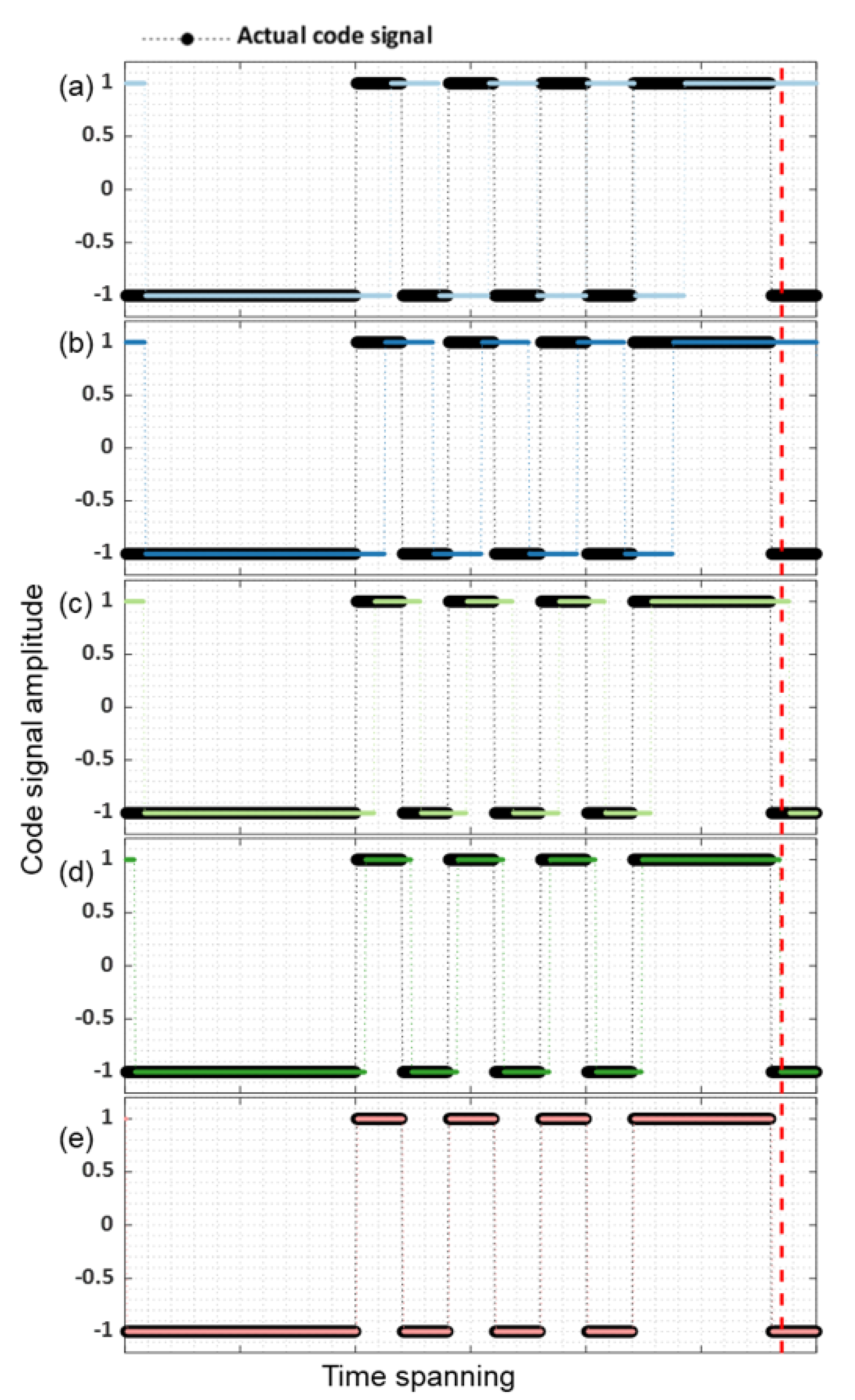
A diagram explaining the difference between the proposed and traditional algorithms towards the code phase estimation in the GNSS baseband is provided in
Figure 1. Before explaining
Figure 1, it is worth emphasizing that the instantaneous code phase error consists of two primary parts regarding standard GNSS baseband processing. They are an absolute one, from the initial code phase error, and a relative one, caused by the Doppler frequency error, in which the received signal subtracts the local replica. These are discussed below.
At first, the conventional STL causes an apparent code Doppler frequency error and initial code phase error (see
Figure 1a) [
23]. Then, the traditional vector tracking compensates for parts of the Doppler frequency error, reducing the relative code phase error (see
Figure 1b) [
16,
32]. Next, the vector tracking technique is further aided by an IMU sensor, so the GNSS baseband becomes more capable of alleviating the frequency error [
33], but the initial code phase error remains (see
Figure 1c). After this, the RTK-based absolute-position-aided (APA) technique is involved in tracking, and the initial code phase error can be reduced (see
Figure 1d) [
26]. Finally, this work proposes a deep integration method of INS and GNSS RTK processing to correct a more absolute code phase error in the local replica (see
Figure 1e).
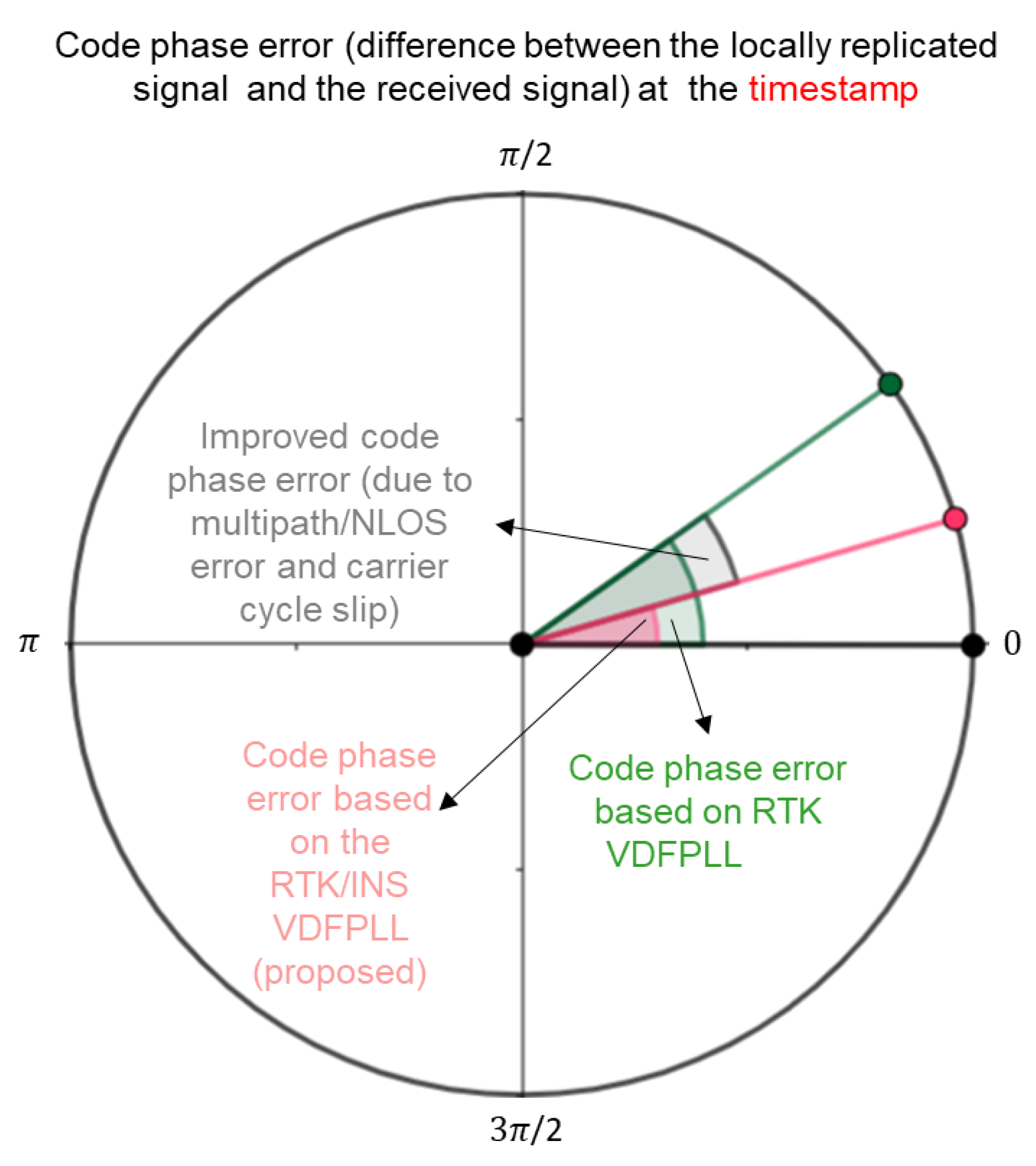
Figure 2 further depicts the code phase errors at the timestamp (see the dashed red lines in
Figure 1) in the tracking process regarding the RTK-only APA and RTK/INS APA techniques. It is worth emphasizing that the timestamp denotes the local clock count to get the TOA estimation in the GNSS baseband (i.e., the time to extract the instantaneous GNSS measurements). Compared to our previous work [
26], the proposed algorithm can improve the code phase estimation by removing the initial code phase error related to the multipath/NLOS effect and the carrier cycle slip (because of the involvement of the RTK-based APA technique). The situation always arises in the real world. For example, the multipath interference in a static GNSS user’s receiver causes such an absolute code phase error issue, which is challenging in the current GNSS community. Therefore, this research derives a method to solve the issue.
The remainder of this paper is organized as follows.
Section 2 introduces the methodology, where the proposed VDFPLL, based on RTK/INS deep integration, is discussed in detail. The RTK-position-aided VDFPLL is briefly introduced. Two real-world stationary experiments are provided and discussed in
Section 3. Finally,
Section 4 concludes this work.
2. Materials and Methods
This section investigates how the APA code phase tracking in a GNSS baseband is realized with the proposed VDFPLL (deeply integrated with the float-RTK positioning and the INS DR). We first recap on the VDFPLL, based on standalone GNSS RTK solutions. Then, its improved form, deeply integrating the INS DR navigation solutions, is discussed. Finally, how the proposed RTK/INS VDFPLL is combined with the STL and the VDFLL in a GPS SDR is elaborated on.
2.1. RTK-Position-Aided VDFPLL
As mentioned earlier, the VDFPLL provides a way to directly steer the local code replica with the user’s absolute position in the code phase domain instead of the conventional code frequency domain. Our previous work achieved this goal by presenting a practical means in the baseband that applies the user’s RTK solution as a source of high-accuracy code phase prediction. This technique is briefly described for the integrity of this work.
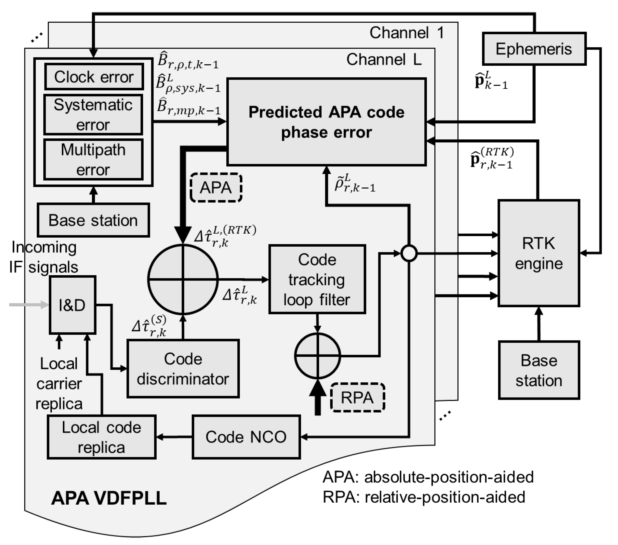
The architecture of the RTK-position-aided VDFPLL is illustrated in
Figure 3, where APA and RPA correspond to absolute- and relative-position-aided, respectively. It is worth noting that the RPA is achieved with the traditional VDFLL technique. The absolute code phase is also tracked, aided by the vector tracking technique in the code phase domain. In this case, the following discriminates the entire code phase error
with
where subscript
k denotes the index of tracking epochs;
is the traditional discriminated code phase error through an early-minus-late-envelope code discriminator;
is the code phase error obtained from the APA approach;
and
are the pseudoranges measured from the code tracking filter and predicted from the float RTK solution, respectively;
is the predicted geometry distance;
is the vector of satellite position;
is the vector of the estimated float RTK position;
is the summation of the local clock bias error estimation and systematic error estimation, computed from base station information and master satellite measurements [
26];
is the estimated multipath delay error imposed on the absolute code phase error via a between-satellite single difference algorithm, and
is its tuned coefficient constant, based on the involved early–late spacing [
30].
Next, the work process of the RTK-position-aided VDFPLL in the GPS SDR within the same tracking epoch is outlined as follows:
Step 1: the SDR receives the incoming intermediate frequency (IF) GPS L1 C/A data via front-end equipment;
Step 2: integration and dumping (I&D) procedures are implemented upon correlators between the local code replica and the incoming IF GPS signals;
Step 3: the correlator output passing through the traditional code discriminator yields ;
Step 4: the bias of the discriminated code error is compensated by the RTK-position-aided (i.e., the APA operation) code error estimation gives ;
Step 5: a code tracking loop filter denoises the code phase error from Step 4;
Step 6: an RPA technique (i.e., the VDFLL) is executed to alleviate the code frequency error in the code-tracking process;
Step 7: a numerically controlled oscillator (NCO) leverages the output of Step 6 to produce the TOA estimation (the raw output of the code loop filter, aided by the Doppler prediction), and the pseudorange measurements (de-noised by the carrier smoothing technique);
Step 8: the RTK engine leverages the pseudoranges and carrier phases (the raw output of the carrier loop filter, aided by the Doppler prediction) from all the tracking channels, navigation data, and the base station information to compute the float RTK solutions;
Step 9: the APA code phase error
is computed with the float-RTK solutions and the pseudorange measurement by (
2);
Step 10: repeating Step 2, the RTK-position-aided VDFPLL works for the next tracking epoch.
To conclude, the work process of the VDFPLL, based on the float-RTK solutions executed in a GNSS SDR is addressed.
2.2. The Proposed VDFPLL Based on RTK/INS Deep Integration
2.2.1. Architectures of the Proposed VDFPLL SDR
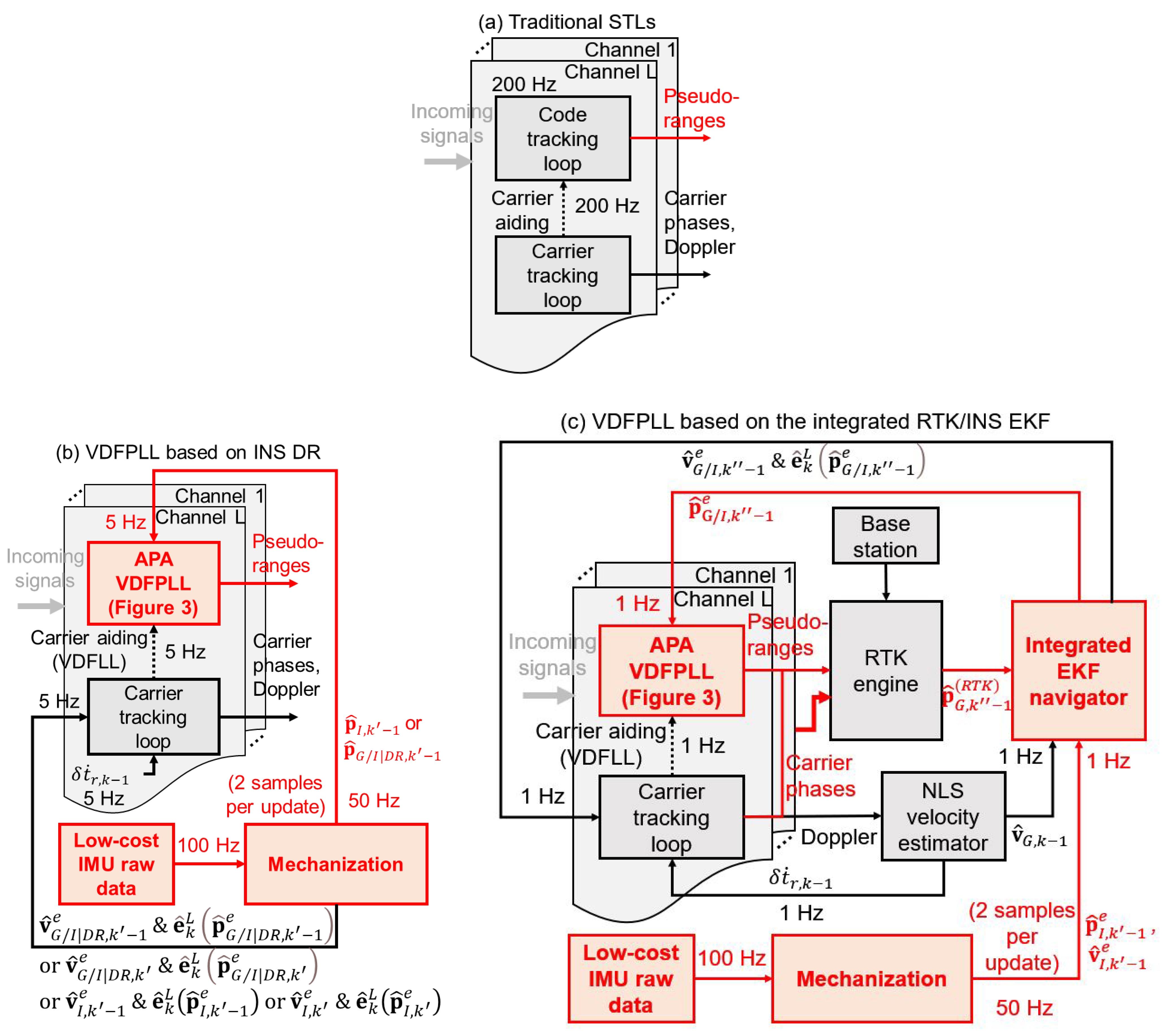
The architectures of the proposed APA VDFPLL GPS SDR deeply integrated with the float RTK solutions and INS dead reckoning results are displayed in
Figure 4. It is worth mentioning that hybrid tracking loops are adopted here due to the data rates discrepancy corresponding to various sources, i.e., the proposed SDR tracking, the base station, and the IMU sensor raw data.
First, there are two procedures for updating the code tracking loop with the APA method in the SDR. On the one hand, the TOA model is predicted from the integrated float RTK/INS EKF, as depicted in
Figure 4c. On the other hand, the proposed VDFPLL updating rate is 5 Hz, which is higher than the RTK solution rate, so the INS DR navigation solutions (with a rate of 50 Hz) are interpolated in the updating process when the RTK solutions (with a rate of 1 Hz) are absent. It is worth noting that we took two samples of the IMU raw data per update to compensate for coning and sculling errors, so the raw data rate of the IMU was 100 Hz, while the DR navigation results were at the rate of 50 Hz.
Finally, as the tracking loop updating rate in the proposed SDR baseband was 200 Hz, much higher than the VDFPLL rate, the traditional STLs for code and carrier tracking were interpolated across the intervals where the VDFPLL was not activated.
As a result, the following three tracking loops jointly work in the proposed RTK/INS-based VDFPLL SDR: the VDFPLL, based on the RTK/INS integrated EKF (see
Figure 4c), the VDFPLL, based on the INS DR (see
Figure 4b), and the traditional STL (see
Figure 4a).
2.2.2. RTK/INS EKF Navigator and INS DR
As illustrated in
Figure 4, three types of TOA estimation are formed in the proposed GNSS SDR, corresponding to
Figure 4a–c, respectively. They are elaborated on below.
In the proposed architecture
Figure 4c, the RTK position solution
is not directly input to the “APA VDFPLL” block as in the architecture in
Figure 3. Instead, this solution is transferred to the EKF navigator integrated with the mechanization results computed from the low-cost IMU raw data. The fusion algorithm of the integrated EKF is explained in detail later. So, the integrated RTK/INS solution output by the EKF engine is finally used to execute the APA VDFPLL algorithm.
At first, the absolute position is estimated from the integrated RTK/INS EKF navigator (see
Figure 4c). The RTK engine comes from an open-source package goGPS v0.4.3 [
34]. Then, the float RTK is deeply integrated into the proposed SDR, introduced in the authors’ previous work [
26]. The SDR platform, to realize the deep integration of RTK and INS, was built and investigated in the authors’ previous publications [
35,
36].
We now discuss the EKF algorithm used in this work. The state transition equation is given by
with
where superscript
e represents the Earth-centered, Earth-fixed (ECEF) coordinate frame; subscript
denotes the epoch index of the EKF updates;
K is the integer ratio of the INS DR and the EKF updating rates, where the former and the latter are 50 Hz and 1 Hz (constrained by the rate of the base station information), respectively;
is the epoch index of INS DR solutions;
M is the integer ratio of the GNSS tracking rate and the INS updating rate where the tracking rate (200 Hz) is no lower than the INS updating rate (50 Hz) here; so it satisfies
;
is the transition matrix;
is the process noise vector. Then, the state vector of the EKF model in the ECEF frame is given by
where
is the attitude error vector;
is the 3D velocity error vector;
is the 3D position error vector;
and
are the respective gyro and accelerometer bias error vectors.
Next, the observation equation is provided as
where
is the observation matrix;
is the observation noise vector. The observation vector, including position errors and velocity errors, is provided as
where
and
correspond to the 3D positions and velocities w.r.t. the ECEF frame, respectively; subscript
I and
G correspond to the solutions obtained from the INS and the GNSS, respectively; the subscript “RTK” means that the GNSS position results are solved by the float RTK algorithm [
26], and the subscript “NLS” represents that the GNSS velocity results are calculated from the standard non-linear least squared (NLS) method [
37]. How to build
and
, as well as how to form the process noise covariance matrix and the observation noise covariance matrix are referred to in [
35].
After the system model was built, the recursive estimation of the EKF algorithm predicts and updates the state vector [
38]. Finally, upon the time epoch, where base station information is available for the RTK algorithm, the navigation solutions corresponding to the velocity, position, and attitude information from the EKF algorithm are given by
where
denotes the skew matrix operator;
is the 3-order identity matrix;
, and
are the estimated state vectors about velocity and position errors, and attitude errors, and
,
and
are the estimated navigation vectors (corresponding to the respective velocity, position, and attitude);
,
and
are the counterparts solely upon the INS DR process, which are introduced later.
Within the epochs where the base station information is missing, the EKF-based results at the previous epoch can contribute to the INS DR process at the current epoch in the following way
with
where
is the updating interval of the EKF;
and
are the specific force and angular rate measurement vectors of the body frame w.r.t. ECEF frame;
is the Earth rotation rate, i.e., 7.292115 ×
10
−5 rad/s and
is its vector form;
is the gravity acceleration vector function in the ECEF frame varying with the user’s position
(see Equations (2.133) and (2.142) in [
27]);
is the Earth rotation matrix from the Earth-centered inertial (ECI) to the ECEF coordinate frame varying with the updating interval
;
isthe averaging transformation matrix w.r.t. the body-to-ECEF-frame coordinate obtained from
(see Equations (5.84) and (5.85) in [
27]).
Then, considering the case where the navigating solutions are derived from the INS DR process (see
Figure 4b), the mechanization in the ECEF frame can be expressed as
or
where
is the averaging transformation matrix computed from
.
It is worth mentioning that the tracking rate (200 Hz) was higher than the INS DR updating rate (50 Hz). So, three out of four tracking intervals did not have an update for the INS DR. Assuming that the user’s navigation results are not changed significantly over the time of 0.02s (i.e., ), when , we could approximate that the navigation estimations in the following th, th, and th tracking epochs were identical to the ones computed at the kth, to interpolate the tracking epochs without the INS updating.
2.2.3. RTK/INS APA Code Phase Tracking
The baseband TOA modeling at the start of the
kth epoch, aided by the absolute positions from the integrated RTK/INS EKF and the INS DR, is estimated through
with the pseudorange model of
where
and
are the instantaneous pseudorange measurements at the respective previous and current epochs;
is the estimated local clock bias error;
and
c are the spreading code rate and the speed of light, respectively;
is the coherent integration time
is the estimated code Doppler frequency and
is the proposed initial code phase error estimate in chips at the start of the
kth epoch. The estimation processes are discussed later.
On the one hand,
can be written as
with
or
where
denotes the carrier Doppler frequency measurement;
and
are the filtered code phase error and the filtered carrier phase error through the loop filters, respectively, which have accounted for the coherent integration interval in tracking, and its input is
which is explained later, with
;
is the aided Doppler frequency computed via the user’s velocity estimation, known as a VDFLL technique [
32];
/
and
are the predicted user’s velocity vector and the predicted user’s clock drift;
and
are the satellite velocity vector and the satellite clock drift predicted with the broadcast ephemeris;
is the operator of the unit cosine vector varied with the position estimation.
As mentioned above,
is the APA discriminated code phase error. There are three ways to obtain this estimate in the code tracking loop: the respective RTK/INS EKF solution, the two-consecutive-epoch INS DR, and INS DR right after the EKF. These are computed as
with
where
is the traditional discriminated code phase error as introduced earlier;
is the satellite position vector computed from the broadcast ephemeris;
is the operator to obtain the absolute code phase error with the geometry distance prediction (i.e., the APA process) and the error models, and its analytical expression is defined as
Therefore, based on these discussions, it is easy to find that the absolute code phase error estimate
in (
4) (i.e., the difference between the received initial code phase and the counterpart of the local code replica synthesized with the NCO) can be alleviated by the proposed algorithm.
Finally, the proposed algorithm in this paper is summarized in Algorithm 1. This algorithm is realized in a GPS SDR prototype where L1 C/A signals are used to validate the TOA and position estimation performance.
| Algorithm 1 High-accuracy APA GNSS code phase tracking based on RTK/INS deep integration |
| Require: | , subject to and |
| 1: | while new digital IF samples (for a coherent processing interval) are received at the kth
epoch do |
| 2: | Synthesize the code and carrier local replicas with the code/carrier NCOs; |
| 3: | Produce the early- prompt- and late-branch samples through the I&D using the local replicas
and the received IF samples; |
| 4: | Discriminate the code/carrier phase errors with the outputs of the I&D (i.e., correlator outputs); |
| 5: | if the base station information is available at the tracking epoch(s) then |
| 6: | Compensate for the discriminated code phase error with (14); |
| 7: | else if the base station information is available at the tracking epoch(s) then |
| 8: | Compensate for the discriminated code phase error with (12); |
| 9: | else |
| 10: | Compensate for the discriminated code phase error with (13); |
| 11: | end if |
| 12: | Optimize the compensated code phase error from Step 6/8/10 with a 1-Hz 2nd-order loop filter; |
| 13: | if the vector tracking trigger (5 Hz) is activated then |
| 14: | Optimize the discriminated carrier phase error with a 0.5-Hz 1st-order loop filter; |
| 15: | if the RTK/INS EKF is updated at the epoch(s) then |
| 16: | Predict the carrier Doppler with (10); |
| 17: | else if the RTK/INS EKF is updated at the epoch(s) then |
| 18: | Predict the carrier Doppler with (8); |
| 19: | else if the RTK/INS EKF is updated at the epoch(s) then |
| 20: | Predict the carrier Doppler with (9); |
| 21: | else if the RTK/INS EKF is updated at the epoch(s) then |
| 22: | Predict the carrier Doppler with (7); |
| 23: |
else |
| 24: | Predict the carrier Doppler with (11); |
| 25: |
end if |
| 26: | Compute the carrier frequency with (6) (for carrier NCO); |
| 27: | else |
| 28: | Optimize and predict the carrier Doppler with a 15-Hz 3rd-order loop filter (for carrier NCO); |
| 29: |
end if |
| 30: | Compute the code frequency with (5) (for code NCO); |
| 31: | end while |
3. Results and Discussion
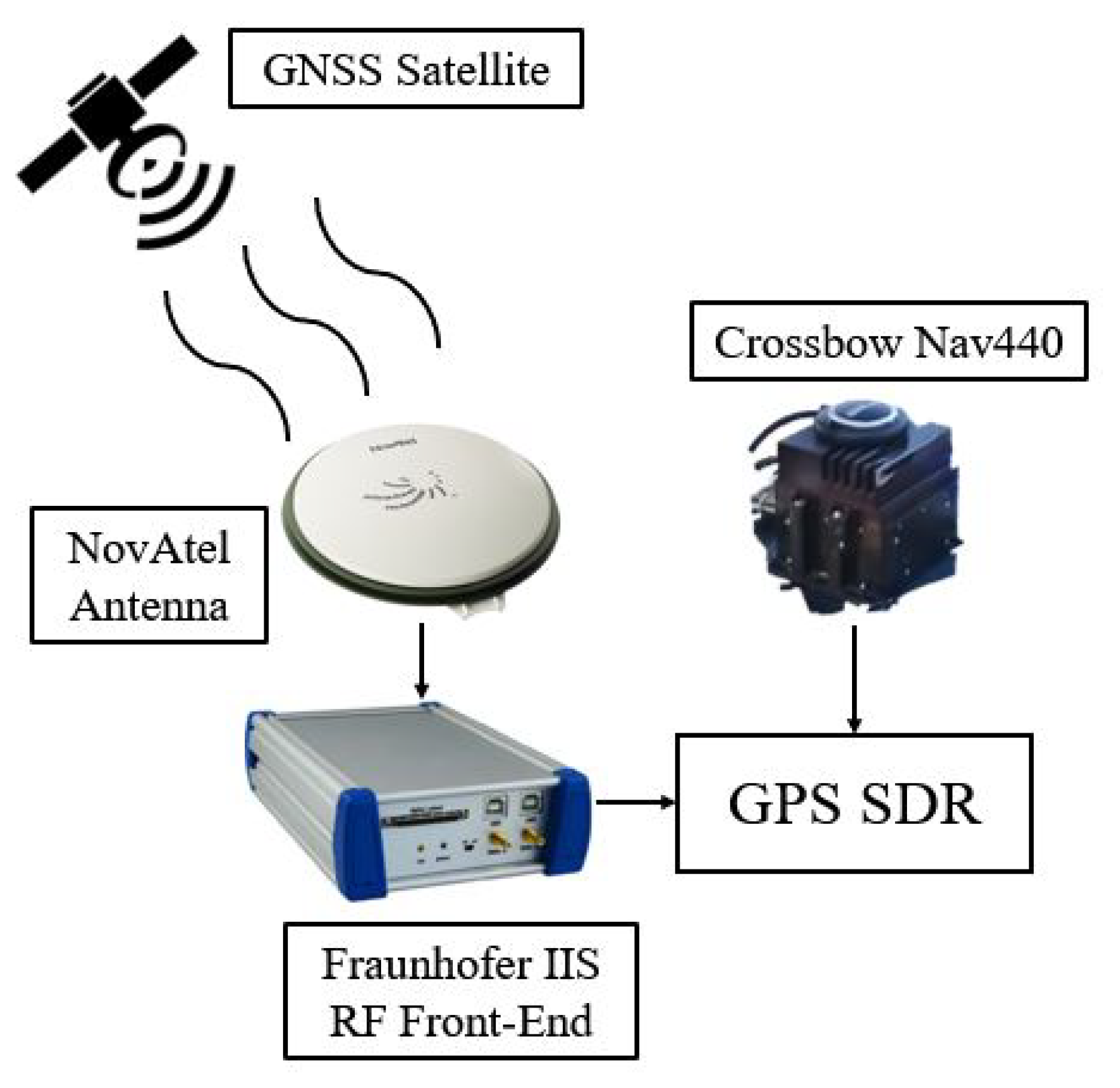
The experimental equipment was set up as shown in
Figure 5. Two stationary data sets were collected in the real world to verify the proposed algorithm. A NovAtel antenna was used to receive the GPS L1 C/A IF signals through a Fraunhofer IIS RF frond-end, where the IF sampling rate was 10.125 MHz. The IMU raw data were collected from the Crossbow Nav 440 device, where the IMU’s gyro and accelerometer bias stability were 10 deg/h and 1 mg, respectively. It is worth mentioning that two samples were taken for updating the inertial sensor data for our navigation equation, so the updating rate of the INS DR was half (50 Hz) of the IMU raw data rate (100 Hz).
The reference positions of the two experiments were obtained by averaging the results provided by the Crossbow Nav440 GPS/INS integration solutions (the centers of the IMU sensor and the GNSS antenna were sufficiently close in the setup and neglected in this experiment). The reference position was accepted to validate the experiment. First, the experiment tested the GPS L1 C/A code signal, of which the code chip was around 293 m. Second, by observing the reference position, compared to the parking lines in Google Maps in the following positioning results, it was possible to approximately infer that the biased position error of the reference did not exceed 20 cm, as most of the random errors and only minor biased errors remained after the averaging operation. Third, the following ground-truth-based hardware-in-the-loop (HIL) test outperformed the positioning accuracy of all the other algorithms. So, the reference coordinates were acceptable in this experiment.
The proposed algorithm was tested in a GPS SDR platform where the coherent integration time was 5 ms, the classic discriminators were chosen as the noncoherent-early-minus-late-amplitude code discriminator and Costas carrier discriminator, and the early-late spacing was four IF sample intervals. Five types of tracking algorithms were compared in the same SDR conditions except for the parameter adjustment in
Table 1.
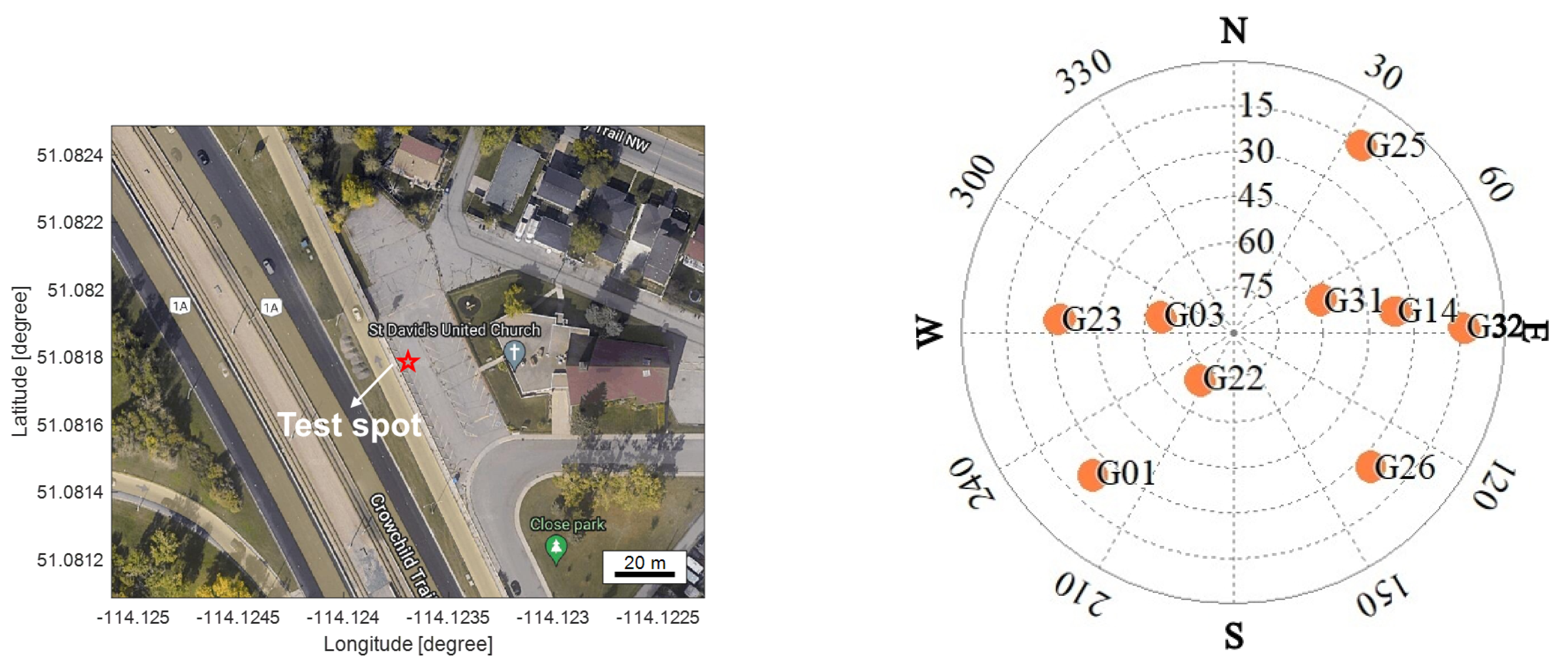
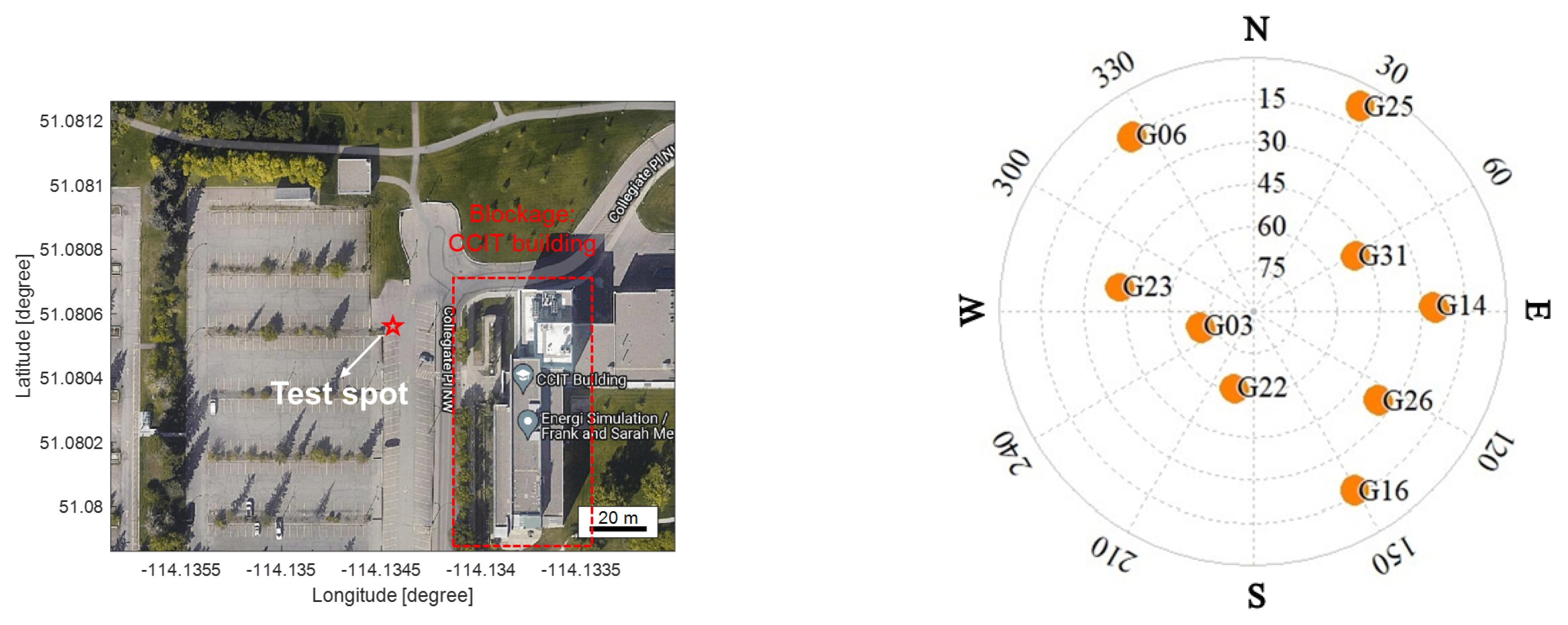
First, an open sky area was chosen to carry out the experiment. The test spot in Google Map and the sky plot of the available GPS satellites are shown in
Figure 6.
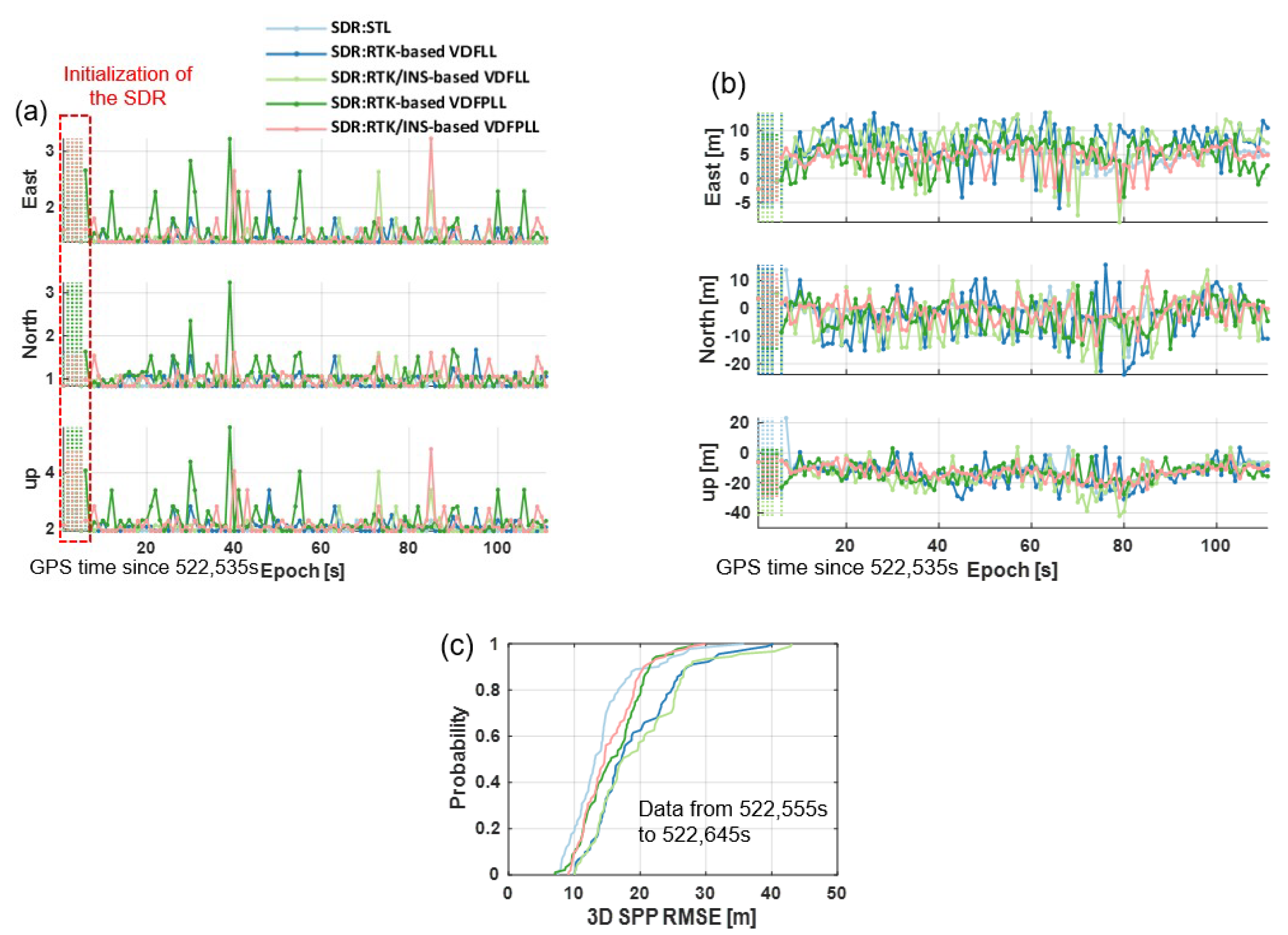
We first assessed the SPP results for the open-sky case. The SPP was based on the weighted NLS algorithm in the tested SDR, which referred to an open-source package RTKLIB [
39].
Figure 7 depicts the dilution of precision (DOP) results, SPP errors, and the 3D position cumulative distribution function (CDF) curves of 3D SPP root-mean-squared errors (RMSEs).
Although the results showed that the proposed algorithm did not increase the SPP accuracy compared to the classic STL algorithm in the open sky, they proved that the APA-based VDFPLL algorithms enhanced the traditional RPA-based VDFLL in the static situation. Meanwhile, using the INS could moderately enhance the RTK-based APA tracking process.
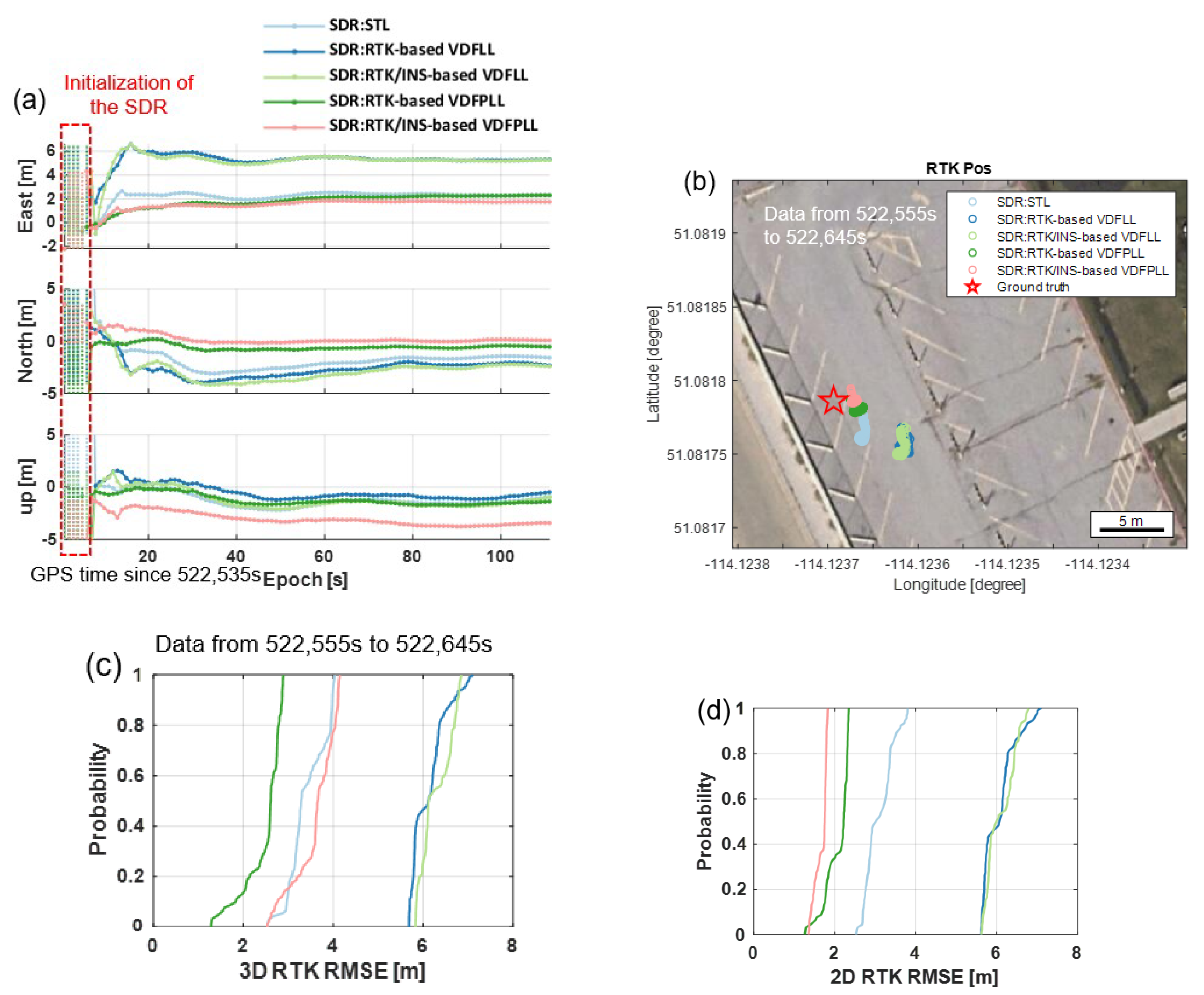
Then, the RTK position errors for the different SDR algorithms were compared in
Figure 8, where the position errors, horizontal position results for a Google Map show, and the CDF curves of 3D and 2D position estimates RMSE were included. The traditional RPA VDFLL did not help the RTK position accuracy in the open-sky and static case. The finding was that the RTK-based VDFPLL (i.e., the VDFPLL relied on the position solution solely computed from the RTK algorithm) improved the RTK results within a 3D range, while the RTK/INS-based VDFPLL slightly outperformed the STL-based horizontal positioning. The vertical INS DR position solution would cause more code phase errors (compared to the STL tracking in a static open-sky case) in terms of the vertical position estimation.
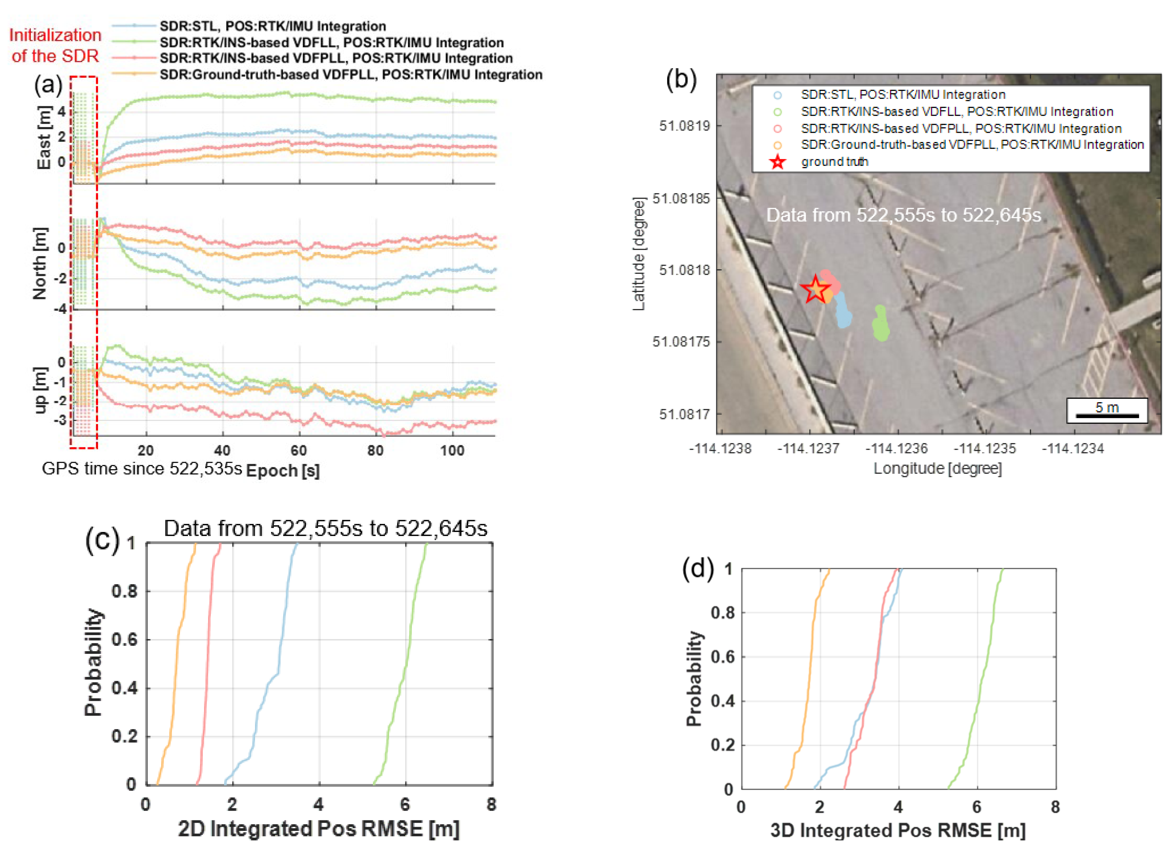
Next, we compared the RTK/INS integrated results of three SDRs in
Figure 9, where “Ground-truth-based VDFPLL” meant that the SDR leveraged the actual position coordinates instead of on-the-fly RTK or integrated RTK/INS position estimates. It was a HIL simulation strategy to provide a reference for the proposed algorithm under the same SDR conditions. In other words, the HIL simulation results represented the upper bound of the performance that the SDR platform used could achieve.
Based on the CDF curves in
Figure 9d, the proposed accuracy slightly exceeded the traditional STL-based integrated RTK/INS solution within the 78% probability. So, the large errors could be alleviated in the integration results using the proposed algorithm in the open sky area. In contrast, the traditional VDFLL-based integrated RTK/INS positioning accuracy decreased a lot in this well-conditioned static scenario.
TOA curves are evaluated on to examine the baseband processing discrepancy. The TOA estimation from the GPS SDR was computed via (
3), where the
was the raw data from the loop filter output without the carrier-smoothing algorithm. Therefore, the measurement and reference TOA residuals in meters were computed as follows
where the TOA residuals excluded the initial pseudorange and initial Doppler frequency for the simplicity of analysis; subscript 0 and
k denote the initial and the
kth epoch, respectively;
and
represent the TOA and Doppler frequency reference at the initial epoch, and they are computed as
where
and
are the ground truth vectors in the ECEF coordinate frame for the user’s position and velocity in the stationary experiments, with
;
,
,
, and
are the satellite position and velocity vectors, satellite clock bias and drift errors, respectively, which were obtained and computed using the broadcast ephemeris. Meanwhile,
and
were the ionospheric error derived from the Klobuchar model and the tropospheric error calculated via the Saastamoninen model.
is the unit cosine vector computed from
;
and
are the estimated user’s clock bias and drift errors computed as
where
is the averaging value of the clock drift estimates from the “Ground-truth-based VDFPLL” SDR.
The given and references were not sufficiently accurate, but they were satisfactory in validating the TOA performance amidst the different SDR algorithms.
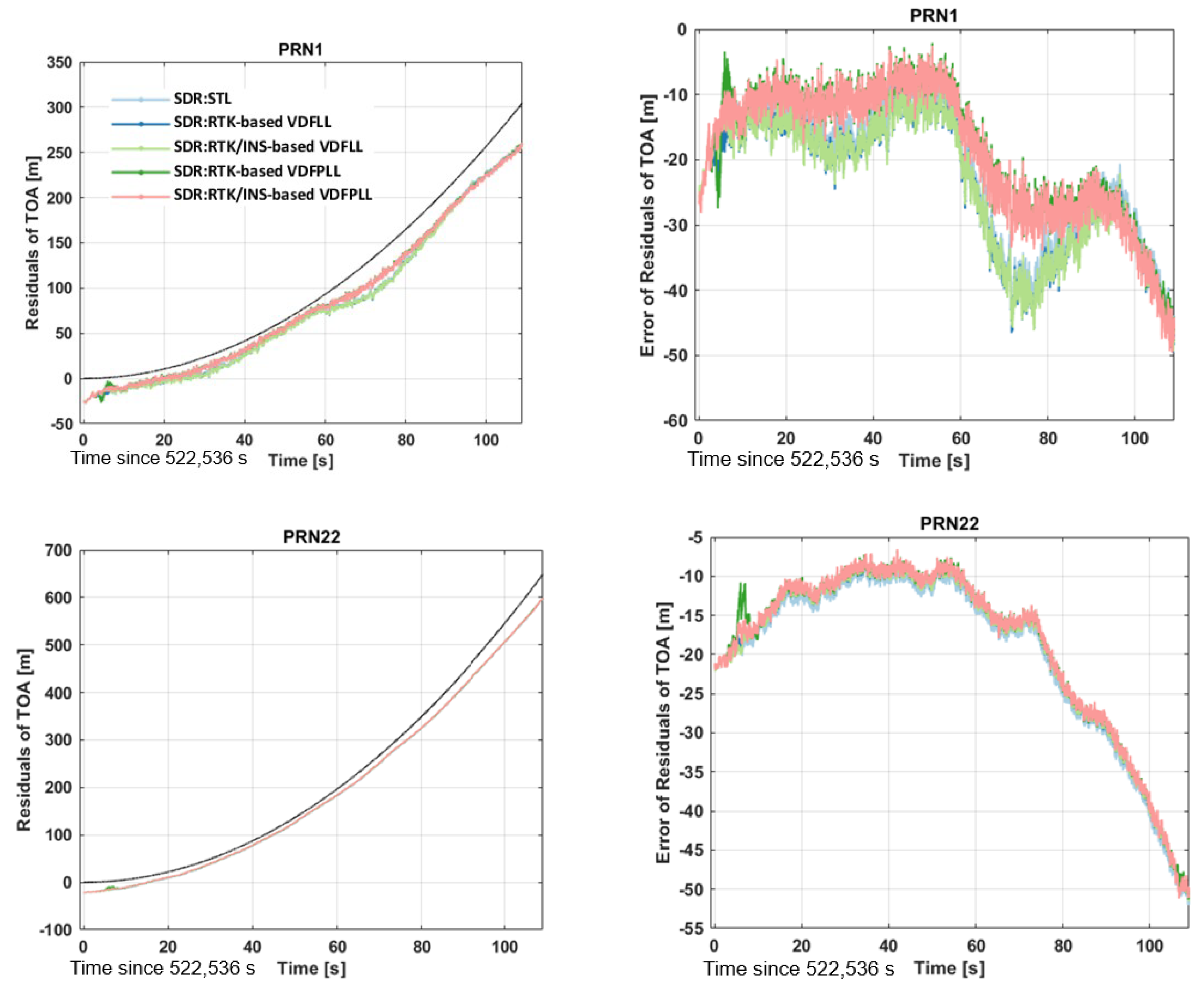
Figure 10 shows the error curves of the TOA residuals for the signals from the satellite of PRN1 (low elevation angle) and PRN22 (high elevation angle). It was proved that the APA-based vector tracking algorithms performed better in interference mitigation for the signals from the low satellite.
In summary, even if the proposed algorithm did not manifest results much better than the traditional STL in an open-sky static environment, it demonstrated a significant improvement in comparison with the traditional RPA vector tracking in the same condition. More specifically, it could be used as a boosting complement for the existing vector GNSS receivers.
Another set of data was collected under a semi-open-sky situation where the GPS antenna was receiving the signals affected by the eastern CCIT building at the campus of the University of Calgary. The Google Map of the test spot and the corresponding satellite sky plot are provided in
Figure 11.
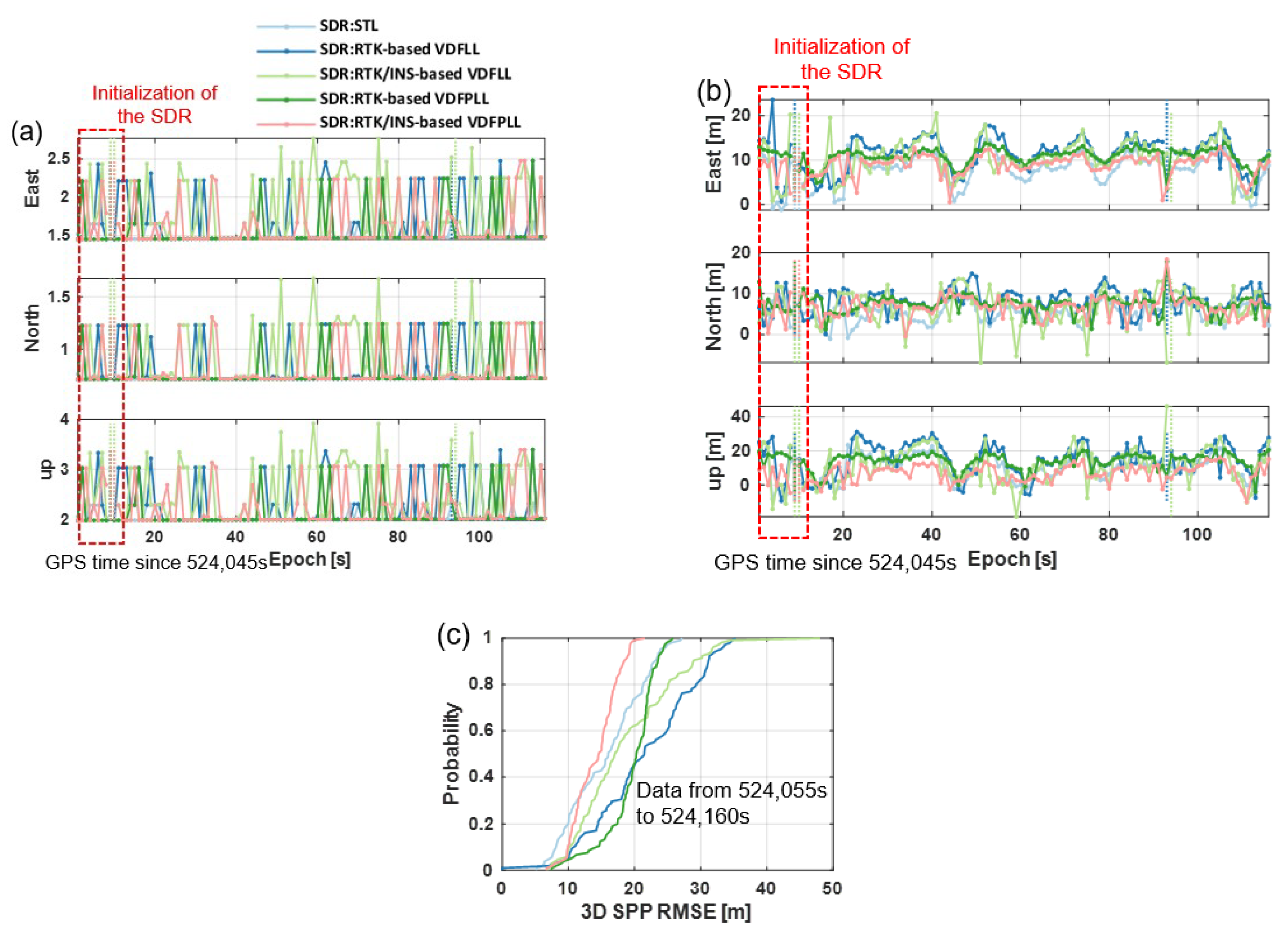
In this test, where the results are displayed in
Figure 12, we also provided the DOP values to offer the satellite geometry status. The SPP error curves and their 3D CDF were provided as well.
First, it can be observed that the two VDFPLLs and the STL produced more reliable solutions than the position outliers of the two VDFLLs at around the 95th epoch. It is evident that the proposed algorithm embraced the highest SPP accuracy.
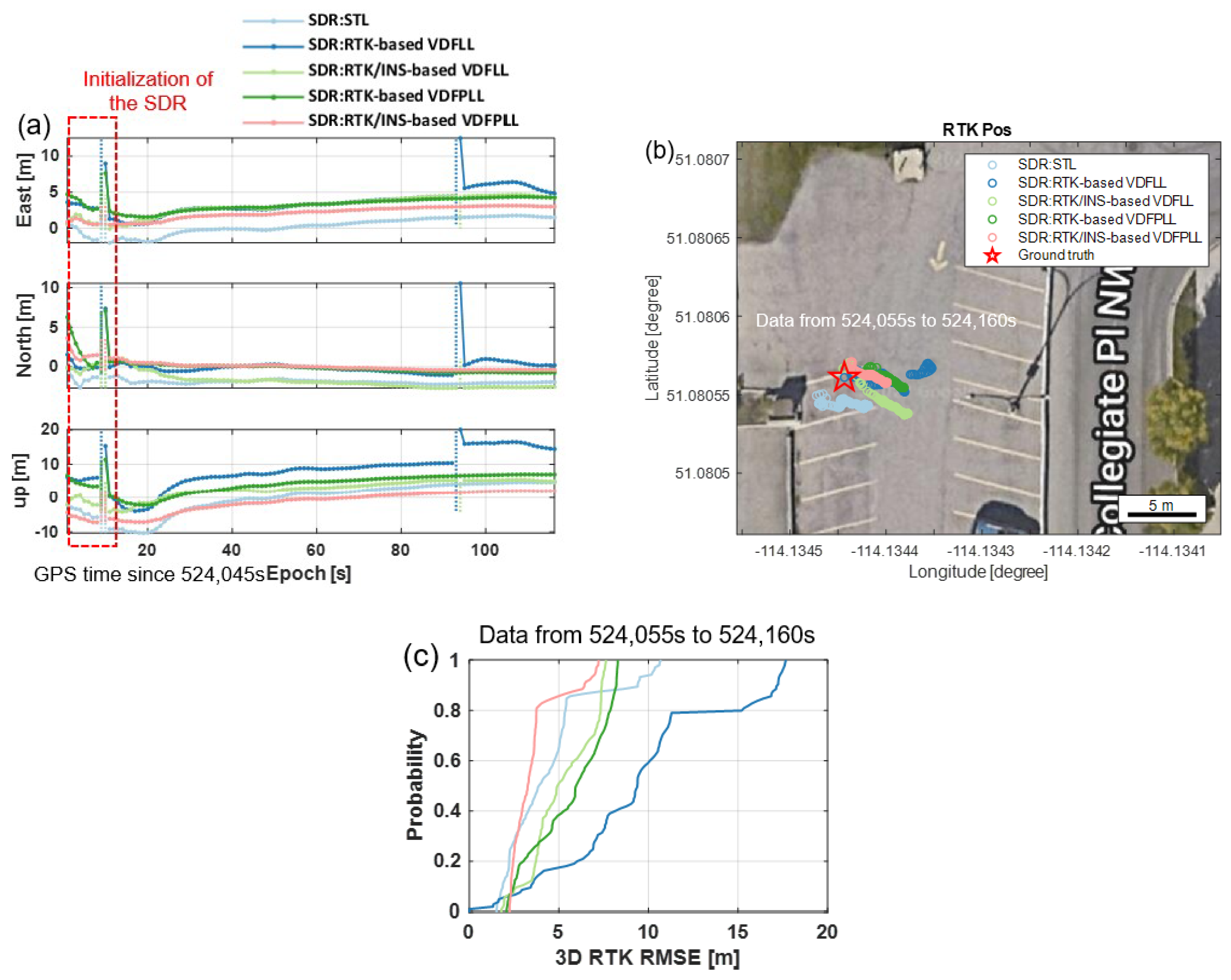
We also assessed the RTK solution accuracy related to the different SDRs. The RTK position error curves, position results in Google Map, and the 3D CDF curves are provided in
Figure 13. After the SDR RTK solutions became stable, the RTK accuracy from the proposed SDR solutions still showed the highest performance. The RTK-only-based APA algorithm could reduce the random noise, but it was more biased than the traditional STL algorithm. The two RPA-only vector tracking techniques were still less capable of offering efficient assistance in the static test.
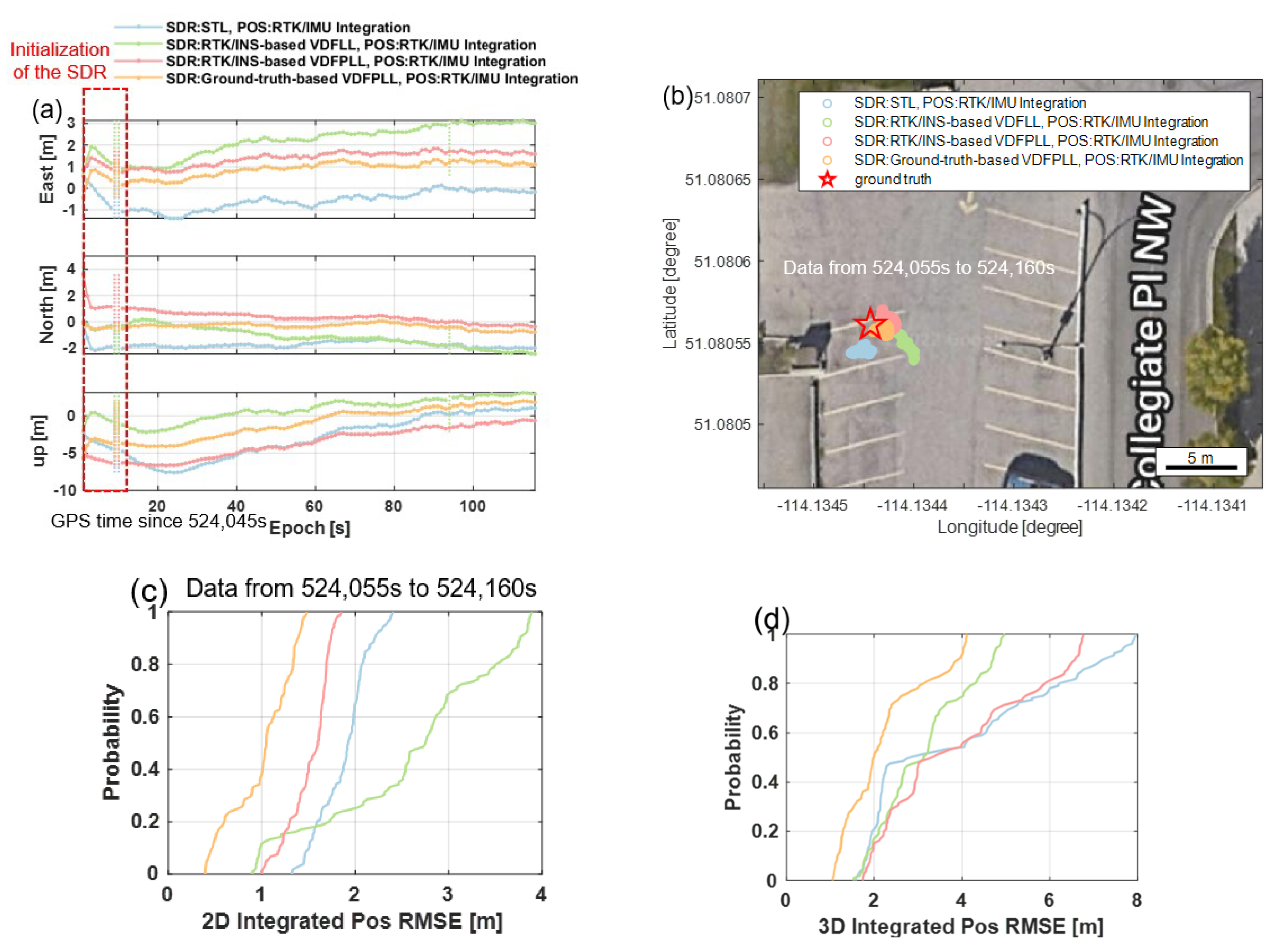
Next, the integrated RTK/INS solutions were compared in the semi-open-sky environment, as shown in
Figure 14. In this case, the proposed algorithm significantly improved the 2D positioning performance. At the same time, the RTK/INS-based RPA method elevated the 3D positioning accuracy, compared to the STL-based integration. The RPA- and APA-based integrated navigation accuracies over the error range of approximately 55% probability outperformed the traditional STL one. Furthermore, the positioning results with the proposed algorithm performed more stably than the traditional vector tracking. Another finding was that RTK/INS-based APA vector tracking yielded a much more ideal horizontal positioning estimate than the RPA one. By contrast, the latter was superior to the former in the vertical direction. By comparing to the upper bound (i.e., the estimation from the ground-truth-based VDFPLL SDR), the fusion of the low-cost IMU had a side effect on the vertical position solution when it was applied to the proposed RTK/INS-based VDFPLL SDR in this stationary experiment.
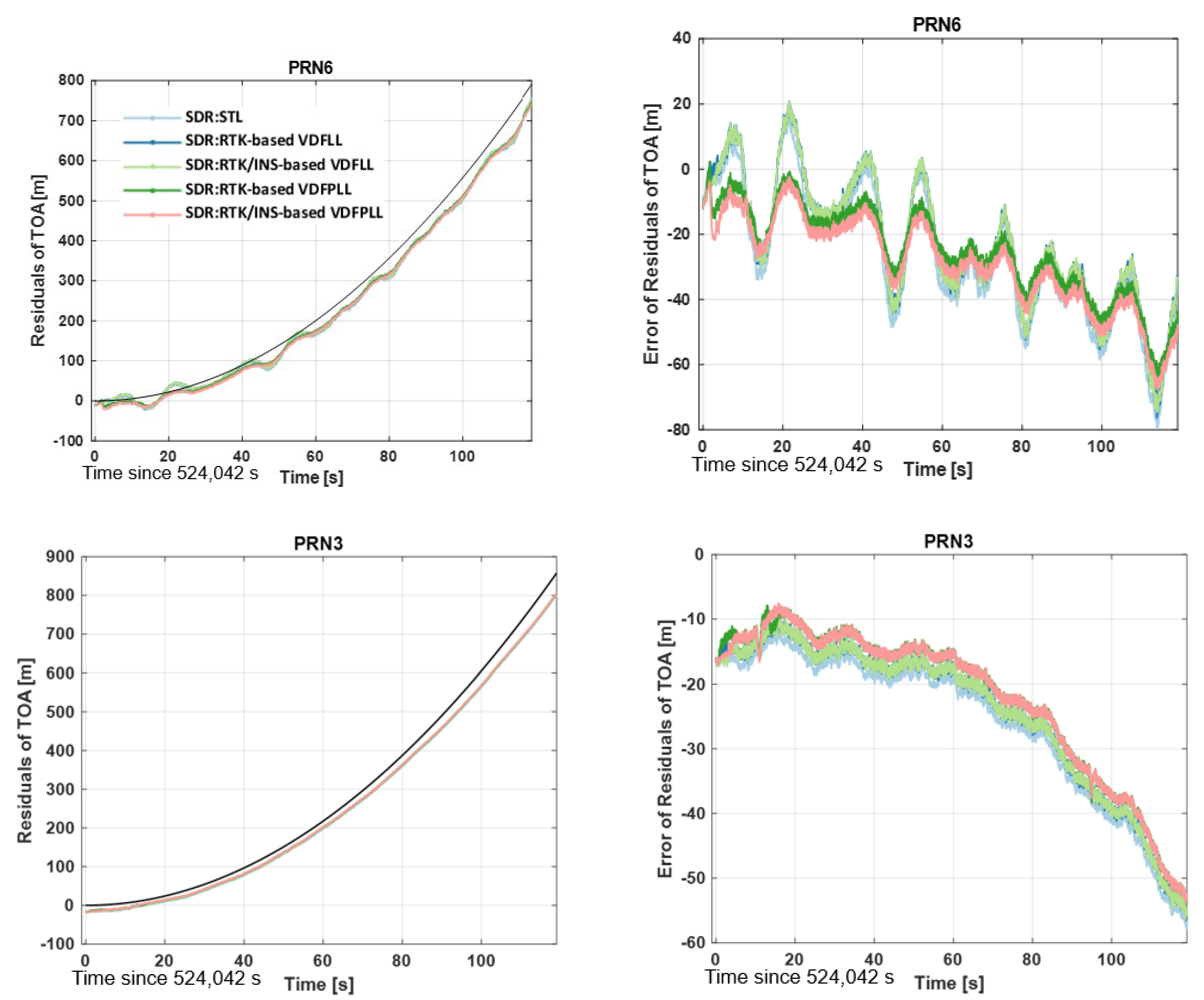
Then, the raw TOA performance, in terms of the signal from the high-elevation-angle satellite (PRN3) and the one with a low elevation angle affected by the multipath interference (PRN6), were plotted in
Figure 15. A more significant fluctuation in the TOA curves emerged at the PRN6 in this semi-open-sky experiment, compared to the open-sky PRN1 (see
Figure 10). Both APA-based tracking loops were more capable of alleviating the TOA error varying with long-term time spanning (i.e., the level of dozens of seconds) than the RPA-based vector tracking and the STL. Nevertheless, the curves computed from the high-quality signal, PRN3, were highly homogeneous regarding all the tested tracking loop algorithms.
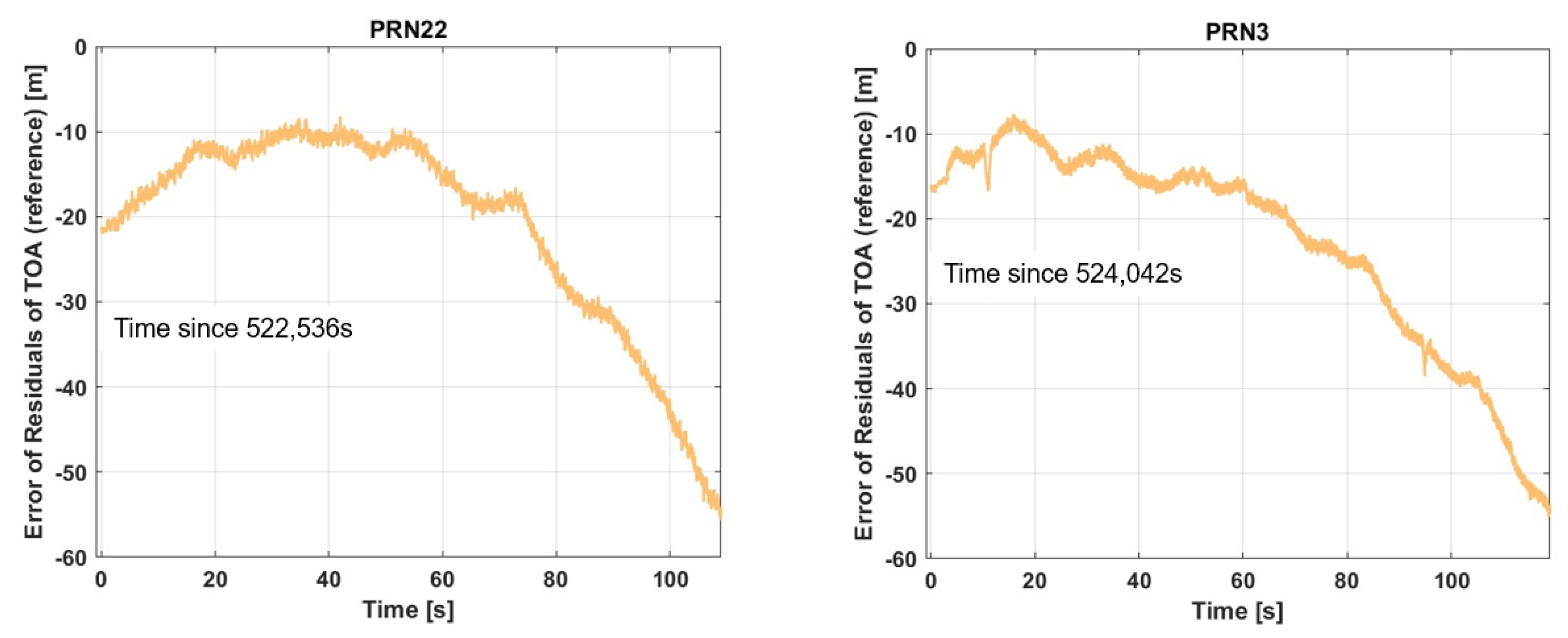
The next part quantitatively examines the exact improvement the proposed algorithm could offer for the GNSS baseband estimation. As mentioned, an upper bound of the instantaneous integrated positioning performance was obtained from the SDR under the HIL test using the “Ground-truth-based VDFPLL”. Therefore, the corresponding TOA error curve, representing the upper bound, could also be extracted from the tracking results. Then, we computed the TOA error of the PRN22 and PRN3 (with the highest elevation angles during the experiments) in the open-sky and semi-open-sky cases as the respective references. The proposed TOA error references reasonably modeled the remained local clock errors in meters, varying with time. The other biased errors, like the atmospheric delay and initial TOA errors, were assumed to be well removed by the given models.
Ultimately, the TOA curve references were derived and are illustrated in
Figure 16. After that, the TOA accuracy of different satellites in the two testing situations was analyzed via these references in the following.
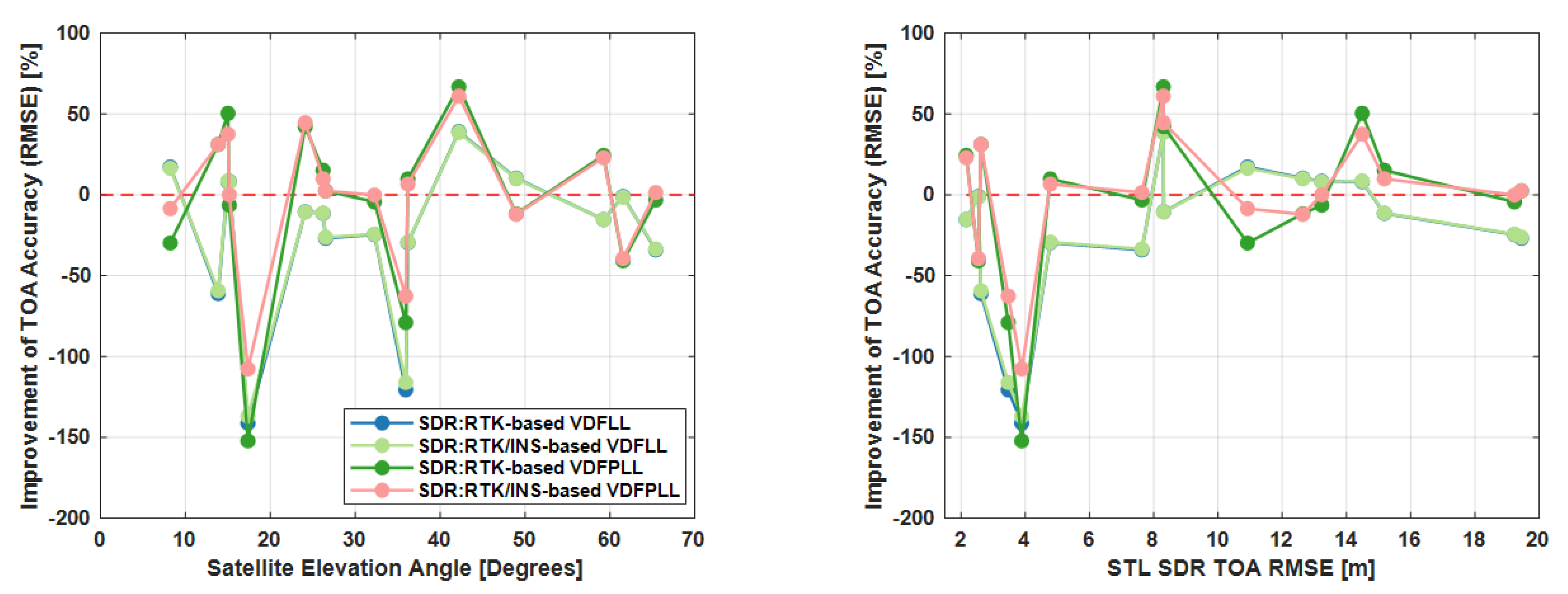
Table 2 summarizes the statistical analysis of the TOA performances of different tracking algorithms where the RMSE results were computed for the satellites used. Then, in regard to the traditional STL, the TOA accuracy improvements of the two RPA- and APA-based vector tracking algorithms operating in the GPS SDR were computed and are depicted in
Figure 17.
The curves in
Figure 17 indicate that both APA tracking methods outperformed the two RPA ones in elevating TOA accuracy. Furthermore, regarding the lower-elevation satellites and the smaller-TOA-error channels, the TOA errors induced by the navigation results through the vector feedback procedure were more likely to drop in the proposed RTK/INS-based APA approach than in the RTK-only APA one.
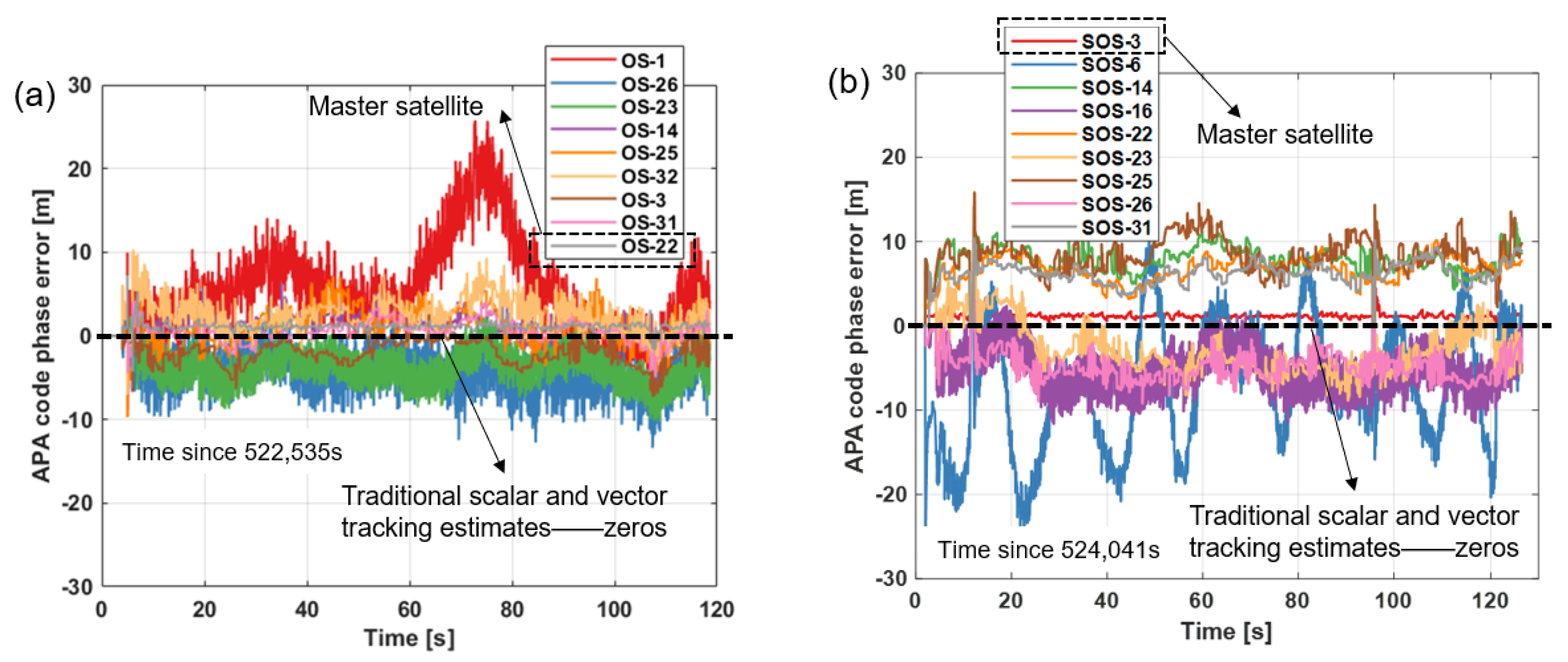
Figure 18 plots the APA error curves estimated from the proposed RTK/INS-based VDFPLL modeling the instantaneous initial/absolute code phase error in meters at each tracking epoch. The analytical expression is given by (
15). Compared to the traditional tracking algorithms (scalar and old vector tracking loops), the proposed algorithm could individually discriminate the absolute code phase error unrelated to the frequency error given by the same epoch local replica subtracting incoming signals. This operation established through the proposed architecture was reasonable and it proved efficient. The implication from the results was that the RTK/INS integrated EKF navigator provided more accurate positioning than the code-based-only SPP method.
So, the dashed black lines in
Figure 18 mean that the traditional scalar and vector tracking loops had nothing to recognize the code phase error not varying with the time spanning (the error residual remaining from the traditional code discriminating process). However, the proposed RTK/INS-based APA vector tracking could directly estimate the absolute code phase error at every tracking epoch. The APA code discriminated results showed how the code phases were corrected by the accurate user’s position solution, especially for the satellites wherein the deterministic biased error changed in cycles of dozens of seconds or longer. This phenomenon commonly occurs to static user antenna receiving incoming signals affected by the multipath effect.
Finally, it is worth mentioning that the proposed RTK/INS-based VDFPLL was a simplified prototype applying the APA discriminated error relying on the INS and RTK to the GNSS baseband processing. The tracking performance still has space to be further improved by redoing loop filter algorithms (e.g., the EKF) or other GNSS baseband optimizing methods (e.g., snapshot processing [
40,
41] and open-loop tracking [
42,
43]). In other words, the proposed algorithm has a broad scope of use towards GNSS signals at all frequencies and constellations, potentially contributing to the development of next-generation GNSS receivers and GNSS-based multi-sensor integrating navigation systems.

 ,
, 


