

A Novel Real-Time Edge-Guided LiDAR Semantic Segmentation Network for Unstructured Environments
School of Instrument Science and Engineering, Southeast University, Nanjing 210096, China
*
Author to whom correspondence should be addressed.
Remote Sens. 2023, 15(4), 1093; https://doi.org/10.3390/rs15041093
Submission received: 12 January 2023
/
Revised: 10 February 2023
/
Accepted: 13 February 2023
/
Published: 16 February 2023
(This article belongs to the Special Issue Development and Application for Laser Spectroscopies)
Abstract
:LiDAR-based semantic segmentation, particularly for unstructured environments, plays a crucial role in environment perception and driving decisions for unmanned ground vehicles. Unfortunately, chaotic unstructured environments, especially the high-proportion drivable areas and large-area static obstacles therein, inevitably suffer from the problem of blurred class edges. Existing published works are prone to inaccurate edge segmentation and have difficulties dealing with the above challenge. To this end, this paper proposes a real-time edge-guided LiDAR semantic segmentation network for unstructured environments. First, the main branch is a lightweight architecture that extracts multi-level point cloud semantic features; Second, the edge segmentation module is designed to extract high-resolution edge features using cascaded edge attention blocks, and the accuracy of extracted edge features and the consistency between predicted edge and semantic segmentation results are ensured by additional supervision; Third, the edge guided fusion module fuses edge features and main branch features in a multi-scale manner and recalibrates the channel feature using channel attention, realizing the edge guidance to semantic segmentation and further improving the segmentation accuracy and adaptability of the model. Experimental results on the SemanticKITTI dataset, the Rellis-3D dataset, and on our test dataset demonstrate the effectiveness and real-time performance of the proposed network in different unstructured environments. Especially, the network has state-of-the-art performance in segmentation of drivable areas and large-area static obstacles in unstructured environments.

1. Introduction
Scene understanding is crucial to ensure the reliability of autonomous vehicles and mobile robots in outdoor environments. As the core of scene understanding, semantic segmentation that provides fine-grained object labels is a challenging problem in computer vision. Since semantic segmentation can obtain various information such as the category and shape of objects, it is widely used in mobile robots [1,2], autonomous driving [3,4], medical diagnosis [5,6], and other fields.
Currently, significant progress has been made in the field of autonomous driving with existing semantic segmentation methods [3,7,8]. These methods mainly focus on structured environments, such as the common urban road environment. Due to the limited variation of scenes and the presence of distinct structured edges between classes, structured environments are relatively easy to segment accurately. Unstructured environments mainly include less structured rural environments, off-road environments, and rescue environments, etc. Most of these scenes are characterized by blurred class edges, irregular class geometric features, and irregular lighting changes. These characteristics are more apparent in unstructured drivable areas and static obstacles with large areas, which often account for more than 75% or even up to 90% of the unstructured environment, making the existing semantic segmentation methods perform poorly. Therefore, the study of semantic segmentation for unstructured environments is important for scene understanding and subsequent autonomous driving decisions.
Typically, semantic segmentation is performed using images or LiDAR (light detection and ranging) point clouds. There are already several camera-based methods for segmenting unstructured environments [9,10]. However, the similarity in colors of the background, obstacles, and roads in unstructured environments and the instability of the camera under changing illumination make camera-based methods vulnerable to color and texture features that are not robust enough [11]. In contrast, LiDAR can acquire geometric features of the surrounding environment to better distinguish between obstacles and roads, and thanks to the active illumination sensor, it is not affected by changes in ambient light and has a strong anti-interference ability. Recently, LiDAR-based semantic segmentation of unstructured environments has been developed. On the one hand, most methods use voxel-based [12] or point-based [13] methods for feature extraction, which not only do not design targeted network structures for the edge blurring problems, resulting in poor results when segmenting drivable areas and static obstacles with large areas but also do not guarantee real-time segmentation. On the other hand, some methods are trained only for certain unstructured environments, such as bush segmentation in agricultural scenes [14], and are therefore less adaptable.
To address the above issues, we propose a novel real-time edge-guided semantic segmentation network to simultaneously improve the accuracy and adaptation of semantic segmentation in unstructured environments, especially for drivable areas and static obstacles with large areas in it. Thanks to the full exploitation of the edge information of the point clouds, the discrimination ability of pixels near the edges between classes and the extraction ability of features in an unstructured environment improve greatly, which in turn promotes a more accurate and robust performance of the proposed method. The main contributions of this article are as follows:
- We propose a novel edge-guided network for real-time LiDAR semantic segmentation in unstructured environments. The network fully exploits edge cues and deeply integrates them with semantic features to solve the problem of inaccurate segmentation results in unstructured environments due to blurred class edges. Compared with state-of-the-art point clouds segmentation networks, the proposed network performs better in the segmentation of unstructured environments, especially in drivable areas and static obstacles with large areas;
- We design an edge segmentation module which contains three edge attention blocks. Different from the published point clouds semantic segmentation methods, this module adaptively extracts high-resolution edge semantic features accurately from the feature maps of the main branch in a supervised manner, which improves the accuracy of edge segmentation on the one hand, and provides edge guidance for semantic segmentation of the main branch on the other hand, thus helping to capture edge features of classes in unstructured environments more effectively;
- We design an edge guided fusion module to better fuse edge features and semantic features, and improve the discrimination of pixels around edges between classes. Different from the traditional feature fusion methods, this module fully exploits the multi-scale information and recalibrates the importance of different scale features through a channel-dependent method, effectively utilizing the complementary information of edge features and semantic features to further improve the segmentation accuracy of the model.
2. Related Work
This section mainly reviews the related semantic segmentation methods in three aspects, including semantic segmentation of large-scale point clouds, semantic segmentation of unstructured environments, and edge improved semantic segmentation.
2.1. Semantic Segmentation of Large-Scale Point Clouds
Semantic segmentation, the task of labeling each pixel of an image with the corresponding category of what is being represented, is the key to scene understanding for unmanned platforms. Thanks to the richness of public datasets, camera-based semantic segmentation algorithms of urban environments have made great progress; however, cameras are heavily influenced by the level of illumination, which limits the operating environment of unmanned platforms. As a result, LiDAR-based semantic segmentation algorithms for urban environments have also received a wide range of attention from researchers in recent years. Currently, there are several well-performing methods for the semantic segmentation task of point clouds in urban environments: point-based methods, voxel-based methods, and range-based methods.
Point-based methods extract features based primarily on the structure and spatial topological relationships of the point clouds itself. Some methods such as PointNet [15], Pointnet++ [16], and KPConv [17], directly use raw point clouds for feature extraction, but these methods are less effective in dealing with large-scale point clouds due to high computational costs and limited receptive fields. To expand the receptive field and improve the inference speed, RandLA-Net [18] proposes a network structure with efficient random sampling and local feature aggregation, but random sampling may result in the loss of features in certain regions, which may lead to the deletion of key points in unstructured road environments and affect the segmentation results.
Voxel-based methods [19,20,21,22] retain more complete 3D geometric information by converting point clouds into 3D voxels. However, due to the sparsity of the point clouds data, the accuracy of the algorithm depends on the density of the 3D mesh [23], so, it is difficult to balance between real-time and accuracy given the large number of operations involved in 3D convolution.
Range-based methods [24,25,26,27,28] map 3D point clouds to 2D images by spherical projection and extract features from projected images using 2D convolution. This approach can effectively decrease the amount of data and realize semantic segmentation in real time. SqueezeSeg [24] and SqueezeSegv2 [25] convert point clouds to 2D images and do feature extraction and optimization of segmentation results based on SqueezeNet and conditional random field (CRF) for point clouds. RangeNet++ [26] reduced discretization errors in the process of back-projection by using accelerated KNN for post-processing; KPRNet [27] employs a strong backbone and uses KPConv [17] as a segmentation head, achieving better results. However, since spherical projection maps 3D point clouds to 2D images, it inevitably results in distortion of physical dimensions and loss of some geometrically related spatial information.
The above methods achieve good results in point cloud semantic segmentation in urban environments, but they are not customized for the unstructured environments.
2.2. Semantic Segmentation of Unstructured Environments
Some works use traditional rule-based or threshold-based methods to extract traversable regions [29,30]. However, these methods rely on artificially designed features or pre-set thresholds which are poorly adaptable to varied scenarios. Besides, they only focus on drivable area extraction and do not provide a comprehensive perception of the environment. Therefore, the segmentation of unstructured environments using deep learning methods is gradually gaining attention from researchers.
Zhu et al. [12] proposed a network to enhance the road boundary which uses the RANSAC algorithm to extract the road boundaries of point clouds and fuse them with the features of the original point clouds to segment the road more effectively. There are also some methods that only train for specific unstructured environments. For example, Chen et al. [13] propose an improved RandLA-Net to be used in large-scale unstructured agricultural environments. Wei et al. [14] propose a new BushNet for effective segmentation of bush point clouds in the agroforestry scenes. The above methods mainly use point-based or voxel-based methods in point clouds for semantic segmentation. However, these two methods are insensitive to edges. In point-based methods, the downsampling algorithm causes the point clouds to lose critical edge information, while in voxel-based methods, different classes of points on either side of the edge may be mixed in a single voxel near the edge. Both methods also make it difficult to ensure a balance between accuracy and real-time performance. At the same time, scene-specific feature extraction leads to poor adaptability of the methods.
2.3. Edge Improved Semantic Segmentation
In the field of 2D image-based scene understanding, edges, as an important part of images, are useful for improving semantic segmentation performance. Early studies [31,32] mainly focused on introducing edge information in the post-processing step. However, they do not fundamentally improve the accuracy of semantic segmentation. Peng et al. [33] introduced a residual-based edge refinement method to improve the performance of localization around the object edges, which uses edges as an intermediate feature to improve segmentation accuracy. Moreover, some methods extract edge features separately through the edge detection branch, and these features are used to guide the task of the main branch. Yu et al. [34] proposed a discriminative feature network (DFN) containing a border network to improve the inter-class distinction. Takikawa et al. [35] designed an edge detection stream, called shape stream, which enables the segmentation model to better capture the edge information of the object, thus enabling more accurate segmentation of small objects. Ma et al. [36] proposed a boundary-guided context aggregation method to facilitate the overall semantic understanding of images. The method enables internal pixels of the same class to achieve mutual gain, which improves intra-class consistency.
In the field of 3D-point-clouds-based scene understanding, current edge improved methods are mainly for indoor areas, for example, Gong et al. [37] proposed a boundary prediction module and used the prediction results to aid in improving the segmentation performance. Hu et al. [38] proposed JSENet to solve the semantic segmentation and class-aware semantic edge detection problems in a joint learning manner. Hao et al. [39] proposed a mixed feature prediction strategy to pretrain a boundary-aware model. These representative methods are designed for indoor scene semantic segmentation datasets with more detailed semantic label definitions and more densely connected objects, such as S3DIS [40] and ScanNet [41] datasets. In these datasets, the point clouds are small-scale, dense, and evenly distributed. In contrast, in the outdoor scene dataset, the point clouds are large-scale, sparse, and unevenly distributed. Meanwhile, these point-based methods are computationally inefficient in large outdoor environments and is not suitable for scenarios with high real-time requirements such as autonomous driving.
Our work uses an efficient spherical projection method to LiDAR point clouds data and proposes an edge-guided semantic segmentation network for unstructured environments inspired by the edge improved methods for 2D images, which alleviates the problems of unclear class edges in the unstructured environment, and is more adaptable to various unstructured environments.
3. Methods
3.1. Network Overview
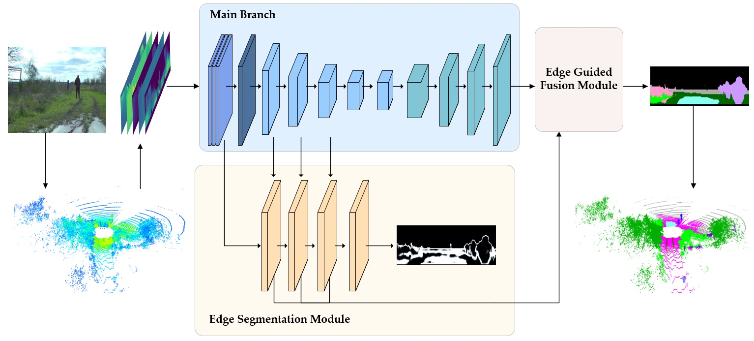
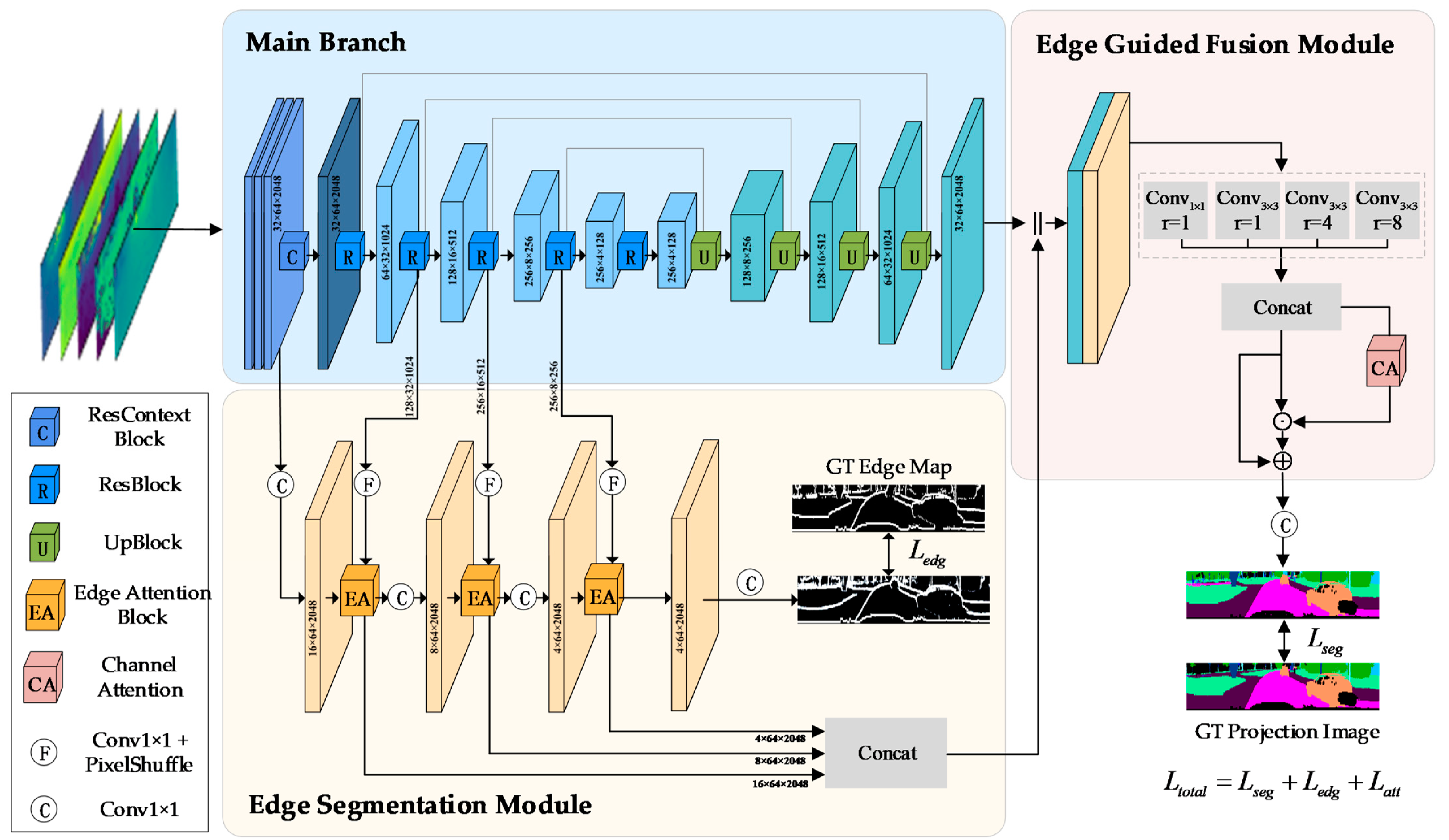
We propose a novel edge-guided network to perform real-time point clouds semantic segmentation, as shown in Figure 1. The proposed network constitutes three parts: main branch, edge segmentation module, and edge guided fusion module. The main branch acquires shallow and deep semantic feature maps for subsequent feature fusion. As a contrast, the edge segmentation module adaptively filters out edge-independent information from the feature maps at different resolutions in the main branch using a set of residual blocks and edge attention blocks (EAB). Moreover, the accuracy of the extraction of contextual information from the pixels around the edge is ensured by the additional supervision of the edge map. The output of the main branch and the cascaded EABs are simultaneously fed into the edge guided fusion module through four parallel convolutional layers, and the multi-scale contexts are captured. Then, the fused features are fed into the channel attention module to suppress redundant information and recalibrate channel-wise feature responses thus obtaining better segmentation results.
3.2. Data Pre-Processing
3.2.1. Pre-Processing of Input Data
As in RangeNet++ [26], we used the spherical projection method to generate 2D range images as the input to the network. In the range images, each LiDAR point is converted to image coordinates .
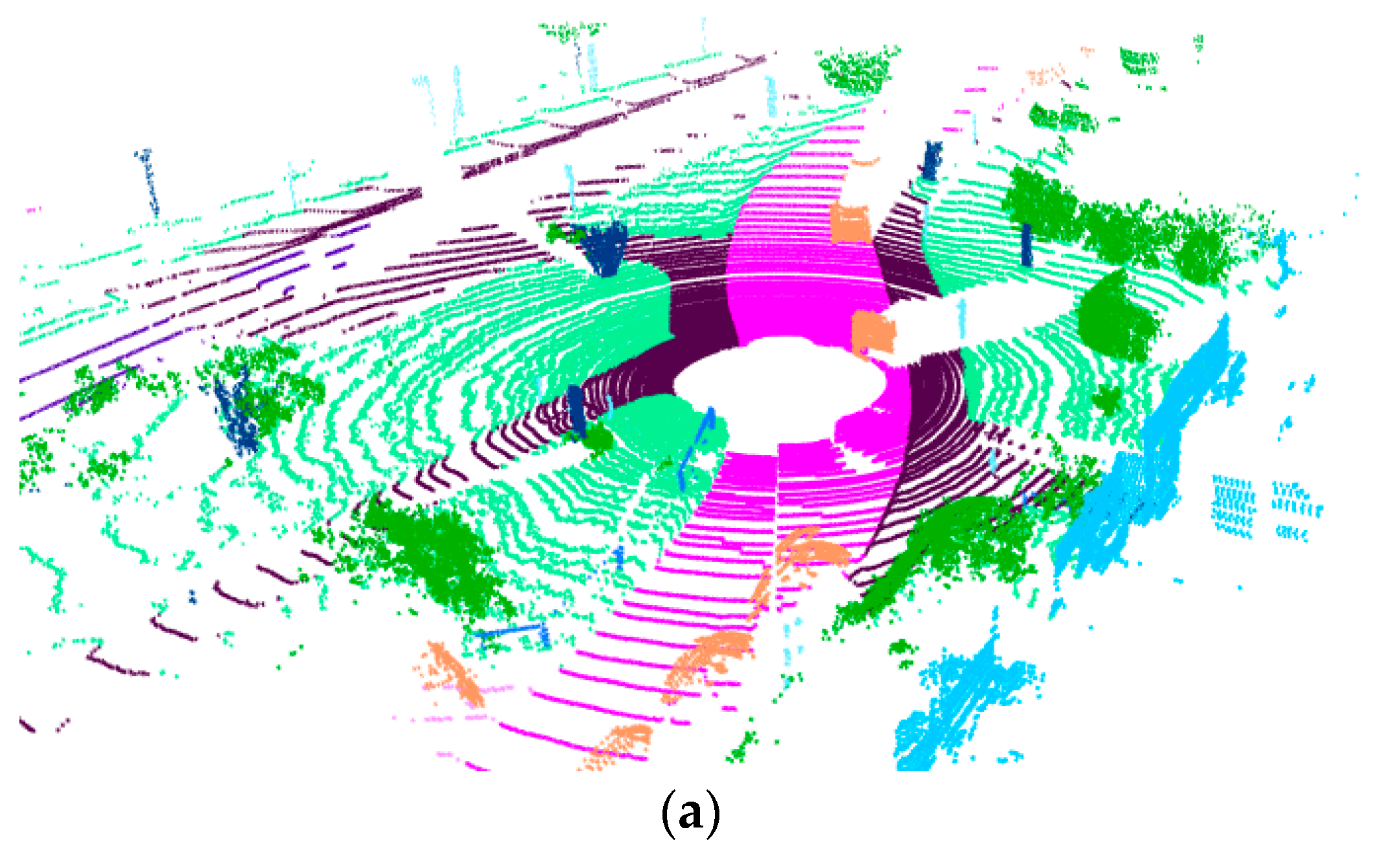
After the projection, we can obtain the range image of size with five channels, which are 3D point coordinates , the intensity value , and the range value . and are the width and height of the range image, respectively. The original point clouds and projection result are shown in Figure 2.
3.2.2. Pre-Processing of Labels
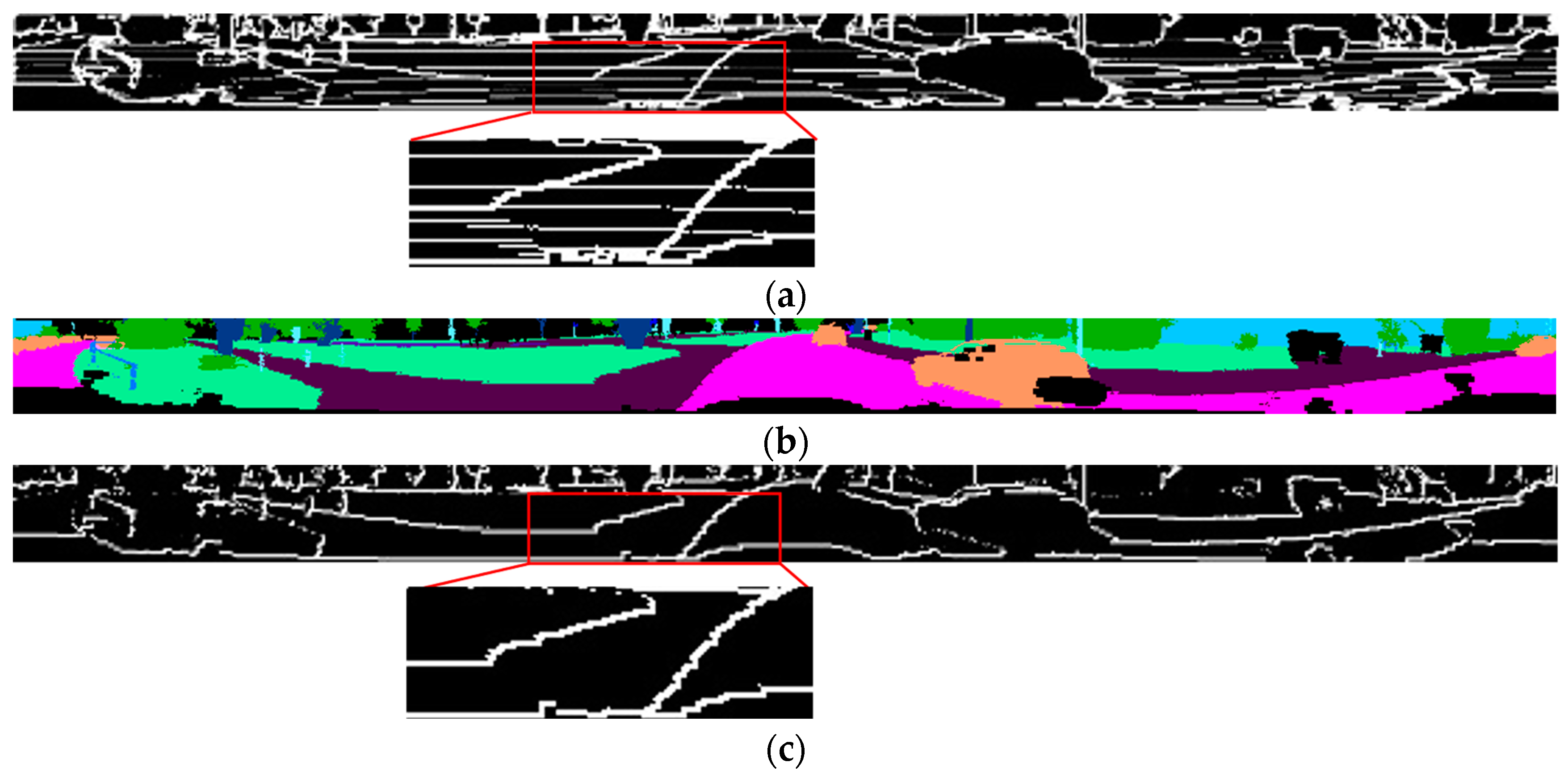
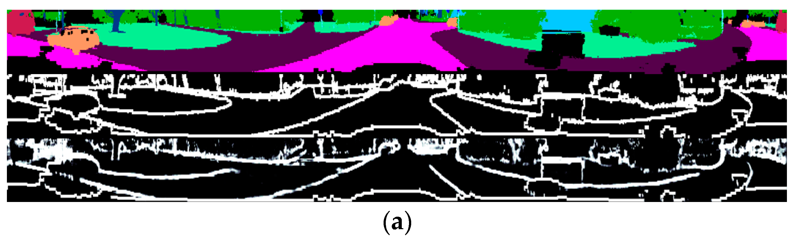
There are two outputs of the network, ground-truth (GT) semantic labels and GT binary edge labels. The GT edge labels, which is called edge map, are generated by the semantic labels. If a pixel has a neighbor with a different label, the pixel is designated as a border. During the pre-processing of labels, we notice that there are a lot of stripe patterns on the GT projection image, which is owed to the fact that the points in the point clouds do not cover all pixels of the image during the spherical projection, which affect the generation of edge map and thus the guidance of the segmentation results by edge features, as shown in Figure 3a. Therefore, we inpaint the image to determine the labels of the pixel points in the missing region, we first collect all pixels in the missing region using the morphological closing operation [42], and then we iterate each pixel and label it according to the class of its 8-direction neighboring pixels. Finally, a binary edge map that is not affected by the stripe patterns is obtained, as shown in Figure 3b,c. The difference between the edge maps before and after pre-processing is showcased in the enlarged parts of Figure 3a,c. The edges of terrain, sidewalk, and road are blurred by many stripe patterns in Figure 3a, while the edges are much clearer in Figure 3c.
3.3. Main Branch
In the main branch, the input of the network is a five-channel range image, where each pixel in the range image represents a point. Due to the superior spatial reconstruction capabilities of SalsaNext [28], we use its network structure, including ResContextBlock, ResBlock, and UpBlock, to acquire semantic information in the main branch, as shown in Figure 1. ResContextBlock and ResBlock contains a set of dilated convolutions to increase the receptive fields, whereas 1 × 1 convolution and residual connection are applied to enable the network to exploit more information from various depths in the receptive field. In UpBlock, the standard transpose convolution is replaced with a pixel-shuffle layer to avoid checkerboard artifacts caused by upsampling. Inspired by the idea of MLP from Point-Net [15] (using a multi-layer perceptron to make the point information redundant and thus obtain sufficient geometric information), we added three 1 × 1 convolutions before ResContextBlock to process the input to map each point to a higher dimensional space, as shown in Figure 1, which also enables the input to the edge segmentation module (ESM) to have more complete edge information.
3.4. Edge Segmentation Module
Low-level feature maps close to the input image have higher resolution but less semantic information than high-level feature maps. However, the latter obtain richer semantic information and larger receptive fields and can roughly predict most pixels of larger objects, but the limitation of resolution leads to problems such as blurry edges. Therefore, it is necessary to fuse high-resolution features from the bottom layer and high-level features from the top layer in the edge segmentation module (ESM).
The initial input of ESM comes from the low-level feature map of the main branch, as the high-resolution low-level feature maps provide more complete edge information, and then the edge features are gradually fused with high-level features.
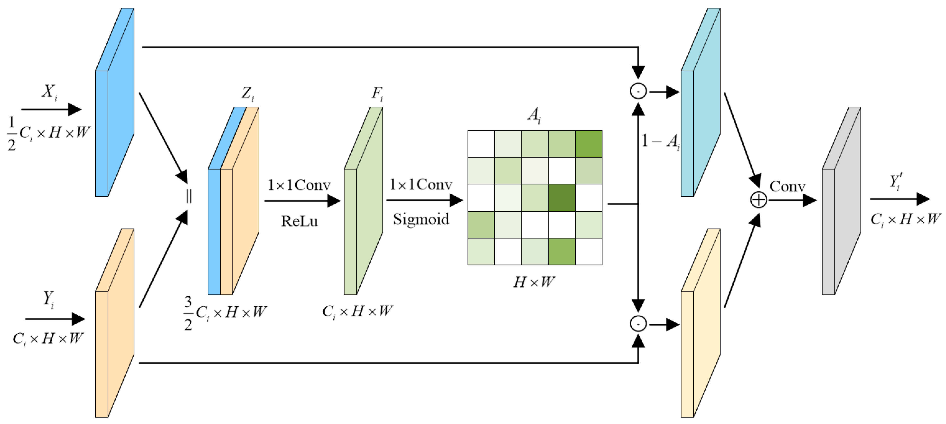
In ESM, we are more concerned with edge information, which is the shape features. However, a simple fusion of high-level and low-level features will mix in a lot of useless information (features that are not conducive to edge extraction). Therefore, we design three cascaded edge attention blocks (EABs) in ESM, as shown in Figure 4. This module is able to adaptively select the information relevant to the edges for processing while filtering out the rest of the useless information.
The output of the ESM has two roles, one for edge segmentation and the other for feature fusion with the main branch. For better-supervised edge segmentation, we generate edge maps from the GT semantic segmentation labels.
There are three EABs in the edge segmentation module, each EAB considers two inputs including the feature map from the main branch and feature map from the previous EAB, where and denote the channel numbers of and , respectively, and are the height and width of . is processed by a convolution layer and a Pixel-Shuffle layer to produce the upsampled feature maps and is processed by a convolution layer to generate the new feature maps , where represents the position of current EABs, is the channel numbers of , and are height and width of the feature map, respectively. We concatenate the two new feature maps to get and employ a convolution layer and a ReLu function on it to obtain the fusion feature . Then, is squeezed channel-wise to produce attention map , these operations can be defined as follows:
where , denotes the concatenation of feature maps, is convolution operations, and are the ReLu function and the Sigmoid function respectively.
Given the attention map , the output of the EAB is:
where denotes element-wise product operation and is the element-wise summation. If there is useful information in which is missing from to be fused into , will be small and will be large, so that the information can be passed over. Therefore, EAB can both guide the model’s attention to the right place and effectively suppress feature activation in unrelated areas. At the same time, it enhances the model representation capability without significantly increasing the model computation and the parameter number.
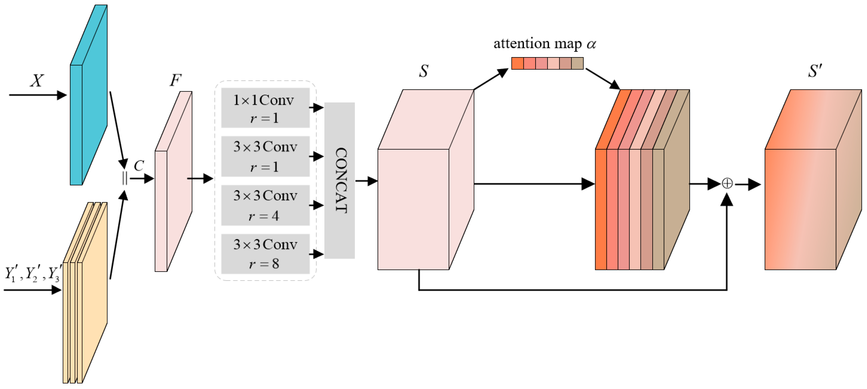
3.5. Edge Guided Fusion Module
The problem with the unstructured environment is unclear edges between classes, which still exists after converting the point clouds to range image. To alleviate this problem, we propose an edge guided fusion module (EGFM) to improve the discrimination of pixels around edges between two classes by fusing the edge-guided features from ESM with the features from the main branch., as shown in Figure 5. EGFM is a multi-scale fusion module based on channel attention, which can fuse the main branch features with sufficient semantic information and edge features with significant edge information, both of which can play a complementary role. During training, the GT edge map is an additional supervision to the learning process of edge features, and the learned multi-level edge features and the semantic features from the main branch are fed into EGFM for fusion; the output of EGFM is the predicted segmentation output.
The inputs to EGFM are the feature map of the last layer in the decoder and the concatenation of , , from three EABs in the edge segmentation module. The two inputs are concatenated together and fed into a convolution for fusion to obtain the feature map This process is formulated as:
Next, to capture richer multi-scale information, we use a four-branch ASPP to process the feature maps simultaneously. The first branch uses a convolution layer to extract features, keeping the receptive field unchanged, while branches 2–4 adopt dilated convolution with expansion rates of 1, 4, and 8, respectively. is obtained by concatenating the outputs of the four branches:
where represents the dilatation rate, means the convolution operation.
Then, the attention weights of each channel in the feature map are learned to emphasize the channels that contribute more to the segmentation result. The operation is as follows:
① Two pooling operations are conducted on the feature map. To aggregate the spatial features, average pooling and maximum pooling are used to compress the spatial information, thus two channel features are obtained;
② Two channel features are forwarded to a two-layer MLP, and to reduce parameters, the number of neurons in the first layer is set to . The weights of the two layers are shared;
③ Merge the two output features. Channel attention map is formulated as:
In this way, we end up with features that are semantically rich, while the edge details are well preserved.
3.6. Loss Function
Our network has two outputs, the segmentation labels and the edge labels. For semantic segmentation, the semantic loss Lseg is calculated by mixing the weighted cross-entropy loss and Lovász-Softmax loss [28]. The combination of weighted cross-entropy loss, a loss function designed for multi-classification problems with imbalanced samples, and Lovász-Softmax loss, a loss function that optimizes the semantic segmentation metric IOU (intersection over union) directly, results in more accurate network segmentation.
Similarly, for the edge loss, we also use binary weighted cross-entropy loss, written as:
where is the value of the -th position in the weight matrix, and and are the ground truth and predicted edge, respectively.
Inspired by Gated-SCNN [35], we expect that the whole network will be penalized more under the case of edge pixels being misclassified, thereby enhancing the guidance of the edge for the main branch segmentation, in the meantime, the consistency between the predicted edge and predicted semantic label can be ensured. Therefore, we use the loss function to describe the segmentation accuracy of the edge area:
where is the threshold of the positive edge, and are the ground truth and predicted label of the -th pixel of class . is set to 0.75 in our experiments.
Finally, the loss function of the overall network can be expressed as:
4. Experiments and Results
In this section, we first describe the dataset used for experiments, as well as the evaluation metrics commonly used in semantic segmentation, and present the implementation details of the experiments. Our method is then compared with the state-of-the-art methods in order to validate the effectiveness of the proposed edge-guided network. We also conduct ablation experiments for further analysis of the contribution of each module in our network.
4.1. Dataset and Metric
4.1.1. Dataset
The unstructured environments studied in this paper mainly include less structured rural environments and off-road environments, so we conducted experiments on two public datasets (SemanticKITTI dataset [43] including rural environments and RELLIS-3D dataset [44] for off-road environments) and our test dataset with less structured environments.
The SemanticKITTI dataset is a large-scale point clouds semantic segmentation dataset which captures numerous rural areas and roadway scenes in the medium-sized city of Karlsruhe by driving. The LiDAR used in this dataset is the Velodyne HDL-64E. We selected some rural scenes from the SemanticKITTI dataset as the test set. Experiments on the SemanticKITTI dataset will not only validate the segmentation performance of our method in a rural environment, but will also allow us to check its adaptability in different environments. We map “motorcyclist” to “motorcycle”, map “bicyclist” to “bicycle”, and map “other-ground” to “parking” based on the similarity of the classes and the balance between the number of corresponding point clouds.
The RELLIS-3D dataset is a dataset for semantic segmentation in off-road environments for autonomous driving. The dataset was collected at the Texas A&M University including the original 13,556 LiDAR scans, 6235 images, and their annotations, of which the LiDAR scans were divided into 7800/2413/3343 for the training, validation, and test sets, respectively. The LiDAR model is the 64-channel Ouster OS1.
To further prove the robustness of our method in different unstructured environments, we collected some unstructured scene data using the vehicle with a Robosense RS-LiDAR-M1 LiDAR as our test set and perform experiments on it.
4.1.2. Metric
We use the commonly used metrics intersection-over-union (IoU) and mean intersection-over-union (mIoU) over all classes to evaluate the performance of our method, defined as follows:
where , , and represent the number of true positive points, false positive points, and false negative points, respectively, denote the IoU of class , and indicates the number of classes.
4.2. Implementation Details
Our method is implemented on the PyTorch platform and run by a single GeForce RTX 3090 GPU with 24 G memory. The stochastic gradient descent (SGD) optimizer is used for optimization, and the momentum and weight decay parameters are set to 0.9 and 0.001, respectively. The initial learning rate is set to 0.01, and we trained the model for 150 epochs. Considering the limitation of GPU memory, the batch size is set to a fixed 8. The input size of the network is set to , and with this width and height setting, the generated range images are dense while retaining enough information. The GT edge labels are only used as additional supervision during model training and are not needed during testing, which facilitates realistic applications. Furthermore, we use the kNN-based post-processing method described in [26]. The post-processing step of back-projecting the range image to the point cloud is not involved in the training process, it is only used during the test process and when calculating the mIoU of our method. In addition, the pre-processing process is only used to generate accurate edge maps and does not change the range images or the GT projection images, therefore the calculation of test accuracy is not affected.
4.3. Experimental Results
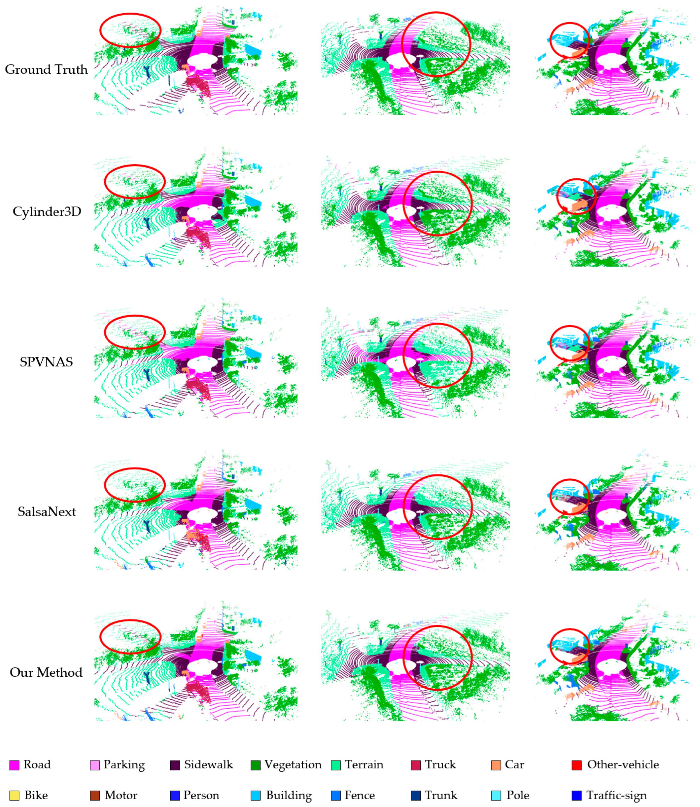
4.3.1. Experiment on SemanticKITTI Dataset
We compare our method with several state-of-the-art representative methods through the experiment on SemanticKITTI dataset, as shown in Table 1. The last two rows show the experimental results of the range-based method SalsaNext and our method, and the first to third rows show the results of RandLA-Net (point-based method), Cylinder3D (voxel-based method), and SPVNAS (point-voxel method), respectively. The results contain the IoU of each class, mIoU, and single frame prediction time (including data preprocessing time). Since the segmentation results of the drivable area and the static obstacles with large area in the unstructured environment have a greater impact on driving decisions, all classes are divided into two parts in the table, one containing road, parking, sidewalk, vegetation, and terrain, which account for 76.5% of the total point clouds, representing the drivable area, and the large static obstacles exist in the unstructured environment, and the other containing the remaining classes.
As shown in Table 1, our model achieves 68.02% mIoU, a 2.35% improvement over the current state-of-the-art range-based method, SalsaNext, while ensuring a real-time network performance of 35 ms per frame. Our network outperforms SalsaNext in segmentation accuracy for both drivable areas and large static obstacles thanks to the guidance of the extracted edge features. For a comprehensive evaluation, we also compared our method with three other state-of-the-art methods. Our method outperforms RandLANet in both accuracy and real-time performance because our network preserves those key points lost in RandLANet and avoids the complex pre-processing in RandLANet. Cylinder3D and SPVNAS provide very good results in terms of segmentation accuracy since they are voxel-based and fusion-based methods, which can retain accurate spatial information very well. However, their higher mIoU mainly benefits from those obstacles that are uncommon in unstructured environments with a relatively small percentage (less than 23.5% in total) but rich in categories, such as car, bike, motor, pole, and traffic-sign, etc. In addition, these methods are computationally intensive and do not balance the trade-off between segmentation accuracy and real-time performance well, making them unsuitable for autonomous driving tasks. In contrast, our method provides competitive segmentation accuracy while maintaining the real-time performance of the network. In particular, thanks to the ESM module’s ability to retain high-resolution features, which provide more complete edge information, our model has a noticeable advantage in segmenting classes that rely on high-resolution edge features. While segmenting drivable areas such as road, parking, and sidewalk, and large static obstacles such as vegetation, which account for 76.5% of the overall point clouds, our segmentation results remains the best even when compared to those of Cylinder3D and SPVNAS.
We selected some samples from our experimental results and show the results of our model compared to other methods in Figure 6, in addition, the corresponding GT edge maps and predicted edge maps are provided in Figure A2 of Appendix B to showcase the result of the edge segmentation modules. The first row is the visualization of the ground truth of the three scenes, the last row is our predictions, and the other rows are the predictions of other networks. We use the red circles to mark challenging regions that are prone to mis-segmentation. In the first scene, our method can segment the edge of the sidewalk accurately, but SalsaNext does not identify this part of the feature due to a partial loss of features in the upsampling process. SPVNAS misclassifies the sidewalk, and Cylinder3D identification of the feature the edge segmentation was poor. In the second scene, our method outperforms the other methods in distinguishing between vegetation and terrain, because our edge-guided module uses edge features to optimize the segmentation inaccuracy caused by blurred class-to-class edges. Our method also achieves better segmentation for the building in the third scene compared to the other methods.
4.3.2. Experiment on RELLIS-3D Dataset
To verify the robustness of our method, we also compare it to baseline on the full test set in Appendix A.
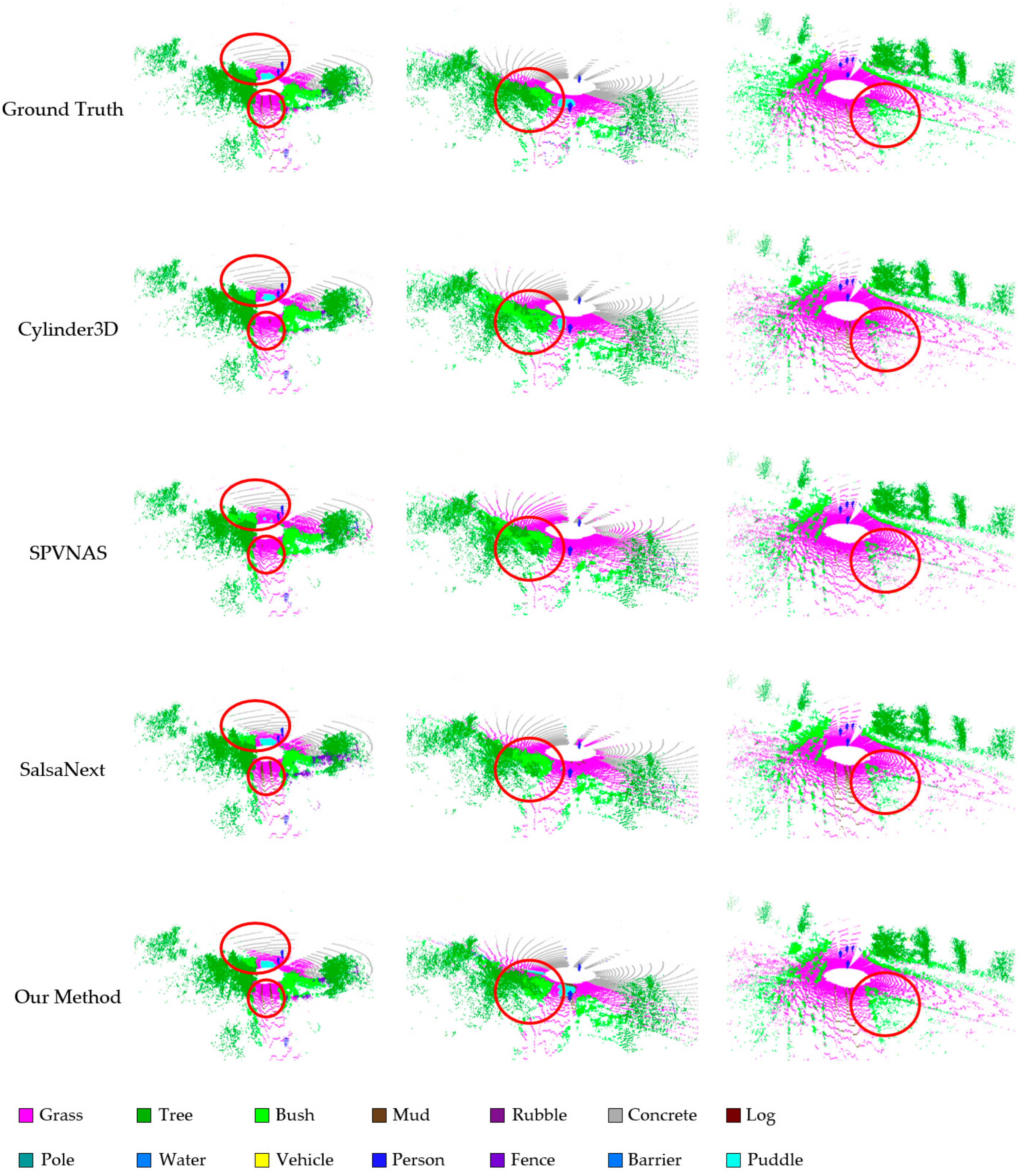
To further evaluate the effectiveness of the proposed method in an unstructured environment, we conducted experiments on the challenging off-road RELLIS-3D dataset. The results of our method compared to those of state-of-the-art methods are presented in Table 2. We group grass, tree, bush, mud, rubble, and concrete, which account for 96.8% of the total point clouds, into drivable areas and large static obstacles.
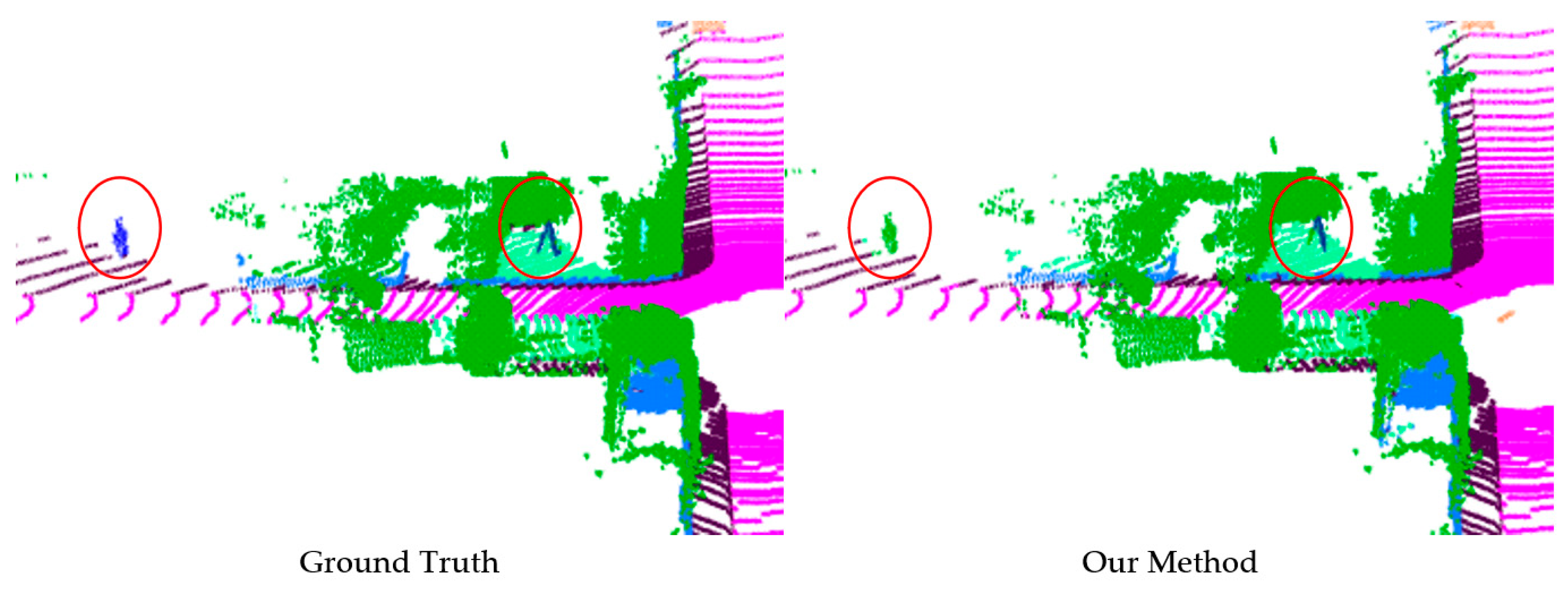
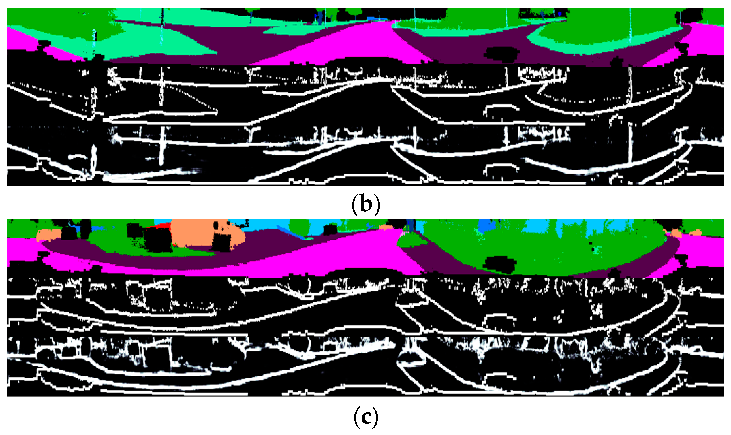
As shown in Table 2, our method achieves 43.88% mIoU, again the highest among range-based methods, with a 1.36% improvement compared to SalsaNext and guarantee real-time performance. When compared with other methods, our method outperforms RandLANet and SPVNAS in terms of accuracy and real-time performance. Cylinder3D achieves the best mIoU due to its cylindrical voxels that maintain the inherent properties of the point clouds, thus are more adaptable to the sparse-featured off-road scenes. However, its higher mIoU still benefits mainly from those obstacles that account for a very small proportion (less than 3.2% in total) but category-rich in the unstructured environment. In terms of real time, its inference time is 4.5 times that of our model. In particular, our method achieves the highest IoU when segmenting those classes that play a dominant role in the environment, such as grass and mud, which are drivable areas, with 1.22% and 2.3% improvement over Cylinder3D, respectively, and tree, bush, and rubble, which are large static obstacles, with 3.22%, 2.16%, and 4.5%. A sample selection of segmentation results is shown in Figure 7, in addition, the corresponding GT edge maps and predicted edge maps are provided in Figure A3 of Appendix B to showcase the result of the edge segmentation module.
4.3.3. Experiment on Our Real Vehicle Test Dataset
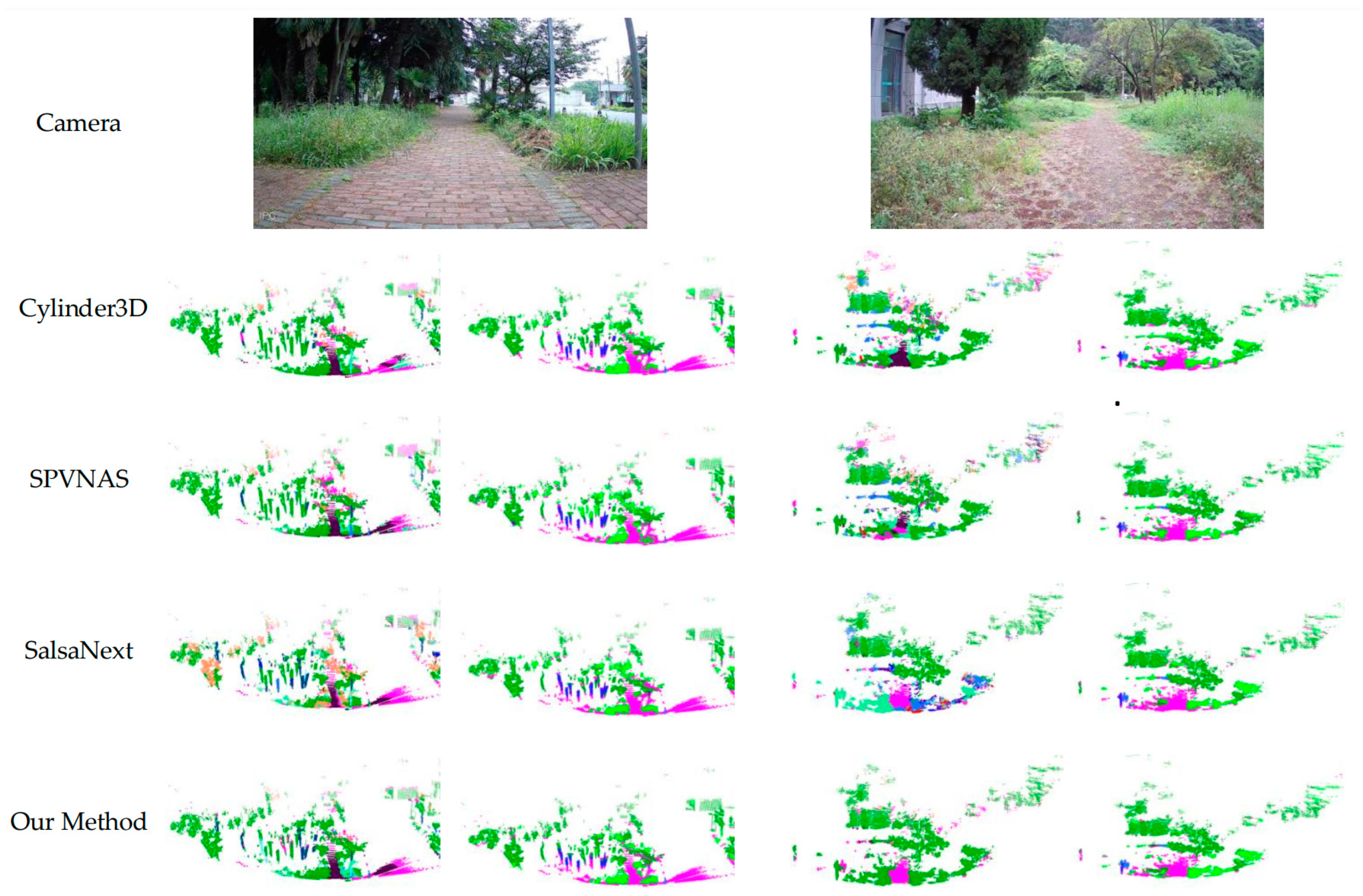
To demonstrate the robustness of our method in different unstructured environments, we also conducted experiments on an unstructured test set of our own collected data. Figure 8 shows the visualization results of our method and other different state-of-the-art methods. We select two scenes, the first one having relatively regular drivable areas and static obstacles, and the second one with more blurred class edges and more irregular geometric features of the classes compared to the first one. The first row of the figure shows the camera images, the first and third columns show the prediction results of the model trained with SemanticKITTI dataset, and the second and fourth columns show the prediction results of the model trained with Rellis-3D dataset. As can be seen, our network can segment the edges between classes more clearly and has better segmentation performance of drivable areas and static obstacles with large areas.
4.4. Ablation Study
An ablation study is performed on the RELLIS-3D dataset to evaluate the effectiveness for each module of our method. All training and testing environments were kept the same for each ablation experiment. We designed our ablation experiments by replacing or removing two key modules of the network. As shown in Table 3, (1) the baseline network only uses the main branch of our network; (2) we replace the EGFM with direct channel concatenation followed by a common convolutional layer for feature fusion; (3) we remove the ESM as well as the supervision of GT edge map and use the low-level features of the main branch as the second input to EGFM instead; (4) we remove the three 1 × 1 convolutions in main branch from our method.
Quantitative evaluation results in Table 3 shows that both modules have an advantage over the baseline performance because
- Using only ESM improves mIoU by 0.76% with 11.15 GFLOPs and 0.05 M parameters increasement compared to baseline;
- Using only EGFM improves mIoU by 0.21% with 17.75 GFLOPs and 0.07 M parameters increasement compared to baseline. Compared with only using the ESM, the performance improvement is not obvious. This is because the EGFM is based on the ESM and after the ESM is removed, the EGFM cannot fuse the edge features well;
- When combing the ESM and EGFM (our method), the mIoU is improved by 1.36% with 24.90 GFLOPs and 0.10 M parameters, an increase compared to the baseline, and performs much better than adding just one module alone as described above;
- When removing the three 1 × 1 convolutions from our method, the mIoU drop by 0.07%, but the FLOPs and parameters show only a minor decrease;
- The ablation experiments demonstrate the effectiveness of our designed modules and the effectiveness of using edge features to enhance semantic segmentation accuracy.
To further explore the role of the attention module in our proposed network, we investigate the effectiveness of the edge attention block (EAB) in ESM and the channel attention (CA) in EGFM. Specifically, for ESM without EAB, we replace the EAB with a convolutional layer, for EGFM without CA, we remove CA straight away. Corresponding results are shown in Table 4.
- With the removal of EAB and CA, the mIoU of our model decreased by 0.62% but is still 0.74% higher than the baseline, which proves the effectiveness of our overall edge-guided framework;
- By deleting only EAB, the mIoU of our model decreased by 0.45%, and after deleting only CA, the mIoU decreased by 0.21%, which indicates that EAB has a greater impact on the overall model than CA. We argue that the reason for this phenomenon lies in that, the absence of three cascading EABs can make the fused features contain too much unnecessary information, thus negatively affecting the response of CA, while CA does not affect the preceding EABs as it calibrates the fused features.
5. Discussion
Currently, semantic segmentation for unstructured environments is gradually receiving attention from researchers. We propose an edge-guided point clouds semantic segmentation network which can alleviate the problems of blurred class edges, thus improving the accuracy and adaptability of semantic segmentation for different unstructured environments. Extensive experimental results show that, our method outperforms other methods when segmenting drivable areas and large-area static obstacles that occupy a high proportion of the unstructured environment. This is because, on the one hand, our method is able to preserve high-resolution edge features and provide more complete edge detail information, and on the other hand, the additional supervision ensures consistency between the edge prediction results and the semantic segmentation results. Experiments have demonstrated the potentials of applying our method on semantic segmentation of the unstructured environments.
However, despite this, there are still areas where our work can be improved. The IoU of our method is not the best when it comes to segmenting some objects with richer 3D geometric information, such as car, person, trunk, and traffic-sign. It is because the range-based method loses some of the 3D spatial information. As shown in Figure 9, our method mis-segments the person and the trunk of the tree. Although these classes occupy a small proportion of the whole unstructured scene, it is sometimes crucial for scene understanding to segment them accurately. Therefore, our future work will focus on further optimizing the segmentation accuracy of these objects.
6. Conclusions
We propose a novel real-time LiDAR semantic segmentation network based on edge guidance for unstructured environments. The proposed method improves the overall segmentation performance by mining edge features through a supervised edge segmentation module in a multi-task learning manner. By designing the edge segmentation module (ESM) and the edge guided fusion module (EGFM), our network considers both edge information and semantic information. The ESM retains high-resolution features and provides more complete edge information for EGFM, while ensuring the consistency of edge prediction results and semantic segmentation results in a supervised manner. The EGFM module fuses the main branch features and edge features from ESM in a multi-scale manner. It improves the prediction accuracy of the model by mining the multi-scale features while emphasizing the channels that contribute to the segmentation results. Extensive experiments on SemanticKITTI dataset and RELLIS-3D dataset demonstrate the effectiveness and real-time performance of our method. In addition, our method achieves state-of-the-art results in segmenting drivable areas and large-area static obstacles that are particularly important for autonomous driving in unstructured environments. Also, the good performance of our method in our unstructured environment test dataset reflects its robustness. Furthermore, ablation experiments demonstrate the validity and reliability of each component of our proposed network.
Author Contributions
Conceptualization, X.L. and X.Y.; methodology, X.Y.; software, X.Y.; validation, X.Y. and P.N.; formal analysis, X.L. and Q.X.; investigation, X.Y.; resources, X.Y.; data curation, X.Y. P.N. and D.K.; writing—original draft preparation, X.Y.; writing—review and editing, X.L. X.Y. P.N. and D.K.; supervision, X.L. project administration, X.L. and Q.X.; funding acquisition, X.L. and Q.X. All authors have read and agreed to the published version of the manuscript.
Funding
This research was funded by the National Key R & D Program of China, grant number 2019YFC1511505, the National Natural Science Foundation of China, grant number 61973079 and the Primary Research & Development Plan of Jiangsu Province, grant number BE2022053-5.
Data Availability Statement
The SemanticKITTI Dataset used in this study is available at http://semantic-kitti.org/dataset.html (accessed on 13 May 2021); The RELLIS-3D Dataset used in this study is available at https://github.com/unmannedlab/RELLIS-3D (accessed on 8 January 2022).
Conflicts of Interest
The authors declare no conflict of interest.
Appendix A
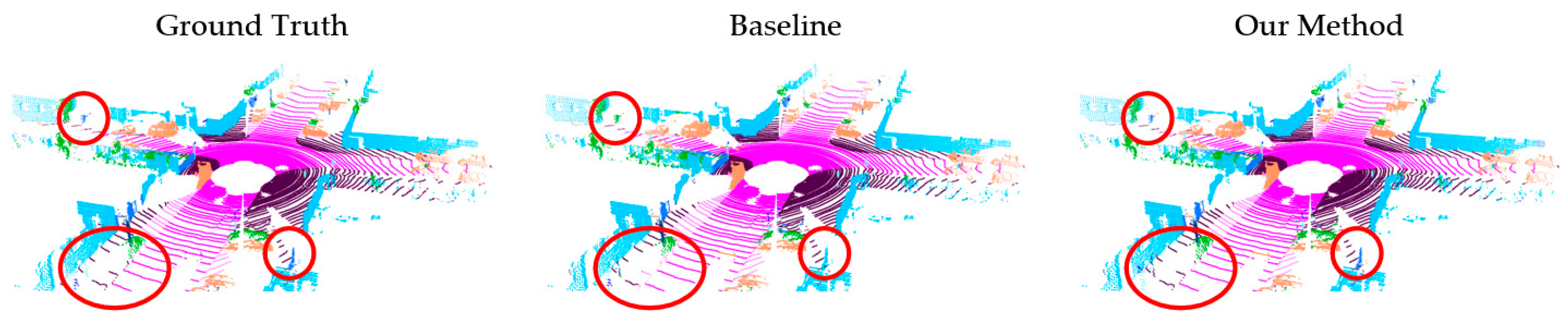
As shown in Table A1, our approach still achieves better results than baseline when using the full test dataset, which further verify the robustness of our method. In Figure A1, which is a sample of structured scenes, our method shows better segmentation accuracy than baseline on some fences and parts of sidewalks.

Table A1.
Comparison with baseline on the full test dataset.
| Methods | Time (ms) | mIoU (%) | Road | Parking | Sidewalk | Vegetation | Terrain | Truck | Car | Bike | Motor | Other-vehicle | Person | Building | Fence | Trunk | Pole | Traffic-sign |
|---|---|---|---|---|---|---|---|---|---|---|---|---|---|---|---|---|---|---|
| Baseline | 25 | 66.09 | 94.58 | 54.05 | 81.68 | 81.90 | 66.80 | 81.26 | 83.46 | 65.38 | 46.25 | 49.71 | 62.31 | 78.55 | 57.50 | 54.71 | 46.92 | 52.31 |
| ours | 35 | 68.59 | 95.20 | 58.51 | 82.14 | 82.31 | 66.83 | 87.26 | 84.54 | 70.14 | 48.68 | 47.20 | 61.49 | 82.15 | 60.37 | 59.72 | 59.44 | 51.49 |
The bolded parts indicate that the method has the best real-time performance or segmentation accuracy in the corresponding columns.
Figure A1.
Visual comparison with baseline on full test set.

Appendix B
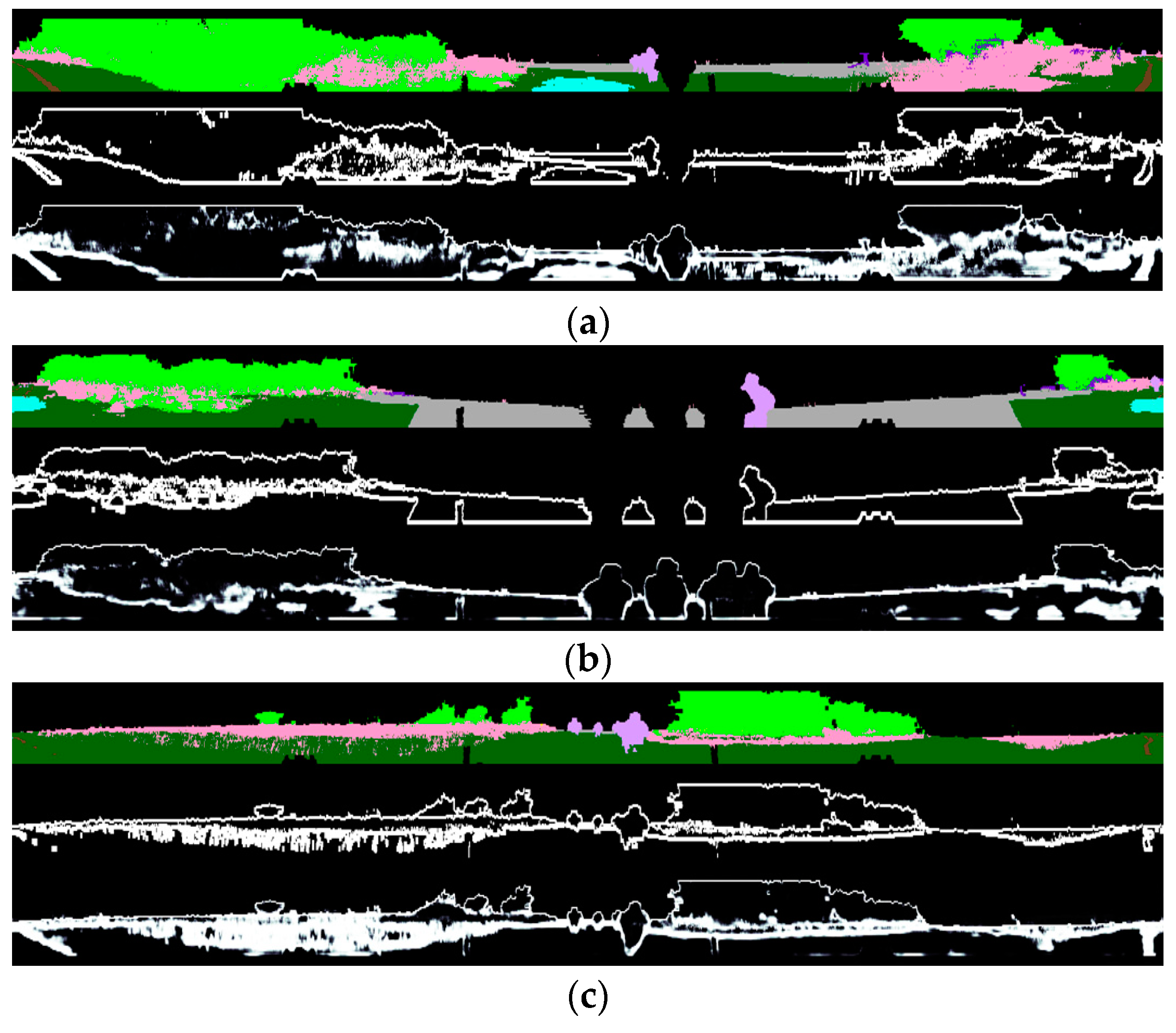
Figure A2.
The inpainted GT projection image (first row), GT edge maps (second row) and predicted edge maps (third row) of samples (a–c) from SemanticKITTI.
Figure A2.
The inpainted GT projection image (first row), GT edge maps (second row) and predicted edge maps (third row) of samples (a–c) from SemanticKITTI.


Figure A3.
The inpainted GT projection image (first row), GT edge maps (second row) and predicted edge maps (third row) of samples (a–c) from Rellis-3D.
Figure A3.
The inpainted GT projection image (first row), GT edge maps (second row) and predicted edge maps (third row) of samples (a–c) from Rellis-3D.

References
- He, Y.; Yu, H.; Liu, X.; Yang, Z.; Sun, W.; Wang, Y.; Fu, Q.; Zou, Y.; Mian, A. Deep learning based 3D segmentation: A survey. arXiv 2021, arXiv:2103.05423. [Google Scholar]
- Wang, W.; You, X.; Yang, J.; Su, M.; Zhang, L.; Yang, Z.; Kuang, Y. LiDAR-Based Real-Time Panoptic Segmentation via Spatiotemporal Sequential Data Fusion. Remote Sens. 2022, 14, 1775. [Google Scholar] [CrossRef]
- Feng, D.; Haase-Schütz, C.; Rosenbaum, L.; Hertlein, H.; Glaeser, C.; Timm, F.; Wiesbeck, W.; Dietmayer, K. Deep multi-modal object detection and semantic segmentation for autonomous driving: Datasets, methods, and challenges. IEEE Trans. Intell. Transp. Syst. 2020, 22, 1341–1360. [Google Scholar] [CrossRef] [Green Version]
- Zhao, L.; Xu, S.; Liu, L.; Ming, D.; Tao, W. SVASeg: Sparse Voxel-Based Attention for 3D LiDAR Point Cloud Semantic Segmentation. Remote Sens. 2022, 14, 4471. [Google Scholar] [CrossRef]
- Asgari Taghanaki, S.; Abhishek, K.; Cohen, J.P.; Cohen-Adad, J.; Hamarneh, G. Deep semantic segmentation of natural and medical images: A review. Artif. Intell. Rev. 2021, 54, 137–178. [Google Scholar] [CrossRef]
- Yang, R.; Yu, Y. Artificial convolutional neural network in object detection and semantic segmentation for medical imaging analysis. Front. Oncol. 2021, 11, 638182. [Google Scholar] [CrossRef]
- Li, Y.; Ma, L.; Zhong, Z.; Liu, F.; Chapman, M.A.; Cao, D.; Li, J. Deep learning for lidar point clouds in autonomous driving: A review. IEEE Trans. Neural Netw. Learn. Syst. 2020, 32, 3412–3432. [Google Scholar] [CrossRef]
- Guo, Z.; Huang, Y.; Hu, X.; Wei, H.; Zhao, B. A survey on deep learning based approaches for scene understanding in autonomous driving. Electronics 2021, 10, 471. [Google Scholar] [CrossRef]
- Baheti, B.; Innani, S.; Gajre, S.; Talbar, S. Semantic scene segmentation in unstructured environment with modified DeepLabV3+. Pattern Recognit. Lett. 2020, 138, 223–229. [Google Scholar] [CrossRef]
- Liu, H.; Yao, M.; Xiao, X.; Cui, H. A hybrid attention semantic segmentation network for unstructured terrain on Mars. Acta Astronaut. 2022, in press. [Google Scholar] [CrossRef]
- Gao, B.; Xu, A.; Pan, Y.; Zhao, X.; Yao, W.; Zhao, H. Off-road drivable area extraction using 3D LiDAR data. In Proceedings of the 2019 IEEE Intelligent Vehicles Symposium (IV), Paris, France, 9–12 June 2019; pp. 1505–1511. [Google Scholar]
- Zhu, Z.; Li, X.; Xu, J.; Yuan, J.; Tao, J. Unstructured road segmentation based on road boundary enhancement point-cylinder network using LiDAR sensor. Remote Sens. 2021, 13, 495. [Google Scholar] [CrossRef]
- Chen, Y.; Xiong, Y.; Zhang, B.; Zhou, J.; Zhang, Q. 3D point cloud semantic segmentation toward large-scale unstructured agricultural scene classification. Comput. Electron. Agric. 2021, 190, 106445. [Google Scholar] [CrossRef]
- Wei, H.; Xu, E.; Zhang, J.; Meng, Y.; Wei, J.; Dong, Z.; Li, Z. BushNet: Effective semantic segmentation of bush in large-scale point clouds. Comput. Electron. Agric. 2022, 193, 106653. [Google Scholar] [CrossRef]
- Qi, C.R.; Su, H.; Mo, K.; Guibas, L.J. Pointnet: Deep learning on point sets for 3d classification and segmentation. In Proceedings of the IEEE Conference on Computer Vision and Pattern Recognition, Honolulu, HI, USA, 21–26 July 2017; pp. 652–660. [Google Scholar]
- Qi, C.R.; Yi, L.; Su, H.; Guibas, L.J. Pointnet++: Deep hierarchical feature learning on point sets in a metric space. Adv. Neural Inf. Process. Syst. 2017, 30. [Google Scholar] [CrossRef]
- Thomas, H.; Qi, C.R.; Deschaud, J.-E.; Marcotegui, B.; Goulette, F.; Guibas, L.J. Kpconv: Flexible and deformable convolution for point clouds. In Proceedings of the IEEE/CVF International Conference on Computer Vision, Seoul, Republic of Korea, 27 October–2 November 2019; pp. 6411–6420. [Google Scholar]
- Hu, Q.; Yang, B.; Xie, L.; Rosa, S.; Guo, Y.; Wang, Z.; Trigoni, N.; Markham, A. Randla-net: Efficient semantic segmentation of large-scale point clouds. In Proceedings of the IEEE/CVF Conference on Computer Vision and Pattern Recognition, Seattle, WA, USA, 13–19 June 2020; pp. 11108–11117. [Google Scholar]
- Maturana, D.; Scherer, S. Voxnet: A 3d convolutional neural network for real-time object recognition. In Proceedings of the 2015 IEEE/RSJ International Conference on Intelligent Robots and Systems (IROS), Hamburg, Germany, 28 September–3 October 2015; pp. 922–928. [Google Scholar]
- Zhou, Y.; Tuzel, O. Voxelnet: End-to-end learning for point cloud based 3d object detection. In Proceedings of the IEEE Conference on Computer Vision and Pattern Recognition, Salt Lake City, UT, USA, 18–23 June 2018; pp. 4490–4499. [Google Scholar]
- Tang, H.; Liu, Z.; Zhao, S.; Lin, Y.; Lin, J.; Wang, H.; Han, S. Searching efficient 3d architectures with sparse point-voxel convolution. In Proceedings of the European Conference on Computer Vision, Glasgow, UK, 23–28 August 2020; pp. 685–702. [Google Scholar]
- Zhou, H.; Zhu, X.; Song, X.; Ma, Y.; Wang, Z.; Li, H.; Lin, D. Cylinder3d: An effective 3d framework for driving-scene lidar semantic segmentation. arXiv 2020, arXiv:2008.01550. [Google Scholar]
- Vosselman, G.; Gorte, B.G.; Sithole, G.; Rabbani, T. Recognising structure in laser scanner point clouds. Int. Arch. Photogramm. Remote Sens. Spat. Inf. Sci. 2004, 46, 33–38. [Google Scholar]
- Wu, B.; Wan, A.; Yue, X.; Keutzer, K. Squeezeseg: Convolutional neural nets with recurrent crf for real-time road-object segmentation from 3d lidar point cloud. In Proceedings of the 2018 IEEE International Conference on Robotics and Automation (ICRA), Brisbane, Australia, 21–25 May 2018; pp. 1887–1893. [Google Scholar]
- Wu, B.; Zhou, X.; Zhao, S.; Yue, X.; Keutzer, K. Squeezesegv2: Improved model structure and unsupervised domain adaptation for road-object segmentation from a lidar point cloud. In Proceedings of the 2019 International Conference on Robotics and Automation (ICRA), Montreal, QC, Canada, 20–24 May 2019; pp. 4376–4382. [Google Scholar]
- Milioto, A.; Vizzo, I.; Behley, J.; Stachniss, C. Rangenet++: Fast and accurate lidar semantic segmentation. In Proceedings of the 2019 IEEE/RSJ International Conference on Intelligent Robots and Systems (IROS), Macau, China, 4–8 November 2019; pp. 4213–4220. [Google Scholar]
- Kochanov, D.; Nejadasl, F.K.; Booij, O. Kprnet: Improving projection-based lidar semantic segmentation. arXiv 2020, arXiv:2007.12668. [Google Scholar]
- Cortinhal, T.; Tzelepis, G.; Erdal Aksoy, E. SalsaNext: Fast, uncertainty-aware semantic segmentation of LiDAR point clouds. In Proceedings of the International Symposium on Visual Computing, San Diego, CA, USA, 5–7 October 2020; pp. 207–222. [Google Scholar]
- Liu, T.; Liu, D.; Yang, Y.; Chen, Z. Lidar-based traversable region detection in off-road environment. In Proceedings of the 2019 Chinese Control Conference (CCC), Guangzhou, China, 27–30 July 2019; pp. 4548–4553. [Google Scholar]
- Chen, L.; Yang, J.; Kong, H. Lidar-histogram for fast road and obstacle detection. In Proceedings of the 2017 IEEE International Conference on Robotics and Automation (ICRA), Singapore, 29 May–3 June 2017; pp. 1343–1348. [Google Scholar]
- Bertasius, G.; Shi, J.; Torresani, L. Semantic segmentation with boundary neural fields. In Proceedings of the IEEE Conference on Computer Vision and Pattern Recognition, Las Vegas, NV, USA, 27–30 June 2016; pp. 3602–3610. [Google Scholar]
- Chen, L.-C.; Papandreou, G.; Kokkinos, I.; Murphy, K.; Yuille, A.L. Deeplab: Semantic image segmentation with deep convolutional nets, atrous convolution, and fully connected crfs. IEEE Trans. Pattern Anal. Mach. Intell. 2017, 40, 834–848. [Google Scholar] [CrossRef] [Green Version]
- Peng, C.; Zhang, X.; Yu, G.; Luo, G.; Sun, J. Large kernel matters--improve semantic segmentation by global convolutional network. In Proceedings of the IEEE Conference on Computer Vision and Pattern Recognition, Honolulu, HI, USA, 21–26 July 2017; pp. 4353–4361. [Google Scholar]
- Yu, C.; Wang, J.; Peng, C.; Gao, C.; Yu, G.; Sang, N. Learning a discriminative feature network for semantic segmentation. In Proceedings of the IEEE Conference on Computer Vision and Pattern Recognition, Salt Lake City, UT, USA, 18–23 June 2018; pp. 1857–1866. [Google Scholar]
- Takikawa, T.; Acuna, D.; Jampani, V.; Fidler, S. Gated-scnn: Gated shape cnns for semantic segmentation. In Proceedings of the IEEE/CVF International Conference on Computer Vision, Seoul, Republic of Korea, 27 October–2 November 2019; pp. 5229–5238. [Google Scholar]
- Ma, H.; Yang, H.; Huang, D. Boundary Guided Context Aggregation for Semantic Segmentation. arXiv 2021, arXiv:2110.14587. [Google Scholar]
- Gong, J.; Xu, J.; Tan, X.; Zhou, J.; Qu, Y.; Xie, Y.; Ma, L. Boundary-aware geometric encoding for semantic segmentation of point clouds. In Proceedings of the AAAI Conference on Artificial Intelligence, Vancouver, BC, Canada, 2–9 February 2021; pp. 1424–1432. [Google Scholar]
- Hu, Z.; Zhen, M.; Bai, X.; Fu, H.; Tai, C.-L. Jsenet: Joint semantic segmentation and edge detection network for 3d point clouds. In Proceedings of the Computer Vision–ECCV 2020: 16th European Conference, Glasgow, UK, 23–28 August 2020; Part XX 16. pp. 222–239. [Google Scholar]
- Hao, F.; Li, J.; Song, R.; Li, Y.; Cao, K. Mixed Feature Prediction on Boundary Learning for Point Cloud Semantic Segmentation. Remote Sens. 2022, 14, 4757. [Google Scholar] [CrossRef]
- Armeni, I.; Sener, O.; Zamir, A.R.; Jiang, H.; Brilakis, I.; Fischer, M.; Savarese, S. 3d semantic parsing of large-scale indoor spaces. In Proceedings of the IEEE Conference on Computer Vision and Pattern Recognition, Las Vegas, NV, USA, 27–30 2016; pp. 1534–1543. [Google Scholar]
- Dai, A.; Chang, A.X.; Savva, M.; Halber, M.; Funkhouser, T.; Nießner, M. Scannet: Richly-annotated 3d reconstructions of indoor scenes. In Proceedings of the IEEE Conference on Computer Vision and Pattern Recognition, Honolulu, HI, USA, 21–26 July 2017; pp. 5828–5839. [Google Scholar]
- Haralick, R.M.; Sternberg, S.R.; Zhuang, X. Image analysis using mathematical morphology. IEEE Trans. Pattern Anal. Mach. Intell. 1987, PAMI-9, 532–550. [Google Scholar] [CrossRef] [PubMed]
- Behley, J.; Garbade, M.; Milioto, A.; Quenzel, J.; Behnke, S.; Stachniss, C.; Gall, J. Semantickitti: A dataset for semantic scene understanding of lidar sequences. In Proceedings of the IEEE/CVF International Conference on Computer Vision, Seoul, Republic of Korea, 27 October–2 November 2019; pp. 9297–9307. [Google Scholar]
- Jiang, P.; Osteen, P.; Wigness, M.; Saripalli, S. Rellis-3d dataset: Data, benchmarks and analysis. In Proceedings of the 2021 IEEE International Conference on Robotics and Automation (ICRA), Xi’an, China, 30 May–5 June 2021; pp. 1110–1116. [Google Scholar]
Figure 1.
The architecture of our network.

Figure 2.
LiDRA projection. (a) Original point clouds with ground truth labels; (b) Projected ground truth labels.
Figure 2.
LiDRA projection. (a) Original point clouds with ground truth labels; (b) Projected ground truth labels.


Figure 3.
Process of making an edge map. (a) Edge map affected by the stripe patterns; (b) Inpainted GT semantic labels; (c) Edge map unaffected by the stripe patterns.
Figure 3.
Process of making an edge map. (a) Edge map affected by the stripe patterns; (b) Inpainted GT semantic labels; (c) Edge map unaffected by the stripe patterns.

Figure 4.
The Edge Attention Block (EAB).

Figure 5.
The edge guided fusion module (EGFM).

Figure 6.
Visual comparison with different state-of-the-art methods on the Semantic KITTI dataset.

Figure 7.
Visual comparison with different state-of-the-art methods on RELLIS-3D dataset.

Figure 8.
Visual comparison with different state-of-the-art methods on our unstructured test dataset.
Figure 8.
Visual comparison with different state-of-the-art methods on our unstructured test dataset.

Figure 9.
A false segmentation case of person and trunks.

Table 1.
Comparisons with state-of-the-art methods on the SemanticKITTI dataset.
| Methods | Time (ms) | mIoU (%) | Road | Parking | Sidewalk | Vegetation | Terrain | Truck | Car | Bike | Motor | Other-vehicle | Person | Building | Fence | Trunk | Pole | Traffic-sign |
|---|---|---|---|---|---|---|---|---|---|---|---|---|---|---|---|---|---|---|
| RandLANet | 639 | 60.99 | 91.44 | 42.21 | 76.50 | 84.19 | 73.63 | 67.74 | 93.07 | 65.74 | 20.64 | 41.46 | 48.79 | 85.55 | 38.86 | 58.49 | 51.63 | 36.05 |
| Cylinder3D | 157 | 69.57 | 93.21 | 41.38 | 79.63 | 83.92 | 63.09 | 75.44 | 95.46 | 75.29 | 53.01 | 44.96 | 73.35 | 90.68 | 60.96 | 67.57 | 65.43 | 49.71 |
| SPVNAS | 173 | 69.05 | 91.77 | 43.52 | 74.95 | 85.61 | 63.75 | 82.42 | 96.09 | 81.69 | 40.31 | 62.87 | 65.29 | 88.91 | 56.76 | 61.54 | 60.87 | 48.46 |
| SalsaNext | 25 | 65.67 | 93.28 | 38.93 | 79.22 | 83.85 | 69.67 | 66.61 | 91.92 | 79.67 | 37.49 | 45.57 | 66.73 | 85.2 | 48.43 | 60.31 | 56.62 | 47.24 |
| ours | 35 | 68.02 | 94.41 | 44.96 | 80.97 | 85.67 | 70.04 | 88.67 | 92.12 | 80.44 | 44.53 | 39.5 | 60.74 | 86.12 | 51.36 | 63.29 | 60.78 | 44.72 |
The bolded parts indicate that the method has the best real-time performance or segmentation accuracy in the corresponding columns.
Table 2.
Comparisons with state-of-the-art methods on the RELLIS-3D dataset.
| Methods | Time (ms) | mIoU | Grass | Tree | Bush | Mud | Rubble | Concrete | Log | Pole | Water | Vehicle | Person | Fence | Barrier | Puddle |
|---|---|---|---|---|---|---|---|---|---|---|---|---|---|---|---|---|
| RandLANet | 633 | 38.61 | 62.11 | 76.72 | 69.82 | 8.46 | 1.72 | 72.83 | 6.29 | 42.78 | 0 | 34.75 | 82.89 | 10.23 | 54.25 | 17.63 |
| Cylinder3D | 149 | 45.61 | 64.92 | 76.51 | 71.77 | 10.62 | 2.28 | 80.42 | 5.49 | 63.78 | 0 | 50.31 | 87.03 | 11.81 | 80.53 | 33.04 |
| SPVNAS | 168 | 42.68 | 64.12 | 76.06 | 71.51 | 8.54 | 5.23 | 70.01 | 15.05 | 54.43 | 0 | 48.57 | 85.79 | 10.99 | 64.81 | 22.44 |
| SalsaNext | 25 | 42.52 | 65.34 | 79.64 | 73.59 | 11.58 | 6.61 | 77.87 | 22.17 | 44.26 | 0 | 26.62 | 84.41 | 13.53 | 63.69 | 26.02 |
| ours | 35 | 43.88 | 66.14 | 79.73 | 73.93 | 12.92 | 6.78 | 77.15 | 22.42 | 48.9 | 0 | 27.9 | 84.32 | 13.27 | 77.23 | 23.67 |
The bolded parts indicate that the method has the best real-time performance or segmentation accuracy in the corresponding columns.
Table 3.
Quantitative evaluation of ablation studies on the RELLIS-3D dataset.
| Module | Time (ms) | mIoU (%) | FLOPs (G) | Parameters (M) | ||
|---|---|---|---|---|---|---|
| Baseline | ESM | EGFM | ||||
| ✓ | 25 | 42.52 | 121.01 | 6.69 | ||
| ✓ | ✓ | 29 | 43.28 | 132.16 | 6.74 | |
| ✓ | ✓ | 33 | 42.73 | 138.75 | 6.76 | |
| ✓ | ✓ | ✓ | 35 | 43.88 | 145.91 | 6.79 |
| ✓ * | ✓ | ✓ | 34 | 43.81 | 145.26 | 6.78 |
* w/o three 1 × 1 convolutions in main branch.
Table 4.
Results of the effect of attention module on segmentation performance.
| Baseline | ESM Type | EGFM Type | mIoU (%) |
|---|---|---|---|
| ✓ | w/o EAB | w/o CA | 43.26 |
| ✓ | w/o EAB | w/CA | 43.43 |
| ✓ | w/EAB | w/o CA | 43.67 |
| ✓ | w/EAB | w/CA | 43.88 |
Disclaimer/Publisher’s Note: The statements, opinions and data contained in all publications are solely those of the individual author(s) and contributor(s) and not of MDPI and/or the editor(s). MDPI and/or the editor(s) disclaim responsibility for any injury to people or property resulting from any ideas, methods, instructions or products referred to in the content. |
© 2023 by the authors. Licensee MDPI, Basel, Switzerland. This article is an open access article distributed under the terms and conditions of the Creative Commons Attribution (CC BY) license (https://creativecommons.org/licenses/by/4.0/).
Share and Cite
MDPI and ACS Style
Yin, X.; Li, X.; Ni, P.; Xu, Q.; Kong, D. A Novel Real-Time Edge-Guided LiDAR Semantic Segmentation Network for Unstructured Environments. Remote Sens. 2023, 15, 1093. https://doi.org/10.3390/rs15041093
AMA Style
Yin X, Li X, Ni P, Xu Q, Kong D. A Novel Real-Time Edge-Guided LiDAR Semantic Segmentation Network for Unstructured Environments. Remote Sensing. 2023; 15(4):1093. https://doi.org/10.3390/rs15041093
Chicago/Turabian StyleYin, Xiaoqing, Xu Li, Peizhou Ni, Qimin Xu, and Dong Kong. 2023. "A Novel Real-Time Edge-Guided LiDAR Semantic Segmentation Network for Unstructured Environments" Remote Sensing 15, no. 4: 1093. https://doi.org/10.3390/rs15041093
Note that from the first issue of 2016, this journal uses article numbers instead of page numbers. See further details here.