
Characterizing Coastal Wind Speed and Significant Wave Height Using Satellite Altimetry and Buoy Data


Department of Civil and Environmental Engineering, School of Engineering, University of Connecticut, Storrs, CT 06269, USA
*
Author to whom correspondence should be addressed.
Remote Sens. 2023, 15(4), 987; https://doi.org/10.3390/rs15040987
Submission received: 3 December 2022
/
Revised: 5 February 2023
/
Accepted: 7 February 2023
/
Published: 10 February 2023
(This article belongs to the Special Issue Coastal Area Observations Based on Satellite Altimetry Data)
Abstract
:Wind speed and significant wave height are the most relevant metocean variables that support a wide range of engineering and economic activities. Their characterization through remote sensing estimations is required to compensate for the shortage of in situ observations. This study demonstrates the value of satellite altimetry to identify typical spatial patterns of wind speed and significant wave height in the northeastern region of the United States. Data from five altimetry satellite missions were evaluated against the available in situ observations with a 10 km sampling radius and a 30 min time window. An objective analysis of the collective altimeter dataset was performed to create aggregated composite maps of the wind speed and significant wave height. This asynchronous compositing of multi-mission altimeter data is introduced to compile a sufficient sampling of overpasses over the area of interest. The results of this approach allow for quantifying spatial patterns for the wind speed and significant wave height in the summer and winter seasons. The quality of altimeter estimations was assessed regarding the distance from the coast and the topography. It was found that while the altimeter data are highly accurate for the two variables, bias increases near the coast. The average minimum and maximum wind speed values detected in buoy stations less than 40 km from the coast were not matched by the aggregated altimeter time series. The method exposes the spatial and time gaps to be filled using data from future missions. The challenges of the objective analysis near the coast, especially in semi-enclosed areas, and the implications of the altimeter estimations due to the land contamination are explained. The results indicate that the combination of altimetry data from multiple satellite missions provides a significant complementary information resource for nearshore and coastal wind and wave regime estimations.
1. Introduction
Wind and wave conditions are two of the leading environmental factors connected to our capacity for the sustainable exploitation of offshore wind. Specifically, their accurate estimation is an essential information resource for ship routing, coastal engineering, and several other coastal activities. The developing offshore wind energy industry needs these estimations for prospecting and ensuring the optimal siting of wind farms. Besides, real-time monitoring of wind and waves for decision-making is vital during the wind farms’ construction, operation, and decommissioning. Satellite radar altimeters have played a pivotal role in the global observation of ocean surface wind speed (WS) and significant wave height (SWH) for the past three decades. Numerical models and in situ observations from a network of buoys also support offshore wind energy with the characterization of these conditions [1].
This study’s motivation originates from the rapid rise of offshore wind developments on the United States East Coast in recent years. It focuses on the Northeast US wind and wave regime’s characterization using in situ observations from buoys moored in the domain and satellite altimetry data. Although their measurements are limited to only specific regions, the in situ data from the widely recognized National Data Buoy Center (NDBC) and Coastal Data Information Program (CDIP) extended network of stations are considered closer to the ground truth than the remote sensing observations. In situ observations combined with model outputs provide a powerful method to calibrate and validate altimeter observations [2]. However, the data from buoys are of significant importance, particularly near the coast and small domains. Their advantage relies upon providing a long-term, reliable, and quality-controlled time-series record, rendering them suitable for accurately estimating the WS and SWH normal conditions. On the other hand, they represent measurements in point locations; hence, spatial gaps exist in the analyzed conditions. Increasing observations from multiple satellite altimeters can potentially fill these spatial gaps. While a sprawl of data from various remote sensing capabilities, including the next generation of satellite altimeter data, is growing, their use is more effective when combined with buoy measurements. The disadvantage of the satellite altimeters is the low temporal resolution, as it depends on each mission’s cycle.
The satellite altimetry’s contributions to the global wind–wave characterization and the challenges for future missions have been well-documented [3]. However, the altimeter observations’ spatiotemporal gaps and the reduced accuracy in the first 20–30 km offshore imply the need for higher spatial resolution and additional future altimeter missions, as well as synergy with other types of wind and wave remote sensing capabilities. Still, studies on the long-term global calibration and validation of the different generations of satellite altimeters against buoy data have classified both the WS and SWH information as high quality, which can also be utilized for climate projections [4]. On the other hand, the altimeters’ low temporal resolution and the fact that the overpasses’ timing for certain altimeter missions is almost constant at every cycle impede resolving the WS diurnal variability. At the same time, the dependence of the WS estimations on the atmospheric stability induces an additional error source [5]. An intercomparison between the current generation’s altimeter missions in coastal regions has confirmed that the WS is consistent. In most intercomparison studies, the WS and SWH observations from different altimeter missions are consistent. However, the results from studies focused on small regions surrounded by land have indicated discrepancies in the intercomparison of SWH, which might be dependent on the study area [6]. Another factor affecting the altimeter observations’ quality in the coastal zone is the direction of each altimeter track. The results from previous studies have indicated that the measurements from the tracks with directions toward the coast are generally less influenced by land interference than the tracks passing over the land and moving in an offshore direction [7]. Evaluating the WS and SWH altimeter observations near the coast has been challenging due to the reduced altimeter accuracy but also avoiding the altimeter signal’s land interference and the topography’s influence when matching with buoy stations [8]. Although its spatial resolution is still low, properly combining the multi-mission satellite altimeter datasets to characterize the WS and SWH spatial variability in coastal regions where there is a shortage of in situ observations is valuable as prior estimated values for offshore applications [9].
Most studies neglect the altimeter data in the first 50 km offshore, owing to the challenges of coastal altimetry, specifically the land contamination of the altimeter waveform and the poor matching with buoy observations due to the topography impact. Therefore, an evaluation of the WS and SWH altimeter observations near the US Northeast coast at a regional level has not been addressed. Furthermore, there is a growing demand for accurately estimating the WS and SWH spatial variability and gradients for decision-making due to the absence of a dense network of offshore in situ stations. Recent studies focused on resource characterization using Synthetic Aperture Radar (SAR) observations [10] have introduced an alternative approach to quantifying and illustrating the coastal WS variability and gradients. However, the uneven sampling of SAR data throughout the year and the WS measurements at a specific time during the day restricted estimating the seasonal and diurnal variability, while the performance of SAR near the coast is uncertain. Moreover, predicting and quantifying the errors associated with the interpolated maps, along with instrumental and sampling errors, has been limited.
The present study describes the WS diurnal variability for the domain of interest based on buoy data. The WS and SWH accuracy of the current generation of altimeters is quantified by evaluating the buoy–altimeter discrepancies near the coast using a reduced sampling radius. The WS and SWH seasonal variability and spatial gradients are characterized based on multi-mission altimeter data composites using a more extended time window and evaluated based on the buoy data. Finally, the errors in estimating the altimeter time composite values are examined as data from the additional altimeter missions are added to the estimations and the limitations of demonstrating the WS diurnal variability based on a multi-mission altimeter dataset are explained.
2. Materials and Methods
Characterizing the WS and SWH at a regional level dictates the use of data from multiple altimeter missions. The approach described herein includes creating a multi-mission altimetry dataset that will first be evaluated based on the in situ observations from buoys and then utilize the collective altimetry dataset to identify the wind and wave dominant features on a regional level and multiple time scales of variability. The altimetry validation method against the buoy observations described in the section was selected based on widely recognized techniques in the literature [11] but also considering the inherent challenges of coastal altimetry, such as the distance of the buoy stations from the coast and the topography of the domain of interest [8]. Since a numerical model output was not used in this study, the Kriging interpolation of the altimeter data was selected for producing the maps shown in the results due to its capability to generate both the time composites described in Section 3.3 and the associated error estimations.
2.1. Satellite Altimetry
This section describes the data from the five altimeter satellites used in this study. The radar altimeter is an active, nadir-looking microwave instrument that emits its impulses to the earth’s surface. Once it receives them back, it measures the travel time, the magnitude, and the shape of each return signal. The returned signals tracked by the altimeter are then convolved to a single waveform after being fitted to a mathematical model [12]. The principles of the WS measurement and its relationship with the radar backscatter, along with the principles of the SWH measurement from satellite altimeters, are described thoroughly in [2]. The satellite altimeter products consist of point observations representative of the nadir-pointing sensor’s footprint center. The altimeter’s effective footprint has a radius that is not constant and depends on the sea state. The characteristics of each altimeter mission used in this study are included in Table 1.
The Satellite with ARgos and ALtiKa (SARAL/AltiKa) is a collaboration between the Centre National d’Etudes Spatiales (CNES) and the Indian Space and Research Organization [13] with the participation of the European Organization for the Exploitation of Meteorological Satellites (EUMETSAT). SARAL/AltiKa is unique because it is the first mission that leverages the high-frequency Ka-band (35.75 GHz) capabilities. Specifically, its high-frequency signal means that its altimeter footprint is smaller compared to older missions, with a better spatial resolution and more accurate measurements, particularly close to the coast [13]. The disadvantage of the Ka-band’s high frequency is its sensitivity to water vapor and rain, leading to signal attenuation and causing the atmospheric corrections to be even more challenging [14,15].
The Jason 3 mission involves CNES, the National Aeronautics and Space Administration, EUMETSAT, and the National Oceanic and Atmospheric Administration (NOAA). It is the successor mission of Jason 2 and was launched on 17 January 2016. Jason 3 entered its calibration and validation phase on 19 February 2016, when it started measuring and reporting data. Its primary instrument, the Poseidon-3B altimeter, sends and receives its impulses in Low Rate Mode (LRM) and operates in the Ku-band (13.575 GHz). Jason 3 has the highest temporal resolution and the lowest spatial resolution of all the altimeters. Every repeat cycle covers approximately ten days and the equatorial cross-track separation is approximately 2.8 degrees [16].
The Sentinel 3 mission is organized and implemented by the European Space Agency (ESA) and EUMETSAT and comprises two satellites, Sentinel 3A and Sentinel 3B. Sentinel 3A was launched on February 2016 and Sentinel 3B on April 2018. They are often characterized as the “twin mission” because their along-tracks are complimentary to increase spatial coverage. Both satellites are equipped with identical payloads; hence, they will be referenced in this study as Sentinel 3. The Sentinel 3 Synthetic Aperture Radar Altimeter (SRAL) altimeter sends and receives its impulses in the Ku-band and is the first mission that operates in SAR (or delay-Doppler Raney [17]) mode exclusively, even if it can function in both SAR and LRM modes. The SRAL altimeter’s received pulses can also be processed in Pseudo-Low Rate Mode (PLRM) and produce LRM-like waveforms when operating in SAR mode. Still, PLRM’s estimates fall short near the coast with more noise in the altimeter waveforms [6,18]. In this study, only SAR mode data were used and evaluated.
Cryosat 2 is an ESA mission launched on April 2010 and its primary objective is to monitor the Arctic sea ice extent. It is considered a pioneer altimeter mission since it is historically the first to operate in SAR mode. Specifically, the SAR Interferometric Radar Altimeter (SIRAL) altimeter onboard Cryosat 2 uses the LRM, SAR, and SAR Interferometry (SARIn) capabilities. Generally, SIRAL operates similarly to a conventional altimeter in LRM mode. The SAR processing mode is available for a few oceanographic areas, specific for each cycle. SARin is only available for the ice sheet margins and over mountain glacier regions. Therefore, the Cryosat 2 data used in this study are LRM-processed with very few exceptions that are processed using the SAR waveforms. Cryosat 2 has the most extended repeat cycle (369 days) with an approximately 30-day subcycle over the domain of interest.
The native or standard Level 2 1 Hz datasets and the Non-Time Critical (NTC) or Geophysical Data Record (GDR) product type were collected, organized, and utilized for this study. For Cryosat 2, this product type is called Geophysical Ocean Product (GOP) to distinguish it from the ice processors’ GDR dataset. There are different dataset standards throughout the lifetime of each altimeter. In this study, Jason 3 GDR-T data were used from February 2016 to September 2016; the rest have been in the GDR-D version since September 2016. The GDR-F version of SARAL/AltiKa data was used for the whole period from March 2013 to the end of 2020.
Quality control is critical during the preprocessing stage. The editing criteria should be implemented on Level 2 data to filter outliers or erroneous data and only keep the valid observations before their use in the analysis. The two sources of the suggested editing criteria used to filter the altimeter data are every mission’s official handbook [16,19,20,21,22] and the Quality Assessment Reports (QAR) that accompany the data files after the completion of each cycle.
Although there are multiple sources of satellite altimetry data, the SARAL/AltiKa and Jason 3 GDR data were downloaded from the Aviso-CNES Data Center, the Sentinel 3 NTC data were downloaded from the EUMETSAT Coda website, and the Cryosat 2 data were downloaded using the Cryosat web client (VtCryosat).
2.2. In Situ Observations
The importance of an extended and well-preserved network of buoys in the United States of America is widely recognized [23]. This study utilizes the WS and SWH measurements reported by the NDBC and CDIP stations. CDIP is operated by the Ocean Engineering Research Group, part of the Integrative Oceanography Division at Scripps Institution of Oceanography, and is responsible for the operation and maintenance of buoys 44097, 44090, and 44091. Buoy 44039 is part of the Long Island Sound Integrated Coastal Observing System (LISICOS) and is operated and maintained by the University of Connecticut Marine Sciences Department. The remaining buoys shown in Figure 1 are operated and maintained by NDBC. The coastal meteorological station NWPR1 in Newport, Rhode Island, is owned and maintained by NOAA’s National Ocean Service (NOS). The analyzed data from the latter were used as a reference to compare with the results from the buoy stations in Section 3.1.
NDBC provides an extensive description of the measurement process, quality control, and the various error sources [24]. The buoy anemometers’ reported accuracy is ±1 m/s with a m/s resolution. The corresponding accuracy of the SWH measurements is m with a m resolution. After carefully examining the quality-controlled time series, additional filtering criteria were implemented to eliminate any erroneous data. Specifically, the WS data with values smaller than or equal to 0.2 m/s and SWH values lower than or equal to 0.1 m were discarded. Previous studies [25] have used even stricter filtering criteria for the WS, claiming that a disadvantage of the 4-blade wind-vane sensors onboard buoys is a minimum, nonzero WS to start measuring and recording the data reliably. The 0.1 m limit for SWH was implemented in agreement with the CDIP limit.
Furthermore, data availability in terms of years of available data imposes the need for consistency on the final buoy time series. The final buoy datasets consist of data from 2007 to 2021. The buoy time series have gaps owing to maintenance or change in the sensor payloads. The main goal was to have at least ten years of data for each buoy for consistent analysis.
Buoy payloads can record the WS in two distinct ways [24]. The first one is based on the 8-min average of 1Hz observations, which is reported hourly. On the other hand, the continuous winds dataset consists of 10 min averages of the 1Hz observations, which are reported every 10 min, where synchronous wind and wave observations were preferred.
In contrast, the wave data are measured and reported differently. All the wave parameters are derived from the estimated energy spectra National Data Buoy Center [24]; therefore, they are neither instantaneous nor average values of continuous observations. The wave parameters represent observations every 20 min. The acquisition time starts at the 20th minute of each hour and ends atthe 40th. Although the wind and wave observations are not simultaneous, the final reported measurements are synchronized to the closest hourly wind observations.
2.3. Spatiotemporal Collocation
Validation is a process that requires the determination of specific criteria by the user and is often a compromise between the accuracy and statistical significance of the results. The first step is selecting the limits to the two datasets’ proximity in space and time. The validation of the altimeter against buoy observations is primarily sensitive to selecting the collocation or sampling radius and secondarily to the chosen time window Hwang et al. [26]. Previous studies have demonstrated that a reduced sampling radius or closer proximity between the altimeter and buoy observations in space leads to lower absolute differences between the two collocated values Monaldo [27]. Traditionally, for global scale validation of 1Hz altimeter data, a sampling radius of 50 or 25 km and a time window of 30 or 60 min is selected [28,29,30]. However, this study’s application required stricter collocation criteria. The collocated observations along the altimeter track and within the sampling radius have a distance between 6 and 7 km and they are considered simultaneous. Therefore, the collocated altimeter data are averaged and compared with the buoy observation, which is closest in time.
In this study, the use of multiple years of altimeter data reflects the effort to create an adequate collocated sample size and attain the statistical significance of the results. The goal is to validate the WS and SWH measurements from altimeters with the ones from buoys in a coastal region with limited buoy stations. Specifically, most stations in the Northeast US are closer than 50 km from the coast, a distance often chosen as a limit for similar studies [30]. In contrast, the data with proximity to land are not discarded in other studies to retain a larger sample size [29].
A 10 km sampling radius and a time window of 30 min before and after each buoy observation are chosen herein. The time window is reduced to 15 min for the CDIP buoys, which have a more frequent recording of data (every 30 min). Therefore, the consistent matching of altimeter observations and avoiding the influence of land contamination and the topography is successful by implementing these criteria, especially for SWH [8], since the closest distance to the coast is over 10 km, as is shown in Table 2. In addition, a sufficient sample of collocated measurements from altimeters was achieved in these locations and the erroneous data caused by land contamination were minimized. Still, the sample size of the collocated data becomes smaller as the altimeter tracks approach the coast. Nevertheless, the validity of the altimeter observations inside semi-enclosed basins, such as the Long Island Sound, or in areas surrounded by land and islands, such as the Nantucket Sound, is another objective of this study. Figure 2 illustrates the matching process during one altimeter cycle over the Northeast US. The description of the collocation in spherical coordinates is provided in Appendix A.
The two datasets were compared using Ordinary Least Squares (OLS) linear regression. The slope and the intercept of the modeled linear regression line are reported. The evaluation of the comparison is carried out by calculating commonly used pairwise metrics [28,30]:
Bias assesses the systematic errors or differences between the two datasets. RMSE is the Root Mean Square Error, SI is the Scatter Index, and R is the Pearson’s Correlation Coefficient. are the altimeter values, are the buoy values, , represent their corresponding mean values, and N is the collocated dataset sample size.
2.4. Variogram Modeling and Kriging Interpolation
Variogram modeling is defined by the variogram or semivariogram estimator function, which describes a variable’s correlation in space. The variogram estimator is crucial to predicting a particular variable’s values at unobserved locations and obtaining information on these predictions’ accuracy. The commonly used variogram estimator is:
where is the observed value at point x and is the observed value at a distance h from point x, called the lag interval. Lag intervals result from binning, in which pairs of observations are classified based on their separation distance. N(h) is the number of observation pairs for each lag interval. All pairs of observations are assigned with specific values of semivariances on the variogram.
Once the variogram estimator function is defined, the variogram model is fitted to specific functions. The most commonly used is the spherical model. Both Python libraries that were used in this study, PyKrige [31] and SciKit GStat [32], provide multiple variogram estimators and models. Each combination of the different models and functions is evaluated with metrics such as the correlation coefficient and RMSE and the variogram model visualization.
The observations must be Gaussian distributed before modeling the variogram. The variogram is sensitive to strong positive skewness resulting in higher semivariance values. Hence, since both the WS and SWH data distribution have a tail to the right, the data were transformed into Gaussian using the Box–Cox transformation.
After transforming the data and modeling the variogram, the point observations were interpolated into a regular grid. Although there are several types of Kriging interpolation, ordinary Kriging of point observations was used herein. First, the weighted average of neighboring observations is calculated to estimate a variable’s value in an unobserved location.
are the Kriging weights, applying the condition that their sum should be equal to 1 and ensuring that the estimates are unbiased. The Kriging variance is also estimated at each grid point and is connected both with the variogram and the Kriging weights.
is the semivariance between and and is the semivariance between and , the point at which the variable needs to be estimated. The second condition that should be satisfied for Kriging interpolation is that the estimated weights have to minimize the variances on Equation (7). Then, after a system of equations is solved, the variable values at the unobserved grid point locations are estimated using (6) and the Kriging variance for each grid point is calculated by:
However, the use of this method induces certain limitations in this study, including the higher uncertainty of the estimations near the coast or semi-enclosed areas primarily due to the absence of topography constraints in the variogram and interpolation but also a smaller sample size of the altimeter observations in these areas. Additionally, the different altimeter missions were not intercalibrated before the interpolation since the task is challenging for a small domain.
3. Results
3.1. Diurnal Variability
Due to the lower installation costs, offshore wind farms are designed no more than 100 km from the coast. Therefore, the wind’s diurnal variability, induced by phenomena such as the land–sea breeze, must be investigated [33]. The 10 min average WS dataset is suggested to describe the variability [1] and all results presented in this section were derived using the NDBC buoys’ continuous winds dataset. Since the buoy time series are disseminated in UTC, the time zone was first converted to local time (EST). Therefore, all times mentioned in this section represent local times.
In this section, the data from a meteorological station (NWPR1) owned and maintained by NOAA NOS at Newport, Rhode Island (N, W) shown in Figure 1, were used to compare the WS diurnal variability on land against the one estimated offshore by the buoys. The station’s anemometer height is 8.4 m, while the buoy anemometer heights included in Table 2 are lower; hence, the WS measurements from all stations had to be adjusted, assuming neutral atmospheric stability to the reference height of 10 m above sea level () for consistent comparison. represents the average values calculated seasonally for the 2007–2021 period and it takes two values herein, W or S, for the winter and summer seasons, respectively. Then, the data were grouped in average WS values every 10 min using the continuous winds dataset for the buoys and every 6 min for station NWPR1 for the winter and summer seasons separately. These average values are defined as , where i represents each seasonal average calculated every 10 min during the day. For example, represents the average WS for the summer seasons during 2007–2021 between 12:00 a.m. and 12:10 a.m. local time for the buoys. The final time series for the winter and summer seasons, which represent the WS diurnal residuals (or Residual ), result from subtracting from each value and are illustrated in Figure 3, with their corresponding 95% confidence intervals.
The results from station NWPR1 indicate a diurnal range over 2 m/s during the summer months. This result is even more significant when considering the WS low average values at this location (3.55 m/s). During summer, the lowest WS values were observed early in the morning (5:30 a.m.) and the maximum was reached in the afternoon (3:18 p.m.). The winter minimum and maximum reported times are almost synchronous to the respective during summer. The maximum wind intensity occurs one hour earlier during the winter. The summer diurnal range is nearly three times higher than the winter value, correspondingly, 2.39 m/s and 0.88 m/s.
On the other hand, the diurnal cycles of the buoys located from ten to more than a hundred kilometers offshore reveal different characteristics. The western part of the region, specifically at the coastal buoy 44065 location, 23 km from the closest shore and southwest of Long Island, presents the highest WS diurnal range (1.82 m/s) during the summer. This result is significant considering the 5.3 m/s seasonal average at that location. The minimum buoy WS values were found between 11:00 AM and 12:20 PM and the maximum varies from 6:00 PM to 8:30 PM. Then, the WS remains almost constant with small fluctuations until around 8:00 AM before it decreases its intensity again, which is apparent in panels Figure 3b,c,e. In contrast, the NWPR1 minimum was identified at 5:30 a.m. and the maximum at 3:18 p.m. in the summer. During the winter, the minimum WS was observed 2 to 3 h and the maximum WS 4 to 5 h after the times mentioned above for the corresponding values during the summer. Generally, the maximum WS values are observed about 1 h earlier at stations closer to the land. The WS diurnal range differences between the summer and winter are not as high for the buoys. Moreover, the buoys’ winter WS diurnal cycle and the one estimated at the NWPR1 station are almost antisymmetric. Furthermore, the uncertainty of the WS estimations during the winter is higher.
However, the above description does not include buoy 44008. Figure 3f confirms that the advective effects do not influence locations 100 km from the closest coast, where the diurnal range is almost negligible. Therefore, it may be concluded that, generally, the diurnal variability has to be considered at least at distances less than 40 km from the coast. On the contrary, it becomes weak at 100 km or more offshore, especially on the eastern side of the coastal Northeast US.
3.2. Altimeter Data Validation
A description of the inherent challenges of validating satellite altimeter observations with the ones derived from in situ buoy stations is available in Section 2.3. The sensors onboard buoys and altimeters are sensitive to errors. However, even if we considered their measurements error-free, deviations would still exist on the match-up observations due to the spatial and temporal sampling and representation differences based on each measurement system’s principles. The results presented in this section contribute to evaluating coastal altimetry observations matched with buoy observations on a regional level.
Figure 2 shows the altimeter tracks and the quality-controlled WS observations over the Northeast US during a specific cycle or subcycle during March 2019, while the buoys’ locations are illustrated with triangles. The colored triangles represent the collocated observations. In contrast, the buoys that did not match during the specific altimeter cycle or subcycle due to a higher distance than the 10 km sampling radius to the altimeter observations or their time series gaps were left empty. This process described in Section 2.3 was performed iteratively for multiple years until 2021, depending on the altimeters’ data availability. The final collocated dataset contains buoy and altimeter observations matched in space and time. The final dataset’s sample size, N, was expected to be small, considering the available years of altimeter data, the altimeter cycles’ frequency (from 10 to 35 days), the small sampling radius selected for this study, and the low number of available buoy stations in the domain.
The collocated dataset’s SWH comparison and evaluation statistics are shown in Figure 4. It is expected that due to the higher number of buoys with available SWH than WS data in the domain of interest, the corresponding comparisons result in larger sample sizes for the SWH evaluation. The SWH validation metrics demonstrate that SARAL-AltiKa has the best overall agreement and close approximation to the buoys’ values, a result which has also been discussed in previous studies [34]. The bias is low even for SWH values lower than 1 m, which has been documented as a challenge and a general limitation of the satellite altimetry [35]. These results are highlighted by an RMSE of 10.6 cm and a 9.5% scatter index (SI) and reveal the importance of SARAL-AltiKa near the coast. Although Jason 3 has the highest number of match-ups representing SWH between 3 and over 5 m, the bias and SI values are still low overall, 4.5 cm and 11.7%, respectively. Cryosat 2, which utilizes the oldest technology of the current altimeters in orbit, also shows a good agreement with the buoys, considering the bias and SI values, 3.4 cm and 12.4%, respectively. Even though the SWH validation metrics including bias (5.6 cm), RMSE (18.4 cm), and SI (14.4%) reveal the lowest performance overall, especially for low sea states, the Sentinel 3 results show an overall close approximation to the buoy data while having the lowest sample size.
On the other hand, the Sentinel 3 WS shows the highest accuracy considering the almost negligible bias and low RMSE (1.045 m/s). The WS comparison illustrated in Figure 5 was more challenging, primarily due to the smaller sample size of the collocated dataset. Except for the fewer buoy stations (7) with available wind data, the WS times series also contained more gaps than the SWH. The SARAL-AltiKa performance was found to be close to the buoy measurements with a low RMSE (1.174 m/s), bias (0.266 m/s), the largest sample size, and collocated measurements at almost every buoy location. On the other hand, Jason 3 and Cryosat 2 statistics are similar as they show an underestimation in WS values lower than 10 m/s, while an overestimation is apparent at WS values higher than 10 m/s, which leads to a significant negative bias, −0.672 m/s, and −0.595 m/s, respectively. For Jason 3, most collocated observations are located in a specific region surrounding the open ocean buoy 44066. The altimeter performance near the coast is within the limits of the scatterometers’ WS target accuracy (0.5 m/s bias and 2 m/s RMSE) [36]. According to the results, the WS correlation coefficient is well over 0.9 but lower than 0.95 for all altimeters, whereas, for SWH, the correlation coefficient is over 0.95.
Figure 6 was created using the collective collocated altimeter dataset to evaluate it against the buoy data since the goal was to investigate the presence of a pattern or relationship with the topography of the domain and the distance from the land. Indeed, even after using a reduced sampling radius of 10 km, Figure 6 corroborates the assumption that the agreement between the buoy and altimeter observations is higher with increasing distance from the coast and in locations not surrounded by land due to the challenges of coastal altimetry. It is apparent, especially in Figure 6a,d that the correlation coefficient is lower and the SI is higher in semi-enclosed basins or embayments such as the Long Island, Nantucket Sound, or Cape Cod Bay and distances less than 15 km from the coast. In contrast, the agreement is exceptional for the coastal or open ocean buoys regarding the validation metrics, as the SWH correlation coefficient is over 0.95, the bias is below 5 cm, and the SI is less than 15% in almost every location. The highest correlation coefficient and lowest SI values calculated for the open ocean buoy 44008 highlight the antithesis induced by the topography and distance to the coast when considering the corresponding lowest correlation coefficient and highest SI values for the sheltered buoy 44020 between the two locations that are not far apart. Finally, a positive bias up to 10 cm was estimated at most buoy locations.
In contrast, the WS bias illustrated in Figure 7c was found to be negative and up to 0.9 m/s, which means that the WS from the altimeters is underestimated compared to the buoy data, especially near the sheltered ones or those located close to the coast. Figure 7 also shows the impact of the sample size for the comparison. On the one hand, buoy 44066, which has the largest collocated sample size because the average distance from Jason 3 track 50 is approximately 7 km, is also the closest to the buoy data in terms of the validation metrics. On the other hand, buoy 44008, which has the smallest sample size because it does not coincide with many altimeter tracks due to the selection of a small sampling radius, presents a high SI value (Figure 7d) and a relatively low correlation coefficient (Figure 7a). Besides, a WS spatial pattern cannot be assumed by interpreting Figure 7.
Considering the expected differences [27] and results from similar studies [11,30], the altimeter SWH is consistent with the buoy observations. The comparison also showcases the strength of SARAL-AltiKa in coastal regions due to its higher resolution and lower noise in the observations [14,35]. Validating the altimeter WS with the available buoys in the Northeast was more challenging due to the relatively small sample size and the sampling radius. However, the overall statistics show good agreement between the two data sources. Although studies related to the altimeter WS algorithms [37,38,39] define the surface WS as the WS at 10 m height, the buoy measurements were not height-adjusted as reported in previous studies [40]. The implications of the WS adjustment at 10 m are discussed in the Appendix A.2 for the reader’s reference.
3.3. Altimeter Time Composites
This section presents the results using the Kriging interpolation methodology described in Section 2.4 and utilizing the multi-mission altimeter dataset of the surface WS and the SWH in the Northeast for the winter and summer seasons described in Section 2.1. These maps are referenced as time composites since the resulting figures are created using accumulated observations over an extended period. The goal of estimating the WS and SWH in unobserved locations was addressed by interpolating the altimeter observations to a regular grid. The grid resolution was selected due to the distance between altimeter observations on each track (6–7 km) and the altimeter’s effective footprint (2–7 km). The 2019–2020 period was selected since in 2019 data from all five altimeters used in this study became available for the first time. The spatial gaps were filled by adding as many neighboring observations as possible. One disadvantage of the buoys’ sparse fixed point locations is that the geophysical parameters’ transition between each station or the correlation from one point location to another cannot be assumed with high confidence. It is also not feasible to have a dense network of in situ stations close to the coast. Thus, one of the benefits of this section’s results is deducing the WS and SWH gradient from the interpolated maps and their uncertainty.
The WS altimeter time composites for the 2019 and 2020 winter (a) and summer (b) seasons are illustrated in Figure 8. Grey contour lines have been added to distinguish areas with a 0.5 m/s difference, primarily due to the significant WS gradient during winter. Although the coastal WS regime is complex, the WS, in general, is higher over the ocean surface compared to the land due to the sea surface’s lower roughness length, and it increases with increasing distance to the coast due to the land’s decreasing influence when transitioning from the nearshore to the open ocean. Besides, the Northeast is characterized by substantial seasonal variability, especially in the open ocean, where the difference in the average WS between the summer and winter seasons is over 4 m/s (based on buoy data, not shown herein). The WS maps show general agreement with this result, as most areas present significant seasonal differences. This feature might be critical for offshore wind energy because the wind turbines start operating at a cut-in WS of 3–4 m/s and their rated WS of maximum capacity is between 11 and 16 m/s. However, the altimeter WS maps represent interpolated surface WS values and the WS values are expected to be higher at the turbine height. The WS maps indicate values between 4 and 6 m/s for the summer and between 6 to over 9 m/s for the winter season. During the 2019 and 2020 summer seasons, the lowest WS values were estimated close to the coast and the northeastern part of the region, while the highest WS values were estimated between –N and –W. The region of peak WS during winter is at N and W. There are also two coastal regions where high WS was identified, one south of the eastern Long Island and the other north of Cape Cod, MA. The lowest WS can be identified close to the New Jersey shores and the Massachusetts Bay and Boston area. The notable WS gradient could be attributed to the local phenomena present during winters, such as the extratropical storms or Nor’easters [41] or the formation of coastal fronts [42]. Our estimations are sensitive to extreme WS values when altimeters capture several extreme events. The opposite applies if altimeters miss the passing of the storms. On the contrary, slow-moving, high-pressure systems are primarily present during summer over the Northeast, decreasing the variability between consecutive altimeter tracks. On average, two altimeter tracks are available every day over the Northeast. Still, these tracks represent the satellites’ passing over specific regions each time and do not cover the whole domain. Therefore, our estimations have spatial and temporal limitations. The time composites were evaluated against the average WS from the buoys for the same period and they are indicated with colored triangles in Figure 8.
Figure 9 contains the interpolated SWH maps for the 2019 and 2020 winter (a) and summer (b) seasons. There is a substantial SWH seasonal variability in the region, which increases with increasing distance to the coast. However, the seasonal variability is almost insignificant in areas surrounded by land or islands such as the Nantucket sound, mainly due to the relatively low WS seasonal variability and the small percentage of swell waves reaching the domain. Therefore, the higher gradients of SWH during the winter that are depicted in Figure 9a with respect to Figure 9b are expected. On average, SWH ranges from 1 m close to the coast to over 2 m in distances over 100 km offshore during the winter. During summer, the SWH is low in the coastal area north of Cape Cod Bay and the highest values are estimated at approximately W and N. The highest SWH values were estimated in the same region during the winter. Based on the comparison with the buoy averages, the time composites overestimate the SWH close to the coast and in areas where the influence of swell waves is minimized. These estimations do not capture the topography’s constraints and, consequently, the coastal wave dynamics in a semi-enclosed area or inside a sound.
Several types of errors are associated with the WS and SWH time composites. First, the corresponding Kriging variance for every estimated value at each grid point is calculated as described in Section 2.4. The variance’s square root is the Kriging standard error, representing the uncertainty of the Kriging interpolation. Figure 10 demonstrates the SWH Kriging standard error reduction for the winter 2019 season once observations from additional altimeters are included in the estimations. The interpolation error becomes smaller even in locations with very few observations, such as in the southwest and close to the coast, and almost homogeneous to the whole domain when including data from all five altimeters used in this study. The second type of error is associated with the initial estimation of the Level 2 altimeter data. The SWH RMS indicates the quality of the altimeter measurement and is also used in the quality control process. However, instrumental errors were not considered for the interpolation, assuming that all observations have the same quality.
The diurnal sampling bias [10,43] also needs to be considered, especially for the WS. Specifically, it is shown in Section 3.1 that there is substantial diurnal variability in locations with a distance less than 40 km from the closest coast, based on observations from buoys, which record the WS every 10 min. In contrast, satellites generally pass over a region at specific hours during the day. The ascending and descending tracks of three of the five altimeters used in this study, SARAL-Altika and Sentinel 3 A and B, pass over the Northeast at certain hours. Specifically, the SARAL-AltiKa ascending tracks pass between 6:00 and 6:30 a.m. and the descending tracks twelve hours later. The Sentinel 3 ascending tracks pass between 9:00 and 9:30 p.m. and the descending tracks between 11:00 and 11:30 a.m. Jason 3 and Cryosat 2 pass at irregular times over the Northeast. Indeed, each cycle or subcycle begins one hour later than the previous one.
A summary of this description and comparison with the buoy data is presented in Figure 11. The red line in Figure 11a represents the buoy 44065 WS diurnal cycle during the summer 2019 and 2020 seasons. The red shaded area shows the WS 95% confidence intervals. The four black dots and the corresponding error bars represent the altimeter average WS values and their estimated errors at the hours when the closest SARAL-AltiKa and Sentinel 3 tracks to the buoy location are passing over the Northeast. The decision to select only four specific times was primarily from considering the histograms in Figure 11b, which represent the altimeter sample size, collocated with the buoy 44065 measurements during the 2019 and 2020 summer seasons within a one-degree radius around the buoy location. The one-degree distance is relatively large; however, the intention was utilizing an adequate sample size to compare with the buoy’s continuous winds dataset. The average WS from altimeters were estimated generally close to the buoy average except for the observations representing the descending Sentinel 3 track. This difference could be partly attributed to the spatial and temporal limitations previously mentioned. Besides, the SARAL-AltiKa descending track captures the highest WS values at the buoy 44065 location during the summer. On the other hand, the altimeters’ tracks do not coincide with the lowest WS values observed around 10 AM by buoy 44065. Figure 11 also illustrates the temporal gaps to be filled using data from other sensors that measure WS, such as scatterometers or SAR, to reduce the diurnal bias.
4. Discussion
One of this study’s outcomes is assessing the quality of altimeter observations in a coastal region. Precisely, a reduced sampling radius of 10 km around each buoy station rendered the comparison between altimeter WS and SWH possible in the Northeast US, even at distances less than 5 km from the closest coast. Traditionally, studies validating the altimeter observations discard data from buoys within 50 km of the coastline using a sampling radius of 25 or 50 km. The latter method can produce a larger sample size since the final collocated dataset is more extensive. However, other studies in the literature have reported that reducing the sampling radius has a positive impact on the altimeter–buoy comparison metrics [26]. In contrast, reducing the time window of the lag between the altimeter and buoy observations to less than one hour has not significantly improved the comparison. Besides, there are two primary challenges as the altimeters are approaching the coast. First, due to the extended altimeter footprint, there is possible interference from the land, primarily impacting the observations on altimeter tracks moving away from the coast, leading to land contamination of the altimeter waveforms. Therefore, even though the observations are quality-controlled, they are not considered accurate. Additionally, using an extended radius for locations near the coast, such as for buoy 44020, the altimeter–buoy comparison, especially for SWH, might not reflect the conditions at the buoy location due to the topography and bathymetry changes [8]. Using a reduced sampling radius enabled us to assess the altimeter quality near the coast and avoid land interference while maintaining an adequate sample size. The latter was accomplished using data from multiple years shown in Table 1. The results and the validation metrics show that the altimeter observations can be considered reliable and high-quality at distances 20 km or more from the coast, especially for SWH. The results are also consistent with studies showing that the SI and number of outliers are both higher closer to the coast [11] and that the altimeter WS comparison against the buoys has higher SI values than the corresponding SWH [44]. The areas where the altimeter data quality is lower were also identified using the collective altimeter dataset comparison metrics at each buoy station. This assessment enhances the importance of the altimeter time composites since the WS and SWH can be characterized near the coast using quality data. Furthermore, the importance of the results for coastal engineering applications is apparent when considering that developments such as the construction and operation of offshore wind farms occur near the coast and not in the open ocean. Previous studies focused on WS estimates using SAR or scatterometer data [10] provide similar time composites or average WS maps using lower resolution data measured further offshore. Besides, studies focusing on wind energy resources from remote sensing observations show maps of annual averages or time composites without considering the strong WS seasonality and different spatial gradients. On the contrary, the seasonally interpolated time composites of multi-mission altimeter data displayed herein capture the seasonal variability in the domain of interest, both for WS and SWH, and their different spatial gradients for the winter and summer seasons.
Based on buoy observations, this study identifies the WS diurnal cycle less than 40 km from the coast. Quantifying the diurnal residuals was critical to the areas where the diurnal variability is most robust. Objective analysis and interpolation of data from five altimeters were performed. The seasonal variability was captured on the seasonal time composite maps showing the WS and SWH fields using data from two years. The results were evaluated using the average buoy values from the same period. However, the multi-mission altimeter dataset was inadequate to capture the WS diurnal cycle during the summer since the observation time for the altimeters, except for Sentinel 3 and SARAL/AltiKa, is not constant. The altimeter time composites are also valuable in estimating the WS and SWH spatial gradients and illustrating their seasonal discrepancies. The spatiotemporal collocation and validation of multi-mission altimeter data indicate the strength of SARAL/AltiKa in evaluating the SWH near the coast, especially for low sea states, and confirms previous studies’ results [11,45]. Comparingthe altimeter observations with the buoy dataset reveals metrics close to the global, open-ocean validation values, highlighted by an average SWH SI and m/s WS RMSE. However, these values become lower at less than 20 km from the coast.
5. Conclusions
This study demonstrates the capacity of multi-mission satellite altimetry data to characterize the SWH and surface WS coastal mesoscale features in the Northeastern US. The results reported differentiate from already established products focused on WS and SWH monitoring. First, the study’s outcomes align with past studies showing high accuracy and low bias of satellite altimetry SWH and WS compared with the buoy stations located in the open ocean. Although other studies generally discard those observations, a novel step was to include altimetry data close to the coast to indicate the decrease in quality by comparing it with the reference in situ data. The deterioration of the quality of the altimeter observations is expected since the radar footprint radius is entering the land, modifying the shape of the waveforms and complicating the estimation of range and other derived quantities. Observations from the coastal buoy network revealed a diurnal cycle signal in the summer months, contrasting with the diurnal cycle composite based on multi-mission altimetry data. It is speculated that the low frequency of the overpasses over the region prevents correctly depicting the phase of the diurnal cycle. Composite maps of aggregated altimeter measurements were developed to visualize the seasonality and spatial structure of SWH and WS. Specifically, the higher winter values of the SWH and WS were quantified, and the higher spatial gradients during the winter were displayed. Finally, the study demonstrates how altimeter overpasses induce an incremental reduction in the interpolation error of a Kriging-based analysis map.
Based on the quality of the altimeter observations and the shortage of in situ data in the coastal Northeastern US for wind/wave monitoring, a multi-mission altimeter dataset can be used as an independent validation tool for regional analysis or forecasting models. The models can be evaluated in the regions where the altimeter observations are accurate, especially when in situ observations are unavailable. On the contrary, quantifying the discrepancies near the coast where the current altimeter WS and SWH measurements are not accurate could serve as a background for evaluating future altimeter missions and assessing the coastal altimetry developments. Although this study provides an altimeter data assessment based on the distance to the coast and topography or influence from the land, the impact of the orbit direction could also be associated with the altimeter bias in less than 15 km from the coast. Additionally, a study on the wind and wave climatology of the domain could associate the influence of the bathymetry, the fetch, and the swells on the altimeter estimations. The temporal gaps for the coastal WS diurnal signal estimation could be useful when combining altimeters with other remote sensing observations or future altimeter missions to capture the diurnal variability during the summer. Finally, the time composites and the interpolation errors are valuable as prior knowledge of the WS and SWH regime for modeling applications. However, novel approaches based on machine learning and deep learning techniques could replace the interpolation of remote sensing observations, especially as data from multiple years and additional altimeter missions will be available [46,47]. The goal is to have a more efficient method that is accurate in areas with fewer observations to capture the mesoscale and temporal variability.
Author Contributions
Conceptualization, P.M. and M.P.; methodology, P.M. and M.P.; software, P.M.; validation, P.M.; formal analysis, P.M.; investigation, P.M.; resources, P.M.; data curation, P.M.; writing—original draft preparation, P.M.; writing—review and editing, P.M. and M.P.; visualization, P.M.; supervision, M.P.; project administration, M.P.; funding acquisition, M.P. All authors have read and agreed to the published version of the manuscript.
Funding
This research was funded by the Eversource Energy Center.
Data Availability Statement
Publicly available datasets were analyzed in this study. This data can be found here: Aviso-CNES Data Center: https://aviso-data-center.cnes.fr/; EUMETSAT Data Centre: https://www.eumetsat.int/eumetsat-data-centre; Cryosat web client (VtCryosat): https://visioterra.net/VtCryoSat/; NDBC: https://www.ndbc.noaa.gov/, accessed on 2 December 2022.
Acknowledgments
The authors sincerely thank the Editor and the two anonymous Reviewers for their contribution to reviewing our manuscript and for their valuable comments and suggestions. We firmly believe that both the Editor’s and the Reviewers’ corrections have significantly improved this manuscript.
Conflicts of Interest
The authors declare no conflict of interest. The funders had no role in the design of the study; in the collection, analyses, or interpretation of data; in the writing of the manuscript; or in the decision to publish the results.
Abbreviations
The following abbreviations are used in this manuscript:
| WS | Wind Speed |
| SWH | Significant Wave Height |
| NDBC | National Data Buoy Center (NDBC) |
| CDIP | Coastal Data Information Program |
| SAR | Synthetic Aperture Radar |
| SARAL/AltiKa | Satellite with ARgos and ALtiKa |
| CNES | Centre National d’Etudes Spatiales |
| EUMETSAT | European Organization for the Exploitation of Meteorological Satellites |
| NOAA | National Oceanic and Atmospheric Administration |
| NOS | National Ocean Service |
| ESA | European Space Agency |
| SRAL | Synthetic Aperture Radar Altimeter |
| SARIn | SAR Interferometric Radar Altimeter |
| LRM | Low Rate Mode |
| PLRM | Pseudo-Low Rate Mode |
| NTC | Non-Time Critical |
| GDR | Geophysical Data Record |
| GOP | Geophysical Ocean Product |
| QAR | Quality Assessment Reports |
| LISICOS | Long Island Sound Integrated Coastal Observing System |
| OLS | Ordinary Least Squares |
| RMSE | Root Mean Square Error |
| SI | Scatter Index |
Appendix A
Appendix A.1
The exact, great-circle distance, given the buoy and the altimeter observations’ coordinates, was calculated using the haversine formula (A1), where , are the latitude and , the longitude coordinates of the two locations in radians. The time difference is calculated using the dates and times of the reported observations. Once the sampling radius and time window limits were applied, the collocated dataset was created. The average distance between the buoy stations and the collocated altimeter observations is 7 km. This distance is acceptable since the effective altimeter footprint ranges between 2 to 7 km (depending on the sea state). By selecting a 10 km radius, one to three collocated 1 Hz altimeter observations match with every buoy value. In the case of two or three collocated altimeter observations, their average was calculated and compared with a single buoy measurement.
where and . , represent the longitude, and , the latitude of each buoy station and each altimeter observation correspondingly.
Appendix A.2
Appendix A.2 is added as supplementary information for the reader’s reference on the comparison between the altimeter and buoy WS. Specifically, Figure A1 shows the induced systematic errors in the validation metrics (RMSE, Bias) after the wind adjustment at 10 m, assuming neutral stability, is implemented. Specifically, the altimeter-buoy comparison shows an apparent underestimation of the altimeter WS compared to the adjusted WS.
Figure A1.
WS validation of the collocated multi-mission altimeter dataset against the collective buoy observations in the Northeast without (a) and after (b) being adjusted to 10 m height. N is the collocated dataset sample size and is Pearson’s correlation coefficient. The dashed grey line represents the theoretical Y = X line assuming the two types of measurements are identical. The red line represents the OLS linear regression fit using X and Y which represent the collocated buoy and altimeter data.

Figure A2 was added to visualize the impact of the WS adjustment on each altimeter mission separately. Specifically, in comparison with Figure 5, only the SARAL-AltiKa WS validation metrics are not impacted by the buoy WS adjustment. All other missions indicate a consistent altimeter WS underestimation regardless of the wind intensity.
Finally, Figure A3 was added to support the argument that the altimeter WS is underestimated by adjusting the buoy WS to 10 m even in the open ocean. Indeed, Figure A3c, which shows consistent high bias values regardless of the distance to the coast, illustrates the bias increase and provides further evidence of the WS altimeter underestimation compared to Figure 7.
Figure A2.
WS validation of (a) Sentinel 3, (b) Jason 3, (c) Cryosat 2 and (d) SARAL-AltiKa against observations from the buoys in the Northeast, after being adjusted to 10 m height, assuming neutral stability. N is the collocated dataset sample size and is Pearson’s correlation coefficient. The dashed grey line represents the theoretical Y = X line assuming the two types of measurements are identical. The red line represents the OLS linear regression fit using X and Y to represent the collocated buoy and altimeter data.

Figure A3.
WS validation metrics of the collective altimeter dataset against the collocated buoy observations after being adjusted to 10 m height, assuming neutral stability, at each station. Pearson’s correlation coefficient (a), RMSE (b), Bias (c), and SI (d) maps visualize the comparison spatially in the Northeast.

References
- DNVGL. Metocean Characterization Recommended Practices for U. S. Offshore Wind Energy; Technical Report August; DNV GL: Bærum, Norway, 2018. [Google Scholar]
- Abdalla, S.; Janssen, P. Monitoring Waves and Surface Winds by Satellite Altimetry. In Satellite Altimetry over Oceans and Land Surfaces, 1st ed.; CRC Press: Boca Raton, FL, USA, 2017; Chapter 12; p. 46. [Google Scholar]
- Abdalla, S.; Kolahchi, A.A.; Ablain, M.; Adusumilli, S.; Bhowmick, S.A.; Alou-Font, E.; Amarouche, L.; Andersen, O.B.; Antich, H.; Aouf, L.; et al. Altimetry for the future: Building on 25 years of progress. Adv. Space Res. 2021, 68, 319–363. [Google Scholar] [CrossRef]
- Ribal, A.; Young, I.R. 33 years of globally calibrated wave height and wind speed data based on altimeter observations. Sci. Data 2019, 6, 77. [Google Scholar] [CrossRef]
- Young, I.; Donelan, M. On the determination of global ocean wind and wave climate from satellite observations. Remote Sens. Environ. 2018, 215, 228–241. [Google Scholar] [CrossRef]
- Cavaleri, L.; Bertotti, L.; Pezzutto, P. Accuracy of altimeter data in inner and coastal seas. Ocean Sci. 2019, 15, 227–233. [Google Scholar] [CrossRef]
- Vu, P.; Frappart, F.; Darrozes, J.; Marieu, V.; Blarel, F.; Ramillien, G.; Bonnefond, P.; Birol, F. Multi-Satellite Altimeter Validation along the French Atlantic Coast in the Southern Bay of Biscay from ERS-2 to SARAL. Remote Sens. 2018, 10, 93. [Google Scholar] [CrossRef]
- Quartly, G.D.; Kurekin, A.A. Sensitivity of Altimeter Wave Height Assessment to Data Selection. Remote Sens. 2020, 12, 2608. [Google Scholar] [CrossRef]
- Zen, S.; Hart, E.; Medina-Lopez, E. The use of satellite products to assess spatial uncertainty and reduce life-time costs of offshore wind farms. Clean. Environ. Syst. 2021, 2, 100008. [Google Scholar] [CrossRef]
- Ahsbahs, T.; Maclaurin, G.; Draxl, C.; Jackson, C.R.; Monaldo, F.; Badger, M. US East Coast synthetic aperture radar wind atlas for offshore wind energy. Wind Energy Sci. 2020, 5, 1191–1210. [Google Scholar] [CrossRef]
- Sepulveda, H.H.; Queffeulou, P.; Ardhuin, F. Assessment of SARAL/AltiKa Wave Height Measurements Relative to Buoy, Jason-2, and Cryosat-2 Data. Mar. Geod. 2015, 38, 449–465. [Google Scholar] [CrossRef]
- Gommenginger, C.; Thibaut, P.; Fenoglio-Marc, L.; Quartly, G.; Deng, X.; Gómez-Enri, J.; Challenor, P.; Gao, Y. Retracking Altimeter Waveforms Near the Coasts. In Coastal Altimetry; Vignudelli, S., Kostianoy, A.G., Cipollini, P., Benveniste, J., Eds.; Springer: Berlin/Heidelberg, Germany, 2011; pp. 61–101. [Google Scholar] [CrossRef]
- Verron, J.; Sengenes, P.; Lambin, J.; Noubel, J.; Steunou, N.; Guillot, A.; Picot, N.; Coutin-Faye, S.; Sharma, R.; Gairola, R.M.; et al. The SARAL/AltiKa Altimetry Satellite Mission. Mar. Geod. 2015, 38, 2–21. [Google Scholar] [CrossRef]
- Bonnefond, P.; Verron, J.; Aublanc, J.; Babu, K.N.; Bergé-Nguyen, M.; Cancet, M.; Chaudhary, A.; Crétaux, J.F.; Frappart, F.; Haines, B.J.; et al. The benefits of the Ka-band as evidenced from the SARAL/AltiKa altimetric mission: Quality assessment and unique characteristics of AltiKa data. Remote Sens. 2018, 10, 83. [Google Scholar] [CrossRef]
- Tournadre, J.; Lambin-Artru, J.; Steunou, N. Cloud and rain effects on AltiKa/SARAL ka-band radar altimeter-part I: Modeling and mean annual data availability. IEEE Trans. Geosci. Remote Sens. 2009, 47, 1806–1817. [Google Scholar] [CrossRef]
- Picot, N.; Marechal, C.; Couhert, A.; Desai, S.; Scharroo, R.; Egido, A. Jason-3 Products Handbook; Technical Report; CNES: Ramonville-St-Agne, France, 2018. [Google Scholar]
- Raney, K.R. The delay/doppler radar altimeter. IEEE Trans. Geosci. Remote Sens. 1998, 36, 1578–1588. [Google Scholar] [CrossRef]
- Nencioli, F.; Quartly, G.D. Evaluation of Sentinel-3A wave height observations near the coast of southwest England. Remote Sens. 2019, 11, 2998. [Google Scholar] [CrossRef]
- Bronner, E.; Guillot, A.; Picot, N. SARAL/AltiKa Products Handbook; Technical Report; SARAL: Maharashtra, India, 2013. [Google Scholar]
- ESA. CryoSat-2 Product Handbook; Technical Report; European Space Agency: Paris, France, 2019. [Google Scholar]
- EUMETSAT. Sentinel-3 SRAL Marine User Handbook; Technical Report; EUMETSAT: Darmstadt, Germany, 2017. [Google Scholar]
- Mertz, F.; Dumont, J.P.; Urien, S. Baseline-C CryoSat Ocean Processor; Technical Report; ESRIN: Frascati, Italy, 2017. [Google Scholar]
- Council, N.R. The Meteorological Buoy and Coastal Marine Automated Network for the United States; National Academies Press: Washington, DC, USA, 1998. [Google Scholar] [CrossRef]
- National Data Buoy Center. Handbook of Automated Data Quality Control Checks and Procedures; Technical Report August; National Data Buoy Center: Stennis Space Center, MS, USA, 2009. [Google Scholar]
- Andreas, E.L.; Mahrt, L.; Vickers, D. A New Drag Relation for Aerodynamically Rough Flow over the Ocean. J. Atmos. Sci. 2012, 69, 2520–2537. [Google Scholar] [CrossRef]
- Hwang, P.A.; Teague, W.J.; Jacobs, G.A.; Wang, D.W. A statistical comparison of wind speed, wave height, and wave period derived from satellite altimeters and ocean buoys in the Gulf of Mexico region. J. Geophys. Res. Ocean. 1998, 103, 10451–10468. [Google Scholar] [CrossRef]
- Monaldo, F. Expected differences between buoy and radar altimeter estimates of wind speed and significant wave height and their implications on buoy-altimeter comparisons. J. Geophys. Res. 1988, 93, 2285–2302. [Google Scholar] [CrossRef]
- Durrant, T.H.; Greenslade, D.J.; Simmonds, I. Validation of Jason-1 and Envisat remotely sensed wave heights. J. Atmos. Ocean. Technol. 2009, 26, 123–134. [Google Scholar] [CrossRef]
- Queffeulou, P. Long-term validation of wave height measurements from altimeters. Mar. Geod. 2004, 27, 495–510. [Google Scholar] [CrossRef]
- Yang, J.; Zhang, J. Validation of Sentinel-3A/3B satellite altimetry wave heights with buoy and Jason-3 data. Sensors 2019, 19, 2914. [Google Scholar] [CrossRef]
- Murphy, B.; Yurchak, R.; Müller, S. GeoStat-Framework/PyKrige v1.7.0. 2022. Available online: https://zenodo.org/record/7008206 (accessed on 2 February 2023).
- Mälicke, M.; Hugonnet, R.; Schneider, H.D.; Müller, S.; Möller, E.; Van de Wauw, J. mmaelicke/scikit-gstat: Version 1.0 (v1.0.0). 2022. Available online: https://zenodo.org/record/5970098 (accessed on 2 February 2023).
- Barthelmie, R.J.; Grisogono, B.; Pryor, S.C. Observations and simulations of diurnal cycles of near-surface wind speeds over land and sea. J. Geophys. Res. Atmos. 1996, 101, 21327–21337. [Google Scholar] [CrossRef]
- Li, X.; Mitsopoulos, P.; Yin, Y.; Peña, M. SARAL-AltiKa Wind and Significant Wave Height for Offshore Wind Energy Applications in the New England Region. Remote Sens. 2020, 13, 57. [Google Scholar] [CrossRef]
- Ardhuin, F.; Stopa, J.E.; Chapron, B.; Collard, F.; Husson, R.; Jensen, R.E.; Johannessen, J.; Mouche, A.; Passaro, M.; Quartly, G.D.; et al. Observing sea states. Front. Mar. Sci. 2019, 6, 1–29. [Google Scholar] [CrossRef]
- Figa-Saldaña, J.; Wilson, J.J.; Attema, E.; Gelsthorpe, R.; Drinkwater, M.R.; Stoffelen, A. The advanced scatterometer (ascat) on the meteorological operational (MetOp) platform: A follow on for european wind scatterometers. Can. J. Remote Sens. 2002, 28, 404–412. [Google Scholar] [CrossRef]
- Abdalla, S. Ku-Band Radar Altimeter Surface Wind Speed Algorithm. Mar. Geod. 2012, 35, 276–298. [Google Scholar] [CrossRef]
- Gourrion, J.; Vandemark, D.C.; Bailey, S.; Chapron, B.; Gommenginger, G.P.; Challenor, P.G.; Srokosz, M.A. A two-parameter wind speed algorithm for Ku-band altimeters. J. Atmos. Ocean. Technol. 2002, 19, 2030–2048. [Google Scholar] [CrossRef]
- Lillibridge, J.; Scharroo, R.; Abdalla, S.; Vandemark, D. One-and two-dimensional wind speed models for ka-band altimetry. J. Atmos. Ocean. Technol. 2014, 31, 630–638. [Google Scholar] [CrossRef]
- Zieger, S.; Vinoth, J.; Young, I.R. Joint calibration of multiplatform altimeter measurements of wind speed and wave height over the past 20 Years. J. Atmos. Ocean. Technol. 2009, 26, 2549–2564. [Google Scholar] [CrossRef]
- Vose, R.S.; Applequist, S.; Bourassa, M.A.; Pryor, S.C.; Barthelmie, R.J.; Blanton, B.; Bromirski, P.D.; Brooks, H.E.; DeGaetano, A.T.; Dole, R.M.; et al. Monitoring and Understanding Changes in Extremes: Extratropical Storms, Winds, and Waves. Bull. Am. Meteorol. Soc. 2014, 95, 377–386. [Google Scholar] [CrossRef]
- Nielsen, J.W. The Formation of New England Coastal Fronts. Mon. Weather Rev. 1989, 117, 1380–1401. [Google Scholar] [CrossRef]
- Barthelmie, R.J.; Pryor, S.C. Can satellite sampling of offshore wind speeds realistically represent wind speed distributions? J. Appl. Meteorol. 2003, 42, 83–94. [Google Scholar] [CrossRef]
- Young, I.R.; Sanina, E.; Babanin, A.V. Calibration and cross validation of a global wind and wave database of altimeter, radiometer, and scatterometer measurements. J. Atmos. Ocean. Technol. 2017, 34, 1285–1306. [Google Scholar] [CrossRef]
- Bhowmick, S.A.; Sharma, R.; Babu, K.N.; Shukla, A.K.; Kumar, R.; Venkatesan, R.; Gairola, R.M.; Bonnefond, P.; Picot, N. Validation of SWH and SSHA from SARAL/AltiKa Using Jason-2 and In-Situ Observations. Mar. Geod. 2015, 38, 193–205. [Google Scholar] [CrossRef]
- Li, X.; Liu, B.; Zheng, G.; Ren, Y.; Zhang, S.; Liu, Y.; Gao, L.; Liu, Y.; Zhang, B.; Wang, F. Deep-learning-based information mining from ocean remote-sensing imagery. Natl. Sci. Rev. 2020, 7, 1584–1605. [Google Scholar] [CrossRef]
- Zhang, X.; Wang, H.; Wang, S.; Liu, Y.; Yu, W.; Wang, J.; Xu, Q.; Li, X. Oceanic internal wave amplitude retrieval from satellite images based on a data-driven transfer learning model. Remote Sens. Environ. 2022, 272, 112940. [Google Scholar] [CrossRef]
Figure 1.
Map of the buoy and NWPR1 (Newport, RI, USA) stations along with the bathymetry of the domain.
Figure 1.
Map of the buoy and NWPR1 (Newport, RI, USA) stations along with the bathymetry of the domain.

Figure 2.
The quality-controlled altimeter WS observations of (a) SARAL-AltiKa, (b) Jason 3, (c) Sentinel 3A, (d) Sentinel 3B and (e) Cryosat 2 over the Northeast US during March 2019. The altimeter data are matched within a 10 km sampling radius and a time window of 30 min with the collocated WS buoy data, depicted with colored triangles. The white triangles represent either the buoys outside the sampling radius or those without available data due to the gaps in their time series.

Figure 3.
The diurnal cycle at (a) station NWPR1 (Newport, RI) and (b–f) NDBC buoys for the winter (blue color) and summer (red color) seasons. The shaded area represents the 95% confidence interval. DtC is each station’s distance to the closest coast.
Figure 3.
The diurnal cycle at (a) station NWPR1 (Newport, RI) and (b–f) NDBC buoys for the winter (blue color) and summer (red color) seasons. The shaded area represents the 95% confidence interval. DtC is each station’s distance to the closest coast.

Figure 4.
SWH validation of (a) Sentinel 3, (b) Jason 3, (c) Cryosat 2 and (d) SARAL-AltiKa against observations from the buoys in the Northeast. N is the collocated dataset sample size and is Pearson’s correlation coefficient. The dashed grey line represents the theoretical Y = X line assuming the two types of measurements are identical. The red line represents the OLS linear regression fit using X and Y to represent the collocated buoy and altimeter data.

Figure 5.
WS validation of (a) Sentinel 3, (b) Jason 3, (c) Cryosat 2 and (d) SARAL-AltiKa against observations from the buoys in the Northeast. N is the collocated dataset sample size and is Pearson’s correlation coefficient. The dashed grey line represents the theoretical Y = X line assuming the two types of measurements are identical. The red line represents the OLS linear regression fit using X and Y to represent the collocated buoy and altimeter data.

Figure 6.
SWH validation metrics of the collective altimeter dataset against the collocated buoy observations at each station. Pearson’s correlation coefficient (a), RMSE (b), Bias (c), and SI (d) maps visualize the comparison spatially in the Northeast.
Figure 6.
SWH validation metrics of the collective altimeter dataset against the collocated buoy observations at each station. Pearson’s correlation coefficient (a), RMSE (b), Bias (c), and SI (d) maps visualize the comparison spatially in the Northeast.

Figure 7.
WS validation metrics of the collective altimeter dataset against the collocated buoy observations at each station. Pearson’s correlation coefficient (a), RMSE (b), Bias (c), and SI (d) maps visualize the comparison spatially in the Northeast.
Figure 7.
WS validation metrics of the collective altimeter dataset against the collocated buoy observations at each station. Pearson’s correlation coefficient (a), RMSE (b), Bias (c), and SI (d) maps visualize the comparison spatially in the Northeast.

Figure 8.
The WS times composites for the 2019 and 2020 winter (a) and summer (b) seasons were created by interpolating data from the five altimeters used in this study. The colored triangles represent the collocated buoy average WS values to evaluate the altimeter estimations.
Figure 8.
The WS times composites for the 2019 and 2020 winter (a) and summer (b) seasons were created by interpolating data from the five altimeters used in this study. The colored triangles represent the collocated buoy average WS values to evaluate the altimeter estimations.

Figure 9.
The SWH times composites for the 2019 and 2020 winter (a) and summer (b) seasons were created by interpolating data from the five altimeters used in this study. The colored triangles represent the collocated buoy average SWH values to evaluate the altimeter estimations.
Figure 9.
The SWH times composites for the 2019 and 2020 winter (a) and summer (b) seasons were created by interpolating data from the five altimeters used in this study. The colored triangles represent the collocated buoy average SWH values to evaluate the altimeter estimations.

Figure 10.
SWH Kriging standard error maps for the 2019 winter season using data from (A) Jason 3, (B) Jason 3 and SARAL/AltiKa, (C) Jason 3, SARAL/AltiKa, and Sentinel 3, and (D) all altimeters.
Figure 10.
SWH Kriging standard error maps for the 2019 winter season using data from (A) Jason 3, (B) Jason 3 and SARAL/AltiKa, (C) Jason 3, SARAL/AltiKa, and Sentinel 3, and (D) all altimeters.

Figure 11.
A visualization of the diurnal bias due to the altimeter sampling frequency compared with the buoy 44065 data for the summer season. (a) shows the WS diurnal cycle (red line) for buoy 44065 during the summer, the shaded red area represents its 95% confidence interval along with the estimated average altimeter WS and its estimated errors, at a one-degree radius around the buoy location. The X axis in (b) represents each altimeter’s sample size at each hour (Y axis) during the summer.


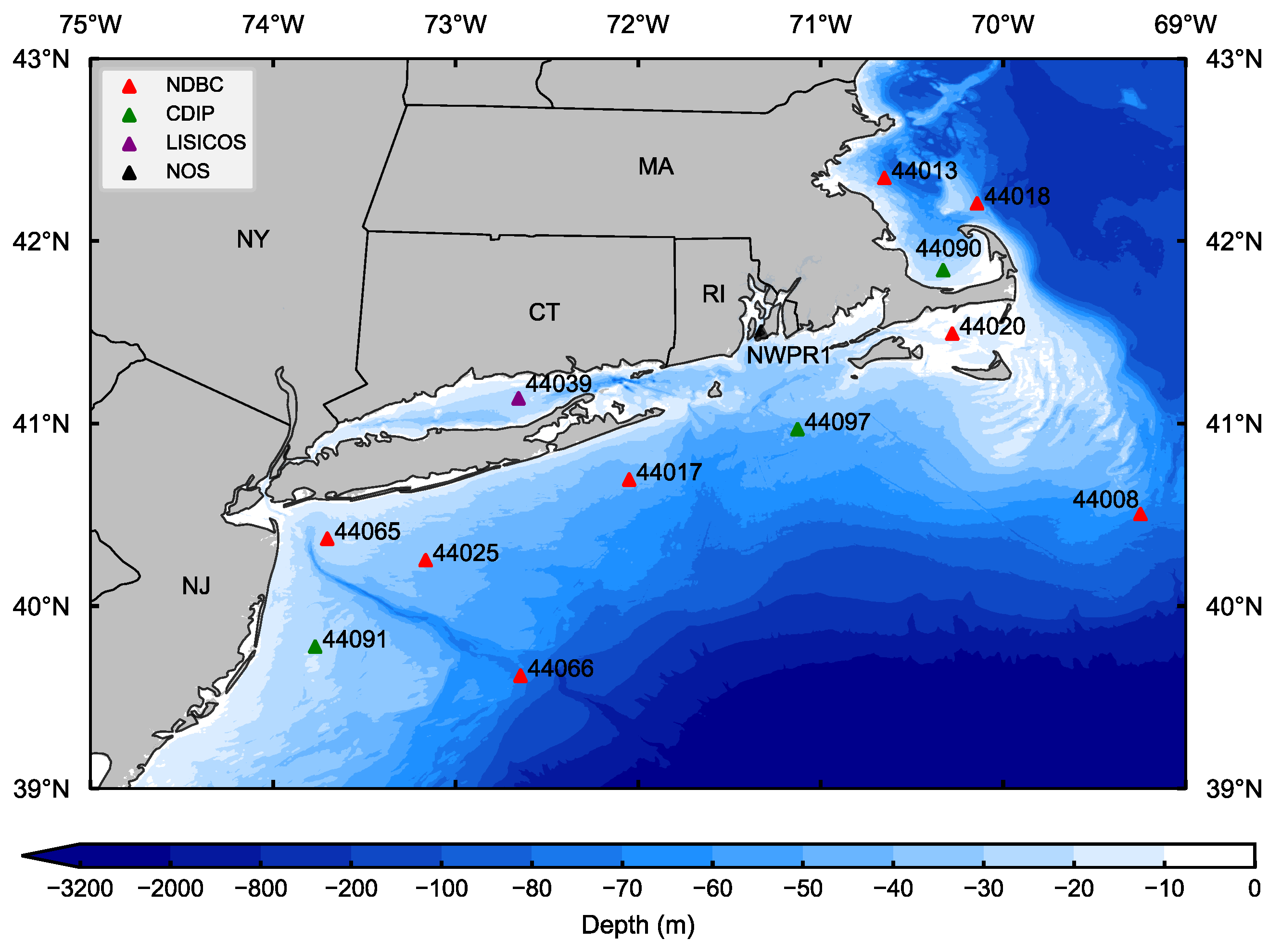
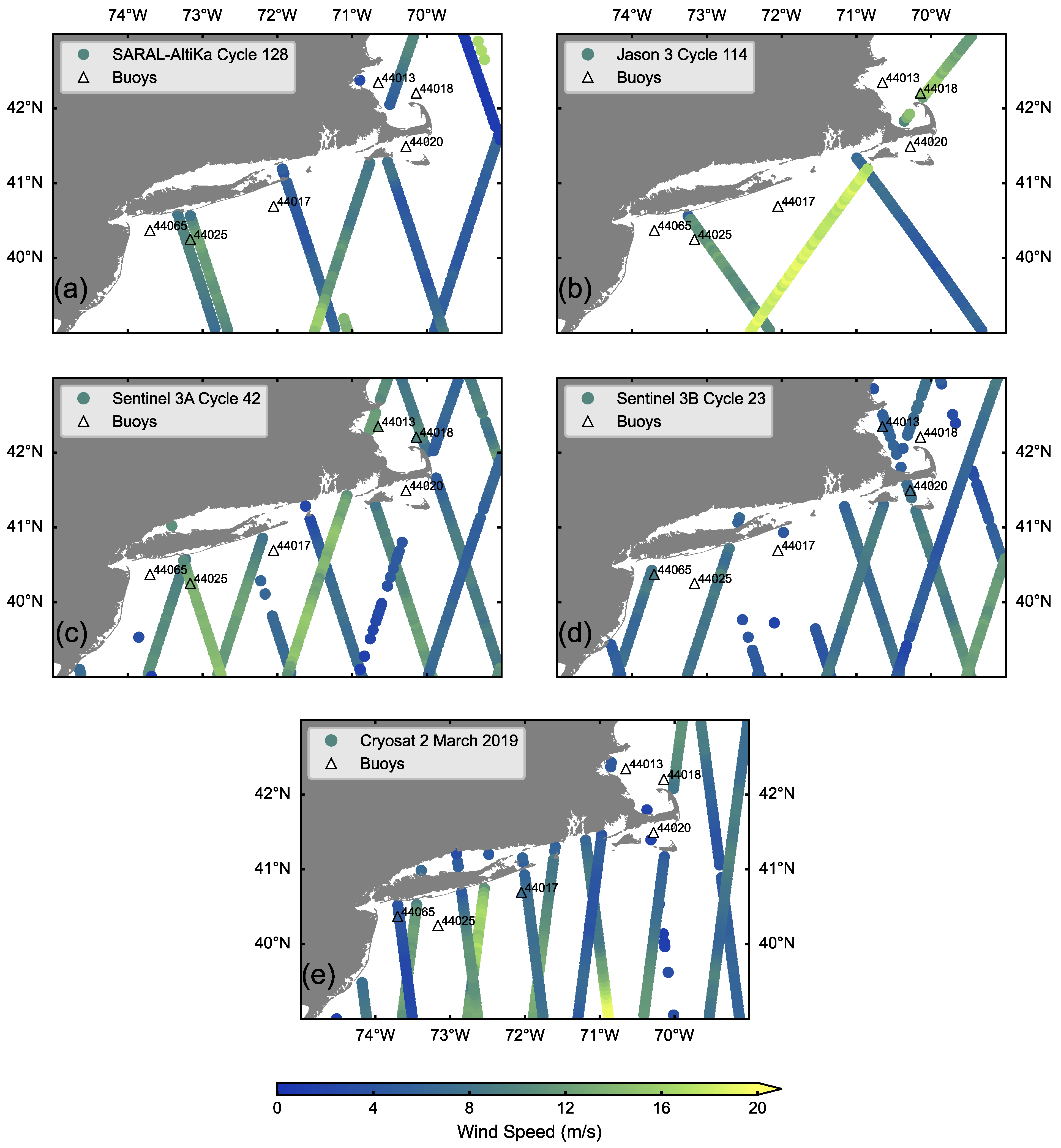
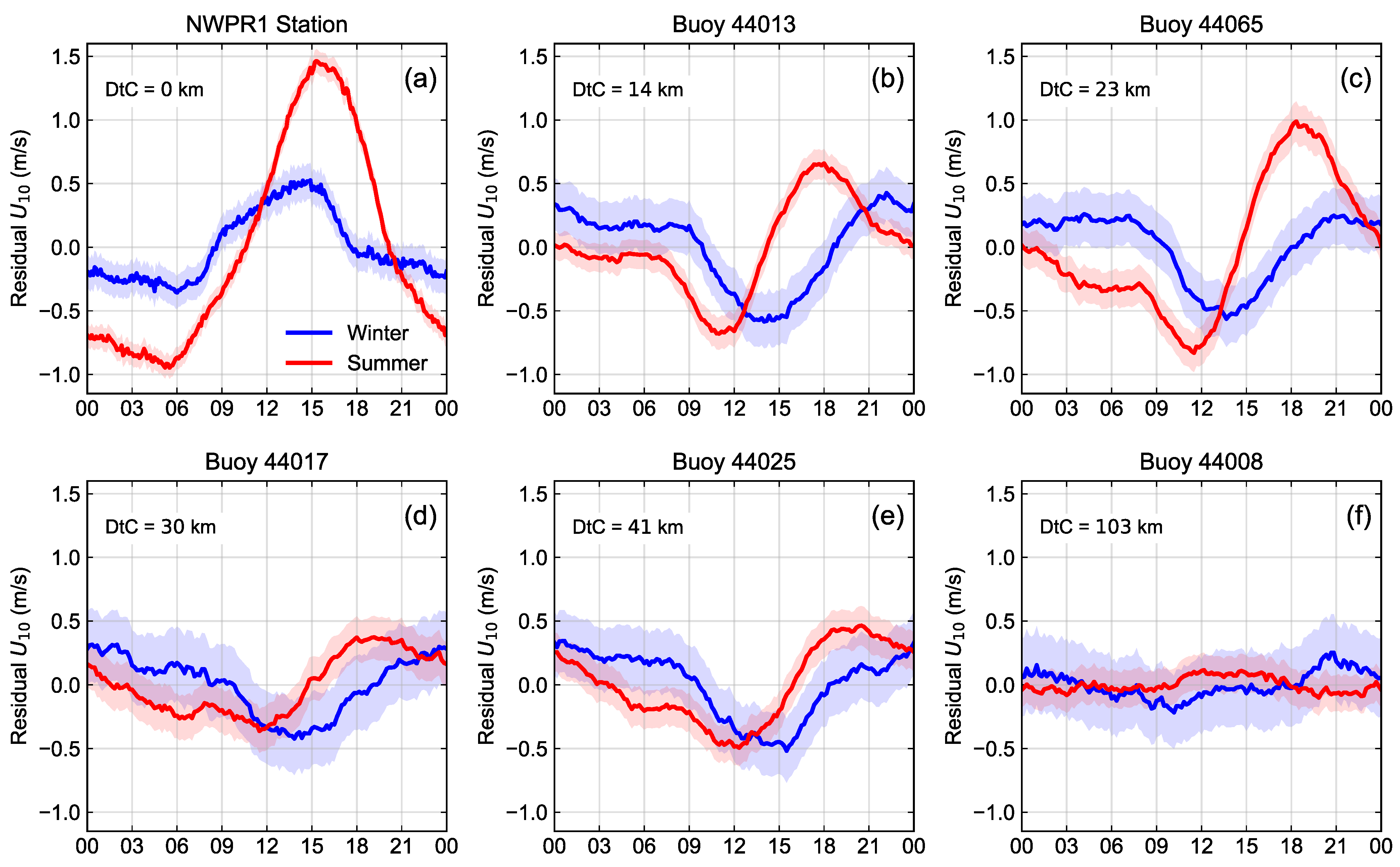
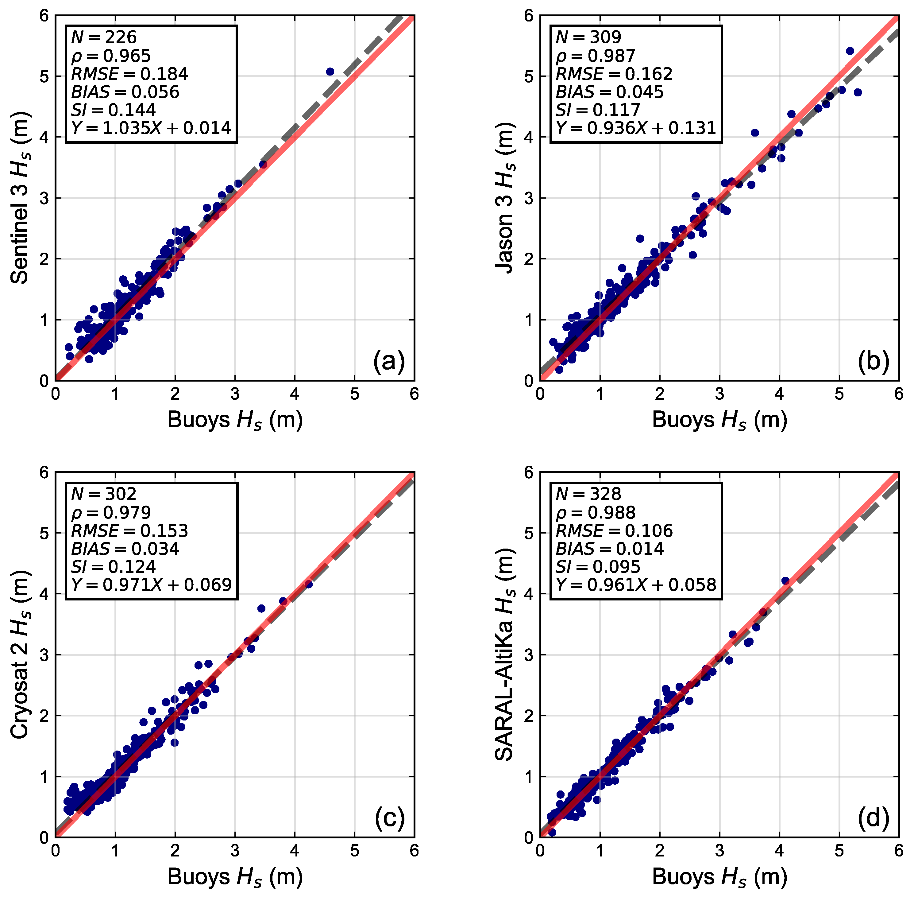
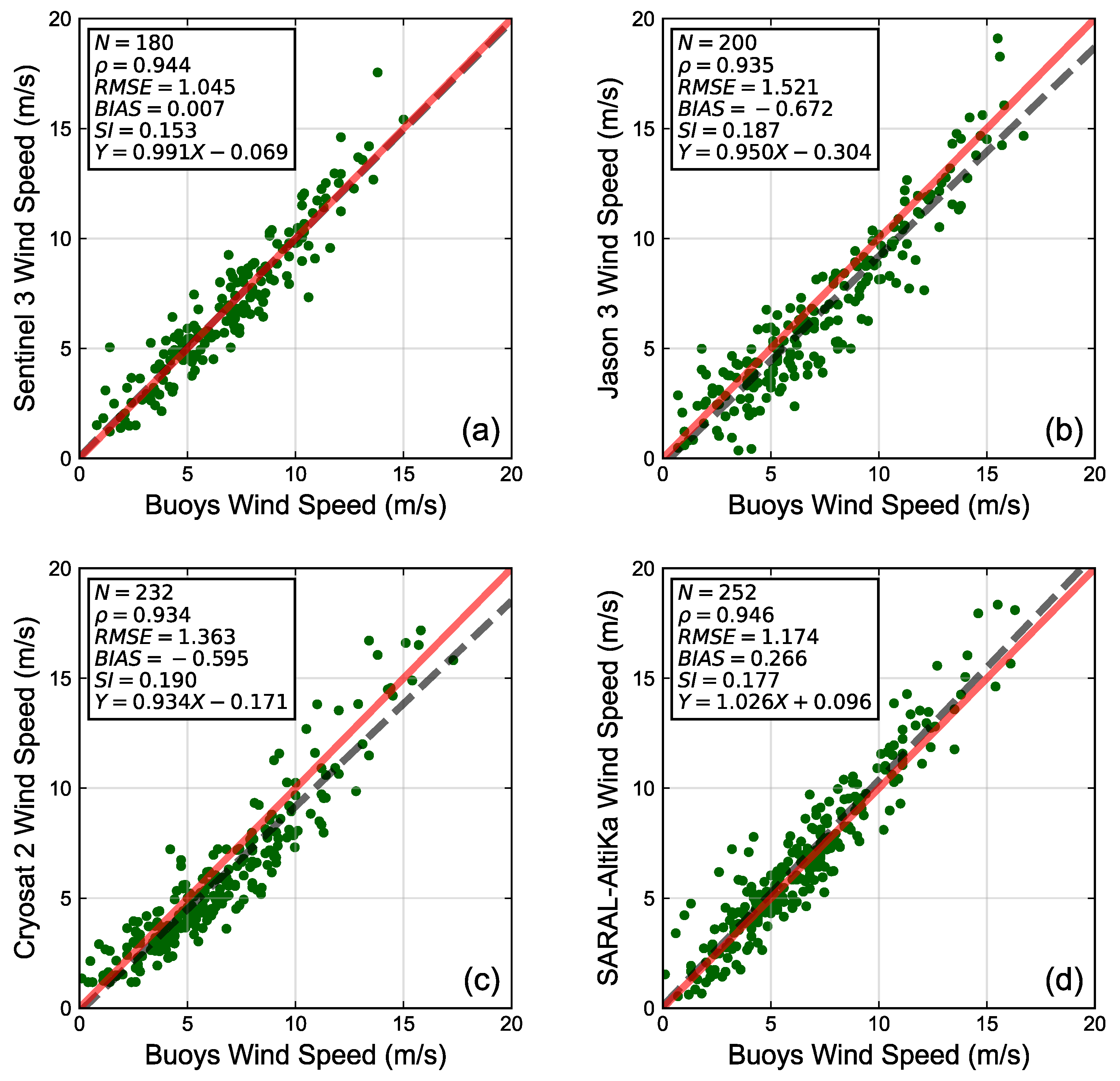
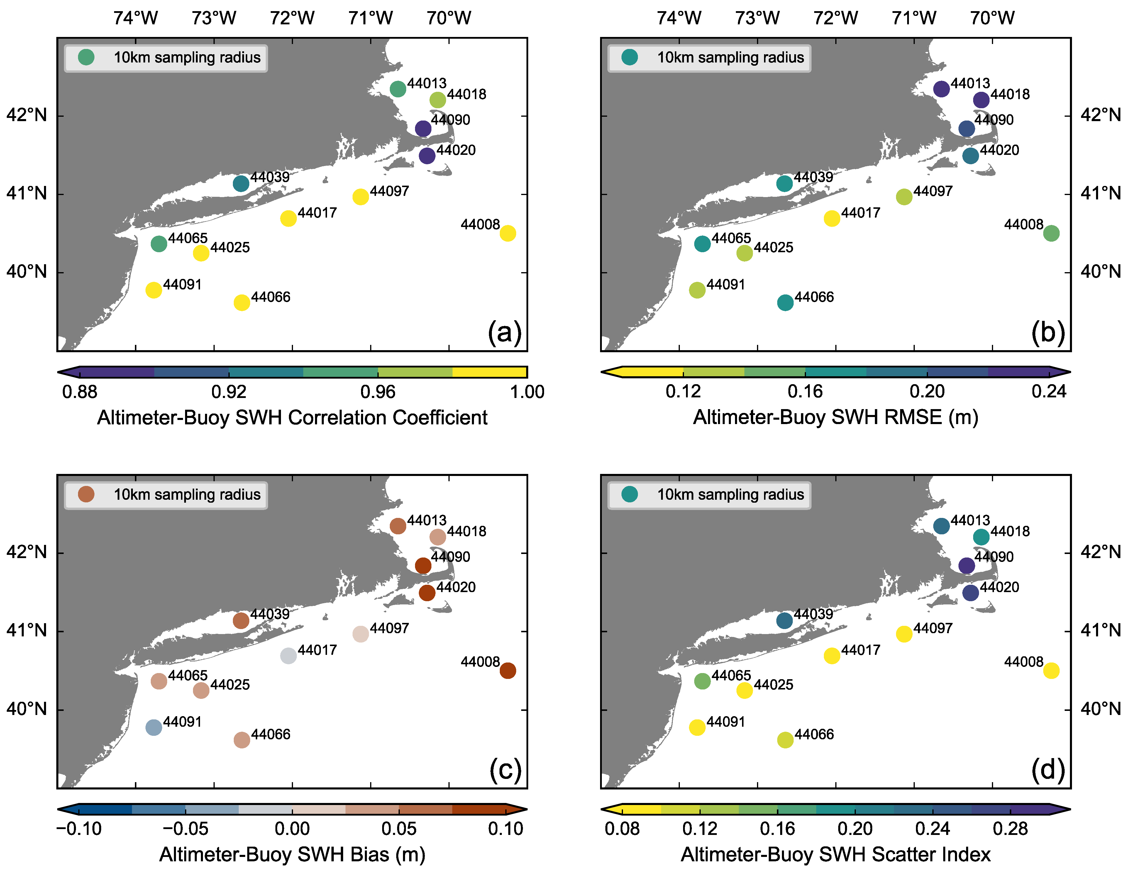
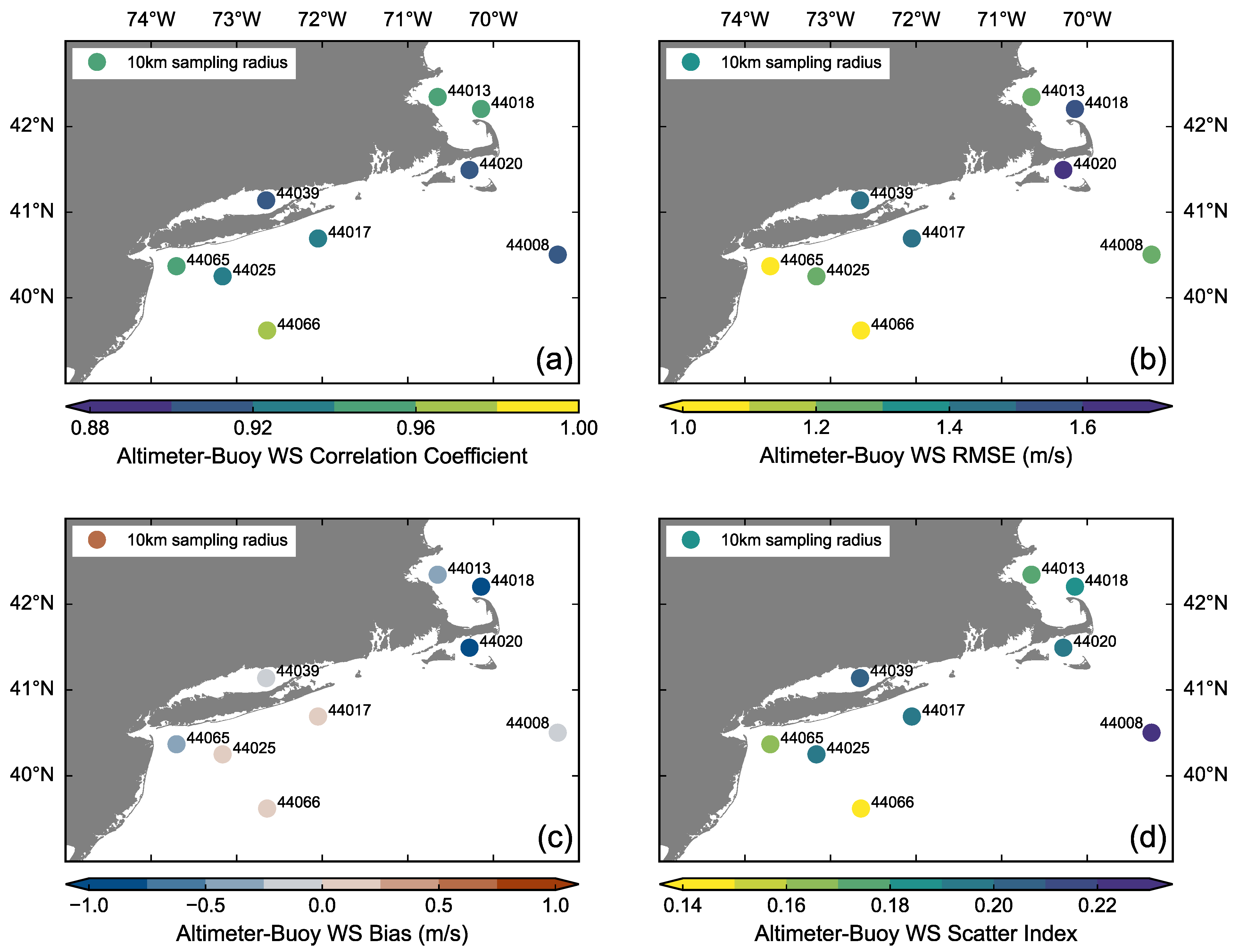
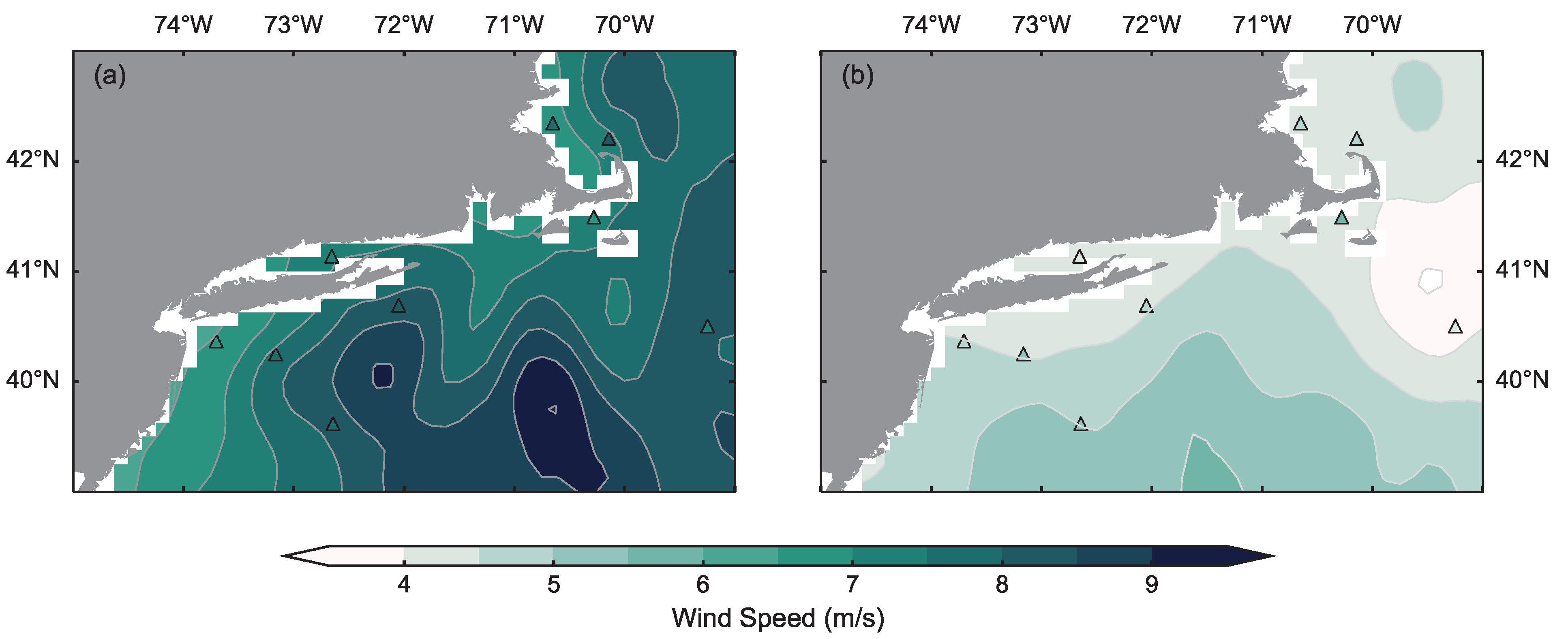
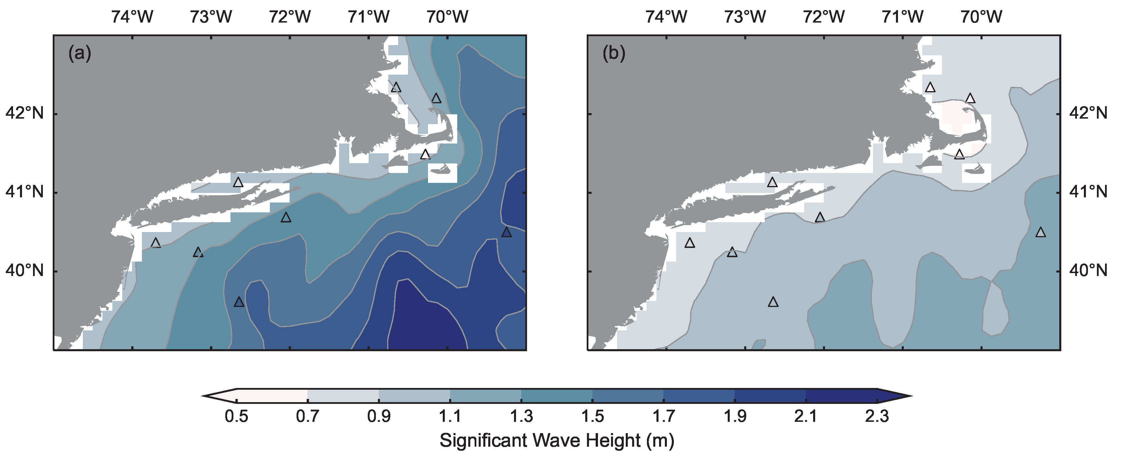
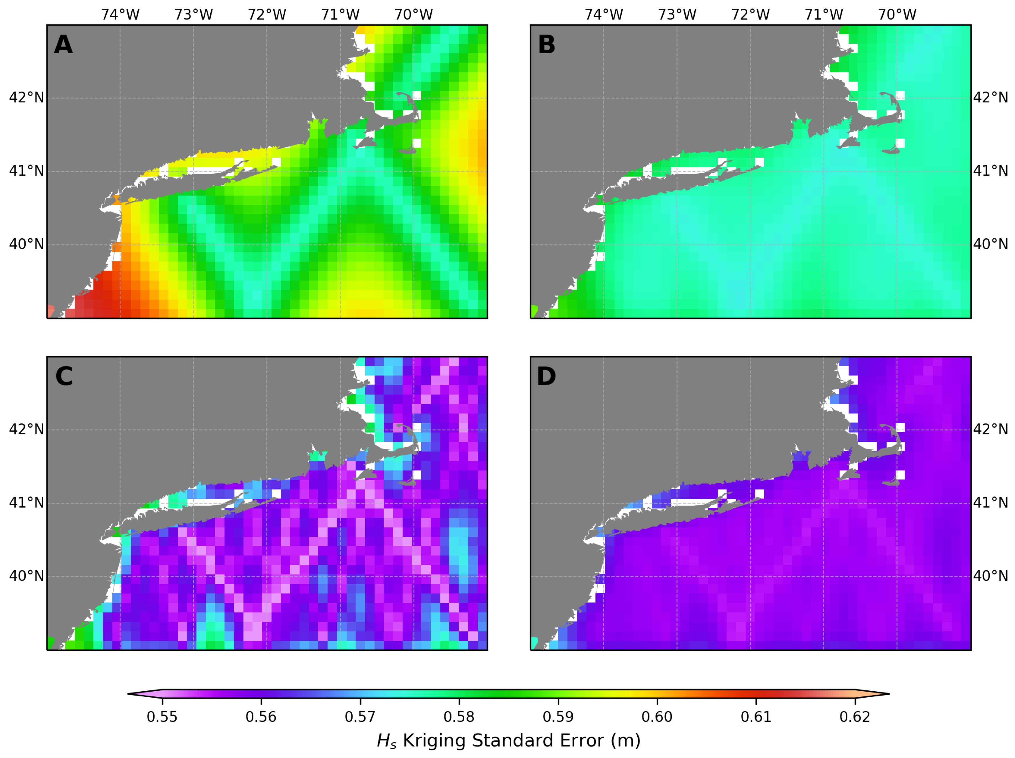
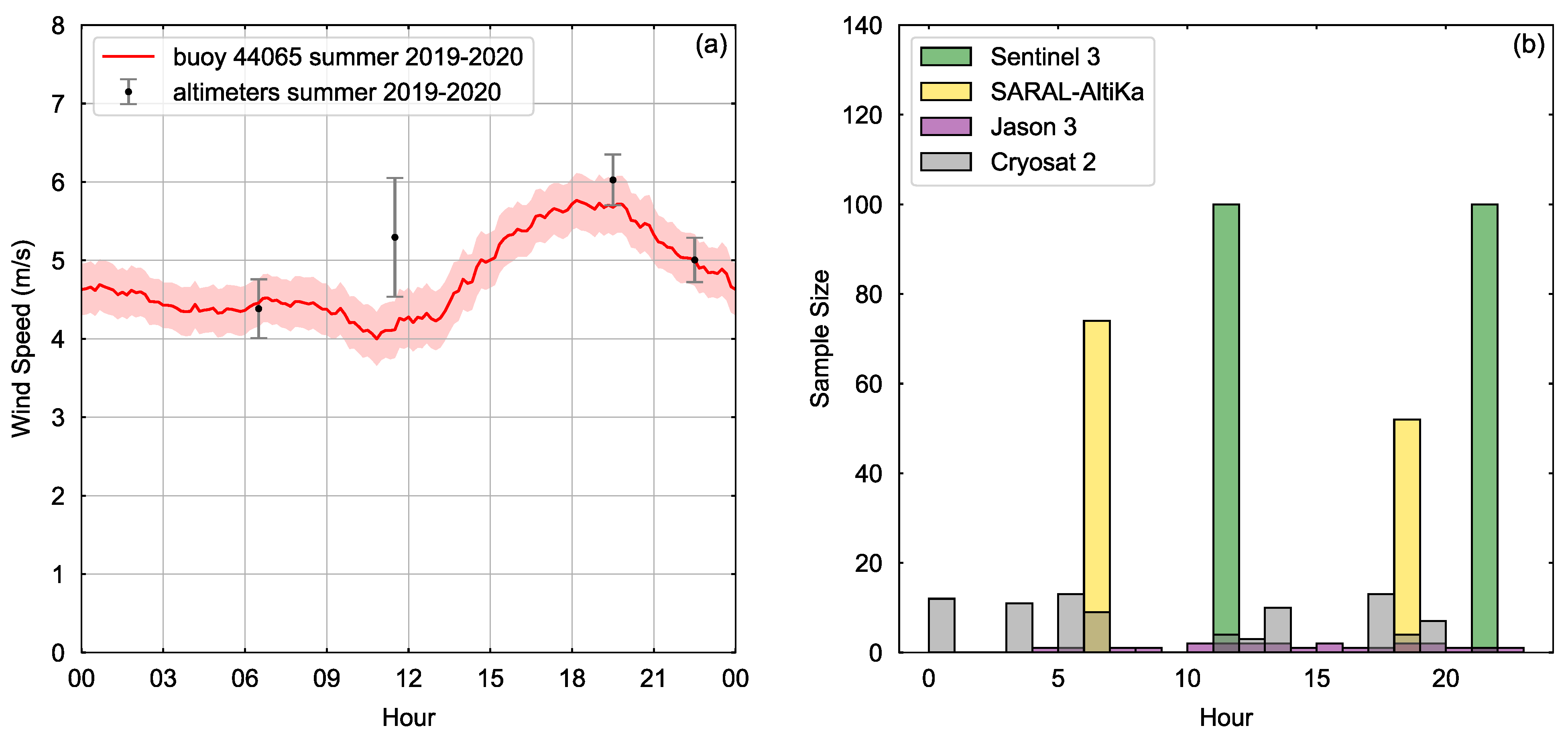
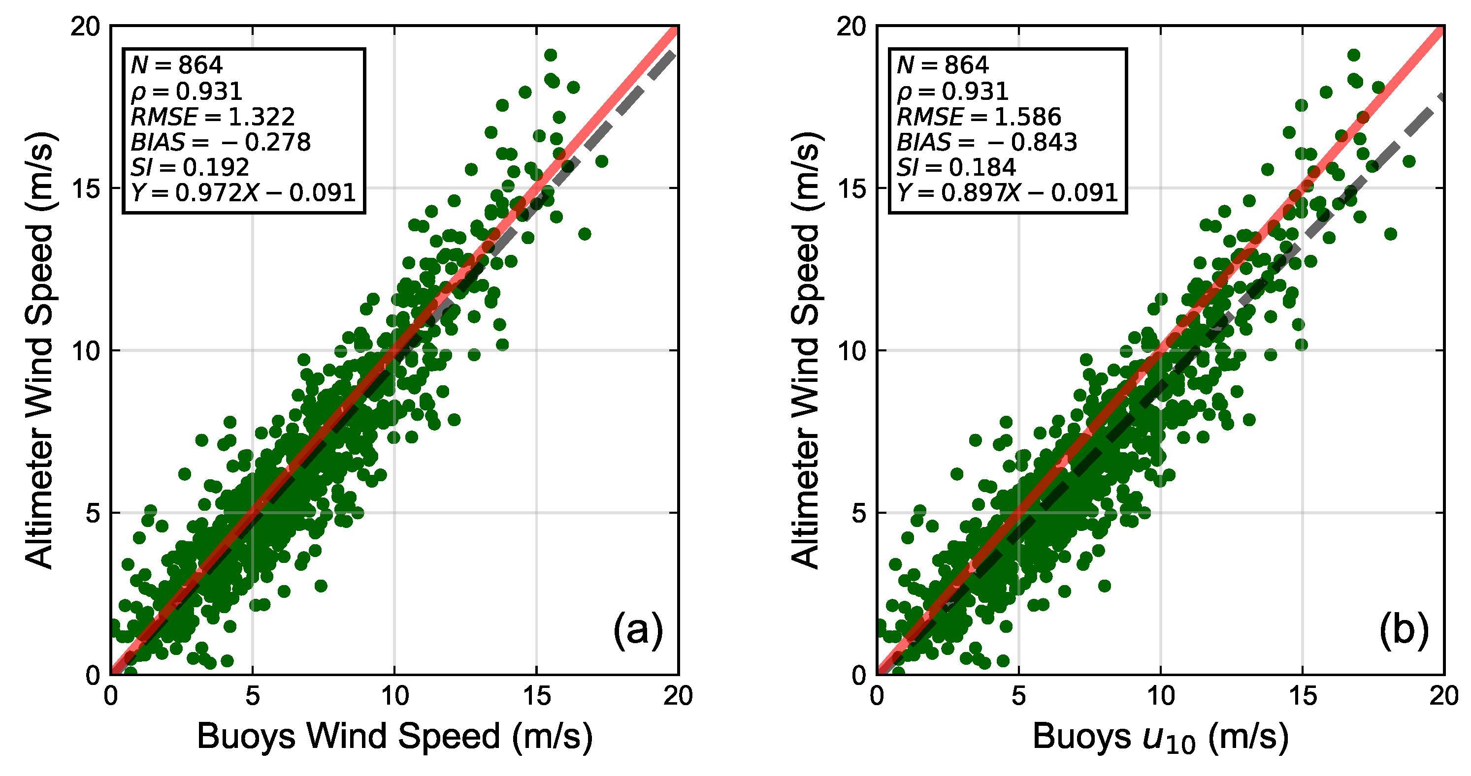
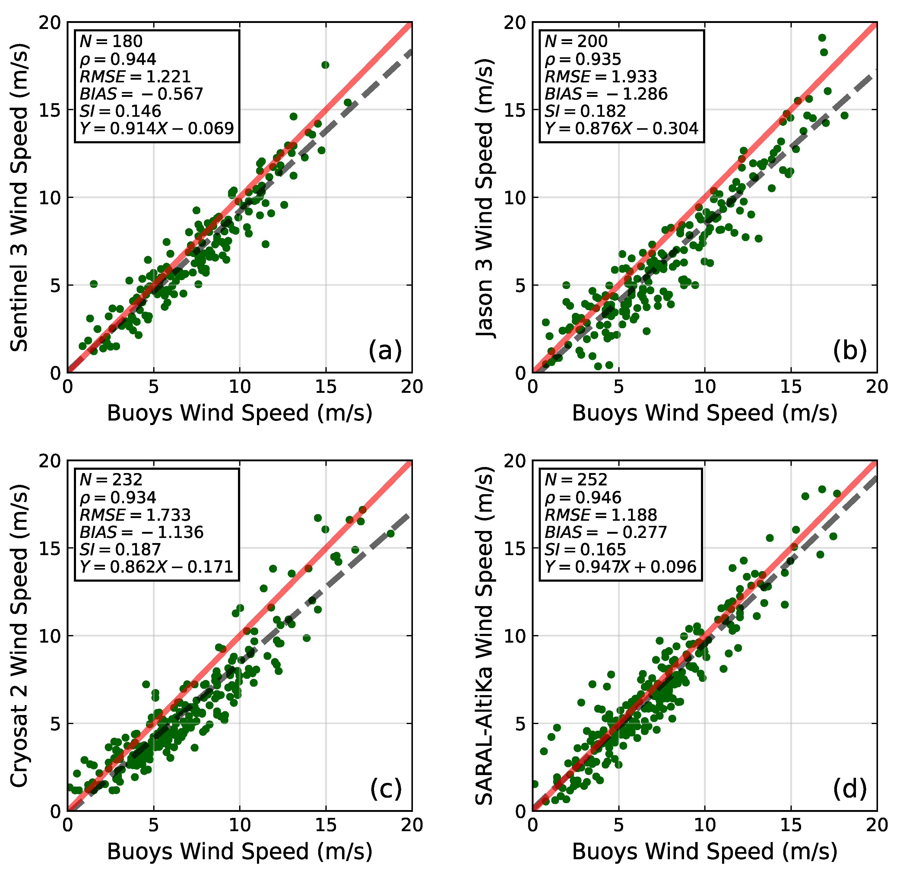
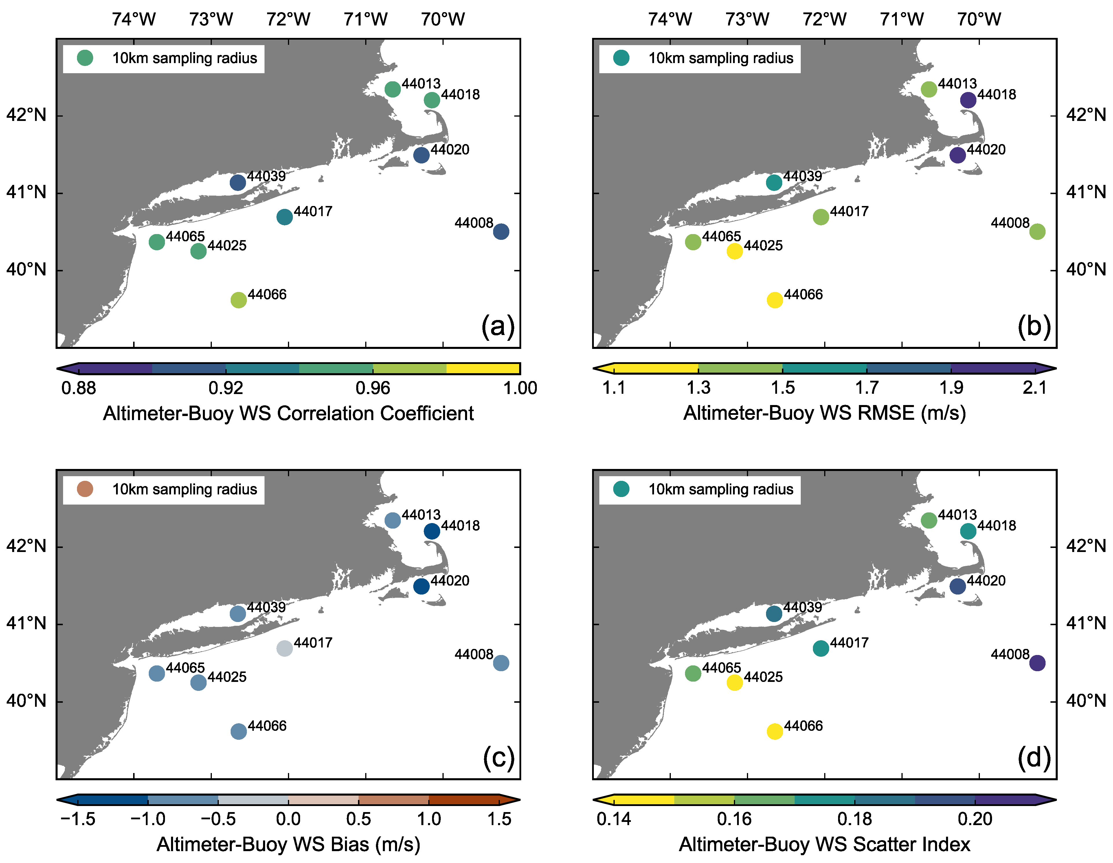
Table 1.
Satellite altimeters used in this study and their characteristics.
| SARAL | Jason 3 | Sentinel 3A | Sentinel 3B | Cryosat 2 | |
|---|---|---|---|---|---|
| Repeat Cycle | 35 | 10 | 27 | 27 | 369 |
| Frequency Band | Ka/C | Ku/C | Ku/C | Ku/C | Ku/C |
| Data Availability | 03/2013- | 09/2016- | 03/2016- | 05/2018- | 07/2010- |
| Instrument | AltiKa | Poseidon-3B | SRAL | SRAL | SIRAL |
| Operation Mode | LRM | LRM | SAR | SAR | LRM/SAR |
| Product Type | GDR | GDR | NTC | NTC | GOP |
Table 2.
The location, coordinates, anemometer height, water depth, and distance to the coast of the buoys used in this study.
Table 2.
The location, coordinates, anemometer height, water depth, and distance to the coast of the buoys used in this study.
| Buoy # | Location | Lon. (deg. W) | Lat. (deg. N) | Anem. Height (m) | Water Depth (m) | Dist. to Coast (km) |
|---|---|---|---|---|---|---|
| 44097 | Block Island, RI | 71.127 | 40.969 | - | 48.16 | 41 |
| 44020 | Nantucket Sound | 70.279 | 41.493 | 4.1 | 14.30 | 13 |
| 44025 | Long Island | 73.164 | 40.251 | 4.1 | 36.30 | 42 |
| 44017 | Montauk Point | 72.049 | 40.693 | 4.1 | 48.00 | 30 |
| 44065 | New York Harbor Entrance | 73.703 | 40.369 | 4.1 | 25.00 | 23 |
| 44039 | Central Long Island Sound | 72.655 | 41.138 | 3.5 | 27.00 | 13 |
| 44008 | Southeast of Nantucket | 69.248 | 40.504 | 4.1 | 74.70 | 103 |
| 44066 | East of Long Beach, NJ | 72.644 | 39.618 | 4.1 | 78.00 | 121 |
| 44091 | Barnegat, NJ | 73.769 | 39.778 | - | 25.60 | 27.5 |
| 44013 | Boston | 70.651 | 42.346 | 3.2 | 64.6 | 14 |
| 44090 | Cape Cod Bay | 70.329 | 41.84 | - | 25.9 | 11 |
| 44018 | Cape Cod | 70.143 | 42.206 | 4.1 | 41.5 | 13.5 |
Disclaimer/Publisher’s Note: The statements, opinions and data contained in all publications are solely those of the individual author(s) and contributor(s) and not of MDPI and/or the editor(s). MDPI and/or the editor(s) disclaim responsibility for any injury to people or property resulting from any ideas, methods, instructions or products referred to in the content. |
© 2023 by the authors. Licensee MDPI, Basel, Switzerland. This article is an open access article distributed under the terms and conditions of the Creative Commons Attribution (CC BY) license (https://creativecommons.org/licenses/by/4.0/).
Share and Cite
MDPI and ACS Style
Mitsopoulos, P.; Peña, M. Characterizing Coastal Wind Speed and Significant Wave Height Using Satellite Altimetry and Buoy Data. Remote Sens. 2023, 15, 987. https://doi.org/10.3390/rs15040987
AMA Style
Mitsopoulos P, Peña M. Characterizing Coastal Wind Speed and Significant Wave Height Using Satellite Altimetry and Buoy Data. Remote Sensing. 2023; 15(4):987. https://doi.org/10.3390/rs15040987
Chicago/Turabian StyleMitsopoulos, Panagiotis, and Malaquias Peña. 2023. "Characterizing Coastal Wind Speed and Significant Wave Height Using Satellite Altimetry and Buoy Data" Remote Sensing 15, no. 4: 987. https://doi.org/10.3390/rs15040987
Note that from the first issue of 2016, this journal uses article numbers instead of page numbers. See further details here.