

Numerical Study on the Effects of Intraseasonal Oscillations for a Persistent Drought and Hot Event in South China Summer 2022

1
Key Laboratory of Meteorological Disaster, Ministry of Education, School of Atmospheric Sciences, Nanjing University of Information Science & Technology, Nanjing 210044, China
2
Chongqing Climate Center, Chongqing 401147, China
*
Author to whom correspondence should be addressed.
Remote Sens. 2023, 15(4), 892; https://doi.org/10.3390/rs15040892
Submission received: 16 December 2022
/
Revised: 24 January 2023
/
Accepted: 3 February 2023
/
Published: 6 February 2023
(This article belongs to the Special Issue Understanding the Meteorological Environment in Arid Regions through the Integrative Analyses of Remote Sensing, Ground Observational Stations and Numerical Models)
Abstract
:From 19 July 2022 to 31 August 2022, a rare persistent drought and heat event occurred in the middle of the Yangtze River basin (MYRB). Normalized difference vegetation Index (NDVI) over 25% of the area decreased more than 0.05 compared with the climatology, causing extremely agricultural drought disaster and economic losses to China. Previous studies have shown that the occurrence of compound drought and heat events (CDHEs) in the MYRB was associated with intra-seasonal oscillations (ISOs) from different latitudes. Nevertheless, what was the role of ISOs at different latitudes in the formation of the CDHE? To address this question, this paper designed a numerical simulation experiment of partial lateral forcing to investigate the changes in meteorological elements by removing the signals of ISOs on different lateral boundaries. We found that the wave series formed in the upper troposphere at 200 hPa played a significant role in the occurrence of the CDHE in the northern part of the MYRB in this progress. It was found that the ISO component of the northern boundary caused the mean temperature to rise by 2.4 °C and aggravated the drought in 53.7% of the region. On the other hand, the anticyclone anomaly in the lower troposphere at 800 hPa had a continuous impact on the southern and eastern boundaries. It was found that the ISO component of these two boundaries can increase the average temperature by 1.93 °C in the MYRB and intensify the drought in 49.7% of the area. In the developing period of the CDHE, the South Asian high and the Western North Pacific subtropical high were coupled with each other and jointly controlled the MYRB, so that the significant positive geopotential height anomaly stayed above the MYRB for a long time, which was conducive to the development of local subsidence. The results of this paper will help to better understand the formation mechanism of CDHEs in the MYRB and assist meteorologists to prevent and forecast the occurrence of CDHEs in advance.
1. Introduction
The latest study from the Intergovernmental Panel on Climate Change (IPCC) shows that the average surface temperature of Earth has risen at a rate faster than any prior 50-year period in the preceding two thousand years [1]. Although China has made great contributions to controlling the greenhouse effect, the warming rate of China is apparently higher than that of other countries during the same period. Using temperature data from 360 stations throughout China spanning 50 years, Zhang et al. [2] discovered a yearly increase in surface soil temperature of 0.0038 °C. Simultaneously, several regions in China have seen an alarming upward trend in the regularity, severity, and total area impacted by intense heatwave occurrences. Moreover, the growing frequency of compound drought and heat events (CDHEs) has led to substantial losses in the agricultural and manufacturing sectors [3]. Among them, the possibility is frequent that CDHEs occur in the middle of the Yangtze River basin (MYRB) and eastern China [4,5]. Farmers cannot gather crops, and workers are unable to create wealth, because of CDHEs. Therefore, it is incumbent upon those working in meteorology to investigate the causes of CDHEs and provide accurate forecasts.
It was reported that the greenhouse effect and atmospheric circulation anomalies brought about regional heatwave events. Regional CDHEs are often induced by atmospheric circulation anomalies, such as those brought on by the El Nino-Southern Oscillation (ENSO) [6,7,8]. One of the key drivers of regional CDHEs in the MYRB is a large-scale atmospheric anomaly caused by the eastward and northward anomalies of the South Asian high (SAH) and the northward anomaly of the subtropical high ridge [9]. The sub-seasonal atmospheric system is the culprit behind the continuous circulation anomaly. The heatwave events and precipitation anomalies that are located in southern China and the MYRB are connected to intraseasonal oscillations (ISOs) [10,11].
Sub-seasonal fluctuations from tropical areas and low-frequency fluctuations from mid-high latitudes usually occur in the MYRB [12]. Consequently, both types of fluctuations further influence the CDHEs over the MYRB [13,14]. For instance, Hsu et al. [15] found that ISOs originating from mid-to-high latitudes had a significant impact on the frequency with which heatwave events occur across the MYRB. Lu et al. [16] discovered that the warm and moist air carried by the tropical atmospheric convection and the cold air activity accompanied by the propagation of the Rossby wave train in the mid-high latitudes induce water vapor convergence in the southern region of China. They also demonstrated that the tropical and mid–high latitudes are impacted by atmospheric ISO signals, which has implications for the sort of aberrant precipitation events occurring in the southern hemisphere.
Sub-seasonal atmospheric oscillations from different latitudes interact, creating a central topic in the study of persistent CDHEs in the MYRB. However, how to differentiate between ISOs from various latitudes in terms of their contributions to CDHEs is still an unanswered question. The regional climate model, which employs dynamical downscaling techniques to take local topography information into account, is more successful than the global climate model for studying sub-seasonal climatic systems [17]. By comparing the outcomes of numerical simulations with ISO signals over a certain time period, some meteorological researchers attempt to quantify the impacts of various signals on regional climatic anomalies. For example, Hu et al. [18] studied the characteristics and causes of the dominant ISO that controlled the eastern Tibetan Plateau summer rainfall (ETPSR), and they discovered that the ISO over the ETPSR exhibits a vertical dipole pattern of geopotential height during the dry phase. Shi et al. [19] found a significant influence of BSISO on tropical cyclone (TC) rainstorms along the southeast coast of China by diagnosing the link between BSISO in eight different phases and monsoon rainstorms.
From late July to August 2022, a large-scale continuous CDHE occurred in the MYRB. The high-temperature weather in August was the most serious in the same period of history in China since 1961. It had characteristics of a long duration, a wide range of influence, and obvious extremeness. Affected by the high temperature, the area of affected crops in some provinces reached 4.076 hectares, including Sichuan, Hunan, Hubei, etc. [20]. Furthermore, the CDHE also caused a large quantity of wildfires in this period, which resulted in direct economic losses of CNY 32.8 billion. For the purposes of this paper, “PLF” refers to the partial lateral forcing experiment developed for WRF by Yang and Wang [21]. The experiment combines numerical simulation methods and dynamic diagnostic analysis to explore the development mechanism of the above CDHE.
2. Materials and Methods
2.1. Dataset and Methods
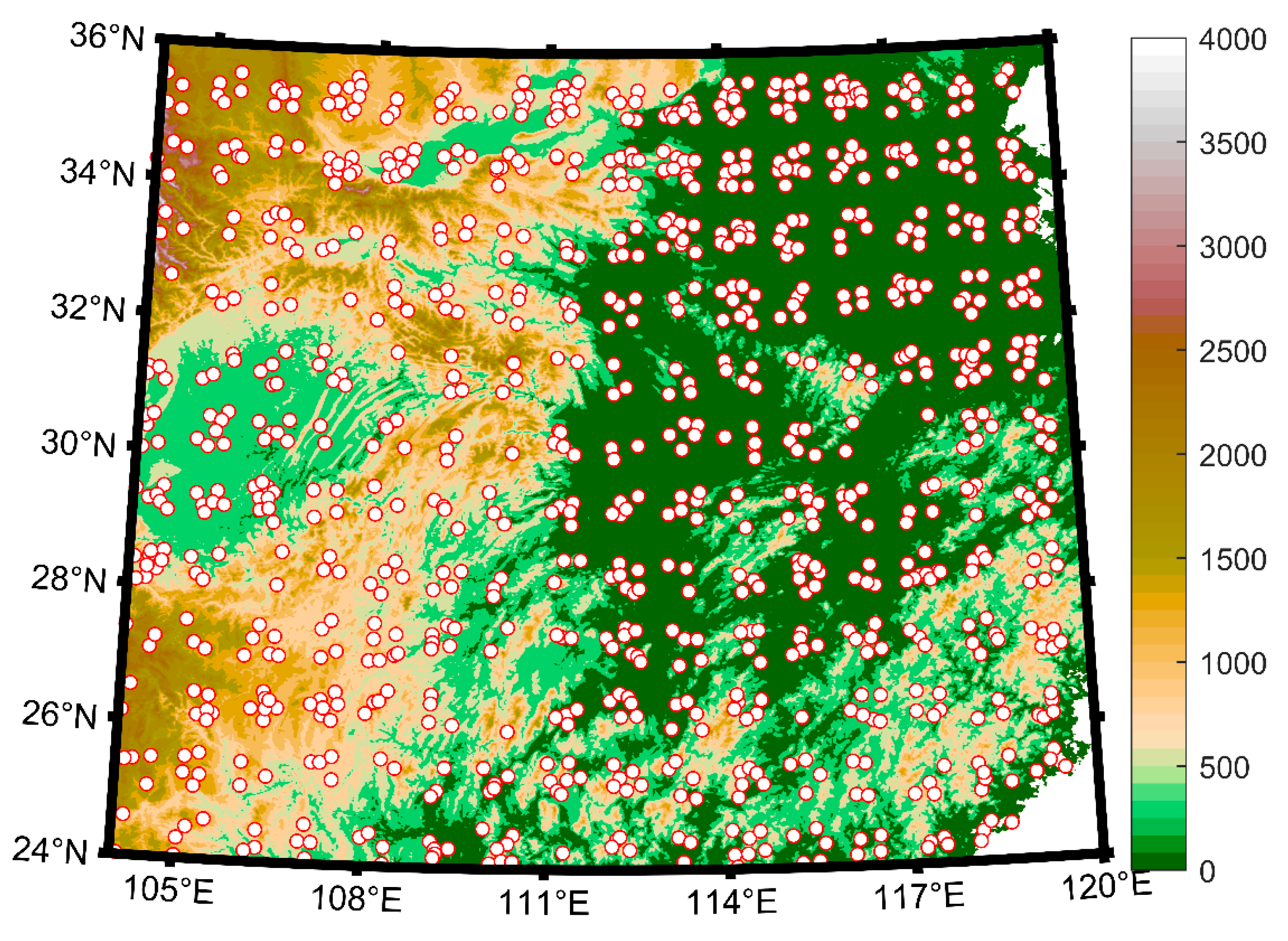
In this research, concentration was primarily on the MYRB in South China (24°–36°N, 104°–120°E). The dataset included the ERA5 reanalysis data provided by the European Centre for Medium-Range Weather Forecasts, with grids of 0.25° × 0.25°, consisting of 37 layers in the vertical direction and 4 layers of ground soil data [22]. For assessing vegetation status, the versatility of normalized difference vegetation index (NDVI) has surpassed all other indices, as noted by Huang et al. This is because of its easy accessibility, long history, and simplicity [23]. In addition, we chose to use the NDVI datasets from the National Aeronautics and Space Administration that cover the years 2000 to the present. The grid was 0.05° × 0.05° and included 13 layers of scientific datasets [24]. The satellite NDVI is derived from the MODIS/Terra Vegetation Indices 16-day L3 Global 0.05Deg CMG V006 dataset [25], and is used to monitoring drought conditions. We focus on the studying period of this CDHE. Therefore, two 16-day periods (28 July–12 August and 13 August–28 August) were used, and the horizontal resolution was 0.05° × 0.05°.
As a CDHE contains two parts, the heatwave event and the drought event, the criteria of the two events need to be given separately when defining such compound disasters. These two criteria are explained below. According to the criteria established by Qi et al. [26], a heatwave event across the south China may be recognized if the daily mean temperature in a region rises beyond the 95th percentile for at least two consecutive days (defined over 1981–2010). A drought event can be recognized when more than 50% of the stations have a meteorological drought composite index (MCI) less than −1. Xie et al. discovered that the MCI index was superior to the standardized precipitation index, the standardized weighted precipitation index, and the moisture index in terms of geographical and temporal drought diagnostic capacity, diagnostic ability for typical drought processes, and correlation with drought disaster over the MYRB [27]. The MCI information used station data provided by the National Climate Center of China, and 943 stations in the MYRB were chosen to analyze their respective data (Figure 1).
The MCI corresponding to different drought levels is shown in Table 1.
The above table shows that at least 50% of the stations reached the level of moderate drought at the time of drought events. In this study, the MCI is calculated with reference to the Grades of Meteorological Drought 2017 edition [28], and the formula is shown as follows:
where is the seasonal adjustment coefficient and = 1.2 for South China in July/August. , , , and are weighting factors and = 0.5, = 0.6, = 0.2, and = 0.1 for this research. Additionally, and represent the standardized precipitation index for the previous 90 and 150 days, respectively. is the standardized weighted precipitation index for the previous 60 days and represents the moisture index for the previous 30 days, with the intermediate variable PET (potential evapotranspiration) calculated with the Thornthwaite method [29]. To assess the accuracy of each run’s drought simulation, the MCI index was computed day-by-day at each grid point using the aforementioned definition. In summary, the two criteria above were combined and CDHE was defined as follows. A CDHE is considered to have occurred if both high temperature events and drought events occur within seven consecutive days. The start and end of CDHE are determined by both the high temperature event and the drought event.
The above definition shows that the occurrence of CDHEs at small and medium scales is closely relevant to the local temperature tendency, and the probability of CDHEs occurring increases when the local temperature is high. Horizontal temperature advection, adiabatic processes generated by vertical motion, and the apparent heat source in the atmosphere all play a role in shaping the local temperature trend, which may be formulated as [30]:
where represents static stability, with R representing the gas constant and representing the specific heat at constant pressure, and represents the diabatic heating, which includes radiative heating, latent heating, surface heat flux, and subgrid-scale processes. The four terms in Equation (2) stand for the temperature tendency, horizontal advection of temperature, vertical transport, and diabatic heating. Using ERA5 meteorological data, we estimated the temperature balance at 800 hPa across time intervals to isolate the effects of these four distinct physical processes. Meteorological data from ERA5 were used to determine the first three terms, and the fourth term was derived from the first three [31].
Furthermore, the ISO component was extracted by first subtracting the summer mean from the ERA5 meteorological reanalysis data and then subtracting the synoptic fluctuations by using a 5-day running mean to locate regions of significant anomalies in the ISOs, all in reference to the method by Lu et al. [32]. There is also a need to determine the moving propagation direction of the ISOs as the basis for numerical experiments. The wave action fluxes commonly used in the current atmospheric dynamic diagnosis of Rossby wave propagation are the Plumb wave action flux, the TN wave action flux, and the local EP flux, respectively. Shi et al. [33] demonstrated that the TN wave action flux was an improvement on the Plumb wave action flux, and had the advantage of directly reflecting the time-to-time evolution of Rossby long waves compared with the local EP flux. In brief, we adopted the TN wave action flux, which is more suitable for the diagnostic requirements of this study, and the formulation is expressed as [34]:
where is the transverse momentum flux of TN waves, is the wind speed, and and are the zonal and meridional winds, respectively. Partial derivatives are denoted by subscripts, and the parameter stands for the stream function.
2.2. Model and Experimental Design
The Weather Research and Forecasting Model (WRF V4.4), a regional and nonhydrostatic atmospheric simulation system using sigma terrain tracking coordinates [35], was used for this study. All trials were conducted between 19 July and 31 August. According to previous studies on simulations of drought events in South China, our chosen parameterization schemes included the WSM3 cloud microphysics scheme [36], the CAM longwave and shortwave radiation schemes [37], the MYJ near-surface and boundary layer schemes [38], the Noah land surface model [39], and the Betts–Miller–Janjic cumulus scheme [40,41].
The simulation area roughly covers the region of 24–36°N, 104–120°E, with a horizontal grid distance of 9 km and a boundary buffer set at 5 grid points. The initial field, as well as the boundary conditions for the experiment, were taken from the ERA5 reanalysis data at 6-h intervals, with a total of 37 layers to 1 hPa in the vertical direction aloft, including horizontal wind, geopotential height, vertical velocity, and specific humidity. The soil data included 4 layers down to 289 cm below the surface, including soil temperature and moisture.
In this article, we aim to answer the following two questions. How much do different ISO signals in the tropics and mid- and high-latitudes contribute to this persistent CDHE? How can the contribution of the ISO signals be distinguished? To answer these two questions, we made use of the PLF experiments designed by Yang and Wang [21]. Yang et al. already conducted the PLF experiment in 2015 to examine an exceptional heavy rainfall event that happened in East Asia in 1998 [42], and again in 2018 they used it to analyze the TC05A [21], which occurred in November 2011. Both experiments yielded excellent outcomes, demonstrating that the PLF experiment is an effective tool for discovering the main components governing extreme events via regional climate modeling. Even though it has been used in several studies that show its benefits, the most important reason is that it can quantitatively analyze the influence of ISOs from different latitudes. Consequently, the selection of the PLF experiment was necessary and appropriate for our investigation. First, the boundary field with the ISO signal removed was defined as the boundary field for the sensitivity experiment, with the initial field unchanged. Second, based on the observation results, three sensitivity experiments, RMV-N, RMV-SE, and RMV-NSE, were carried out, representing the removal of the ISO signals at the northern boundary, the southern and eastern boundaries, and all three boundaries, respectively. Our research indicated that the upper troposphere affected the northern boundary of the MYRB, whereas the lower troposphere influenced the eastern and southern boundaries of the MYRB, as discussed in detail in Section 3.1, which led us to choose these three sensitivity experiments. In generating boundary fields for sensitivity experiments, the respective intraseasonal signals were removed for all meteorological elements on the corresponding sides, including wind speed, temperature, and specific humidity. The final conclusions were obtained by using a two-sample t-test to test the significance of the differences between the sensitivity and control experiments. The same physical parameterization scheme is used for each experiment. Details of the experiments are presented in Table 2.
3. Results and Discussion
3.1. Overview of the Event
From 19 July 2022 to 31 August 2022, a rare CDHE occurred in southern China whose influence range was the largest in the same period in history, causing extremely serious economic losses within China. It triggered widespread drought, low lake water levels, and reduced food production [43]. Therefore, mathematical and statistical methods were used and wavelet analysis was performed on the ISO component of the area average surface temperature () to further understand the cause of this event.
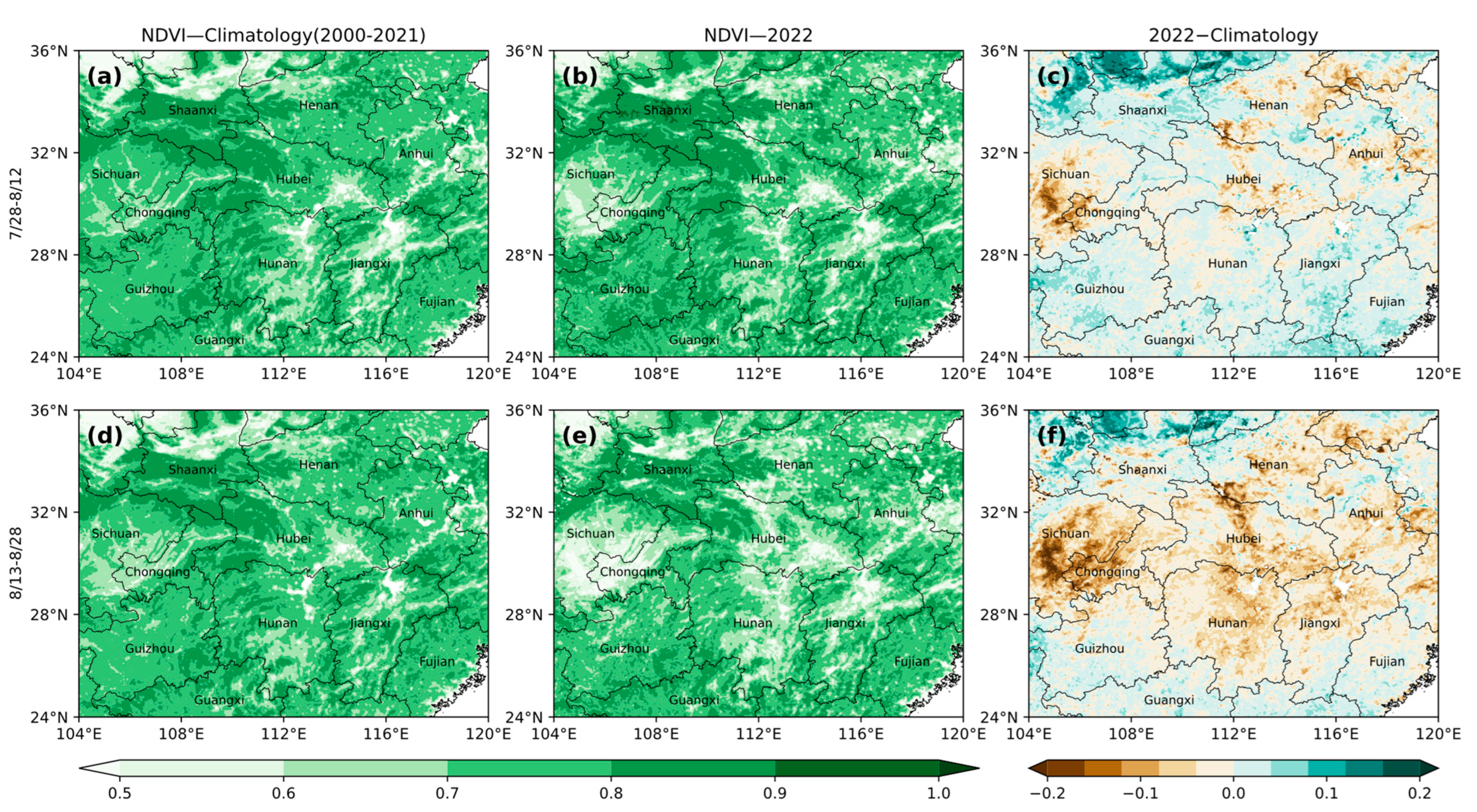
The NDVI in South China in early (28 July–12 August) and late (13 August–28 August) August is shown in Figure 2. By comparing the climatology NDVI with the 2022 index, it is clear that in late August the NDVI dropped in a large area in South China, and the NDVI in the MYRB over 25% areas deceased more than 0.05 compared with the climatology. Moreover, the decline in NDVI in eastern Sichuan and western Chongqing reached 0.2, leading to widespread wildfires in the mountain areas in Chongqing. There was also considerable decline in northern Hubei and southern Henan and the area with a declining NDVI corresponded with the drought area generally. In early August, there was also a small part of area in showing a decline trend but not that significant as in late August, indicating that the drought event mainly occurred in late August, in correspondence with the data shown in Figure 3.
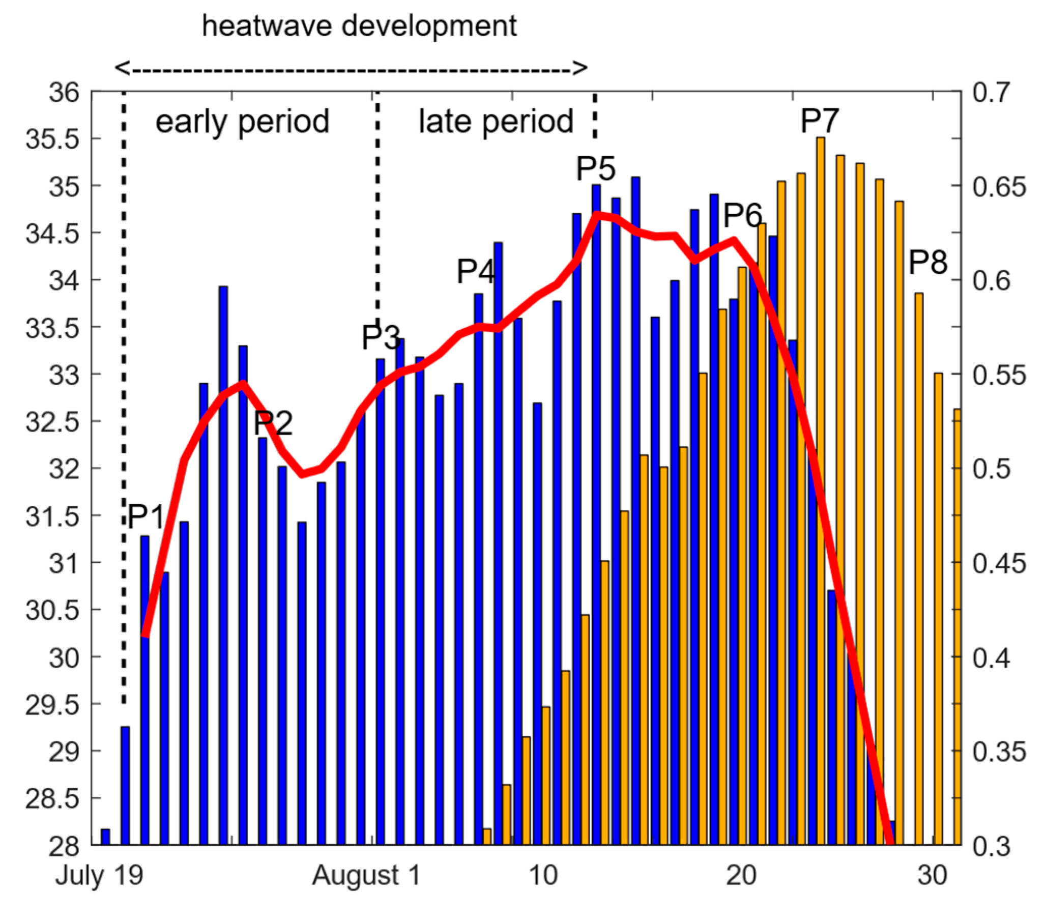
As shown in Figure 3, the area average maximum temperature from 24 July to 27 July and 1 August 1 to 25 August remained at 32 °C and above and reached a maximum value of 35 °C near 13 August. The temperature anomaly in the eastern plain area reached 2–3 °C relative to the same period in history, and the temperature anomaly in the western Sichuan-Chongqing area was as high as 5 °C. Due to the decrease in precipitation caused by this event, it can be seen from the MCI index that the proportion of stations having a moderate drought or more severe conditions increased rapidly after 7 August, jumping to a maximum of 67.5% on 24 August.
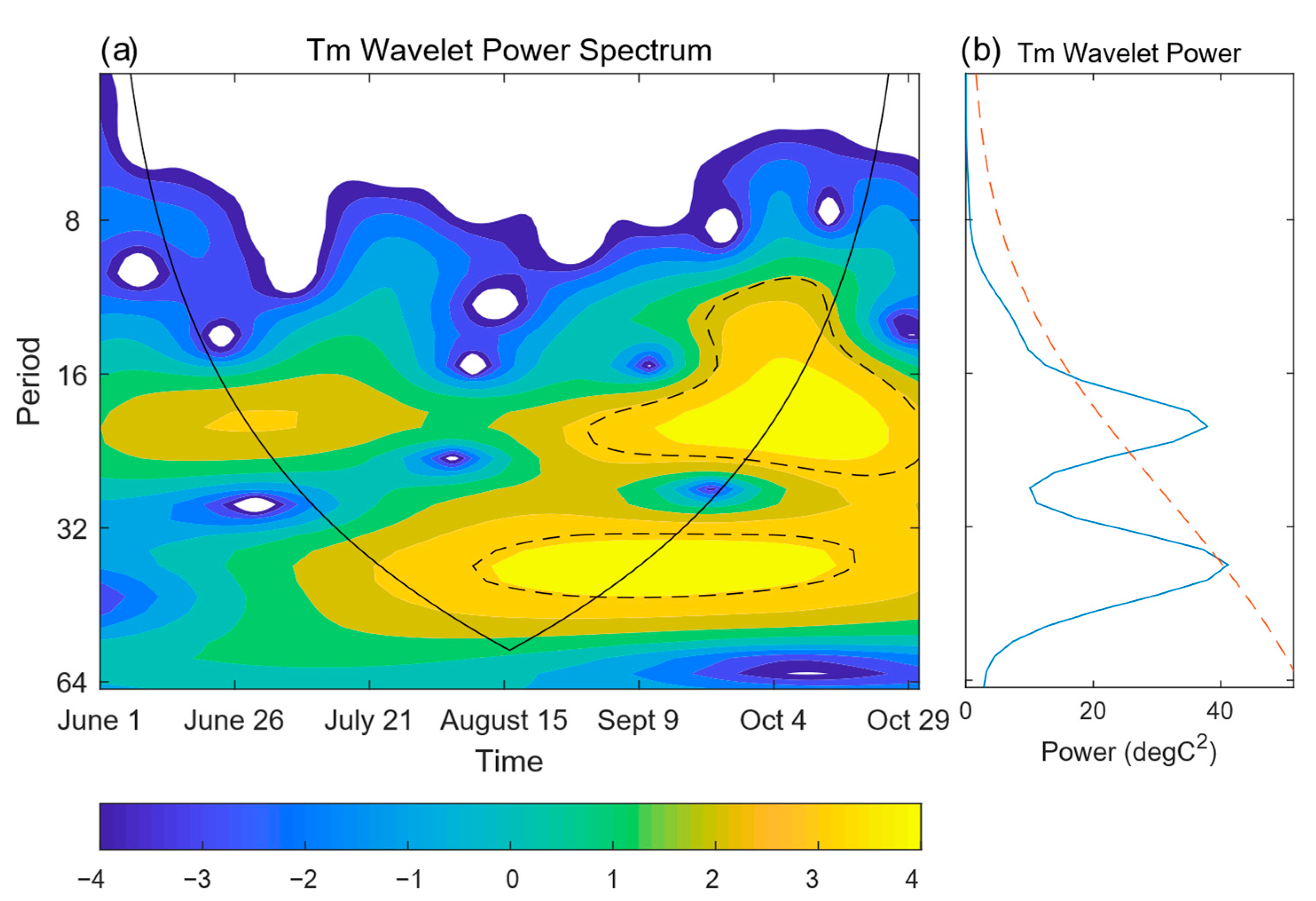
Figure 4 shows that the ISO signal of the area average 2 m temperature in summer 2022 had two obvious fluctuation periods of 10–30 and 32–48 days, and the periods passed the 95% significance test in the panel spectrum, showing obvious ISO characteristics. Nevertheless, only the 16–22-day range in the power spectrum passed the 95% significance test. Therefore, taking these two factors into consideration, we conclude that the ISO signal had a fluctuation period of 10–30 days. To study the influence of ISO signals on the CDHE, this event was divided into eight periods, in which P1–5 was the development period of the heatwave event, and the average maximum temperature in the region peaked at P5. In P4–8, drought events developed gradually, with moderate drought areas gradually expanding and peaking at P7. Therefore, the period during which the events were developing is the primary focus of our research. We defined P1–5 as the heatwave development period and P3–7 as the drought development period.
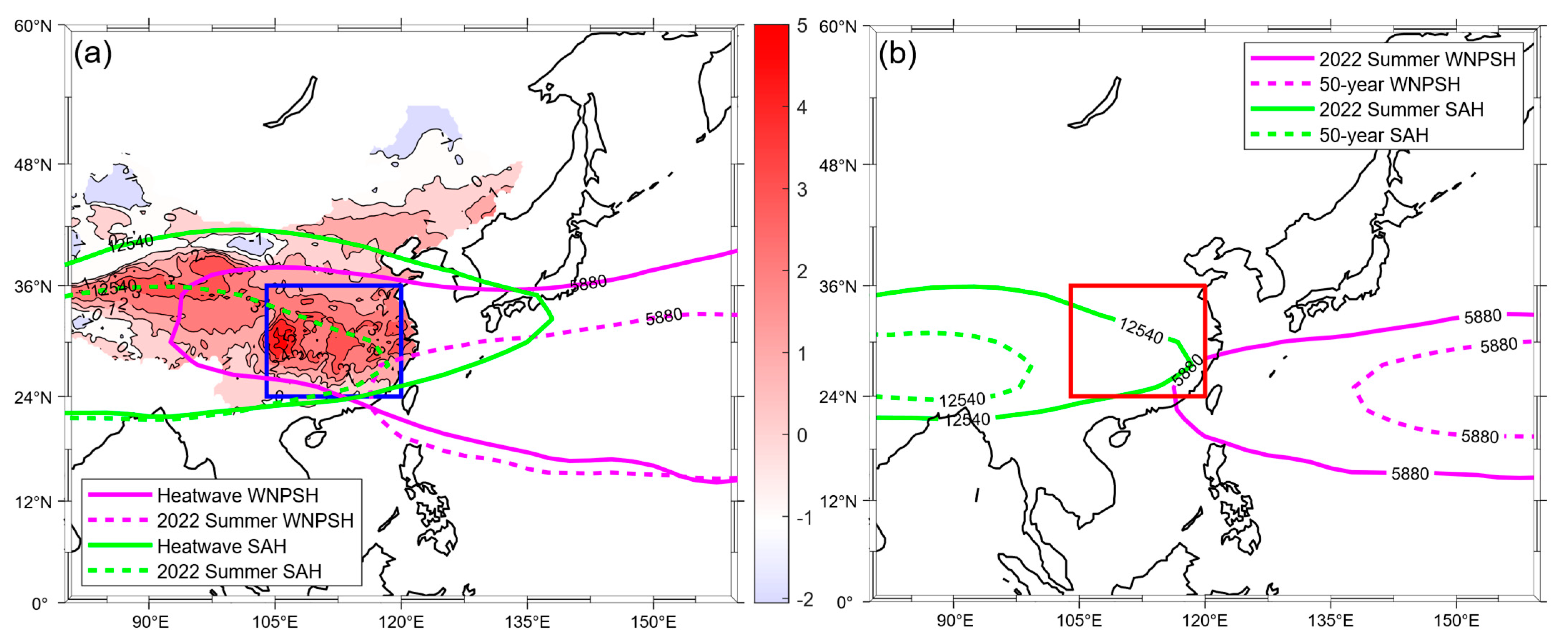
Figure 5a mainly shows the location of the SAH as well as the Western North Pacific subtropical high (WNPSH) during this heatwave episode and in the summer of 2022. During the heatwave event, WNPSH shifted dramatically westward from its average position in the summer of 2022, reaching as far as 93°E, covering most areas of southern China. At the same time, the eastward extension of SAH at 200 hPa was obvious, reaching as far as 138°E, affecting the MYRB, the Korean Peninsula, and parts of Japan. The combined effect of the two systems enhanced subsidence and divergence, resulting in the CDHE in the MYRB. In addition, we compared the summer average location in 2022 with the 50-year average location of SAH and WNPSH and found that the summer average location of SAH and WNPSH partially moved, but there was not much difference between the two (Figure 5b). In summary, it can be considered that the ISOs in the atmospheric circulation had an important impact on the occurrence and development of this CDHE, resulting in a long stay of SAH and WNPSH in summer in China, and playing a leading role in the occurrence of the temperature anomaly in the MYRB.
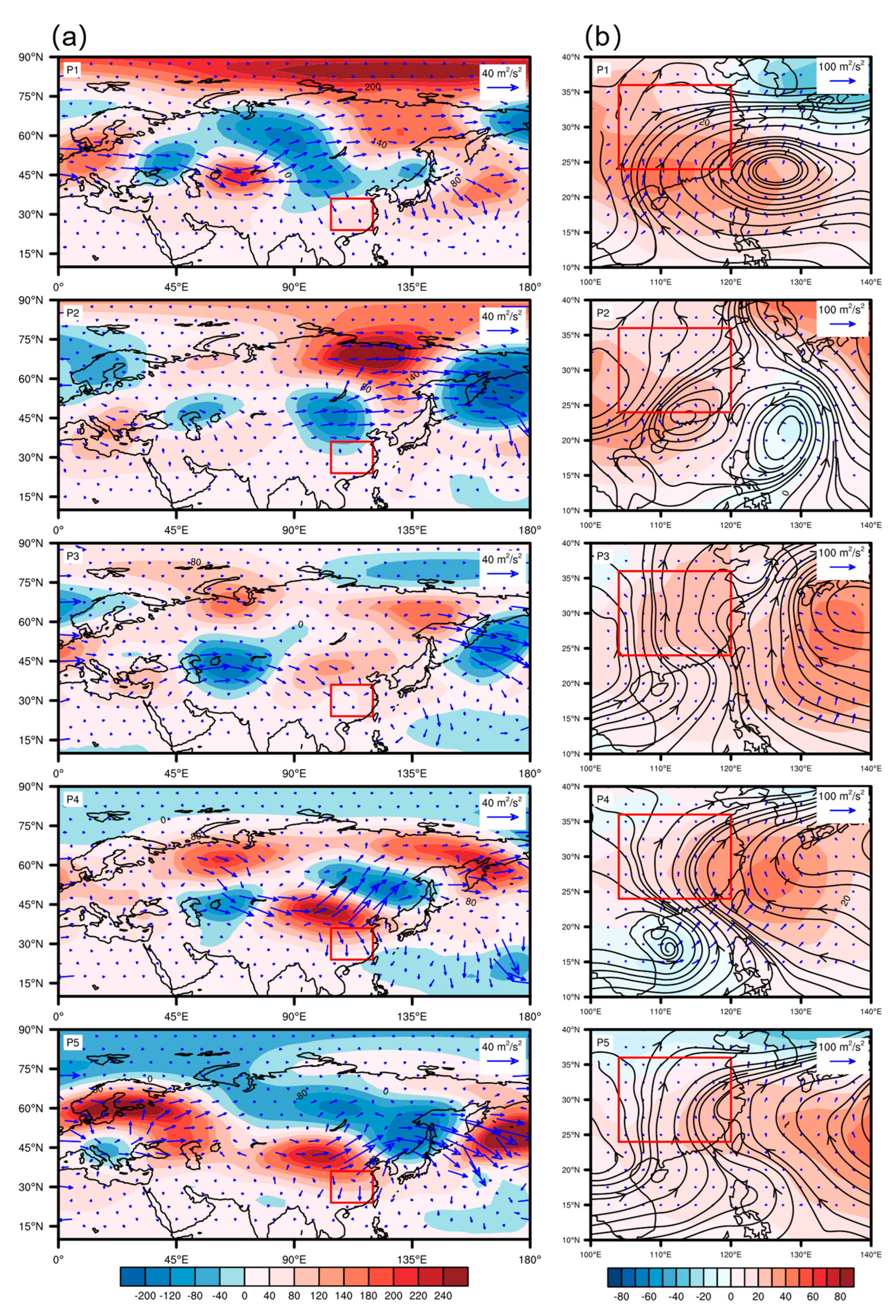
As shown in Figure 6, in P1–2, the MYRB was mainly affected by the negative geopotential height anomalous large value area in Mongolia at 200 hPa. In P3–5, the anomalous area gradually transformed into a positive anomaly, and the positive anomaly continued to intensify, causing the SAH to extend eastward, thereby controlling the MYRB. At the same time, there was always a series of positive and negative geopotential height anomalies in the midlatitude westerly wind belt above Eurasia at 200 hPa, having obvious wave series characteristics. The positive anomalous centers in the zonal wave series above Mongolia continued to affect the northern boundary of MYRB in P3–5, and the intensity of the anomalous centers increased significantly. At 800 hPa, the MYRB in P1–3 was affected by the positive anomaly and was dominated by the southerly with significant warm advection. In P4–5, the southern and eastern boundaries of the MYRB were constantly affected by the southeasterly anomaly, which transported negative vorticity over southern China. This further aggravated the positive geopotential height anomaly and was accompanied by wave fluxes transported northward. In the developing period of the heatwave event, the SAH and the WNPSH were coupled with each other and jointly controlled the MYRB so that the significant positive geopotential height anomaly stayed above the MYRB for a long period, which was conducive to the development of local subsidence.
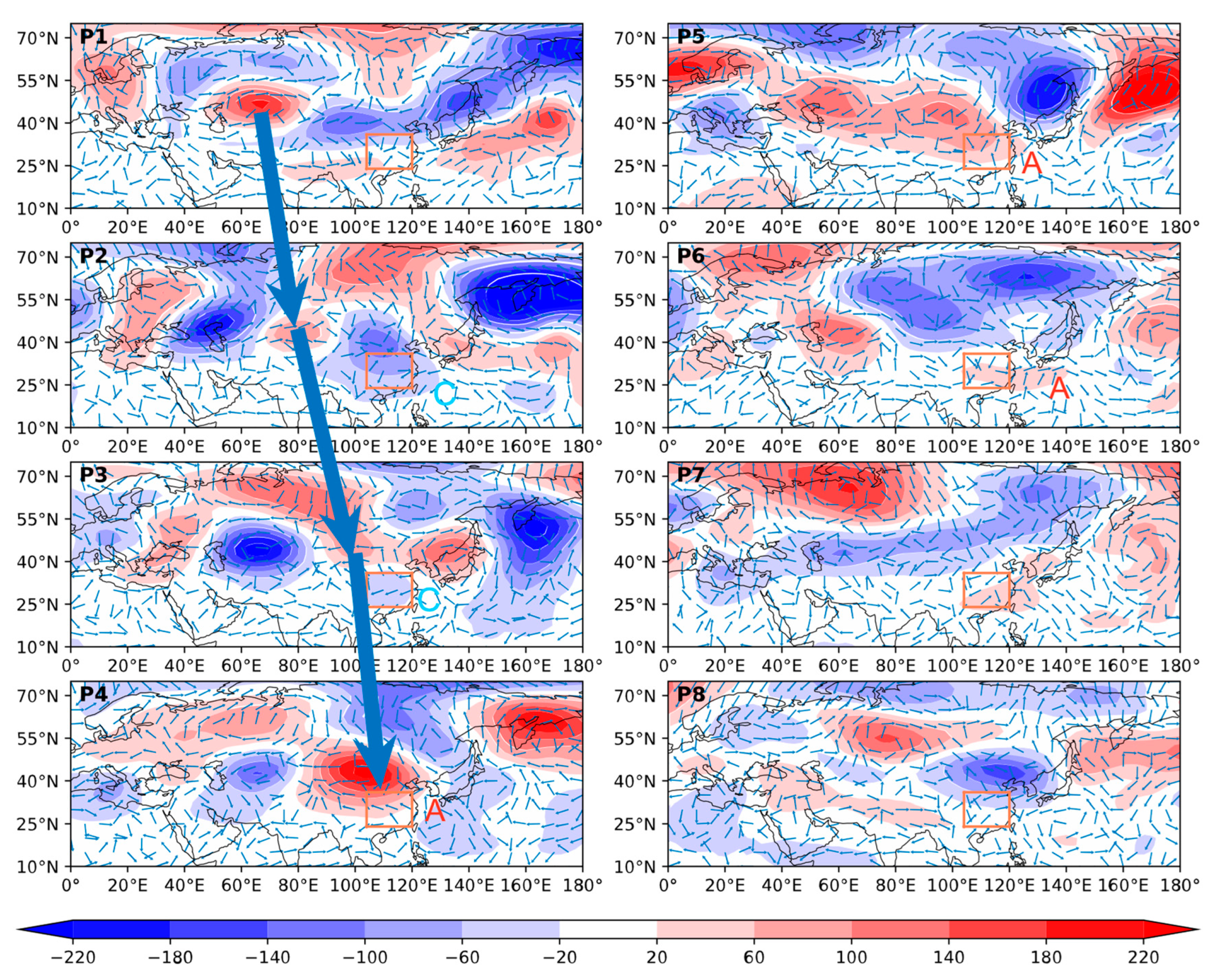
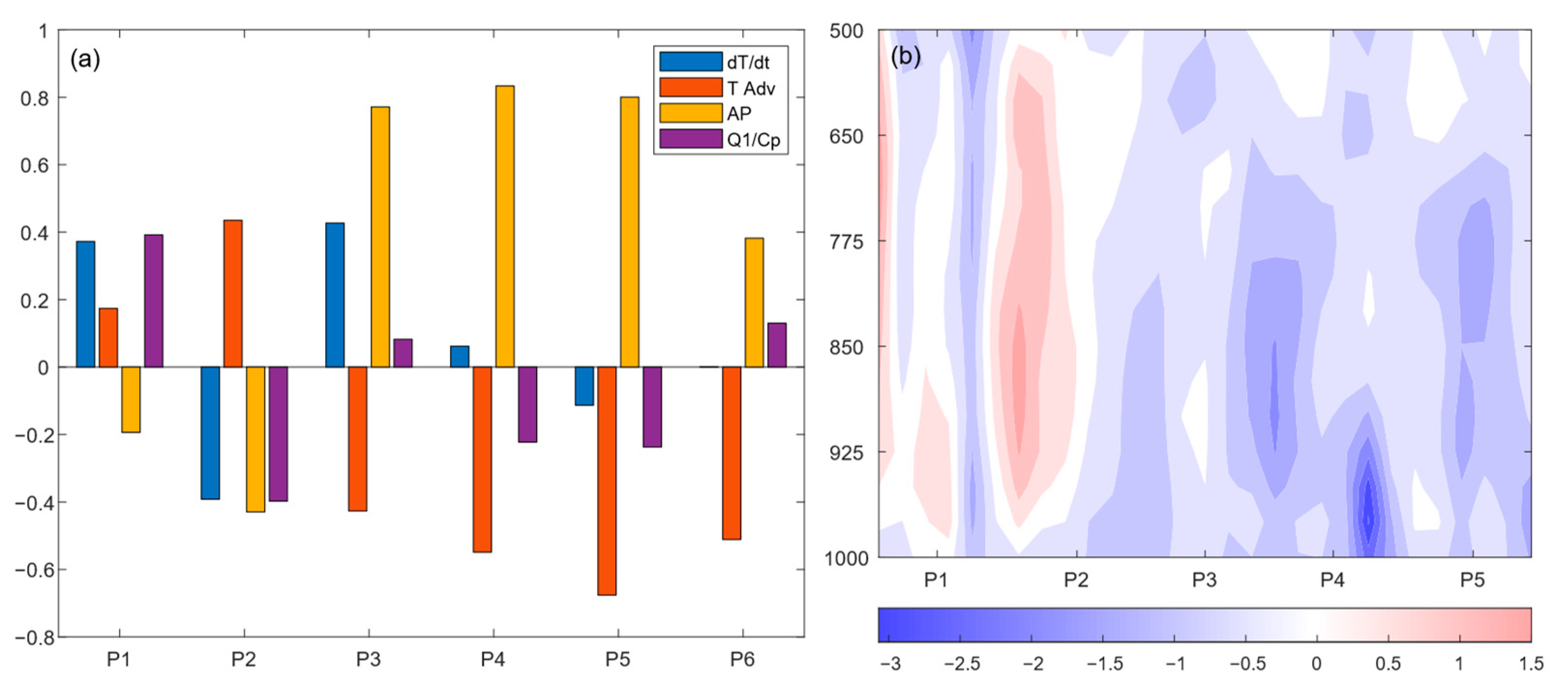
To further explore the evolution characteristics of ISOs in this event, we extracted the 10–30-day ISO components in the upper and lower troposphere, which are demonstrated in Figure 7. In P1–2, there was a significant negative geopotential height anomaly at 200 hPa above the MYRB, forming a strong cyclonic anomaly at 800 hPa in P2. According to Figure 8a, the local temperature of the MYRB oscillates due to the combined effect of the upper and lower troposphere. The temperature advection was positive at this time, transporting warm advection to the MYRB so that the local temperature rose (Figure 8b), laying the foundation for the occurrence of the heatwave event. In P3–4, the center of the positive geopotential height anomaly at 200 hPa gradually moved from Balkhash Lake toward the MYRB, so that the cyclonic anomaly at 800 hPa turned into an anticyclonic anomaly, continuously transporting negative vorticity into the MYRB. Anticyclone anomalies appeared simultaneously in both the upper and lower levels and produced continuous and stable subsidence. In this period, the positive geopotential height anomaly in the upper troposphere and the adiabatic heating brought by the lower troposphere (Figure 7a) played a leading role in the temperature budget, becoming the main trigger for rises in temperature. The positive anomaly center at 200 hPa in P5–6 gradually weakened, and the anticyclone anomaly at 800 hPa gradually moved away, with the temperature reaching the peak with only tiny changes (Figure 8a). In this period, the heatwave persisted for a long period of time, exacerbating the drought (Figure 3). In the last two periods, the positive geopotential height anomaly in the upper troposphere gradually transformed into a negative geopotential height anomaly, and the anticyclone anomaly in the lower level transformed into a cyclone anomaly. The temperature dropped sharply, and the heatwave event ended (Figure 3).
3.2. CDHE Evaluation for the Control
As was said before, a significant factor in this heatwave was a profound positive geopotential height anomaly over the whole troposphere. However, what are the effects of the circulation anomaly with a wave train characteristic from middle and high latitudes at 200 hPa and the ISO fluctuations from the tropical area at 800 hPa on the MYRB, and how much did they contribute to the heatwave event in different regions? To answer the above questions, PLF experiments were introduced into this study to simulate atmospheric evolutions over southern China when different signals were absent.
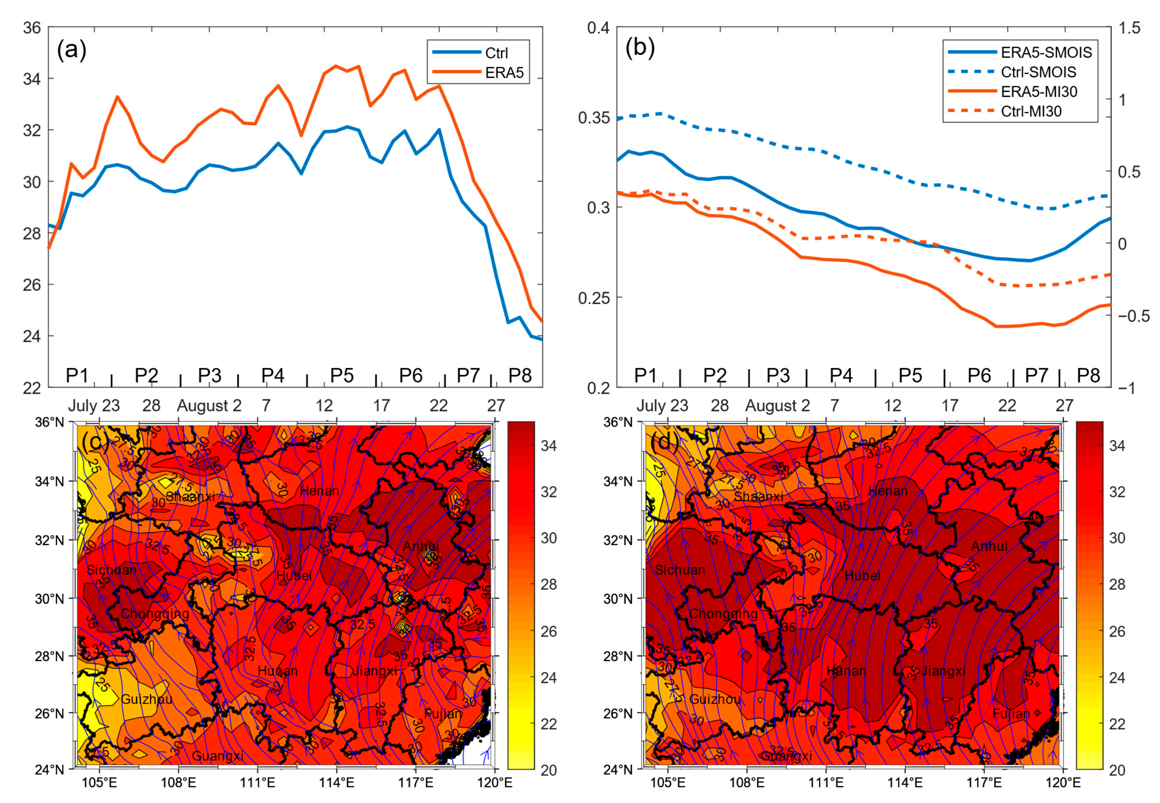
Comparing the time series of average maximum temperature in the MYRB of the control run and the reanalysis data (Figure 9a), the trend and the fluctuations of temperature series in the control run were basically consistent with those of the reanalysis data, but the amplitude was reduced by 2–3 °C on average. Figure 9b shows that the soil moisture in both the control run and the reanalysis data continued to decrease during the event and rebounded around 25 August, and the difference in the amplitude of the MI30 index between the control run and the actual data was not obvious. The simulation results were basically consistent with the actual situation. Figure 9c,d show the maximum ground temperature of the control run and the reanalysis data, respectively. The heatwave event mainly occurred in the Sichuan Basin and the central and eastern parts of the region. The control run basically demonstrated the distribution of the area with a maximum temperature above 35 °C, but the simulation ability in the southern part of the region was weak (Figure 9c). According to the wind field in the MYRB at 850 hPa, the results of the control run were quite similar to the reanalysis data, showing that the area was mainly controlled by the southerly. During the heatwave event, the drought level gradually rose, and by 24 August, the stations with a light drought or more severe reached 85.15%, and the stations with a moderate drought or more severe reached 67.55%.
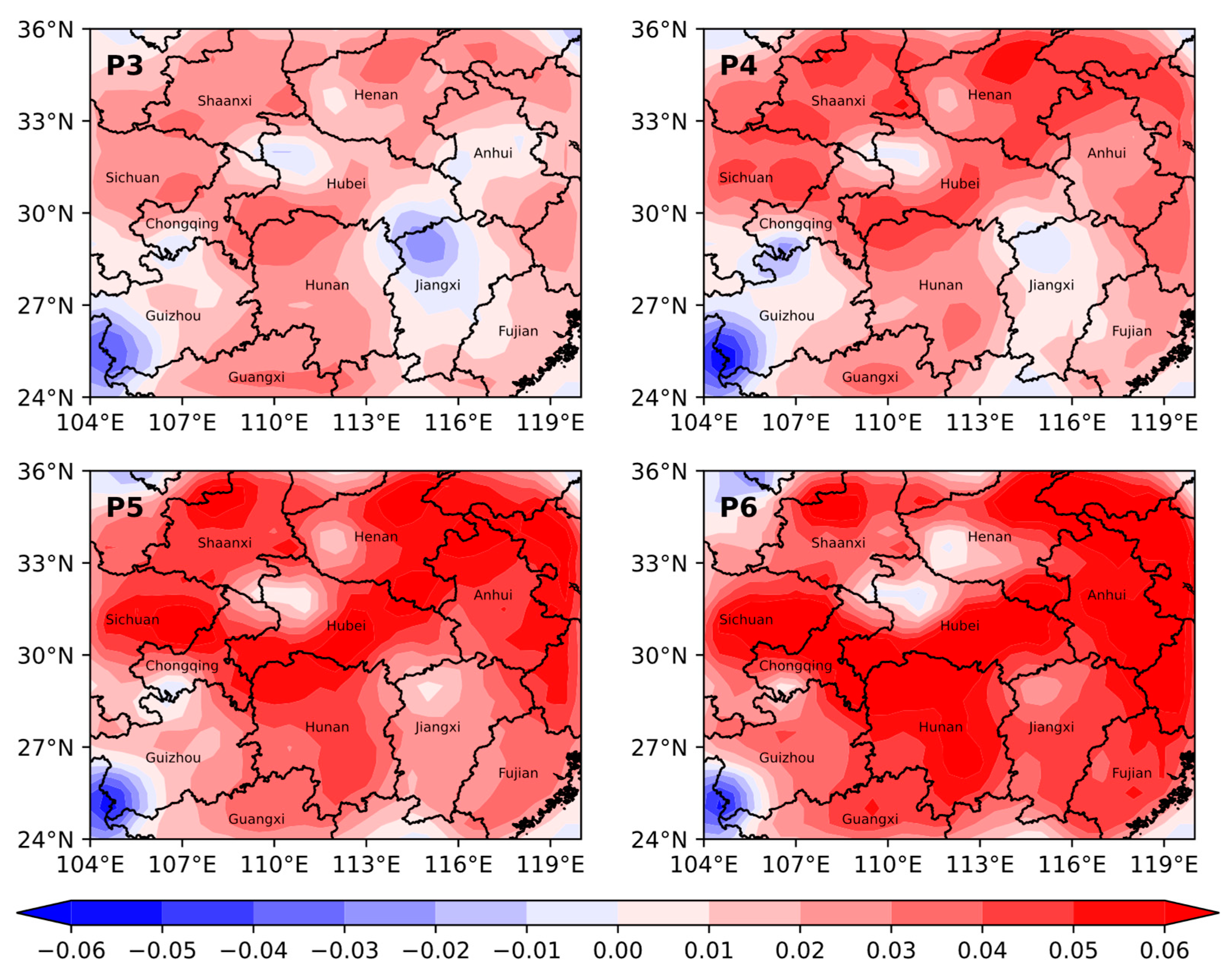
Compared with P1, the soil moisture in most areas in the MYRB in P3-6 decreased significantly with time, except at the junction of Guizhou Province and Yunnan Province, and the maximum decrease reached 0.06 (Figure 10). The continuous soil moisture decline was also consistent with the decline in MI30 shown in Figure 9b, reflecting the wide range of this event. In summary, it can be considered that the control run can simulate the CDHE in the MYRB well.
3.3. ISOs’ Influence on the CDHE in PLF Trials
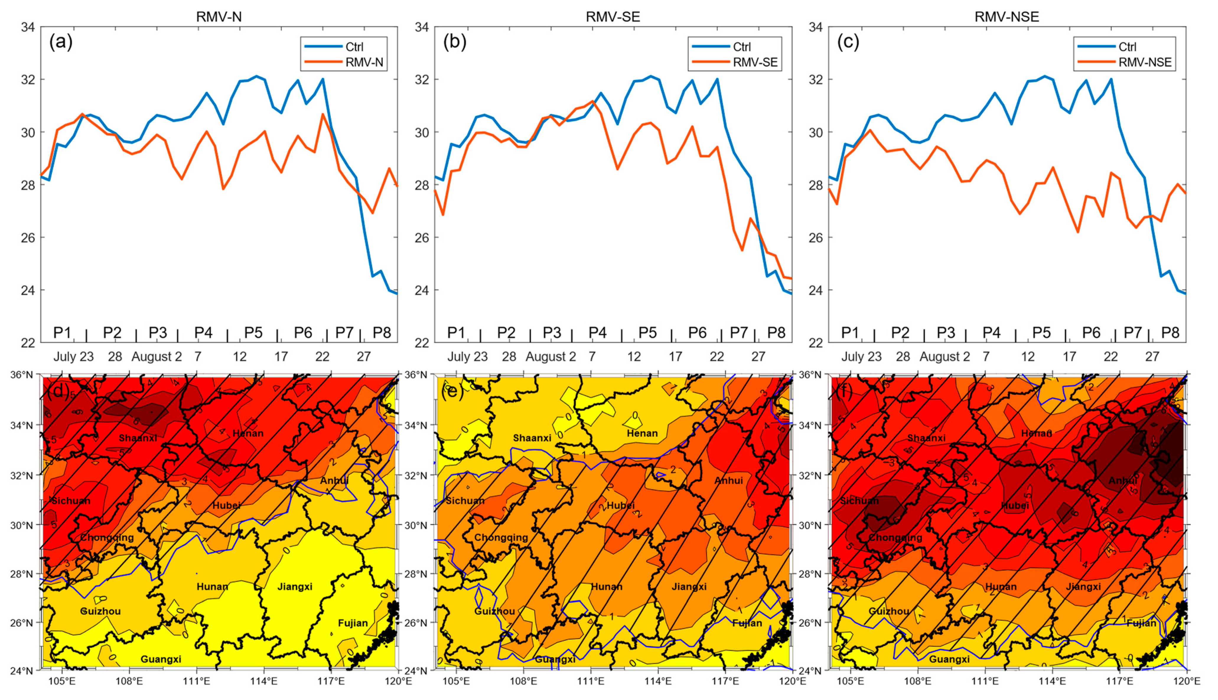
To obtain the influence of different ISO signals from extratropical and tropical areas on the CDHE, three PLF experiments were performed, including RMV-N, RMV-SE, and RMV-NSE. Comparing the results of the sensitive runs with the control run, it was found that the area average maximum temperature in all sensitive runs decreased to a certain extent, but the levels of the decrease were significantly different. At the beginning part of the event (19 July–3 August), the removal of ISO signals on all three boundaries did not have a significant impact on the area average maximum temperature. However, when the event entered the late period (P3–P5), the ISO first affected the northern boundary of the MYRB (Figure 11a) and began to affect the south and east boundaries of the MYRB on 9 August (Figure 11b). After that, the impact of the extratropical ISO ended earlier than the tropical ISO signal. In P5, the area average temperature difference between the control run and the RMV-N and RMV-SE runs reached 2.4 °C and 1.93 °C, respectively. As shown in Figure 11d,e, during the heatwave event, the influence of the extratropical ISO mainly concentrated in the northwestern part of the study area, and the southern part of Shaanxi Province showed the most significant difference. The maximum cooling amplitude was more than 6 °C. The impact of the tropical ISO was mainly concentrated in the central and eastern parts, and the maximum cooling amplitude was more than 5 °C. Comparing the temperature changes in the two runs, it can be concluded that the influence of the extratropical ISO was greater than that of the tropical ISO. As shown in Figure 11c, after removing the ISO signals from all three boundaries at the same time, the area average maximum temperature dropped significantly, and the maximum cooling amplitude was more than 7 °C, with a wider range of influence (Figure 11f). The combined effect of the two ISOs had a conspicuous impact on this hot event.
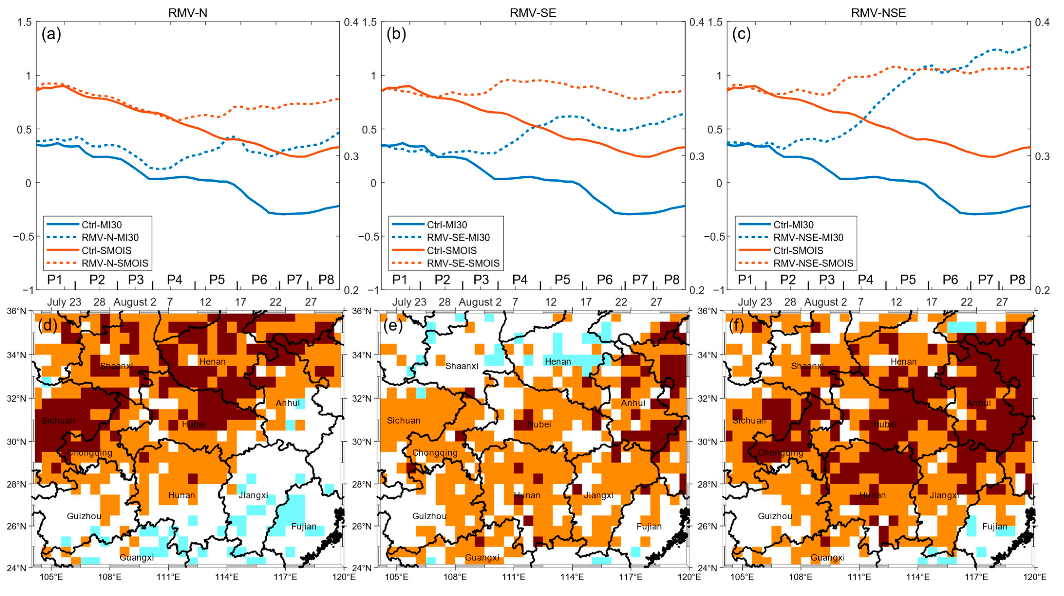
As the heatwave event developed, it also caused a wide range of drought events. Figure 12a–c shows the comparison of the MI30 index and the soil moisture between the three sensitive runs and the control run in turn. When the ISO signal from the northern boundary is removed (Figure 12a), it can be seen that the MI30 index and the soil moisture had a significant rise after 3 August, and the gap between the two runs increased over time. Figure 12d shows that most areas in the MYRB had a declining drought level in P6–7, and the significant declining area mainly concentrated in the Sichuan Basin and the junction of Henan and Hubei Provinces. Most grids north of 28°N had one level declined (34.06% of the total grids), and the proportion of grids having two levels declined was 19.64%. When the ISO signal from the southern and eastern boundaries was removed, the increasing trends of the MI30 index and soil moisture were consistent with those in the RMV-N run (Figure 12b). From the change in drought level in P6–7 (Figure 12e), we can see that the significant declining area mainly lay in the northeastern part of the MYRB, but the number of grids with two levels declined was less than that in the RMV-N run, accounting for only 7.64% of the total grids. There were more grids with one level declined (42.06% of the total grids), which showed that this drought event was more affected by the extratropical ISO signal. After removing ISO signals from all three boundaries (Figure 12c,f), the MI30 index increased significantly. From 3 August to 19 August, the MI30 index increased by an average of 1.36 compared with the control run, and the soil moisture increased the most in all sensitive runs by 0.059 . Correspondingly, the area with a declining drought level expanded significantly, with a greater decline in most grids. Grids with one level declined accounted for 41.33% of the total, and grids with two levels declined accounted for 28.12%. In summary, the CDHE was more affected by the extratropical ISO signal, and the combined effect of two ISO signals jointly promoted this complex and serious CDHE.
To gain further insight into the effect of ISOs on this CDHE, in Figure 13, the difference in several meteorological elements between the control run and the RMV-NSE run is shown. As shown in Figure 11a, in the late stage of the development of the heatwave event (P3–5), the adiabatic heating decreased after removing the ISO components, leading to a continuous temperature decrease in the MYRB and proving that the heatwave was mainly caused by the ISO component. Figure 13b,c show that in P1 in the control run, no sign of convergence or divergence was shown in the lower troposphere, and the upper troposphere was dominated by positive horizontal divergence. As time passed, the lower troposphere became divergent, and the upper layer became convergent, with airflow transported from the upper level to the lower level. This top-down “pumping effect” caused consistent subsidence in the troposphere. At the same time, there was a close relationship between the vertical velocity and the horizontal divergence. As shown in Figure 13c, in the control run in P1, the upper troposphere was mainly dominated by upward airflow, and the lower troposphere was dominated by downward airflow. As time went by, the vertical movement in the upper level of the MYRB gradually turned from upward movement to downward movement under the influence of ISO signals, and the velocity of the lower subsidence increased. Taking the filled contour map into consideration, it can be seen that if there was no ISO influencing, the atmosphere status in both upper and lower levels would not change much in P3–5, so the ISO signal had a very significant promotion effect on the subsidence. It contributed to forming a continuous and stable downward movement and intensifying the atmospheric subsidence warming effect. The specific analysis of each layer in P3–5 is shown in Figure 13d–f. In the area north of 28°N in the MYRB at 200 hPa, there was a significant positive geopotential height anomalous area, and the anomaly gradually intensified with the increase in latitude, reflecting that the eastward shift of the SAH mainly affected the northern part of the MYRB, which is also consistent with the results shown in Figure 13a. As the WNPSH pushed positive geopotential height anomaly westward at 500 hPa, it effectively covered the entire MYRB. Although the difference in geopotential height at 800 hPa was smaller than that at 200 and 500 hPa, it also showed a significant positive anomaly. In short, the ISO caused the geopotential height of the entire troposphere to rise, accompanied by the “pumping effect” of the convergence in the upper troposphere and the divergence in the lower troposphere, causing regional subsidence over the MYRB and the occurrence of this CDHE.
4. Conclusions
In this paper, the influence mechanism of ISO signals from extratropical and tropical areas on a CDHE in the MYRB in the summer of 2022 was analyzed. During this event, the wave series forming in the upper troposphere at 200 hPa played a significant role in the occurrence of the CDHE in the northern part of the MYRB. By comparing the results of the RMV-N run and the control run, it was found that the ISO component of the northern boundary caused the mean temperature to rise by 2.4 °C and aggravated the drought in 53.7% of the region.
At the same time, the anticyclonic anomaly in the lower troposphere at 800 hPa had a continuous impact on the southern and eastern boundaries. By comparing the results of the RMV-SE run and the control run, it was found that the ISO component of these two boundaries can increase the average temperature by 1.93 °C in the MYRB and intensify the drought in 49.7% of the area. The influence of the tropical ISO was weaker than that of the extratropical ISO, but the two ISO signals were coupled with each other, and the combined effect contributed to this severe CDHE together. By comparing the results of the RMV-NSE run and the control run, it was found that the combined ISO components can increase the average temperature by 3.91 °C in the MYRB and exacerbated the drought degree in 69.45% of the region.
Therefore, under the combined effect of the above ISOs, the temperature increase in the MYRB in the late period of the event was mainly caused by adiabatic heating, together with the “pumping effect” through the whole troposphere forming a continuous and stable subsidence, reducing the occurrence of precipitation and other weather. After the heatwave event reached its peak, the high temperature began to drop rapidly, and the drought began to become serious.
This paper quantifies the extent to which ISOs from both tropical and mid-latitudes affect a persistent drought and hot disaster in the MYRB by designing PLF experiment. However, the ISOs at different latitudes were not distinguished and might have interactions between them [44]. Compound and interactive effects of ISOs from different latitudes deserve further exploration. Therefore, in future studies, the causes and developments of regional weather extremes can be investigated by analyzing the combined effects of different ISOs. In addition, in this study the northern, southern, and eastern boundaries of the MYRB are considered to be affected by the ISOs. As the source of the Yangtze River lies in the Tibetan Plateau, the ISO fluctuations from the Tibetan Plateau can also affect the weather conditions in the MYRB [45]. To further improve this study, we could take into consideration the influence of the ISO from the Tibetan Plateau on the western boundary.
Author Contributions
Conceptualization, Y.Q. (Yi Qin) and Y.Q. (Yujing Qin); methodology, Y.S.; validation, Y.Q. (Yujing Qin), Y.L. and B.X.; writing—original draft preparation, Y.Q. (Yi Qin) and Y.S.; supervision, Y.Q. (Yujing Qin) All authors have read and agreed to the published version of the manuscript.
Funding
This research was funded by the Jiangsu Provincial Key R&D Program (Grant No. BE2022161), Special Program for Innovation and Development of China Meteorological Admin-istration (Grant No. CXFZ2022J031) and the National Natural Science Foundation of China, grant number (Grant No. 41875111).
Data Availability Statement
The ECMWF (https://cds.climate.copernicus.eu/, accessed on 12 November 2022) and MODIS (https://lpdaac.usgs.gov/products/mod13c1v006/, accessed on 7 December 2022) data used in this study are freely available.
Acknowledgments
The authors gratefully acknowledge NASA and ECMWF for their effort in making the data available.
Conflicts of Interest
The authors declare no conflict of interest.
References
- IPCC. Climate Change 2021: The Physical Science Basis. In Contribution of Working Group I to the Sixth Assessment Report of the Intergovernmental Panel on Climate Change; Cambridge University Press: Cambridge, UK, 2021; p. 8. [Google Scholar]
- Zhang, H.; Wang, E.L.; Zhou, D.W.; Luo, Z.K.; Zhang, Z.X. Rising soil temperature in china and its potential ecological impact. Sci. Rep. 2016, 6, 8. [Google Scholar] [CrossRef]
- Lu, Y.; Hu, H.; Li, C.; Tian, F. Increasing compound events of extreme hot and dry days during growing seasons of wheat and maize in China. Sci. Rep. 2018, 8, 16700. [Google Scholar] [CrossRef]
- Jiang, W.X.; Wang, L.C.; Feng, L.; Zhang, M.; Yao, R. Drought characteristics and its impact on changes in surface vegetation from 1981 to 2015 in the Yangtze River Basin, China. Int. J. Climatol. 2020, 40, 3380–3397. [Google Scholar] [CrossRef]
- Kong, Q.; Guerreiro, S.B.; Blenkinsop, S.; Li, X.-F.; Fowler, H.J. Increases in summertime concurrent drought and heatwave in Eastern China. Weather Clim. Extrem. 2020, 28, 100242. [Google Scholar] [CrossRef]
- Luo, M.; Lau, N.C. Amplifying effect of ENSO on heat waves in China. Clim. Dyn. 2019, 52, 3277–3289. [Google Scholar] [CrossRef]
- Gao, T.; Luo, M.; Lau, N.C.; Chan, T.O. Spatially Distinct Effects of Two EL Nino Types on Summer Heat Extremes in China. Geophys. Res. Lett. 2020, 47, 9. [Google Scholar] [CrossRef]
- Wei, J.; Wang, W.G.; Shao, Q.X.; Yu, Z.B.; Chen, Z.F.; Huang, Y.; Xing, W.Q. Heat wave variations across China tied to global SST modes. J. Geophys. Res.-Atmos. 2020, 125, 22. [Google Scholar] [CrossRef]
- Cao, D.R.; Xu, K.; Huang, Q.L.; Tam, C.Y.; Chen, S.; He, Z.Q.; Wang, W.Q. Exceptionally prolonged extreme heat waves over South China in early summer 2020: The role of warming in the tropical Indian Ocean. Atmos. Res. 2022, 278, 11. [Google Scholar] [CrossRef]
- Chen, R.D.; Wen, Z.P.; Lu, R.Y. Large-Scale Circulation Anomalies and Intraseasonal Oscillations Associated with Long-Lived Extreme Heat Events in South China. J. Clim. 2018, 31, 213–232. [Google Scholar] [CrossRef]
- Hong, J.L.; Ke, Z.J.; Yuan, Y.; Shao, X. Boreal Summer Intraseasonal Oscillation and Its Possible Impact on Precipitation over Southern China in 2019. J. Meteorol. Res. 2021, 35, 571–582. [Google Scholar] [CrossRef]
- Chen, J.P.; Wen, Z.P.; Wu, R.G.; Chen, Z.S.; Zhao, P. Influences of northward propagating 25–90-day and quasi-biweekly oscillations on eastern China summer rainfall. Clim. Dyn. 2015, 45, 105–124. [Google Scholar] [CrossRef]
- Chen, R.D.; Wen, Z.P.; Lu, R.Y. Evolution of the Circulation Anomalies and the Quasi-Biweekly Oscillations Associated with Extreme Heat Events in Southern China. J. Clim. 2016, 29, 6909–6921. [Google Scholar] [CrossRef]
- Ding, T.; Ke, Z.J. Characteristics and changes of regional wet and dry heat wave events in China during 1960–2013. Theor. Appl. Climatol. 2015, 122, 651–665. [Google Scholar] [CrossRef]
- Hsu, P.C.; Lee, J.Y.; Ha, K.J.; Tsou, C.H. Influences of Boreal Summer Intraseasonal Oscillation on Heat Waves in Monsoon Asia. J. Clim. 2017, 30, 7191–7211. [Google Scholar] [CrossRef]
- Lu, X.J.; Fang, J.B.; Yang, X.Q.; Hu, H.B. Intra-seasonal summer precipitation anomaly over eastern China and evolution characteristics of its associated tropical and mid-to-high latitudes atmospheric circulation. Acta Meteorol. Sin. 2022, 80, 1–20. (In Chinese) [Google Scholar] [CrossRef]
- Rummukainen, M. Added Value in Regional Climate Modeling; Wiley Interdiscip: Hoboken, NJ, USA, 2016; Volume 7, pp. 145–159. [Google Scholar]
- Hu, W.T.; Duan, A.M.; Li, Y.; He, B. The Intraseasonal Oscillation of Eastern Tibetan Plateau Precipitation in Response to the Summer Eurasian Wave Train. J. Clim. 2016, 29, 7215–7230. [Google Scholar] [CrossRef]
- Shi, H.; Yu, J.H.; Wang, C.X.; Qiu, Z.D. Influence of boreal summer intraseasonal oscillation on tropical cyclone heavy rain in southeastern coast China. J. Meteorol. Sci. 2018, 38, 11–18. (In Chinese) [Google Scholar] [CrossRef]
- NDRCC: Basic Situation of Natural Disasters in August 2022. Available online: http://www.ndrcc.org.cn/zqtj/27015.jhtml (accessed on 28 October 2022).
- Yang, H.; Wang, B. Multiscale processes in the genesis of a near-equatorial tropical cyclone during the Dynamics of the MJO Experiment: Results from partial lateral forcing experiments. J. Geophys. Res. D Atmos. 2018, 123, 5020–5037. [Google Scholar] [CrossRef]
- Hersbach, H.; Bell, B.; Berrisford, P.; Hirahara, S.; Horanyi, A.; Munoz-Sabater, J.; Nicolas, J.; Peubey, C.; Radu, R.; Schepers, D.; et al. The ERA5 global reanalysis. Q. J. R. Meteorol. Soc. 2020, 146, 1999–2049. [Google Scholar] [CrossRef]
- Huang, S.; Tang, L.N.; Hupy, J.P.; Wang, Y.; Shao, G.F. A commentary review on the use of normalized difference vegetation index (ndvi) in the era of popular remote sensing. J. For. Res. 2021, 32, 1–6. [Google Scholar] [CrossRef]
- Didan, K. MOD13C1 MODIS/Terra Vegetation Indices 16-Day L3 Global 0.05Deg CMG V006; NASA EOSDIS Land Processes DAAC: Sioux Falls, SD, USA, 2015. [CrossRef]
- Jayakumar, D.; Sathish, K.D.; Thendiyath, R. Integrating Disaster Science and Management; Elsevier Science: Amsterdam, The Netherland, 2018; ISBN 978-0-12-812056-9. [Google Scholar]
- Qi, X.; Yang, J. Extended-range prediction of a heat wave event over the Yangtze River Valley: Role of intraseasonal signals. J. Geo-Phys. Res. Atmos. 2019, 12, 451–457. [Google Scholar] [CrossRef]
- Xie, W.S.; Zhang, Q.; Li, W.; Wu, B.W. Analysis of the Applicability of Drought Indexes in the Northeast, Southwest and Middle-lower Reaches of Yangtze River of China. Plateau Meteorol. 2021, 40, 1136–1146. (In Chinese) [Google Scholar] [CrossRef]
- GB/T 20481-2017; Grades of Meteorological Drought. International Organization for Standardization: Beijing, China, 2017.
- Thornthwaite, C.W. An approach toward a rational classification of climate. Soil Sci. 1948, 66, 77. [Google Scholar] [CrossRef]
- Yanai, M.; Esbensen, S.; Chu, J.H. Determination of bulk properties of tropical cloud clusters from large-scale heat and moisture budgets. J. Atmos. Sci. 1973, 30, 611–627. [Google Scholar] [CrossRef]
- Wang, L.J.; Dai, A.G.; Guo, S.H.; Ge, J. Establishment of the south asian high over the indo-china peninsula during late spring to summer. Adv. Atmos. Sci. 2017, 34, 169–180. [Google Scholar] [CrossRef]
- Lu, C.H.; Shen, Y.C.; Li, Y.H.; Xiang, B.; Qin, Y.J. Role of intraseasonal oscillation in a compound drought and heat event over the middle of the yangtze river basin during midsummer 2018. J. Meteorol. Res. 2022, 36, 643–657. [Google Scholar] [CrossRef]
- Shi, C.H.; Jin, X.; Liu, R.Q. The differences in characteristics and applicability among three types of Rossby wave activity flux in atmospheric dynamics. Trans. Atmos. Sci. 2017, 40, 850–855. (In Chinese) [Google Scholar] [CrossRef]
- Takaya, K.; Nakamura, H. A formulation of a phase-independent wave-activity flux for stationary and migratory quasigeostrophic eddies on a zonally varying basic flow. J. Atmos. Sci. 2001, 58, 608–627. [Google Scholar] [CrossRef]
- Skamarock, W.C.; Klemp, J.B.; Dudhia, J.; Gill, D.O.; Liu, Z.; Berner, J.; Wang, W.; Powers, J.G.; Duda, M.G. A Description of the Advanced Research WRF Version 4; NCAR Tech. Note NCAR/TN-556+STR; National Center for Atmospheric Research: Boulder, CO, USA, 2019; 145p. [Google Scholar] [CrossRef]
- Hong, S.Y.; Dudhia, J.; Chen, S.H. A revised approach to ice microphysical processes for the bulk parameterization of clouds and precipitation. Mon. Weather Rev. 2004, 132, 103–120. [Google Scholar] [CrossRef]
- Collins, W.; Rasch, P.; Boville, B.; McCaa, J.; Williamson, D.; Kiehl, J.; Briegleb, B.; Bitz, C.; Lin, S.-J.; Zhang, M.; et al. Description of the NCAR Community Atmosphere Model (CAM 3.0); NCAR Tech. Note NCAR/TN-464+STR; University Corporation for Atmospheric Research: Boulder, CO, USA, 2004; 214p. [Google Scholar]
- Janjić, Z.I. Nonsingular Implementation of the Mellor–Yamada Level 2.5 Scheme in the NCEP Meso Model; NCEP Office Note; National Centers for Environmental Prediction: College Park, MD, USA, 2002; 61p.
- Chen, F.; Dudhia, J. Coupling an advanced land surface–hydrology model with the Penn State–NCAR MM5 modeling system. Part I: Model implementation and sensitivity. Mon. Weather Rev. 2001, 129, 569–585. [Google Scholar] [CrossRef]
- Janjić, Z.I. The step-mountain eta coordinate model: Further developments of the convection, viscous sublayer, and turbulence closure schemes. Mon. Wea. Rev. 1994, 122, 927–945. [Google Scholar] [CrossRef]
- Janjić, Z.I. Comments on “Development and evaluation of a convection scheme for use in climate models”. J. Atmos. Sci. 2000, 57, 3686. [Google Scholar] [CrossRef]
- Yang, H.W.; Wang, B. Partial lateral forcing experiments reveal how multi-scale processes induce devastating rainfall: A new application of regional modeling. Clim. Dyn. 2015, 45, 1157–1167. [Google Scholar] [CrossRef]
- Xukai, Z.; Rong, G.; Xianyan, C.; Ling, W.; Wei, L.; Wenting, G.; Qiang, Z. Monitoring and assessment of summer drought in the Yangtze River basin in 2022. China Flood Drought Manag. 2022, 32, 12–16. (In Chinese) [Google Scholar] [CrossRef]
- Joseph, S.; Sahai, A.K.; Chattopadhyay, R.; Goswami, B.N. Can El Niño–Southern Oscillation (ENSO)events modulate intraseasonal oscillations of Indian summer monsoon? J. Geophys. Res. 2011, 116, D20123. [Google Scholar] [CrossRef]
- Yang, L.Y.; Wang, S.Y.; Fu, C.B. The Review of the Influence of Sub-Seasonal Oscillation on Precipitation over the Qinghai-Xizang (Tibetan) Plateau and its Downstream East Asian Monsoon Region. Plateau Meteorol. 2021, 40, 1432–1442. (In Chinese) [Google Scholar] [CrossRef]
Figure 1.
The terrain condition of South China (shading; m). The white dots mark the stations whose MCI data are used in this study.
Figure 1.
The terrain condition of South China (shading; m). The white dots mark the stations whose MCI data are used in this study.

Figure 2.
Climatology (2000–2021) NDVI in early (a) and late (d) August, NDVI in 2022 in early (b) and late (e) August and the differences between them ((c) for early August and (f) for late August).
Figure 2.
Climatology (2000–2021) NDVI in early (a) and late (d) August, NDVI in 2022 in early (b) and late (e) August and the differences between them ((c) for early August and (f) for late August).

Figure 3.
Area average maximum temperature () time series from 19 July to 31 August (blue bars; °C) with the red line denoting its 5-day moving average and the percentage of stations having a moderate drought or a more severe condition (MCI less than −1.0) (orange bars; %).
Figure 3.
Area average maximum temperature () time series from 19 July to 31 August (blue bars; °C) with the red line denoting its 5-day moving average and the percentage of stations having a moderate drought or a more severe condition (MCI less than −1.0) (orange bars; %).

Figure 4.
Wavelet analysis results of the ISO component of the anomaly, with wavelet spectrum (a) shown in the left panel and power spectrum (b) in the right panel. Dashed lines in both panels indicates that the results passed the 95% significant test. The black line denotes the cone of influence; everything outside it is ignored.

Figure 5.
(a) Mean location of SAH (green solid line) and WNPSH (pink solid line) and temperature anomaly during the heatwave event (shading; °C) compared with the 2022 summer average location of SAH (green dashed line) and WNPSH (pink dashed line). (b) The 2022 summer mean location of SAH (green solid line) and WNPSH (pink solid line) compared with the climatology locations (dashed lines). The location of SAH is marked by the 12,540 gpm line in 200 hPa and the location of the WNPSH is marked by the 5880 gpm line in 500 hPa. The red and blue box marks South China.

Figure 6.
(a) TN wave flux (vectors; ) and geopotential height anomalies (shading; gpm) in P1–5 at 200 hPa. (b) TN wave flux (vectors; ), geopotential height anomalies (shading; gpm), and wind anomalies (streamlines; ) in P1–5 at 800 hPa. The red box marks South China.
Figure 6.
(a) TN wave flux (vectors; ) and geopotential height anomalies (shading; gpm) in P1–5 at 200 hPa. (b) TN wave flux (vectors; ), geopotential height anomalies (shading; gpm), and wind anomalies (streamlines; ) in P1–5 at 800 hPa. The red box marks South China.

Figure 7.
ISO component of geopotential height (shading; gpm) at 200 hPa and wind (vectors; ) at 800 hPa in P1–8. A and C mark the anticyclonic and cyclonic wind anomalies at 800 hPa, respectively. The big blue arrow is to show the movement of the geopotential height anomaly influencing South China at 200 hPa. The red box marks South China.

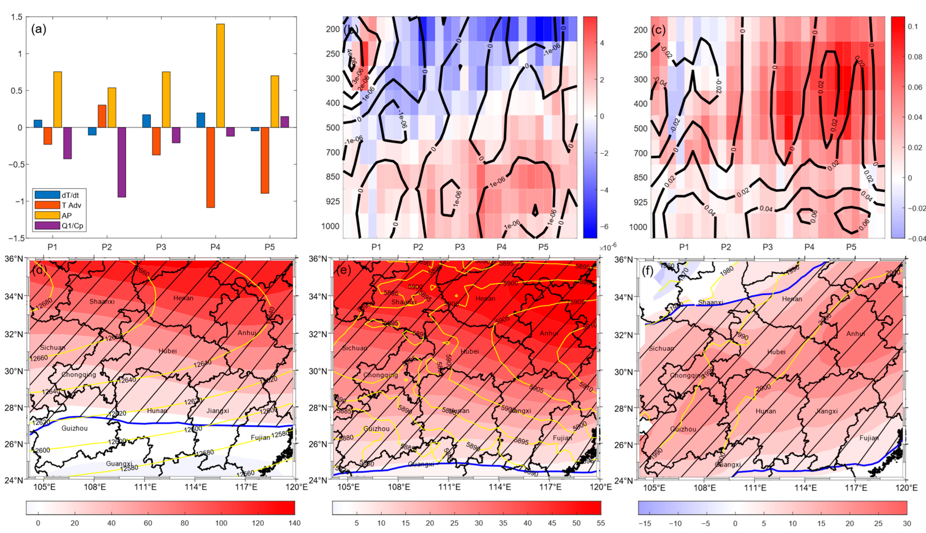
Figure 8.
(a) Temperature budget analysis results at 800 hPa in P1–6 over the MYRB. The four columns denote temperature tendency, horizontal advection of temperature, adiabatic heating related to vertical movement, and diabatic heating, respectively (K/day). (b) Temperature advection (shading; K/day) in P1–5 over South China.

Figure 9.
(a) Area average of South China in the control run (blue line; °C) and ERA5 reanalysis data (red line; °C). (b) Area average soil moisture (SMOIS) and MI30 in the control run (red line for SMOIS; m3 m−3, purple line for MI30) and ERA5 reanalysis data (blue line for SMOIS; m3 m−3, yellow line for MI30). (c,d) Average (shading; °C) and wind at 850 hPa (streamlines; m s−1) in the heatwave event in (c) the control run and (d) ERA5 reanalysis data.

Figure 10.
The decline in soil moisture (shading; m3 m−3) in P3–6 compared with P1 in the control run. The data have been subjected to a 3-by-3 kernel convolution.
Figure 10.
The decline in soil moisture (shading; m3 m−3) in P3–6 compared with P1 in the control run. The data have been subjected to a 3-by-3 kernel convolution.

Figure 11.
(a–c) Area average comparison between the control run (blue line; °C) and the sensitivity runs (red lines; °C). (d–f) The difference in average (shading; °C) in sensitivity runs compared with the control run. Slash hatches show that the area passed the 95% significance test.
Figure 11.
(a–c) Area average comparison between the control run (blue line; °C) and the sensitivity runs (red lines; °C). (d–f) The difference in average (shading; °C) in sensitivity runs compared with the control run. Slash hatches show that the area passed the 95% significance test.

Figure 12.
(a–c) Area average soil moisture (SMOIS) and MI30 comparison between the control run (blue line for MI30, yellow line for SMOIS; m3 m−3) and the sensitivity runs (red line for MI30, purple line for SMOIS; m3 m−3). (d–f) The decline in drought level in sensitivity runs compared with the control run (shading: orange block means one-level decline, brown block means two-level decline, and blue box means one-level increase).

Figure 13.
(a) The decline in temperature budget in the RMV-NSE run compared with the control run. The four columns denote temperature tendency, horizontal advection of temperature, adiabatic heating related to vertical movement, and diabatic heating, respectively (K/day). (b) The decline in divergence (shading; s−1) with the divergence in control run (black line, smoothened with 3-by-3 kernel convolution; s−1). (c) The decline in vertical speed (shading; Pa/s), with the black line showing the vertical speed in control run (smoothened with 3-by-3 kernel convolution; Pa s−1). (d–f) The decline in geopotential height (shading; gpm), with the yellow line showing the geopotential height in control run (smoothened with 3-by-3 kernel convolution; Pa/s) at (d) 200 hPa, (e) 500 hPa, and (f) 800 hPa. Slash hatches and blue lines denote areas that passed the 99% significant test.


Table 1.
Different MCIs and their corresponding drought level [28].
Table 1.
Different MCIs and their corresponding drought level [28].
| Level | Type | MCI |
|---|---|---|
| 1 | No drought | |
| 2 | Light drought (I) | |
| 3 | Moderate drought (II) | |
| 4 | Severe drought (III) | |
| 5 | Extreme drought (IV) |
Table 2.
Details of the PLF experiment.
| Control | RMV-N | RMV-SE | RMV-NSE | |
|---|---|---|---|---|
| Domain | 24°–36°N, 104°–120°E | 24°–36°N, 104°–120°E | 24°–36°N, 104°–120°E | 24°–36°N, 104°–120°E |
| ISO Removed | Unprocessed | Northern Boundary | Southern and Eastern Boundary | N, S, and E Boundary |
| Initial field | Original field generated from ERA5 data | Same as Control | Same as Control | Same as Control |
| Boundary field | Original field generated from ERA5 data | ISO removed from N Boundary | ISO removed from SE Boundary | ISO removed from NSE Boundary |
| Physical Parameterization | Refer to paragraph one of Section 2.2 | Same as Control | Same as Control | Same as Control |
Disclaimer/Publisher’s Note: The statements, opinions and data contained in all publications are solely those of the individual author(s) and contributor(s) and not of MDPI and/or the editor(s). MDPI and/or the editor(s) disclaim responsibility for any injury to people or property resulting from any ideas, methods, instructions or products referred to in the content. |
© 2023 by the authors. Licensee MDPI, Basel, Switzerland. This article is an open access article distributed under the terms and conditions of the Creative Commons Attribution (CC BY) license (https://creativecommons.org/licenses/by/4.0/).
Share and Cite
MDPI and ACS Style
Qin, Y.; Qin, Y.; Shen, Y.; Li, Y.; Xiang, B. Numerical Study on the Effects of Intraseasonal Oscillations for a Persistent Drought and Hot Event in South China Summer 2022. Remote Sens. 2023, 15, 892. https://doi.org/10.3390/rs15040892
AMA Style
Qin Y, Qin Y, Shen Y, Li Y, Xiang B. Numerical Study on the Effects of Intraseasonal Oscillations for a Persistent Drought and Hot Event in South China Summer 2022. Remote Sensing. 2023; 15(4):892. https://doi.org/10.3390/rs15040892
Chicago/Turabian StyleQin, Yi, Yujing Qin, Yichen Shen, Yonghua Li, and Bo Xiang. 2023. "Numerical Study on the Effects of Intraseasonal Oscillations for a Persistent Drought and Hot Event in South China Summer 2022" Remote Sensing 15, no. 4: 892. https://doi.org/10.3390/rs15040892
Note that from the first issue of 2016, this journal uses article numbers instead of page numbers. See further details here.