
High-Resolution Imaging of Radiation Brightness Temperature Obtained by Drone-Borne Microwave Radiometer


1
Northeast Institute of Geography and Agroecology, Chinese Academy of Sciences, Changchun 130102, China
2
University of Chinese Academy of Sciences, Beijing 100000, China
3
Jingyuetan Remote Sensing Experimental Station, Chinese Academy of Sciences, Changchun 130102, China
4
College of Geoexploration Science and Technology, Jilin University, Changchun 130026, China
*
Author to whom correspondence should be addressed.
Remote Sens. 2023, 15(3), 832; https://doi.org/10.3390/rs15030832
Submission received: 16 November 2022
/
Revised: 24 January 2023
/
Accepted: 30 January 2023
/
Published: 1 February 2023
(This article belongs to the Special Issue Microwave Remote Sensing for Quantitative Parameters Retrieval: Methods and Applications)
Abstract
:A digital automatic gain compensation (AGC) drone-borne K-band microwave radiometer with continuous high-speed acquisition and fast storage functions is designed and applied to obtain high-resolution radiation brightness temperature (TB) images. In this paper, the composition of the drone-borne passive microwave observation system is introduced, a data processing method considering the topography and angle correction is proposed, the error analysis of the projection process is carried out, and finally, a high-resolution microwave radiation TB image is obtained by a demonstration area experiment. The characteristics of the radiometer are tested by experiments, and the standard deviation of the TB is 1K. The data processing method proposed is verified using a demonstration case. The corrected data have a good correlation with the theoretical values, of which the R2 is 0.87. A high-resolution radiation TB image is obtained, and the results show the TB characteristics of different objects well. The boundary of the ground object is closer to the real value after correction.
1. Introduction
A microwave radiometer is a high-sensitivity broadband noise receiver working in a microwave band, which can extract the variation of a weak microwave radiation signal from strong background noise, and it mainly deals with the Gaussian white noise radiated from ground objects [1]. According to the carrying platform, it can be classified into spaceborne, airborne, or ground-based. The spatial resolution of the radiometer is determined by the beam angle of the antenna and the measurement distance [2]. In general, the spatial resolution of ground-based radiometers is the highest [3], and the data are distributed in points. The resolution of spaceborne radiometers is coarse [4,5], and the observed area is usually mixed pixels, which increases the uncertainty of inversion.
Traditional airborne passive microwave remote sensing complements the observation scale between spaceborne and ground-based remote sensing, enabling rapid and effective remote-sensing monitoring of designated areas and calibrating space remote-sensing detection data. Nevertheless, using manned aircraft is not cost-effective. The development of unmanned aerial vehicles (UAV) or drones in recent years has provided a new platform and way for remote sensing to monitor ground parameters at different temporal and spatial scales, which is difficult to do using traditional methods [6]. Table 1 compares the characteristics of manned aircraft and UAVs as carrying platforms.
Using a drone-borne microwave radiometer can realize the observation of the microwave radiation characteristics of specific targets in a region. It provides data at different scales, which fills the scale gap between ground-based remote-sensing experiments and space-based experiments. It can obtain high-resolution brightness temperature (TB) images of microwave radiation in real-time, which greatly reduces the acquisition cost of remote-sensing data, providing stable and credible TB data support at different scales for subsequent research. High-resolution microwave radiant TB images can provide good data support for the model inversion, establishment, verification, and ground verification of satellite data.
This paper introduces the composition of a drone-borne passive microwave observation system, proposes a data processing method considering the topography and angle correction, analyzes the error of the projection process, obtains a high-resolution microwave radiation TB image using a demonstration area experiment, and verifies the proposed data processing method.
2. Materials and Methods
2.1. Drone-Borne Passive Microwave Observation System
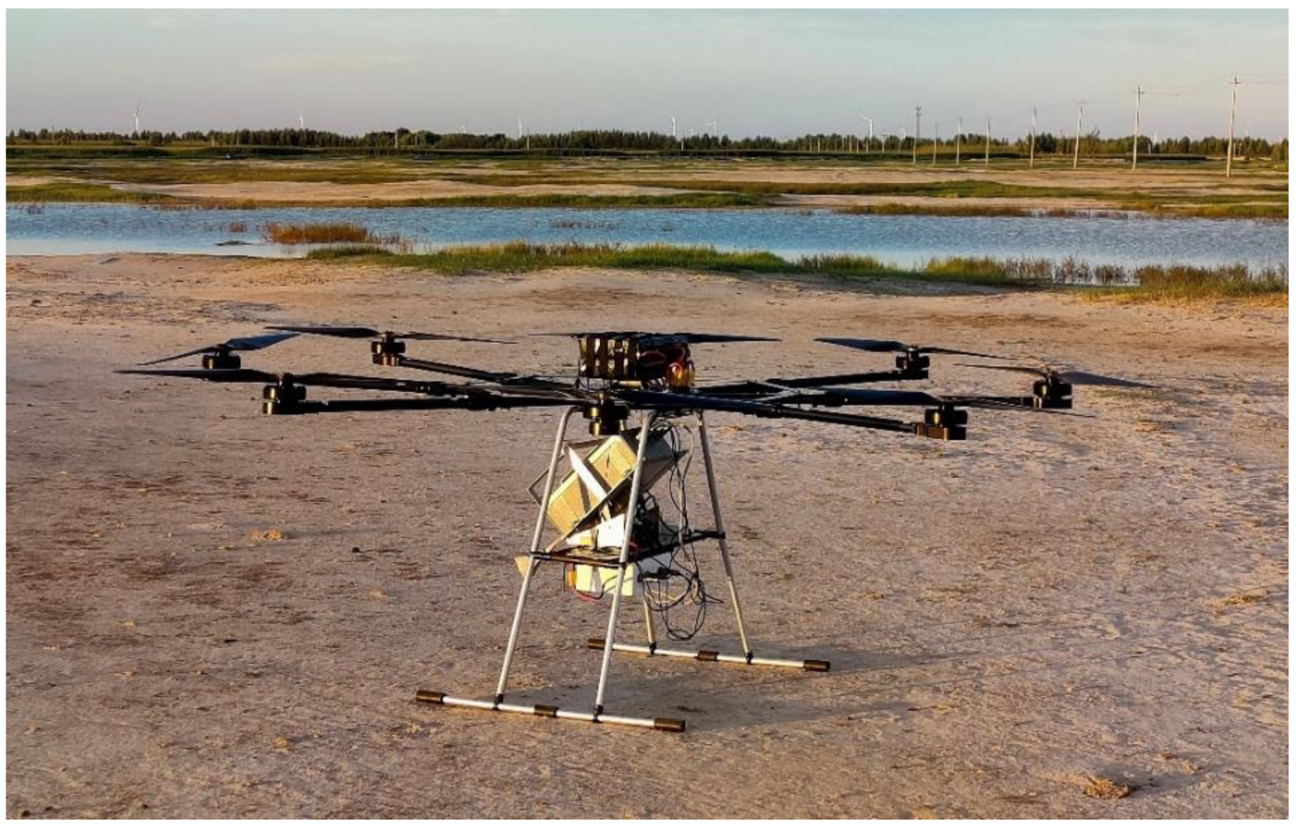
The drone-borne passive microwave observation system was mainly composed of a drone-borne microwave radiometer, flight attitude module, data transmission link, power supply system, ground command station, and flight platform, as shown in Figure 1.
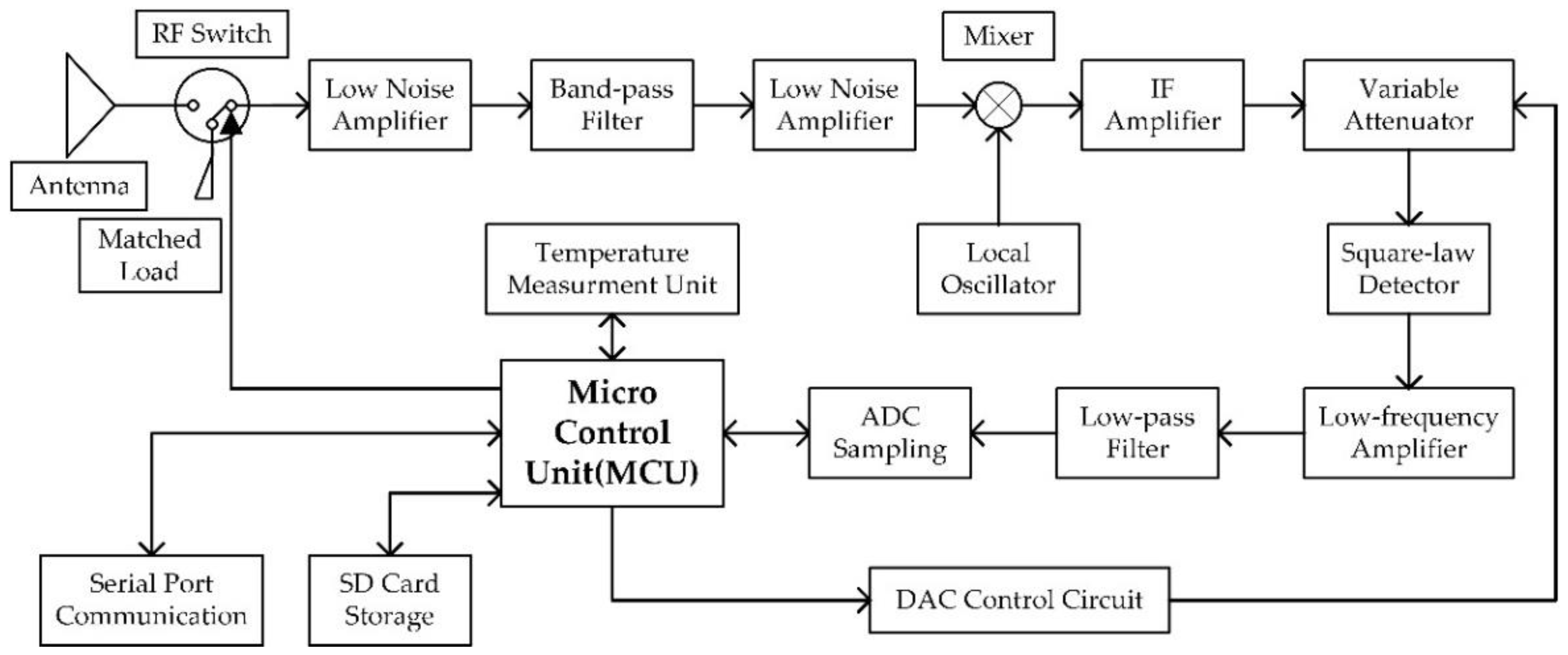
A K-band drone-borne microwave radiometer was used in this study. K-band is sensitive to moisture and is usually selected to study snow depth, snow water equivalent, lake freeze–thaw, and forest transmissivity models [7,8,9,10]. The radiometer was designed as a total power radiometer and adopted the digital automatic gain compensation (AGC) scheme [11,12], as shown in Figure 2. The RF switch periodically measured the antenna and reference source and corrected the antenna measurement value by measuring the gain variation of the reference source. It ensured the sensitivity and stability of the receiver, eliminated the complex hardware circuit feedback control link, and reduced power consumption. A standard gain horn antenna was used for the RF front end. The micro-control unit (MCU) of the traditional microwave radiometer was upgraded, and the ARM chip, with a small size and low power consumption, was adopted as the main control unit, which had the ability for fast acquisition and storage [13]. A multi-point temperature correction scheme was adopted to avoid the burden of weight, volume, and power consumption caused by the constant temperature system and ensured the working performance of the instrument. The receiver parameters are shown in Table 2.
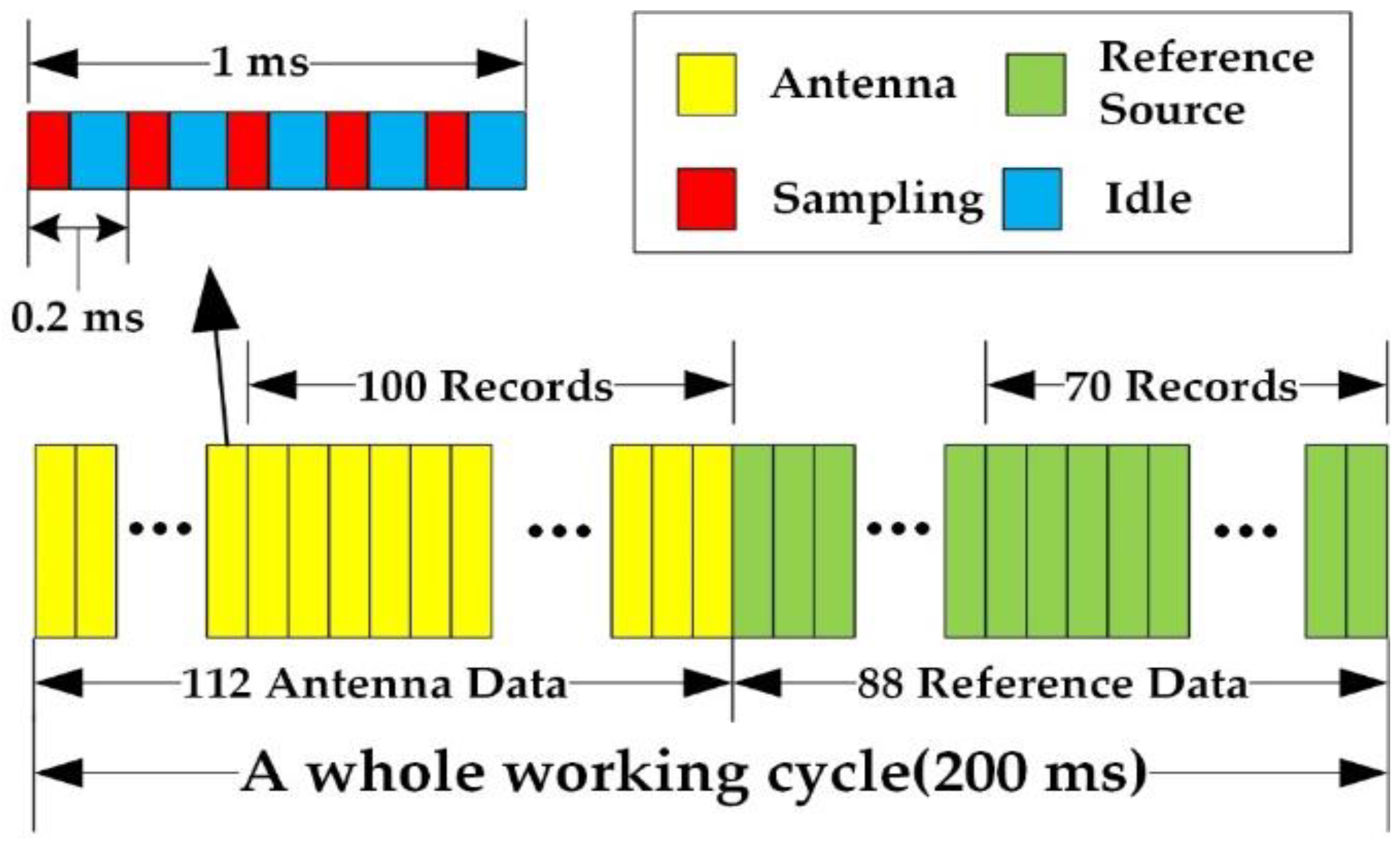
The working sequence of the radiometer is shown in Figure 3, and the integration time was designed to be 1 millisecond. According to the Nyquist sampling theorem, in order to completely retain the information of the original signal, the sampling period must be less than half, which was 0.5 milliseconds in this case, and thus it was set to 0.2 milliseconds. Each working cycle was 200 milliseconds, and the antenna and reference source were switched using the radio frequency switch, of which 112 were antennas and 88 were reference sources. After the RF switch was switched, the target needed a certain amount of time to stabilize. Therefore, we recorded the measured data of the last 100 antennas and 70 reference sources.
The flight attitude module provided the observation system with real-time attitude information and position information of the platform, mainly including the inertial measurement unit (IMU) and global positioning system unit (GPS). The IMU consists of a three-axis gyroscope, a three-axis accelerometer, a three-axis geomagnetic sensor, and a barometer [14]. The IMU measured the three-axis inclination, the speed of angle change, the direction of flight and heading, and the barometer calculated the current attitude.
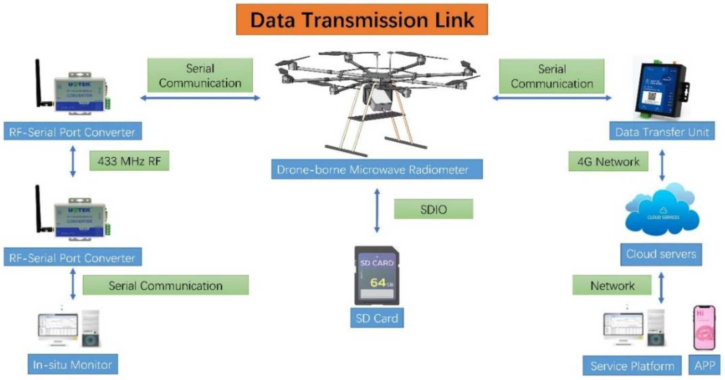
The drone-borne passive microwave remote-sensing observation system obtained the radiation TB of ground objects in a small area. The microwave radiometer was responsible for collecting TB information, and the GPS provided flight information, including the longitude and latitude, altitude, heading, speed, etc. Finally, the acquired information was summarized into the microwave radiometer for real-time matching, processing, and coding. All the original data would be stored in the secure digital (SD) card using high-speed data storage technology [13], and part of the main information would be extracted and sent to the ground command station through the wireless link for real-time viewing. The data transmission link is shown in Figure 4.
The drone-borne passive microwave observation system used a DC 24V battery to supply power to different equipment by converting the corresponding voltage through the DCDC power module. Inductance was added among the devices to isolate the ground so that there was no electrical interference, and electromagnetic compatibility was achieved.
The ground command station was responsible for controlling the flight operations, in situ real-time data monitoring, cloud monitoring, and real-time data processing, and had the ability of on-site rapid data processing and imaging. In addition, the research design used a separate set of transmission links instead of UAV flight control for the data transmission so that the system could be transplanted to any aircraft platform. The system itself formed a closed loop, which increased its portability.
2.2. Data Processing Method
The original data collected by the drone-borne passive microwave observation system mainly included three categories: (1) the TB of the target object measured by the antenna—the measured signal was mixed, amplified, and AD sampled after detection. The electrical signal was connected to the MCU through the serial peripheral interface (SPI); (2) the temperature of the matching load and each internal device was measured by sensors—the electrical signal was also connected to the MCU through the SPI interface; (3) the flight attitude information obtained by GPS and other modules—the measured signal was sent to MCU through the serial port after level conversion.
In addition, the data also contained the time sequence number, the data frame number, and other information. All data were stored in an SD card after preprocessing and coding. After the flight, the data stored on the SD card were decoded using the card reader and sent to the computer through the serial port for processing.
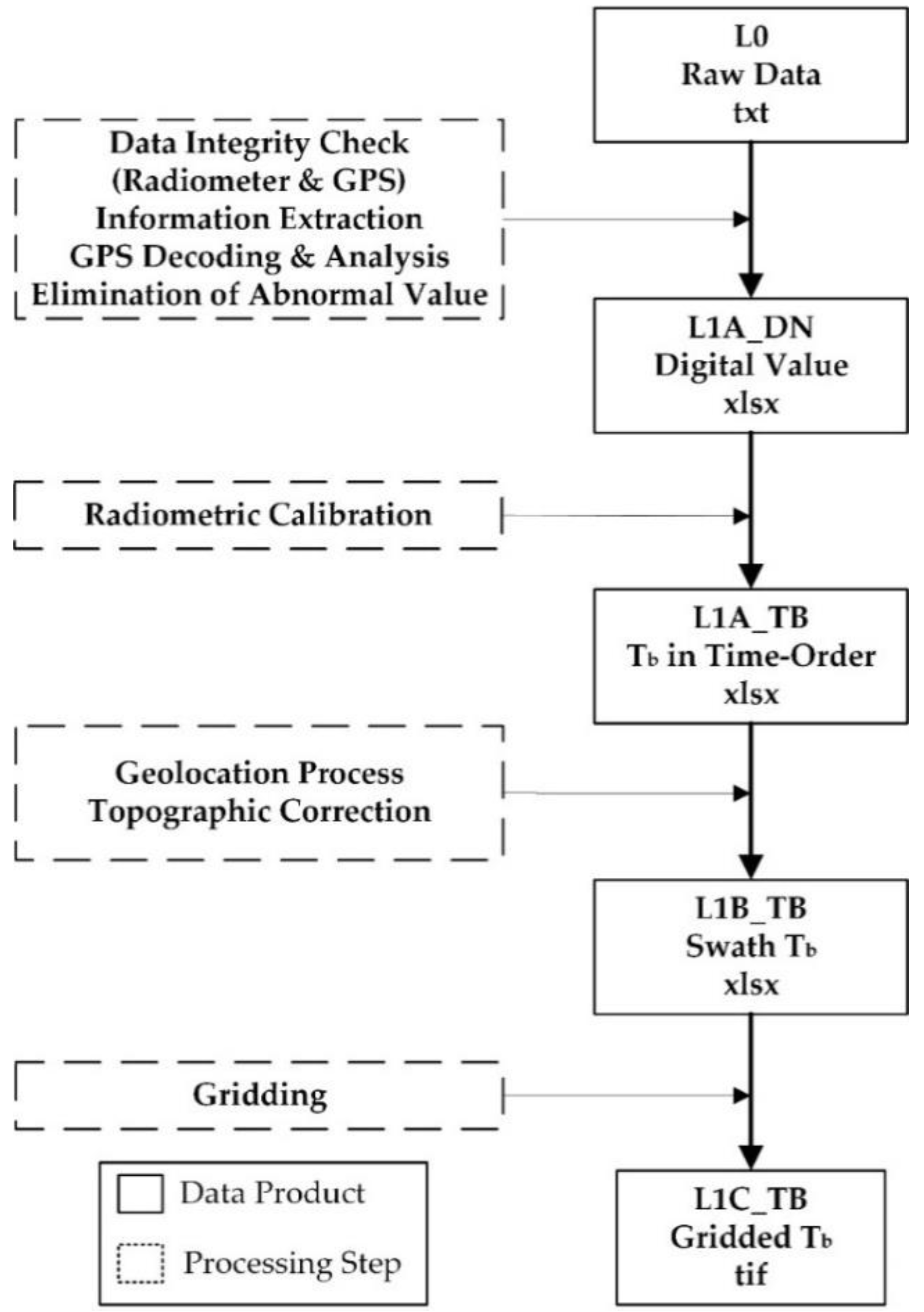
A data-processing method of a microwave radiometer carried by a UAV is proposed. This study refers to the operation and naming methods of satellite data products for all levels of data, as shown in Table 3. The raw data obtained were defined as L0 data, and the data were recorded in ASCII code.
After the raw data extraction, interference detection, radiometric calibration, and geolocation process, the L0 data could be obtained in the L1B swath data in time order, and L1C gridded data could be obtained after the grid transformation. The data processing flow is shown in Figure 5. The data processing method included 6 processes: (1) data extraction, (2) data selection, (3) radiometric calibration, (4) GPS interpolation, (5) data space projection, and (6) gridding and generating a preview map of TB spatial distribution. The functions and methods of each process are described in detail below.
2.2.1. Data Extraction
The main purpose of the data extraction process was to analyze the original data according to the preset encoding method to obtain useful information. The L0 data were the original data stored by the radiometer. After the data integrity inspection, checksum secondary verification, field extraction, GPS analysis, and removal of outliers, the digital value of the time-order L1A_DN data was obtained.
The results were generated into Excel tables. The extracted information included the following information: data serial number, gain compensation, antenna average digital value, reference source average digital value, date, time, longitude, latitude, radiometer direction, elevation, temperature, antenna original digital value, and reference source original digital value. The temperature data were used in the multi-point temperature correction algorithm, and the original antenna and reference source data were in millisecond integration time.
2.2.2. Data Selection
After the data extraction, all the original data were extracted and stored in the form of tables, including a lot of unnecessary information, such as the non-flight operation period, takeoff and landing period, reciprocating survey areas and turns, etc. These data were redundant and did not affect the processing results. They were removed before the other steps to save computing power and resources.
The main basis for the selection was to reproduce the flight path according to the longitude and latitude, heading angle, and elevation information of the time series obtained in the previous step to select an appropriate time period. Meanwhile, considering that the actual flight operation was affected by airflow, the flight attitude also differed in different flight directions, which would affect the modeling results. Therefore, it was very necessary to intercept and classify the data at different time periods.
2.2.3. Radiometric Calibration
The data measured by the microwave radiometer were digital values, and thus the TB values needed to be obtained after calibration. The calibration of the drone-borne microwave radiometer included receiver calibration and overall calibration.
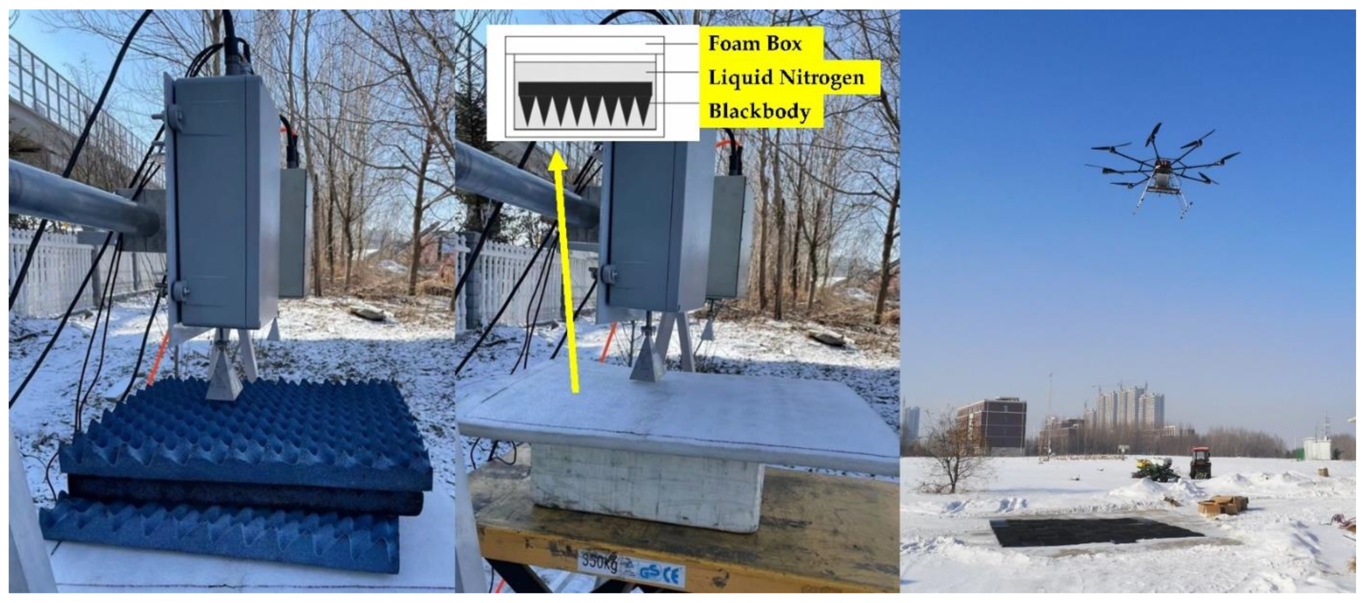
The calibration equation of the receiver could use the two-point calibration method [15] since the linearity of the microwave radiometer receiver was good. A two-point calibration method was used to measure the liquid nitrogen and blackbody, obtain two sets of output voltage, and establish the relationship with the brightness temperature. The experimental photos are shown in Figure 6.
According to Planck’s blackbody radiation law, the physical temperature of the blackbody must be equal to the ambient temperature for it to absorb all external electromagnetic radiation. Then, we have
where the subscripts BB and LN represent blackbody and liquid nitrogen, respectively.
The boiling point of liquid nitrogen at standard atmospheric pressure TLN was 77K. The physical temperature of the blackbody measured by the thermometer was 254.3K during the calibration experiment. The digital values from the radiometer were 929 and 2533, respectively. Substituting these conditions into Equation (1), the expression in the form of Equation (2) could be obtained, which was the calibration equation of the radiometer receiver.
The overall calibration was obtained by experimental measurement. A certain area of the blackbody was placed on the ground, and the UAV carried a radiometer to measure the blackbody continuously for a period of time in flight. The experimental photos are shown in Figure 6 (right).
Under the condition of a flying altitude of 5 m, an observation angle of 50°, and a half-beam angle of 7.5°, the instantaneous field of view of the radiometer was an ellipse of 3.3 m × 2.1 m. In order to minimize the influence of side lobes, a blackbody of approximately 7 m × 5 m was laid on the ground for the experiment.
The real-time temperatures of the main components inside the radiometer or the amplifier circuit were measured by applying the multi-point temperature correction scheme to minimize the negative impact caused by temperature drift.
After obtaining the calibration equation of the microwave radiometer, the digital values of the L1A_DN data were radiometrically calibrated, and the TB values of the L1A_TB data were obtained in time order.
2.2.4. GPS Interpolation
Since the radiation TB sampling frequency was higher than the GPS sampling frequency, it was necessary to interpolate the matched GPS data with equal spacing (linear interpolation). In most cases, the speed of the UAV platform was relatively stable during flight, and the geographic information obtained by GPS was continuous in the time domain. According to this feature, we were able to perform linear interpolation on the GPS data.
The radiometer sampling interval was T1, and the GPS sampling interval was T2. We had to linearly interpolate n = T1/T2-1 points in the adjacent GPS sampling points to spatially match the corresponding TB data. The longitude and latitude of the two adjacent GPS sampling points were Lon0, Lat0, Lonn+1, and Latn+1, and the longitude and latitude of the interpolation points were
where i = 1, 2, 3…n.
In addition, if the radiometer failed to sample once during the period and did not store it, the frame number was used to determine the location of the actual data and make corresponding corrections.
2.2.5. Data Space Projection
Space projection usually refers to the geolocation process and topographic correction. When applying a series of data processing operations, L1A_TB data were obtained, which included position and attitude information of the radiometer and the measured TB. Then, the flight attitude modeling and projection could be carried out to obtain the geographic position corresponding to the center beam and its field of view (FOV). The observations of the planar terrain and complex terrain were modeled, and the radiometer TB swath data L1B were obtained after the space projection.
The Functional Equation of the Main Beam and the FOV
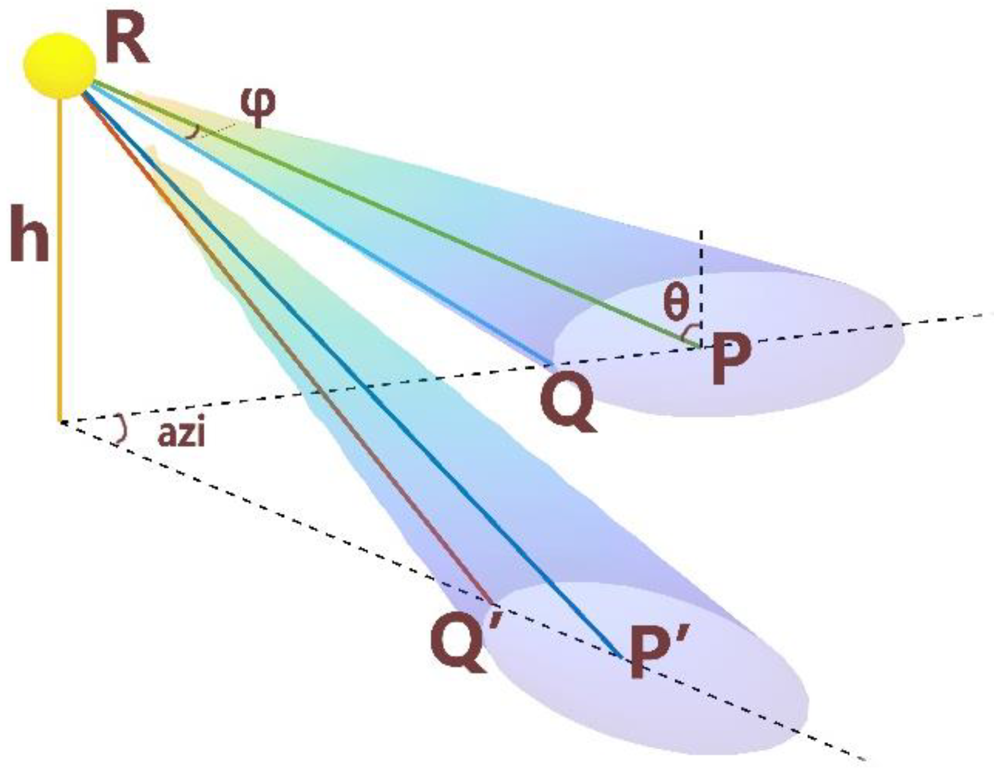
Considering only the energy radiation in the beam angle range, the effective FOV received by the antenna could be simplified as a conical oblique incident on a plane, resulting in an ellipse. The coordinate system was established according to the UAV attitude and the geometric relationship of the radiometer FOV, as shown in Figure 7.
Point R(x0,y0,h) is where the radiometer was located. The incidence angle was θ, the azimuth angle was azi, the half-beam angle was φ, and the flight height was h. Then, we obtained the equation of the rotation surface (for mathematical proofs, see Appendix A):
where
in accordance with
The field boundary of the radiometer could be obtained using the general form of the functional Equation (4) in conjunction with the plane equation. Taking azi = 0 as an example, the FOV of the radiometer could be expressed as
Center Beam Projection of Drone-Borne Microwave Radiometer
Similarly, we were able to calculate the projection point of the radiometer’s center beam by distance and direction. Given the longitude, latitude, and altitude of the radiometer, the longitude and latitude of the projection point could be calculated based on its geometric relationship. We obtained
where the subscripts ‘pro’ and ‘UAV’ represent the projection point and UAV platform, respectively; Lon and Lat represent the longitude and latitude, respectively; the subscript ‘co’ is the conversion coefficient of the actual distance (in meters) corresponding to the projection coordinate system (in degrees) during the projection process.
For every degree in latitude along the longitude line, the actual distance was approximately 111 km. Along the latitude line, the actual distance was 111 × cos (Lat) kilometers for each degree in longitude. Taking the latitude of the experimental area in this study at approximately 44°N as an example, we obtained
Influence from Terrain Slope and Aspect
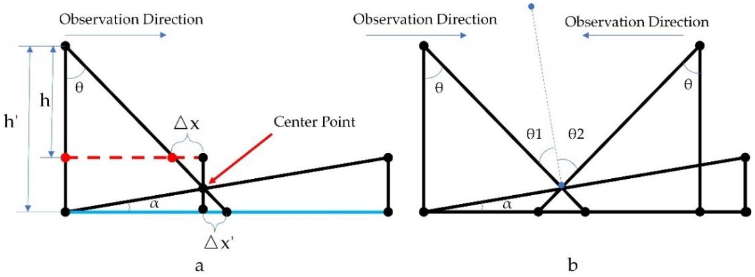
When the observation target was not flat or complex, the relief and slope of the terrain led to the offset of the actual projection point and the change of the incidence angle. The side view of its observation direction profile is shown in Figure 8.
In Figure 7a, the observation angle of the radiometer is θ, the slope angle is α, and the vertical distances between the UAV platform and the slope top/bottom are h and h′. When the UAV took off from the plane at the top of the slope (as shown in red), the actual measured center point was closer than the calculated projection point in the flight direction, as shown in △x in Figure 7a. Correspondingly, it would be farther than that when taking off at the bottom (as shown in blue) by △x′. Certainly, the actual takeoff position could be any altitude, and thus the digital surface model (DSM) of the actual measurement area had to be determined.
As for the issue of incident angle correction, a brief schematic diagram is provided in Figure 7b. When the slope aspect and the flight direction were along the same line, the original incident angle θ changed, which was related to the angle between the slope aspect and the flight direction (0 or 180°); that is, along the slope or against the slope. According to the geometric relationship, the corrected incidence angles were θ±α. The TB of the object changed with the change in incident angle, so it would have a certain impact on the final result.
In practice, the observation incidence angle was not only related to the slope and observation zenith angle, but we also had to consider the observation azimuth and aspect angle. In this study, the incident angle of the drone-borne microwave radiometer was corrected through modeling and applied to the subsequent modeling.
The change in the actual terrain affected the projection results, which was mainly reflected by the partial position shifting and stretching in the image. Due to the spatial heterogeneity of the terrain and the undulation of the ground, and considering the practical application, there were many methods to determine the projection point of the main beam on the ground, and the solution process required balancing accuracy and computation.
The Projection Process
The projection process considering the actual terrain and the modeling process are discussed below.
- (1)
- Resampling the DSM and establishing the coordinate system
The DSM obtained had a high spatial resolution, so it was resampled to save computational resources. The longitude, latitude, and altitude of the coordinate origin were selected, and all data were converted into meters to unify the units. Note that the selection of the coordinate origin should not pass through the terrain, which would simplify the subsequent calculation.
- (2)
- Analytic linear equation of the main beam
The position of the UAV platform was P(x1,y1,z1), the observation azimuth was m, and the observation incident angle was n. Then, the linear equation of the main beam l was
and the direction vector was s = (sin m,cos m,−tan−1 n). Given any one of the parameters in x, y, and z, the other two parameters can be obtained.
- (3)
- Finding the intersection point of the main beam and the observation surface
There were many methods to determine the intersection point between the main beam and the observation surface. Considering that the number of points on the main beam ray was far less than that on the observation surface, we compared the methods and finally designed a method with a minimal computational cost.
By making the point U (x4,y4,z4) on the beam center step in the direction vector s, the distance between the U and the DSM discrete points directly below was found and calculated. The minimum distance corresponded to the projection point. When the step size was small enough, we could obtain a relatively accurate intersection point, but that would greatly increase the calculation amount. Therefore, we chose to divide the step into large sections first by hierarchical steps and then divided those steps into small sections after roughly searching the range, which greatly reduces the computational load.
The negative half-axis of the z-axis t = (0,0,−1) was chosen as the stepping direction ( the reasons are explained in Appendix B). The calculation steps were as follows:
(a) z4 was traversed between z1 and z1 − k1 × 50 according to the large step = k1, and the b~c operation was performed for each z4;
(b) The corresponding x4 and y4 were calculated according to Equation (8);
(c) The z2 corresponding to the point (x2,y2) was found, which was the closest to (x4,y4) in the DEM discrete point, and |z4 − z2| was calculated;
(d) The minimum value of all |z4 − z2| was found and located, and the corresponding z4 was marked as zmin;
(e) z4 was traversed between zmin − k2 × 3 and zmin + k2 × 3 according to the object step = k2 (where k2 was the final search precision);
(f) The b~d operation was repeated and the intersection position U (x4,y4,z4) was obtained within the final accuracy of k2 deviation;
- (4)
- The partial slope functional equation was established to calculate the slope and aspect.
The points within a certain range were searched near the projection point, and the partial slope functional equation was established and expressed as
(the mathematical calculation process is shown in Appendix C) and the slope α and aspect β could be calculated by
- (5)
- Incidence angle correction
The incidence angle was corrected by Equation (11) (the mathematical proofs can be found in Appendix D), and the change of the FOV was temporarily ignored.
where the observed zenith angle is , the azimuth angle is , the slope angle is , and the slope aspect is .
2.2.6. Gridding
A key part of passive microwave radiation TB image processing is to convert swath-based measurement data into grid data. There are many methods and algorithms for this, for example, resampling or interpolation and image restoration or reconstruction techniques. The algorithms were selected considering the balance of noise and spatial resolution. Classical drop-in-the-bucket (DIB) techniques provide low-noise and low-resolution products while using image reconstruction techniques provides higher-resolution (and possibly higher-noise) products [16,17].
DIB averaging is a classical coarse-resolution meshing process. The center of each measurement location is mapped to an output projection grid cell. All measurements whose centers fall within the boundaries are added to the average, and the unweighted average becomes the reported pixel value.
2.3. Error Analysis of Geolocation Process
Due to the influence of the instrument sampling rate and sampling accuracy, there might be some errors in the collected data, which would have a certain impact on the accuracy of the geolocation process. As mentioned above, the projection point of the center beam (Pospro), the range of FOV (RangeFOV), the corrected incidence angle (Incicor), and the corrected azimuth angle (Azicor) were functions of the current position and orientation of the UAV platform and radiometer attitude and terrain, which can be expressed as
The descriptions and expression forms are shown in Table 4.
The corrected azimuth angle was determined by the yaw angle of the UAV and the planned heading. The corrected incidence angle was determined by the observation angle of the antenna during installation and the pitch angle of the UAV. The two corrected angles were used to correct the final incidence angle together with the slope and aspect, as mentioned above. The position information of the error was affected by the measurement accuracy of the GPS device, and there was static and dynamic drift during the measurement, which might have led to an error of 0~6 m, which we were not able to correct temporarily. The attitude information of the error was provided by the IMU, which might also have had several degrees of error due to its own sampling frequency and sampling accuracy limitations.
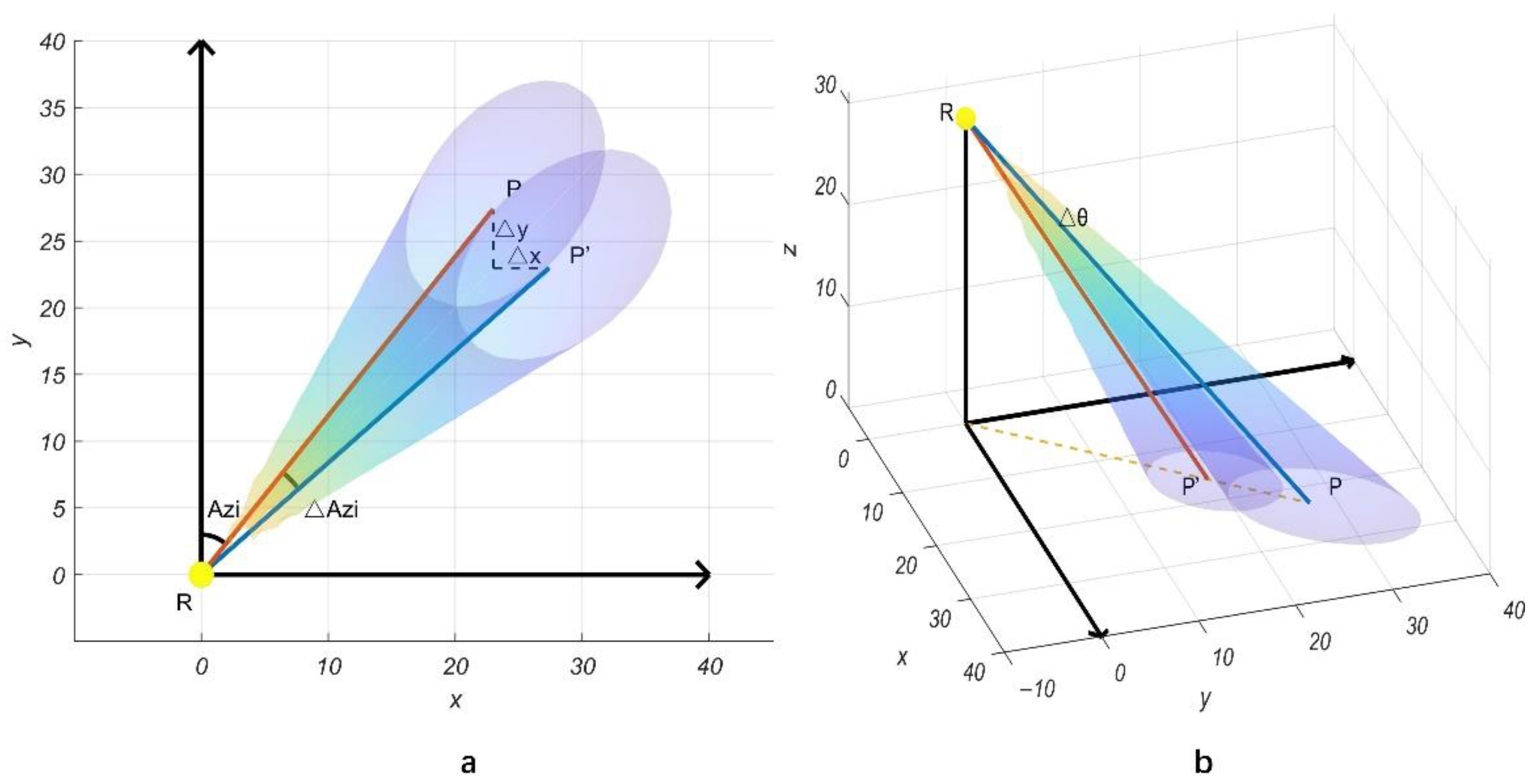
Due to the influence of airflow, the UAV had to adjust its flight attitude all the time during the flight operation, which led to the constant change in the observation azimuth and incident angle. The change in the observation azimuth angle only changed the position of the projection point, and the shape of the FOV remained unchanged, while the change in the incident angle changed both the position of the projection point and the shape of the FOV, as shown in Figure 9.
The expressions of the calculated changes or offsets were provided in the previous part of the paper. For a more intuitive display, the following took a flight altitude of 30 m, an incidence angle of 50°, an azimuth angle of 40°, and a half beam angle of 7.5° as examples to show the influence of small variation on the projection point and the FOV, as shown in Table 5.
3. Experiments, Results, and Discussion
3.1. Radiometer Characterization
3.1.1. Ground-Based Test of Dynamic Range and Stability of Microwave Radiometer
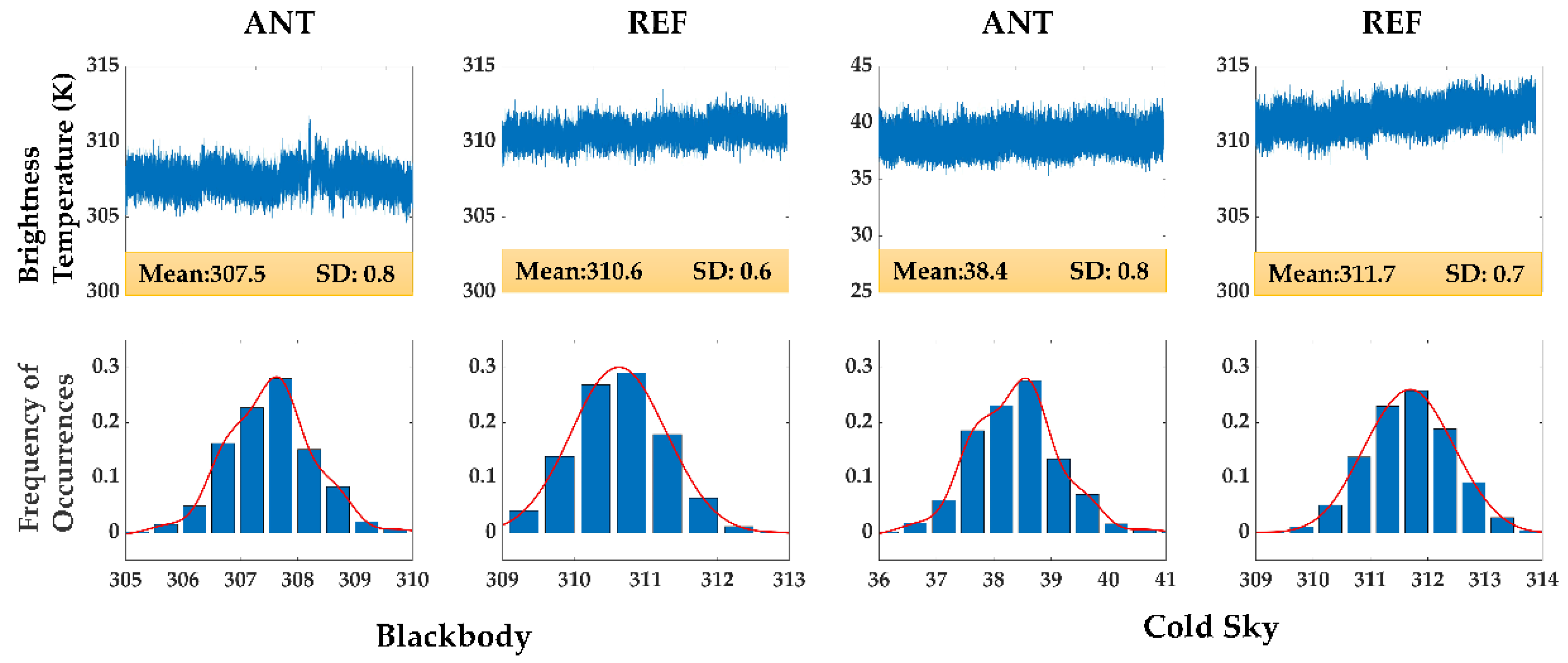
The stability and dynamic range of the K-band microwave radiometer carried by the UAV were tested. The microwave radiometer measured the black body and cold air for a long time and observed the TB of the antenna and the reference source. The experimental results of the K-band radiometer are shown in Figure 10. The average TB values of the blackbody and the cold air measured by the antenna were 307.5K and 38.4K, respectively, which show a good dynamic range and reflect the TB characteristics of the target. During a period of measurement, the standard deviation of the antenna and the matched load TB time series was basically kept in a small range, which was 0.8K, 0.6K, 0.8K, and 0.7K, indicating good stability of the device.
3.1.2. Flight Test of Drone-Borne Radiometer Dynamic Range and Stability
In order to determine if the UAV flight would affect the performance of the radiometer, we designed a set of experiments to determine whether the radiometer receiver was stable by comparing the TB of the matched load when the UAV rotor was working and at rest. Different objects were measured during flight, which reflected the radiation TB properties of different ground objects and verified the detection performance of the drone-borne microwave radiometer.
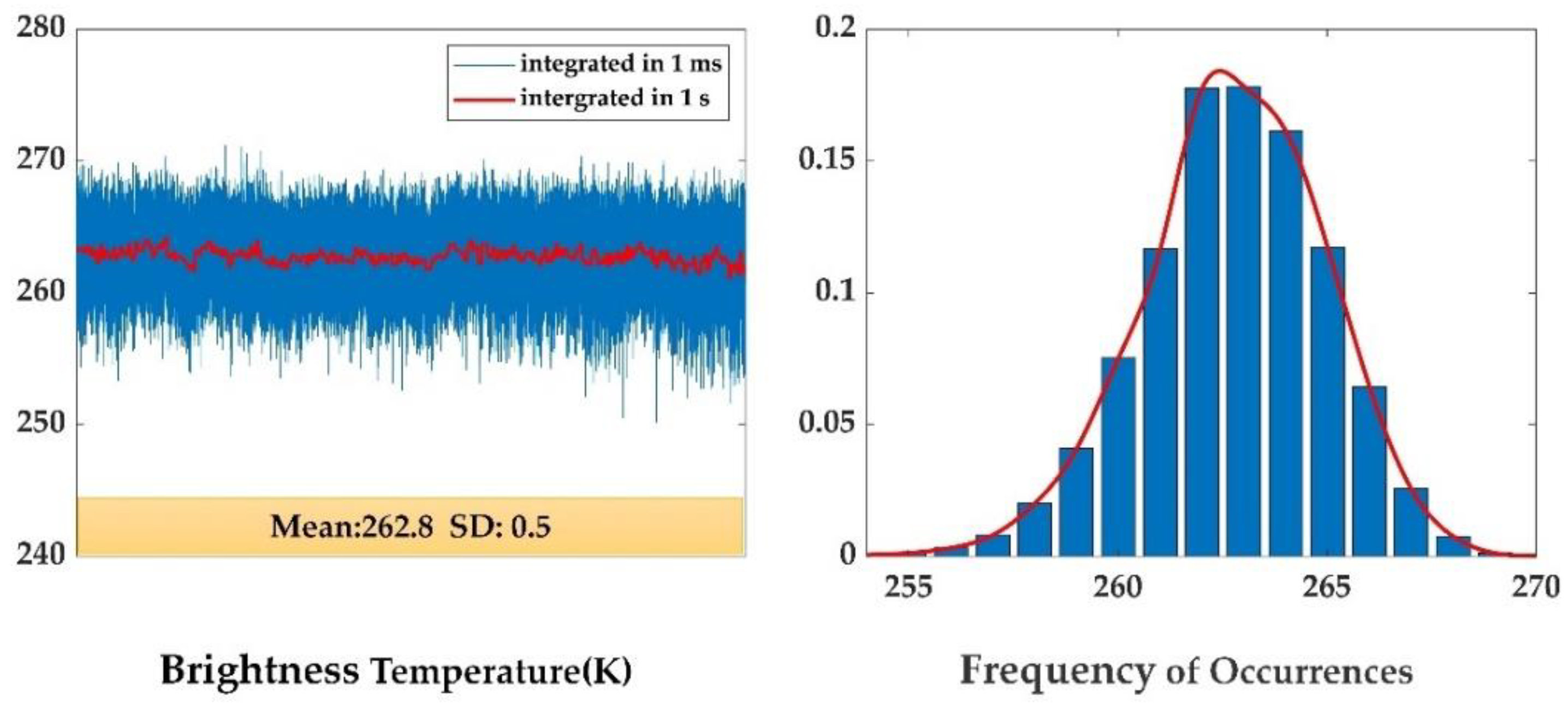
(1) The matching load was connected to the antenna. The TB time series of the matched load was monitored and integrated in milliseconds when the UAV was in the working state. The standard deviation was calculated to determine whether the stability performance of the radiometer was affected by the working state of the UAV platform. The results are shown in Figure 11.
The stability of the radiometer during the UAV rotor rotation was almost the same as when stationary on the ground. The average TB was 262.8K, and the standard deviation of the TB obtained was 0.5K in 1 s integration time. The results show that when the UAV was working, the electromagnetic interference coupled with the high-speed rotating rotor coil and the influence of the internal vibration caused by an uneven rotor speed hardly had an impact on the radiometer, which met the design requirements.
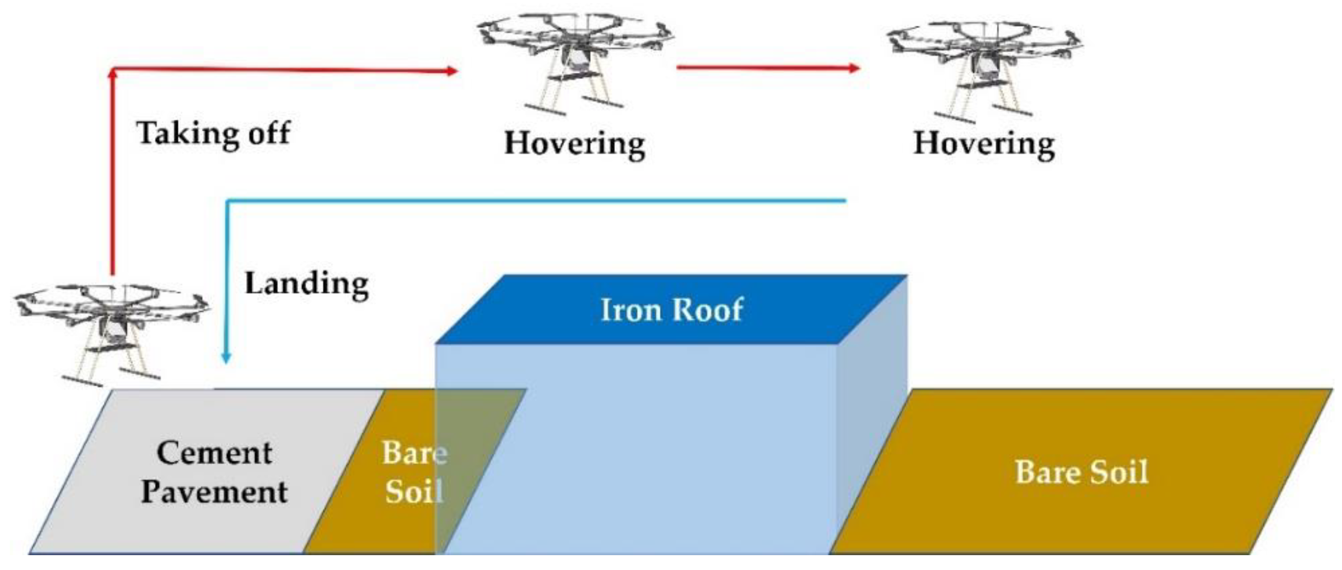
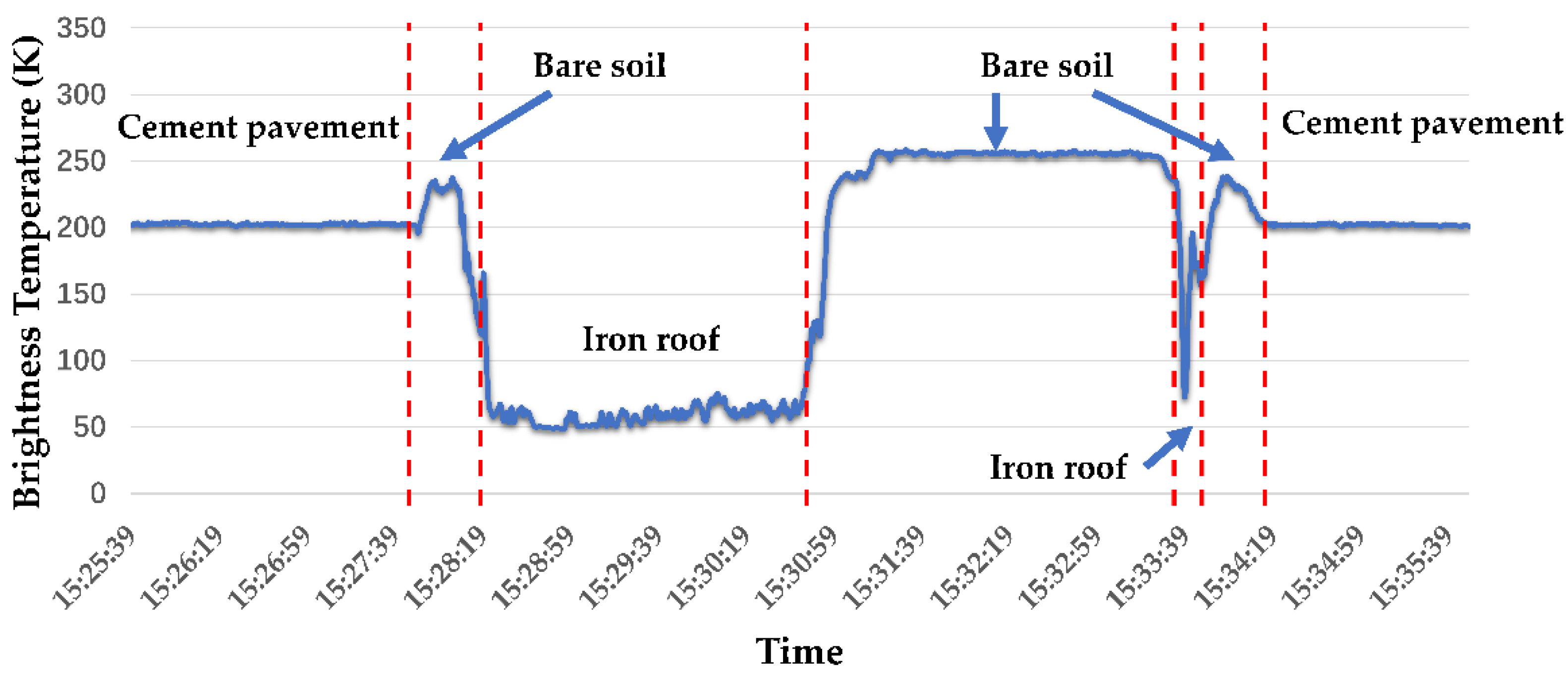
(2) The experiment was conducted in winter. The experimental design flew over an iron roof (reflecting the cold sky), bare soil on farmland, and cement pavement. When reaching the specified measurement target, the UAV hovered for a period of time. The schematic diagram of the flight path is shown in Figure 12. The UAV took off from the cement pavement, illuminated a small section of bare soil during its ascent, illuminated the iron roof (reflecting the cold sky) for a period of time, flew above the bare soil for a period of time, returned, and landed, during which it passed over the iron roof and bare soil again.
The measured TB results are shown in Figure 13. The TB values of the cement pavement, bare soil area, and iron roof were approximately 200K, 250K, and 60K, respectively. The results show that the drone-borne radiometer reflected the TB characteristics of different ground objects as well as the ground measurement.
The drone-borne passive microwave remote-sensing observation system could provide the TB of different targets within a certain area of pure pixels (depending on the FOV and the area of the target) and could also observe the gradual change process of the TB of the mixed pixels between the transition strips of the ground objects. It had a great improvement in spatial resolution compared to the spaceborne and airborne passive remote-sensing methods and a great improvement in mobile convenience compared to ground-based measurement.
3.2. Flight Experiment with Complex Terrain Observation Target
In order to verify the proposed spatial projection method of complex topographic data, we selected a small lake surrounded by bare soil on the campus of the Northeast Institute of Geography and Agroecology, Chinese Academy of Sciences located in Changchun, Jilin Province, China, as the experimental area. The experiment was carried out in winter when the lake was frozen, and there was 1~3 cm of snow (microwave can penetrate thin snow, so it had no effect on the experiment). The elevation of the lake was 194 m, the lowest in the region, and its edge gradually rose to 200 m. The experimental area was a rectangle of 270 m × 80 m. A total of five routes were designed, of which three flew west, and two flew east, with azimuths of 270° and 90°, respectively, and an incident angle of 55° for ground observation. The route length was about 210 m, and the route spacing was about 15 m.
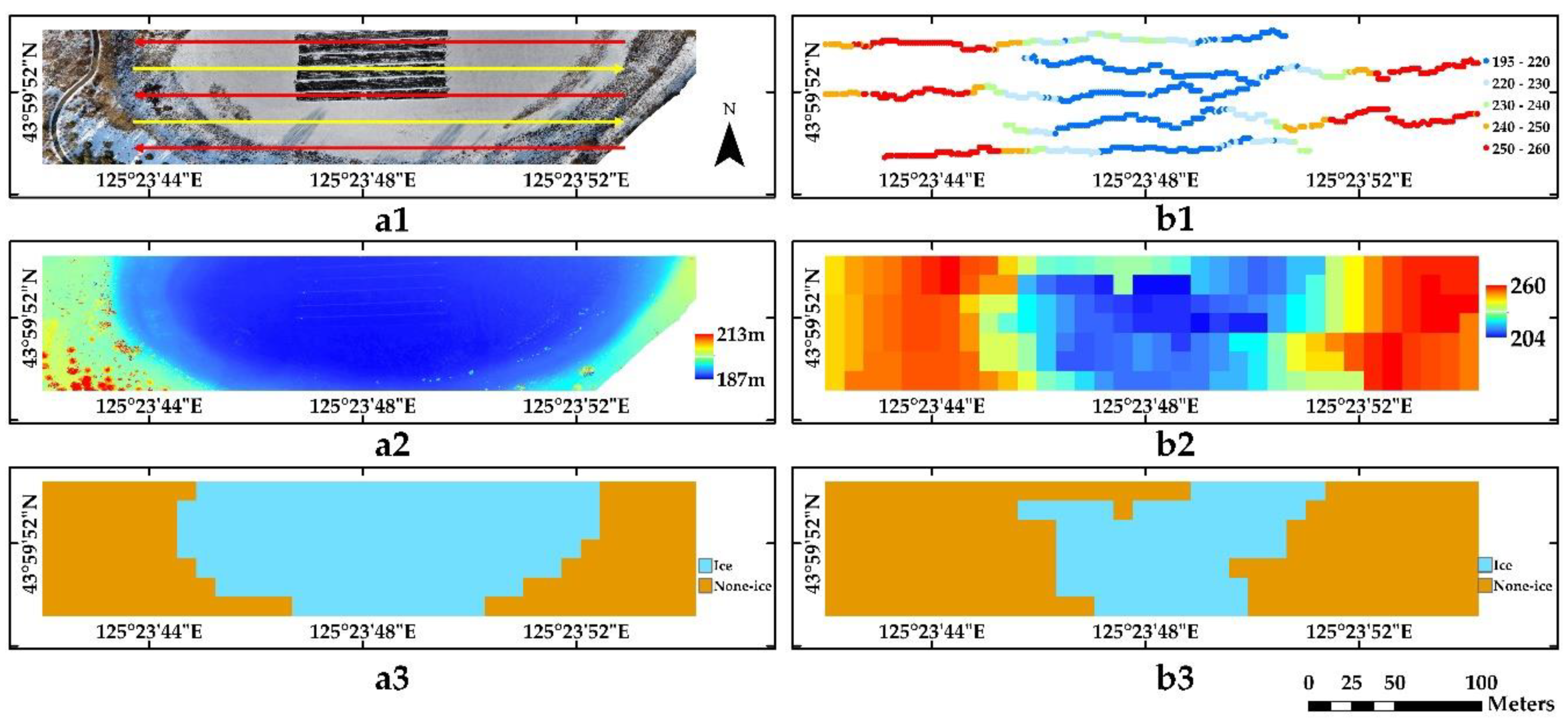
The experimental results are shown in Figure 14; Figure 14a1–a3 shows the optical image and the flying routes, the digital surface model (DSM) data, and the ground object classification results of the study area, respectively. Using the data processing method in Section 2.2, the TB swath data and the TB gridded data (resampling spatial resolution of 0.0001°) in the test area were obtained, as shown in Figure 14b1–b2. The results show that the TB of the ice surface was relatively low, ranging from 195–215K, while that of the bare soil area was relatively high, exceeding 250K, and the middle area was a transition strip. The system could accurately measure the TB of different ground objects and provide the value of pure pixels.
A threshold of 220K was selected to classify the lake ice area and non-lake ice area, and the binarized raster data are shown in Figure 14b3. Compared to the classification results of the optical image, the ice surface range identified by microwave was relatively small, which might have been caused by the following: (1) the selection of the threshold value would have affected the classification results. The pure lake ice pixels were selected, and the mixed pixels within transition bands were not included. (2) The ice thickness at the edge of the lake was relatively small, and the microwave could penetrate it to a certain degree, so the bare soil under the ice was detected. The classification results could roughly distinguish the boundary and were in good agreement with the actual boundary shape.
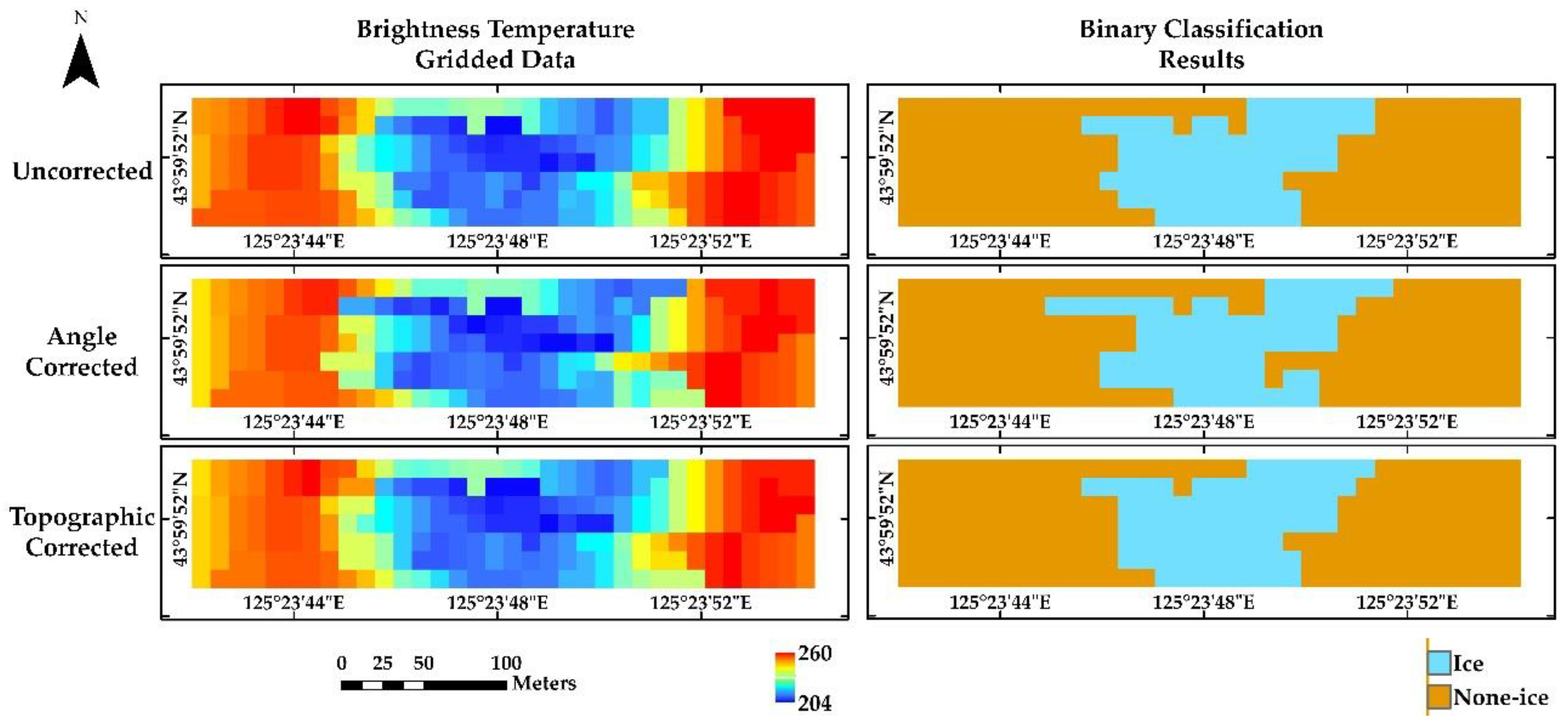
Meanwhile, the performances of the same set of original data for uncorrected, angle-corrected, and terrain-corrected data were compared to verify the proposed algorithm and method. The TB gridded data and binary classification results are shown in Figure 15. The results show that, after the angle correction, the position of the projection point was obviously offset, which led to an obvious ‘in–out’ phenomenon of the lake ice area in the image, and this phenomenon significantly improved after the topographic correction.
Compared to the ground-based measurement, the incidence angle would be changed by the flight attitude of the UAV, which would affect the projection position of the beam center and the range of the FOV. The incidence angle on the ground was 55° and 50° after the modification of the UAV attitude. When the flight altitude was 30 m, the central projection point needed to be corrected 7 m backward along the observation direction. On this basis, since the altitude of the survey area was lower than the takeoff altitude, according to the previous analysis, the central projection point needed to be corrected forward along the observation direction, and the amount of correction depended on the altitude difference between the survey area and the takeoff position.
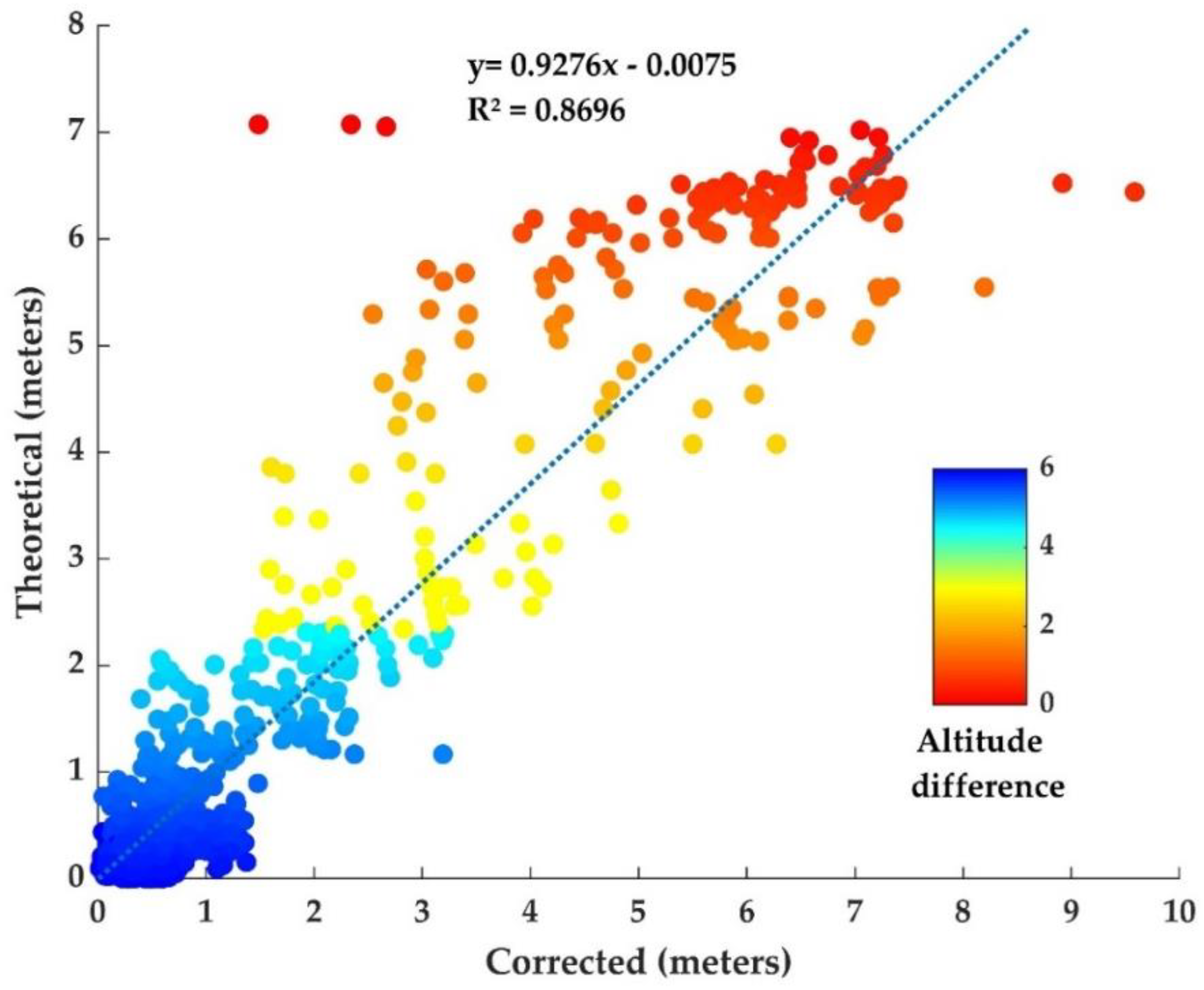
The corrected offsets, or the distances between the uncorrected points and corrected points using the data processing method proposed in sub-section “The Projection Process”, were measured, and the altitudes of the projection points were extracted. Then, the theoretical quantities of the offsets could be calculated using the altitude differences with
where h and h′ are the flying height and altitude difference, respectively, and θ and θ′ are the observation angle before and after correction, respectively. The theoretical quantities and corrected offsets of the proposed method were compared, and the result is shown in Figure 16. The altitude difference between the measurement target and the takeoff position is shown in different colors. The calculated theoretical value and the corrected value based on the actual angle and terrain were very close to the 1:1 line, and the R2 was 0.87, which verifies the effectiveness of the angle and terrain correction method proposed.
Interestingly, there was a certain degree of similarity between the uncorrected results and the corrected results in determining the pure pixels of the lake ice. When not corrected, the forward projection distance of the central beam along the observation direction was , while the altitude difference between the lake ice and the takeoff position was 6 m, so on the altitude profile of the lake ice, the central beam forward projection distance along the observation direction was . It was only a numerical coincidence that the values were very close to the uncorrected ones, which led to similar results in the lake ice region. For the projection points in the bare soil area at other altitudes, the correction effect was obvious, approximately 2–7 m (based on the altitude difference). However, this result is not obvious in the raster data with a spatial resolution of 0.0001°.
In addition, we only calculated the incidence angle and FOV corrected according to the actual terrain but did not correct the TB according to the corrected incidence angle, which might be the work we may pay attention to later.
4. Conclusions
In this study, a drone-borne passive microwave remote-sensing observation system was developed. A data processing method considering the topography and angle correction was proposed, and a high-resolution microwave radiation brightness temperature image was successfully obtained. We provided characterization results to demonstrate its performance and briefly performed some demonstration applications. The results accurately show the brightness temperature of different targets, having obtained the brightness temperature of pure pixels and roughly identifying the boundaries. The drone-borne microwave radiometer greatly improved the image resolution, which was approximately three orders of magnitude higher than that of the spaceborne radiometer, filling the observation-scale gap between the spaceborne and ground-based systems.
A high-resolution microwave radiation brightness temperature image can provide radiation brightness temperature within a certain region. It has a broad application prospect and can provide good data support for model inversion, establishment, and verification. It can also provide good data support for the ground verification of satellite data. By changing the flight altitude, the data of different pixel scales can be provided, which is believed to play a certain role in the study of scale problems.
There are still some shortcomings of this study. Regarding the impact of the flight attitude and terrain on the measured incidence angle and range, only the change was calculated at present, and the brightness temperature was not corrected by the angle, which might be a target in future research. In the actual measurement, data with more than a 90% overlap rate were obtained, and we hope to have a discussion on the direction of resolution enhancement in future work. Lastly, we expect to make more breakthroughs in application after obtaining the brightness temperature distribution in the region in subsequent work.
Author Contributions
Conceptualization, methodology, software, validation, formal analysis, investigation, data curation, writing—original draft preparation: T.J. and X.W. (Xiangkun Wan); visualization: L.L. and X.W. (Xigang Wang); writing—review and editing: X.Z.; supervision, resources, project administration, funding acquisition: X.L. All authors have read and agreed to the published version of the manuscript.
Funding
This research was funded by the Strategic Priority Research Program of the Chinese Academy of Sciences (grant number XDA28110501), the Technology Cooperation High-Tech Industrialization Project of Jilin Province, and the Chinese Academy of Sciences (grant number 2021SYHZ0021), Changchun Science and Technology Development Plan Project (grant number 21ZY12), Science and Technology Development Plan Project of Jilin Province (grant number 20220202035NC).
Data Availability Statement
Not applicable.
Conflicts of Interest
The authors declare no conflict of interest.
Abbreviations
| AGC | Automatic Gain Compensation |
| TB | Brightness Temperature |
| UAV | Unmanned Aerial Vehicles |
| MCU | Micro Control Unit |
| IMU | Inertial Measurement Unit |
| GPS | Global Positioning System |
| SD | Secure Digital |
| DC | Direct Current |
| DCDC | Direct Current to Direct Current |
| AD | Analogue to Digital Conversion |
| SPI | Serial Peripheral Interface |
| FOV | Field Of View |
| DSM | Digital Surface Model |
Appendix A
Equations (A1) and (A2) are the functional equations of generatrix line RQ and rotation axis RP, respectively.
Point M (x, y, z) is any point on the rotation surface. If the plane perpendicular to the rotation axis RP intersects the rotation surface through M at point M1 (x1, y1, z1), we obtain RP⊥MM1 and |RM| = |RM1|; that is,
If we specify a = tan θ and b = tan (θ − φ), then we have
Then, we determine the functional equation of the rotating surface obtained by parameter elimination
When the observation area is a plane, the equation of the xoy plane is
Equations (A5) and (A6) can be combined to obtain the intersection line equation; that is, the radiometer field boundary is
where
and in accordance with
In addition, if the observation area is a slope, the analytical expression of FOV can be obtained by combining Equation (A5) of the conical surface with the equation of the plane where the slope is located.
According to Equation (A7), when x = 0, the two real solutions of y are the boundary of the half-beam angle of the radiometer FOV along the observation direction. The necessary and sufficient conditions for the two different real solutions are discriminant of the root δ > 0, and the solution is −90° < θ + φ < 90°. According to the actual physical meaning, φ is non-negative, and the positive and negative of θ indicate whether the observation direction is consistent with the flight direction, which usually takes a positive value. The physical meaning is that the sum of the half-beam angle and the observation angle must be less than 90°; otherwise, the FOV of the microwave radiometer would not have two intersection points with the ground, the FOV would not be closed, and the detection would be infinitely far away. Thus, the mathematical derivation results are consistent with the physical meaning.
We only considered the case of 0° observation azimuth. In the actual measurement, the observation azimuth is an arbitrary value, and so is the position of the apex of the cone. Therefore, it is only necessary to rotate the rotation surface of Equation (A5) by an angle, namely, the observation azimuth (azi), around the z-axis in the direction of the left-handed rule and then translate it to obtain its functional equation. The expression for rotation transformation is
Substituting the transformation Equation (A8) into Equation (A5), the equation of rotation surface with the observation azimuth azi, the observation angle θ, the half-beam angle φ, and the radiometer coordinates (x0,y0,h) can be obtained as follows:
where
in accordance with
The field boundary of the radiometer can be obtained using the general form of the functional Equation (A9) in conjunction with the plane equation.
Appendix B
Given a step t = (a, b, c) in an arbitrary direction, the step value of its projection on the main beam can be calculated by the direction vector s, and the coordinate axis direction is usually selected to facilitate the calculation. Since the observed azimuth angle was arbitrary, when the selected step component direction was perpendicular to the direction vector (t⊥s), the step component could not be transferred to the direction vector. As for the observed incident angle n ∈ [0, π/2), also known as c ≠ 0, which meant that choosing the z-axis direction t = (0,0,±1) as the step component direction would completely not be perpendicular to the direction vector (t∙s ≠ 0) and would avoid the problem. Considering that the observation direction of the radiometer was downward during the actual measurement, the negative half-axis of the z-axis t = (0,0,−1) was chosen as the stepping direction.
Appendix C
The point within a certain range was searched near the projection point, and the partially slope functional equation was established, which could be solved by the ordinary least square method. The general equation for a plane was Ax + By + Cz + D = 0, and for simplicity, if the plane did not pass through the origin of the coordinates, it could be expressed as
Those discrete points nearby could be expressed as (xi,yi,zi) and i ∈ Z+. Assuming that A, B, and C were the optimal solutions of the plane, the distance (also known as error) from any discrete point to the plane could be expressed as
in which the sign of the numerator and denominator must be positive. For the convenience of calculation, the denominator part was omitted, which would not affect the result, and was denoted as d’. The plane that minimizes the sum of all errors is the resulting plane, and the sum of the squares (eliminating the plus and minus signs) of all the distances could be expressed as
In order to find the minimum value of the squared sum, we had to look for extremum and determine their monotonicity. Equation (A12) showed that the sum of error squares E was a function of A, B, and C, which was a lower convex hyperplane of a four-dimensional space. It had a unique minimal value which was also the minimum of the whole function. The extreme value satisfied that the first-order partial derivatives of A, B, and C were all 0. We obtained
The results were ternary linear equations, and A, B, and C could be solved by the elimination method. The plane functional equation could be expressed in the form of Equation (A10), and the slope α and aspect β could be calculated by
Appendix D
Assuming that the observed zenith angle was n, the observed azimuth angle was m, the slope was α, the slope direction was β, and the target object was point S. Then, the incident direction vector was OS = (x,y,z), and OS′ was the projection of OS on the xoy plane, of which the length was d. The horizontal, vertical, and vertical coordinates were set due east, due north, and the sky direction, respectively. Considering that the radiometer was looking down from the sky, it was set as z < 0. According to the definition of the observed zenith angle and observed azimuth angle, the following geometric relationship can be obtained:
The following equation was obtained through simplification under the condition of m ≠ kπ, k ∈ Z, and x ≠ 0:
Assuming the normal vector of the slope surface was , (selecting the normal vector in the outward direction of the slope which c > 0), and the normal vector of the xoy plane was . According to the definition of slope, the angle between these two planes was the slope α (). Then, we obtained
which resulted in and (abandoning the negative solution).
According to the definition of the slope aspect, we obtained
under the condition of and , the result of c was
noting that . Substituting Equation (A19) into Equation (A17), the following equation was obtained through simplification
Therefore, the cosine of the corrected angle θ between the signal incident direction and the plane normal direction was
Substituting special values and respectively, into Equation (A21), the results conformed to the equation. According to the assumption, the direction vectors of OS and N1 pointed to the octants with negative and positive vertical coordinates, respectively, which resulted in the angle being somewhere between π/2 and π. According to the custom of the definition of the angle, it was usually taken to be acute. Therefore, after calculating the arccosine function of the incident angle θ, the supplementary angle θ′ was the corrected angle between the incident direction of the signal and the plane normal direction.
where the observed zenith angle is , the azimuth angle is , the slope angle is , and the slope aspect is .
References
- Jiang, T. Research on Suppression Method of Electromagnetic Interference Based on L-Band Microwave Radiometer with Digital Gain Automatic Compensation. Ph.D. Thesis, University of Chinese Academy of Sciences, Beijing, China, 2019. [Google Scholar]
- Zhao, K.; Zhang, J. High Spatial Resolution and High Sensitivity Microwave Radiometer Study. Remote Sens. Technol. Appl. 1991, 3, 7–13. [Google Scholar]
- Wei, J.; Shi, Y.; Ren, Y.; Li, Q.; Qiao, Z.; Cao, J.; Ayantobo, O.O.; Yin, J.; Wang, G. Application of Ground-Based Microwave Radiometer in Retrieving Meteorological Characteristics of Tibet Plateau. Remote Sens. 2021, 13, 2527. [Google Scholar] [CrossRef]
- Kawanishi, T.; Sezai, T.; Ito, Y.; Imaoka, K.; Takeshima, T.; Ishido, Y.; Shibata, A.; Miura, M.; Inahata, H.; Spencer, R.W. The Advanced Microwave Scanning Radiometer for the Earth Observing System (AMSR-E), NASDA’s contribution to the EOS for global energy and water cycle studies. IEEE Trans. Geosci. Remote Sens. 2003, 41, 184–194. [Google Scholar] [CrossRef]
- Ma, C.; Li, X.; Wei, L.; Wang, W. Multi-Scale Validation of SMAP Soil Moisture Products over Cold and Arid Regions in Northwestern China Using Distributed Ground Observation Data. Remote Sens. 2017, 9, 327. [Google Scholar] [CrossRef]
- Nishar, A.; Richards, S.; Breen, D.; Robertson, J.; Breen, B. Thermal infrared imaging of geothermal environments and by an unmanned aerial vehicle (UAV): A case study of the Wairakei—Tauhara geothermal field, Taupo, New Zealand. J. Unmanned Veh. Syst. 2016, 4, 1256–1264. [Google Scholar] [CrossRef]
- Wei, Y.; Li, X.; Gu, L.; Zheng, X.; Jiang, T.; Li, X.; Wan, X. A Dynamic Snow Depth Inversion Algorithm Derived From AMSR2 Passive Microwave Brightness Temperature Data and Snow Characteristics in Northeast China. IEEE J. Sel. Top. Appl. Earth Obs. Remote Sens. 2021, 14, 5123–5136. [Google Scholar] [CrossRef]
- Wei, Y.; Li, X.; Gu, L.; Zheng, X.; Jiang, T.; Zheng, Z. A Fine-Resolution Snow Depth Retrieval Algorithm From Enhanced-Resolution Passive Microwave Brightness Temperature Using Machine Learning in Northeast China. IEEE Geosci. Remote Sens. Lett. 2022, 19, 1–5. [Google Scholar] [CrossRef]
- Ruan, Y.; Qiu, Y.; Yu, X.; Guo, H.; Cheng, B. Passive microwave remote sensing of lake freeze-thaw over High Mountain Asia. In Proceedings of the 2016 IEEE International Geoscience and Remote Sensing Symposium (IGARSS), Beijing, China, 10–15 July 2016. [Google Scholar] [CrossRef]
- Wang, G.; Li, X.; Wang, J.; Wei, Y.; Zheng, X.; Jiang, T.; Chen, X.; Wan, X.; Wang, Y. Development of a Pixel-Wise Forest Transmissivity Model at Frequencies of 19 GHz and 37 GHz for Snow Depth Inversion in Northeast China. Remote Sens. 2022, 14, 5483. [Google Scholar] [CrossRef]
- Sun, H.; Zhao, K. Study of Noise Coupled Digital Auto-Gain Compensative Microwave Radiometer. J. Beijing Univ. Posts Telecommun. 2007, 5, 104. [Google Scholar] [CrossRef]
- Luan, H.; Zhao, K. Temperature Character Analysis and Compensative Techique for Digital Auto Gain Compensative Microwave Radiometer. J. Jilin. Univ. 2008, 46, 515–519. [Google Scholar] [CrossRef]
- Wan, X.; Li, X.; Jiang, T.; Zheng, X.; Li, X.; Li, L. A Fast Storage Method for Drone-Borne Passive Microwave Radiation Measurement. Sensors 2021, 21, 6767. [Google Scholar] [CrossRef] [PubMed]
- Zhu, L. Research on the Design and Control of Water-air Amphibious Unmanned Vehicle Based on Rotor Drive. Master’s Thesis, Jiangsu University of Science and Technology, Zhenjiang, China, 2021. [Google Scholar]
- Luan, H.; Zhao, K. Error Analysis and Accuracy Validation of Two-Point Calibration For Microwave Radiometer Receiver. J. Infrared Millim. 2007, 26, 289–292. [Google Scholar]
- Long, D.; Brodzik, M. Optimum Image Formation for Spaceborne Microwave Radiometer Products. IEEE Trans. Geosci. Remote Sens. 2016, 54, 2763–2779. [Google Scholar] [CrossRef] [PubMed] [Green Version]
- AMSR-E/Aqua Daily EASE-Grid Brightness Temperatures, Version 1. Available online: https://catalog.data.gov/dataset/amsr-e-aqua-daily-ease-grid-brightness-temperatures-version-1 (accessed on 3 November 2022).
Figure 1.
The drone-borne microwave radiometer and the UAV platform.

Figure 2.
The block diagram of an AGC microwave radiometer.

Figure 3.
Schematic diagram of work sequence.

Figure 4.
Data transmission link.

Figure 5.
Diagram of the radiometer data processing.

Figure 6.
Calibration of microwave radiometer: blackbody (left), liquid nitrogen (middle), and flying test (right).
Figure 6.
Calibration of microwave radiometer: blackbody (left), liquid nitrogen (middle), and flying test (right).

Figure 7.
Schematic diagram of FOV of a drone-borne radiometer.

Figure 8.
Schematic diagram of influence of slope on (a) projection point location and (b) incident angle.
Figure 8.
Schematic diagram of influence of slope on (a) projection point location and (b) incident angle.

Figure 9.
Schematic diagram of radiometer field of view (a) azimuth angle change (top view) and (b) incident angle change.
Figure 9.
Schematic diagram of radiometer field of view (a) azimuth angle change (top view) and (b) incident angle change.

Figure 10.
Radiometer measurement of blackbody and cold air TB (top) and its frequency distribution histogram (bottom).
Figure 10.
Radiometer measurement of blackbody and cold air TB (top) and its frequency distribution histogram (bottom).

Figure 11.
UAV in rotor rotation state measurement of the matching load TB (left) and its frequency distribution histogram (right).
Figure 11.
UAV in rotor rotation state measurement of the matching load TB (left) and its frequency distribution histogram (right).

Figure 12.
Schematic diagram of the flight path.

Figure 13.
Flight TB measurements of different ground objects.

Figure 14.
Display of flight test results. (a1) Optical image and the flying routes; (a2) DSM image; (a3) classfication results of optical image; (b1) TB swath data; (b2) TB gridded data; (b3) classfication results of TB.
Figure 14.
Display of flight test results. (a1) Optical image and the flying routes; (a2) DSM image; (a3) classfication results of optical image; (b1) TB swath data; (b2) TB gridded data; (b3) classfication results of TB.

Figure 15.
Comparison results for uncorrected, angle-corrected, and topographic-corrected data.

Figure 16.
Scatter diagram of correction results and theoretical results.


Table 1.
Comparison of UAV and manned aircraft platform features.
| Unmanned Aerial Vehicle | Manned Aircraft | |
|---|---|---|
| Endurance Time | Shorter, 10 to 30 min | Longer, several hours |
| Flight Altitude | 5 to 500 m | More than 3000 m |
| Flight Speed | Slower, controllable | Faster, unable to fly at low speed |
| Spatial Resolution | Higher, according to flight altitude | Relatively lower |
| Advantages | Economical, high timeliness, high spatial resolution, able to hover | Large observation coverage |
| Disadvantages | Short endurance, small observation coverage, limited by load | Low spatial resolution, high price, limited application route |
Table 2.
Parameters of the microwave radiometer receiver.
| Center Frequency | 18.7 ± 0.4 GHz | IF Bandwidth | 400 MHz |
| Sensitivity | ≤0.2K | Stability | 1K |
| RF Switch Rate | 200 ms | Weight | 8Kg |
| Power Consumption | 30 W | Size (cm × cm × cm) | 37 × 27 × 12 |
| Front End Gain | 50 dB | IF Gain | 45 dB |
| Variable Attenuation | 0~30 dB | Switch Insertion Loss | 3.2 dB |
| Antenna Gain | 20 dB | 3 dB Beam Width | 15° |
Table 3.
Naming and description of data products.
| Product | Description | Format | |
|---|---|---|---|
| L0 | Raw Data Stored by Radiometer | txt | Instrument Data |
| L1A_DN | Radiometer Digital Value in Time-Order | xlsx | |
| L1A_TB | Radiometer TB in Time-Order | xlsx | |
| L1B | Swath Radiometer TB after Space Projection | xlsx | |
| L1C | Gridded Radiometer TB | tif |
Table 4.
The descriptions and expression forms of the projection function.
| Name | Description | Expression Form |
|---|---|---|
| Pospro | Position of projection point | Longitude, latitude |
| RangeFOV | Range of FOV | Functional equation of ellipse |
| Incicor | Corrected incidence angle | Incidence angle |
| Azicor | Corrected azimuth angle | Azimuth angle |
| PosUAV | Position of UAV | Longitude, latitude, altitude |
| OriUAV | Orientation of UAV | Azimuth angle, yaw, pitch, roll |
| OriDMR | Orientation of drone-borne microwave radiometer | Incidence angle of the antenna |
| Topo | Topography | Points cloud of longitude, latitude, altitude |
| Error | Measurement error of position and orientation | Longitude, latitude, altitude, angles |
Table 5.
The influence of small variation in the incident angle and azimuth angle on the projection point and FOV.
Table 5.
The influence of small variation in the incident angle and azimuth angle on the projection point and FOV.
| Azimuth Changes | Incident Changes | ||||
|---|---|---|---|---|---|
| Azimuth Offset △Azi | Horizontal Offset △x | Vertical Offset △y | Incident Offset △θ (with Lean Back θ > 0) | Long Axis of FOV Offset | Projection Point Offset (Along the Flight Direction) |
| 0 | 0.0 | 0.0 | 0 | 0.0 | 0.0 |
| 1 | 0.5 | −0.4 | 1 | 0.9 | 1.3 |
| 2 | 0.9 | −0.8 | 2 | 1.8 | 2.6 |
| 3 | 1.4 | −1.2 | 3 | 2.9 | 4.1 |
| 4 | 1.9 | −1.7 | −1 | −0.8 | −1.2 |
| 5 | 2.3 | −2.1 | −2 | −1.6 | −2.4 |
| 6 | 2.7 | −2.6 | −3 | −2.3 | −3.6 |
| 7 | 3.2 | −3.0 | −4 | −2.9 | −4.7 |
| 8 | 3.6 | −3.5 | −5 | −3.5 | −5.8 |
| 9 | 4.0 | −3.9 | −6 | −4.1 | −6.8 |
| 10 | 4.4 | −4.4 | −7 | −4.6 | −7.8 |
Disclaimer/Publisher’s Note: The statements, opinions and data contained in all publications are solely those of the individual author(s) and contributor(s) and not of MDPI and/or the editor(s). MDPI and/or the editor(s) disclaim responsibility for any injury to people or property resulting from any ideas, methods, instructions or products referred to in the content. |
© 2023 by the authors. Licensee MDPI, Basel, Switzerland. This article is an open access article distributed under the terms and conditions of the Creative Commons Attribution (CC BY) license (https://creativecommons.org/licenses/by/4.0/).
Share and Cite
MDPI and ACS Style
Wan, X.; Li, X.; Jiang, T.; Zheng, X.; Li, L.; Wang, X. High-Resolution Imaging of Radiation Brightness Temperature Obtained by Drone-Borne Microwave Radiometer. Remote Sens. 2023, 15, 832. https://doi.org/10.3390/rs15030832
AMA Style
Wan X, Li X, Jiang T, Zheng X, Li L, Wang X. High-Resolution Imaging of Radiation Brightness Temperature Obtained by Drone-Borne Microwave Radiometer. Remote Sensing. 2023; 15(3):832. https://doi.org/10.3390/rs15030832
Chicago/Turabian StyleWan, Xiangkun, Xiaofeng Li, Tao Jiang, Xingming Zheng, Lei Li, and Xigang Wang. 2023. "High-Resolution Imaging of Radiation Brightness Temperature Obtained by Drone-Borne Microwave Radiometer" Remote Sensing 15, no. 3: 832. https://doi.org/10.3390/rs15030832
Note that from the first issue of 2016, this journal uses article numbers instead of page numbers. See further details here.