Article

Exploiting Superpixel-Based Contextual Information on Active Learning for High Spatial Resolution Remote Sensing Image Classification

1
School of Computer Science, China University of Geosciences, 68 Jincheng Street, East Lake New Technology Development Zone, Wuhan 430078, China
2
Department of Geodesy and Geomatics Engineering, University of New Brunswick, 15 Dineen Drive, Fredericton, NB E3B 5A3, Canada
*
Author to whom correspondence should be addressed.
Remote Sens. 2023, 15(3), 715; https://doi.org/10.3390/rs15030715
Submission received: 30 December 2022 / Revised: 18 January 2023 / Accepted: 22 January 2023 / Published: 25 January 2023
(This article belongs to the Special Issue Active Learning Methods for Remote Sensing Image Classification)

Abstract

:
Superpixel-based classification using Active Learning (AL) has shown great potential in high spatial resolution remote sensing image classification tasks. However, in existing superpixel-based classification models using AL, the expert labeling information is only used on the selected informative superpixel while its neighboring superpixels are ignored. Actually, as most superpixels are over-segmented, a ground object always contains multiple superpixels. Thus, the center superpixel tends to have the same label as its neighboring superpixels. In this paper, to make full use of the expert labeling information, a Similar Neighboring Superpixels Search and Labeling (SNSSL) method was proposed and used in the AL process. Firstly, we identify superpixels with certain categories and uncertain superpixels by supervised learning. Secondly, we use the active learning method to process those uncertain superpixels. In each round of AL, the expert labeling information is not only used to enrich the training set but also used to label the similar neighboring superpixels. Similar neighboring superpixels are determined by computing the similarity of two superpixels according to CIELAB Dominant Colors distance, Correlation distance, Angular Second Moment distance and Contrast distance. The final classification map is composed of the supervised learning classification map and the active learning with SNSSL classification map. To demonstrate the performance of the proposed SNSSL method, the experiments were conducted on images from two benchmark high spatial resolution remote sensing datasets. The experiment shows that overall accuracy, average accuracy and kappa coefficients of the classification using the SNSSL have been improved obviously compared with the classification without the SNSSL.

1. Introduction

The development of satellite and unmanned aerial vehicle (UAV) technology has made it easy to capture high spatial resolution remote sensing images. However, how to make full use of these images is a challenge for a lot of applications. As an important processing step for the analysis of remote sensing images, image classification can provide valuable information for various practical applications, i.e., urban planning, change detection, crop yield estimation, and sustainable forest management. Although unsupervised classification methods were also proposed by some researchers, supervised classification methods show obvious priority in practical applications. However, obtaining enough training samples is an obstacle to using supervised classification methods. Collecting a large amount of training samples is time-consuming and cost-expensive. Without enough training samples, a lot of state-of-art supervised classification methods are not able to generate the expected classification result. Therefore, achieving expected classification performance with a limited number of training samples is a trend in recent years.
A lot of research has made efforts on reducing the requirement for training samples. Among them, active learning (AL) is a potential direction [1,2,3]. The AL provides an interactive solution for commonly used classifiers to achieve excellent classification performance even with a limited number of training samples. The AL repeatedly selects valuable unlabeled samples based on the previous round of classification using a small training set, then selected samples will be labeled and added to the training set. After multiple iterations, as the updated training set contains more representative samples and avoids repeated samples, the workload of labeling training samples is reduced and the classifier can perform well. The AL has been applied successfully in the pixel-based classification of remote sensing images, especially hyperspectral images. In [4], different batch-mode AL techniques for the classification of remote sensing images with support vector machine (SVM) were investigated. Different query functions based on uncertainty criteria and diversity criteria were investigated and the combination of these two criteria showed the ability to select the potentially most informative set of samples at each iteration of the AL process. In [5], to integrate spectral-spatial information with the AL, the supervised classification and AL were based on the information extracted from a 3 × 3 patch. In [6], to address the problem of fewer training samples problem in hyperspectral image classification, an algorithm that combined both semisupervised learning and AL was proposed. A supervised clustering method was utilized to find highly confidential clusters to enrich the training data, and the left clusters were the candidates for active learning.
Except for pixel-based AL, object-based AL was also exploited by researchers in recent years. Compared to pixel-based methods, the object-based method can make full use of the spatial information within the data. Specifically, in dealing with high spatial resolution images, the object-based classification has a lot of advantages over the pixel-based classification [7,8,9,10]. Superpixel is also a representation of an object. The superpixel segmentation methods are commonly used in remote sensing image analysis because superpixel can effectively combine spectral and spatial features and reduce computational efforts. It may be directly applied to remote sensing image classification [11,12,13]. It can also be combined with deep learning [14,15,16,17,18] or graph neural network [19,20,21] for remote sensing image classification. Similarly, as a basic processing unit, superpixel can also be combined with active learning and applied to remote sensing image classification. In [22], over-segmented superpixels were used as the basic unit for classification and AL. The results showed that superpixel-based AL was superior to pixel-based AL. In [23], AL and the random forest (RF) [24] classifier were adopted to classify segmented objects. As the object was used as the classification unit, the negative influence of the speckle noise was relieved. In [25], information entropy is used to evaluate the classification uncertainty of segmented objects. According to information entropy, the training set is enriched by adding a certain proportion of zero-entropy objects acquired via random sampling, and non-zero-entropy objects were used as a candidate set for active learning. In [26], AL was integrated with an object-based classification method, and the informativeness of samples can be estimated by using various object-based features.
Although some object-based AL methods have achieved promising performance [22,23,25,26], the contextual information between adjacent and spatially close objects was seldom considered. As current segmentation techniques are not able to generate accurate segments for real ground objects, most object-based methods use over-segmented objects or superpixels to avoid the negative influence of under-segmentation [27,28]. Therefore, a real ground object usually contains multiple segmented objects. Ignoring the contextual information of objects within a real ground object will negatively affect classification accuracy. Thus, the contextual information between adjacent objects is important. Moreover, normally used contextual information extraction methods only extend one layer of neighbors, which may not enough for some scenarios. When an expert is labeling training objects, not only the information of the target object will be used, but also the information of its neighboring objects. However, the label is only assigned to the target object in the traditional active learning method [22,23,25,26]. Actually, it is possible to spread expert labeling information to neighboring objects.
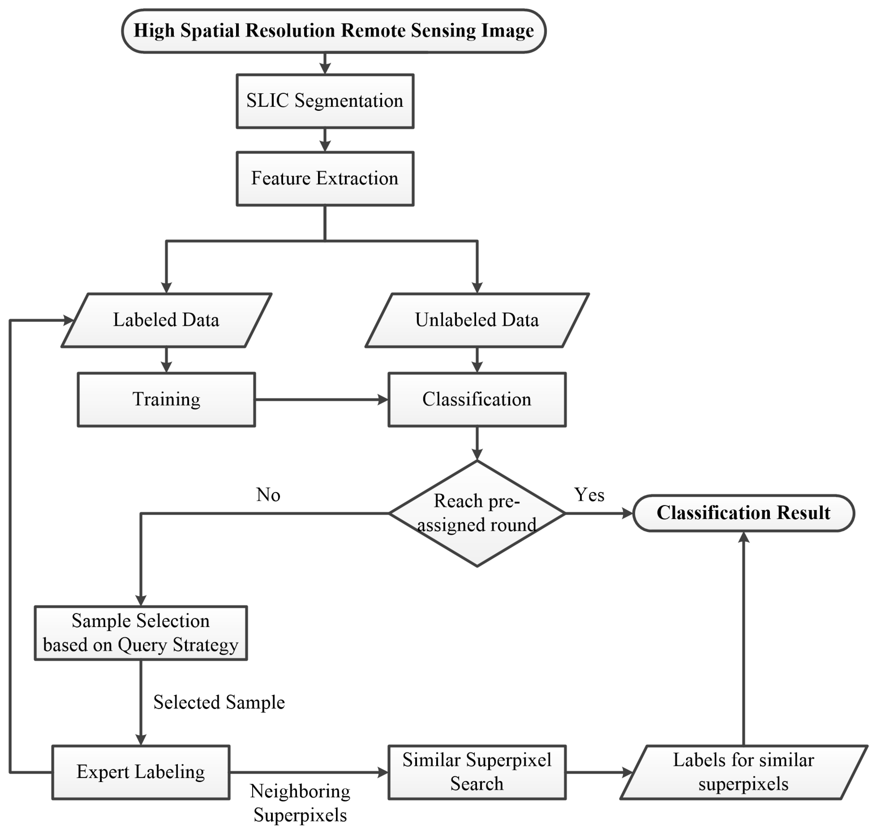
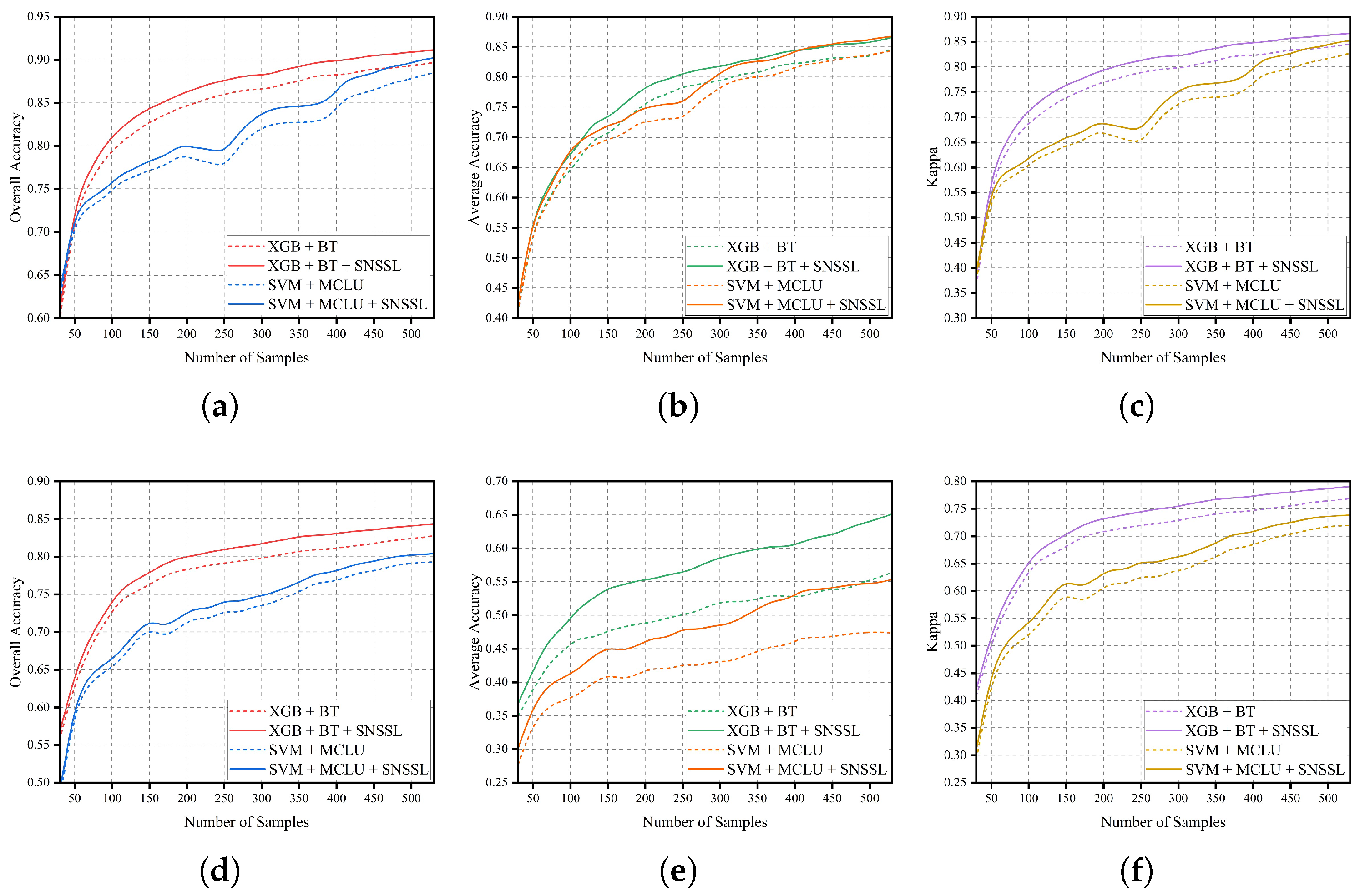
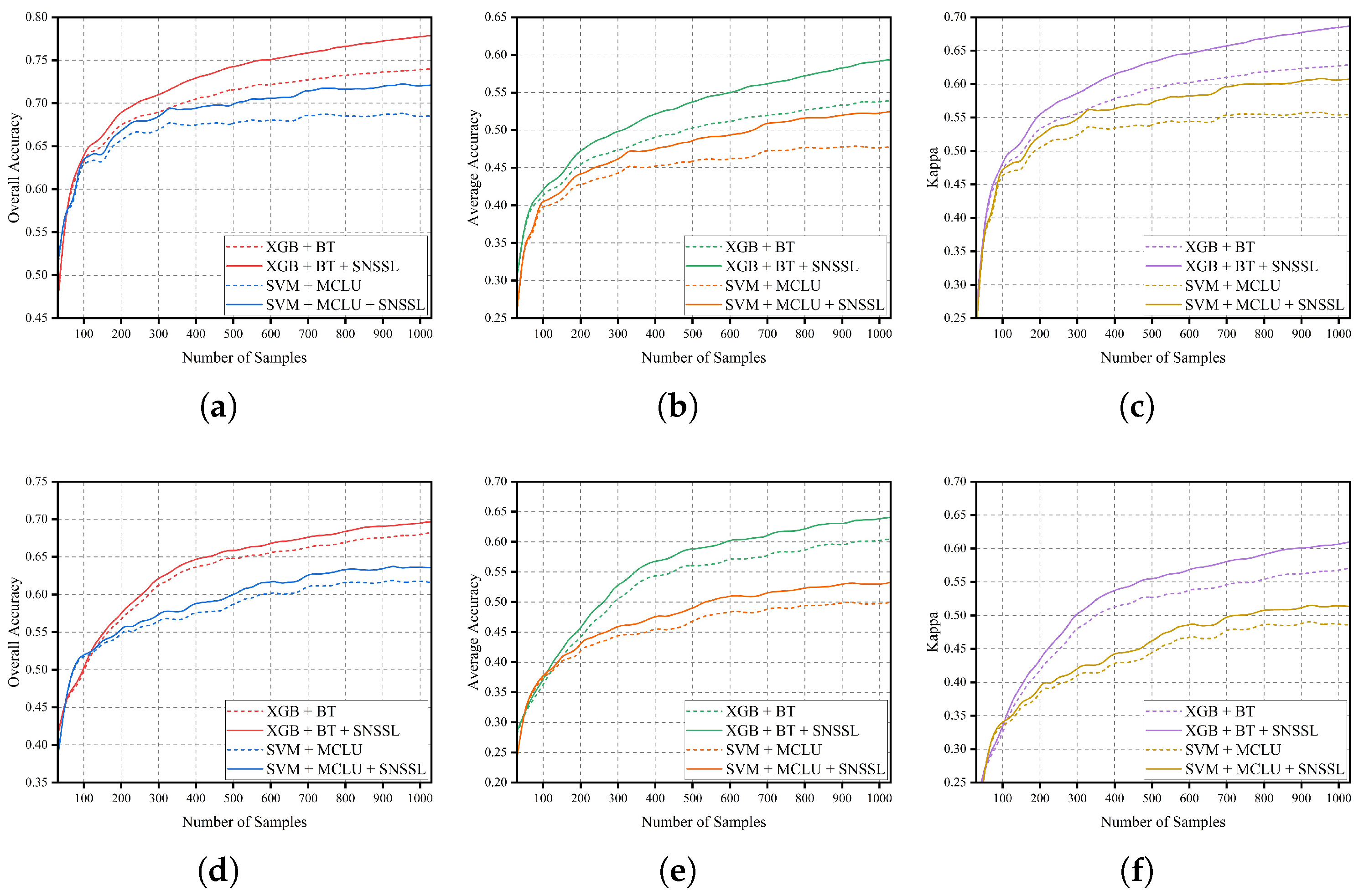
In this paper, we first identify superpixels with certain categories and uncertain superpixels by using supervised learning XGBoost or SVM. Then we use the active learning method to process those uncertain superpixels. We propose the Similar Neighboring Superpixels Search and Labeling (SNSSL) strategy in the AL process to efficiently spread the expert labeling information. The proposed method is innovative in making full use of the expert label information from active learning. The expert labeling information from active learning is only used to enrich the training set for updating the classifier in most papers on active learning. However, in this paper, the expert labeling information from active learning is not only used to enrich the training set but also used to spread the expert label information to similar neighboring superpixels, which is our main contribution. In each round of active query, the most uncertain superpixel (named target superpixel) will be selected for labeling. The neighboring superpixels which are highly similar to the target superpixel will be selected by the search method based on superpixel similarity. Then the label of the target superpixel will be assigned to the selected neighboring superpixels. The main idea behind the method which exploits superpixel-based contextual information is Tobler’s First Law of Geography (near things are more related than distant things) [29]. If two superpixels are spatially close, there is a high probability that the two superpixels belong to the same ground class; therefore, the method propagates the expert label information to spatially adjacent superpixels by computing the similarity between the expert labeled superpixel and its neighbor superpixels. The final classification map is composed of the supervised learning classification map and the active learning with the SNSSL classification map. To demonstrate that the proposed AL method can exploit contextual information and expert labeling information more efficiently, the proposed method is compared with the classifications based on state-of-art AL strategies [4,30] in classification accuracy.
The rest of this article is organized as follows. In Section 2, the details of the proposed method are presented. The experimental results are provided in Section 3, and the discussions are provided in Section 4. In Section 5, the conclusion of our work is presented.

2. Materials and Methods

2.1. Superpixel Based Feature Extraction

As the classification is executed based on superpixels, superpixel segmentation should be conducted first. The Simple Linear Iterative Clustering (SLIC) [31] algorithm is adopted to generate superpixels because of its advantages in simplicity, adherence to boundaries, computational speed, and memory efficiency [32]. After segmentation, features of superpixels will be extracted for classification. In this research, Global Color Histogram (GCH) [33], Local Binary Pattern (LBP) [34], and Gray-level Co-occurrence Matrix (GLCM) [35] are selected to represent the features of superpixels.
GCH is one of the most common and traditional ways to describe the color feature of the image. In this research, the GCH is extracted from the segmented superpixel rather than an image. In a color space with N colors ( C 1 , C 2 , , C N ), the GCH can be represented by a C-dimensional vector ( h 1 , h 2 , , h N ), in which h i represents the percentage occupied by color C i in the superpixel. For a superpixel with the size of M, the h i can be calculated as:
h i = j = 1 M D j M
where D j = 1 if the color of the j-th pixel in the superpixel is as same as the C i , otherwise D j = 0 . The number of colors N used in this research is set as 16 and the color space used to represent color is CIELab color space [36]. That is, each color range in the LAB color space is divided into 16 equal parts, and the percentage of frequencies in each equal part interval is calculated.
Local binary pattern (LBP) has been widely applied to texture classification due to its simplicity, efficiency, and rotation invariant property [34]. Therefore, the LBP histogram is adopted in this paper to represent the first part of the texture feature in the superpixel. Except for LBP, texture features extracted from GLCM [35] are also widely used in classification tasks. The GLCM characterizes the texture of an image by calculating how often pairs of pixels with specific values and in a specified spatial relationship occur in an image. In this research, the GLCM is extracted from superpixels. The features extracted from the GLCM are Homogeneity, Correlation, Contrast, and Angular second moment (ASM). The first two of them are used as texture features of superpixels for classification, and the last three are used as part of the similarity features of superpixels for extending expert labeling information.
As contextual information is important for classification, the features of the neighboring superpixels are also considered. For a target superpixel S t a r g e t having n directly adjacent superpixels, the final feature F F t a r g e t is the integration of its own features F t a r g e t and features of its directly adjacent superpixels ( F 1 , F 2 , , F n ). The F 1 , F 2 , , F n are averaged first, then the averaged features will be concatenated with the F t a r g e t to form the F F t a r g e t . The whole feature extraction process is shown in Figure 1.

2.2. Active Learning Based on Similar Neighboring Superpixel Search and Labeling

2.2.1. Active Learning Query Strategies

The AL query strategy is important for selecting more informative samples from unlabeled data. In this research, Breaking Ties (BT) [30] and MultiClass-Level Uncertain (MCLU) [4] which are commonly used in AL are considered.
BT is usually used when the output of classifiers is class probability. After classification, if there are C classes, a probability vector [ P 1 ( x ) , P 2 ( x ) , , P C ( x ) ] will be generated for each sample. In the probability vector, if the greatest probability is P a ( x ) and the second greatest probability is P b ( x ) , the criterion BT for selecting informative samples is defined as:
B T = P a ( x ) P b ( x )
The most informative sample that should be selected is the sample with the lowest BT.
MCLU is only used for the SVM classifier [37]. During classification, for each sample, the distances to all n hyperplanes [ f 1 ( x ) , f 2 ( x ) , , f n ( x ) ] are calculated. Only the first largest distance value r 1 m a x ( x ) and second largest distance value r 2 m a x ( x ) are considered in the Classification Confidence (CC):
C C = r 1 m a x ( x ) r 2 m a x ( x )
The most informative sample that should be selected is the sample with the lowest CC.

2.2.2. Superpixel Community

In the process of AL, when a target sample is selected for labeling, the similarity between this sample and its neighboring superpixels will be calculated. To spread expert labeling information efficiently, the concept of the superpixel community is used to define the scope of neighboring superpixels. The size of the superpixel community is controlled by the number of layers ( N L a y e r ) of superpixels. The target sample belongs to the 0th layer and its directly adjacent superpixels belong to the 1st layer. For example, superpixel communities with 1, 2, and 3 layers are shown in Figure 2. In Figure 2, the color of the target superpixel is blue and the color of neighboring superpixels is red. Once the superpixel community is confirmed, the similarity search process will only consider superpixels within the superpixel community.

2.2.3. Superpixel Similarity Calculation

To calculate the similarity between superpixels, both the spectral and texture similarity are considered. The spectral similarity is the color difference between CIELAB dominant colors of superpixels. The CIELAB dominant color is the average of all pixels’ CIELAB colors within the superpixel. The normal way to calculate color difference is to calculate the Euclidean distance between different components of the color. However, the calculated distance can’t well match the observation of human eyes. Therefore, the color difference between CIELAB dominant colors is measured by CIEDE2000 Color-Difference Formula [38], which better matches human eyes’ observation. As for texture similarity, three discriminative texture features, Correlation, Angular Second Moment (ASM), and Contrast features extracted from GLCM are used in the calculation. The distances between these three features are calculated using Euclidean distance. Assuming the CIELAB dominant colors distance between two superpixels is D c , correlation distance is C o r r e l a t i o n , ASM distance is A S M , and Contrast distance is C o n t r a s t , the similarity between superpixels ( S i m ) is calculated by:
S i m = D c 2 + C o r r e l a t i o n 2 + A S M 2 + C o n t r a s t 2

2.2.4. Similar Neighboring Superpixels Search and Labeling under Spatial Constraint

If two objects are spatially close, there is a high probability that these two objects belong to the same ground class [29]. Therefore, spatially close superpixels tend to be more similar than spatially far superpixels. To integrate this rule in searching similar superpixels, the graph is introduced. For each superpixel community, a graph is constructed. The center vertex of the graph is the target superpixel S t selected for labeling. There is an edge for any pair of directly adjacent superpixels and the weight of the edge is the calculated similarity. Hence, the similarity between S t and any other superpixel is their shortest weighted distance in the graph. The shortest weighted distance is calculated using Floyd-Warshall algorithm [39]. Once the similarity between S t and all other superpixels in the superpixel community is obtained, a similarity threshold T is used to judge whether the superpixel is similar to S t . If the superpixel is similar to S t , the label of S t will also be assigned to this superpixel. The labels for all searched similar superpixels will be used to generate the final classification result. The whole process of the proposed classification scheme is shown in Figure 3.

3. Data Sets and Experimental Results

3.1. Data Sets

To verify the effectiveness of the proposed method on high spatial resolution remote sensing image classification, two benchmark datasets are selected for experiments. The first dataset is the FloodNet [40], which was collected with a small UAS platform, DJI Mavic Pro quadcopters. All images of the dataset were collected during 30 August–4 September 2017, at Ford Bend County in Texas and other directly impacted areas, after Hurricane Harvey. This dataset contains 2343 RGB images with a spatial resolution of 1.5 cm. As the classification method proposed in this paper focuses on the classification of a single scene, two representative images (FloodNet-6651 and FloodNet-7577) from 2343 images are selected for the experiment. The size of FloodNet-6651 is 4000 × 3000 and the size of FloodNet-7577 is 4592 × 3072 . The original images and ground truth are shown in Figure 4. The numbers of ground-truth pixels for all categories are tabulated in Table 1. Another dataset is the Potsdam dataset [41] which was captured from urban areas. The whole data set contains 38 images with the size of 6000 × 6000 . The spatial resolution is 5 cm. In our experiments, two representative RGB images in the dataset were chosen. The original images (Potsdam-2_10 and Potsdam-3_10) and ground truth are shown in Figure 5. The numbers of ground-truth pixels for all categories are tabulated in Table 2.

3.2. Experimental Results

To validate the performance of the proposed AL model, experiments were conducted on the selected datasets using different AL strategies methods for comparison. In the segmentation process, considering the ground object sizes in the dataset, the superpixel size for images from FloodNet was set as 35 × 35 and the superpixel size for images from Potsdam was set as 20 × 20 . After segmentation, the number of superpixels in FloofNet-6651 and FloodNet-7577 were 9773 and 11,509, and the number of superpixels in Potsdam-2_10 and Potsdam-3_10 were 89,650 and 89,618. A few superpixels called mixed superpixels may contain pixels from different ground classes because SLIC can’t make sure all generated superpixels are pure. For mixed superpixels, the label of the superpixel is determined from the majority voting of the labels of all pixels within the superpixel. The initial number of superpixels in the training set of FloodNet images is 30 and 500 rounds of AL were conducted. The initial number of superpixels in the training set of Potsdam images is 30 and 1000 rounds of AL were conducted. In each round of AL, one superpixel will be selected from unlabeled superpixels and added to the training set. For all images, the initial training samples were randomly selected from all generated superpixels. In the proposed AL model, the layer number of superpixel community N and similarity threshold T are required to be assigned manually. The N and T for the FloodNet dataset were set as 4 and 8 respectively. The N and T for the Potsdam dataset were set as 7 and 12 respectively. As for the classifiers, as both BT and MCLU AL strategies were considered, the XGBoost (XGB) [42] was used for the BT strategy, and SVM was used for the MCLU strategy. For comparison, the classifications with and without the proposed Similar Neighboring Superpixel Search and Labeling (SNSSL) were conducted. Three quantities metrics Overall Accuracy (OA), Average Accuracy (AA), and Kappa coefficient were adopted to evaluate the classification accuracy. To make the results more robust, the reported classification accuracy is averaged with five runs using different sets of randomly selected initial training samples. The details of the classification accuracy of FloodNet images are tabulated in Table 3 and Table 4, and classification maps are shown in Figure 6 and Figure 7. The details of the classification accuracy of Potsdam images are tabulated in Table 5 and Table 6, and classification maps are shown in Figure 8 and Figure 9.
From the accuracy of FloodNet-6651, it can be observed that after adding the proposed SNSSL, the accuracy of all classes increased for both two AL strategies. Specifically, when SNSSL was added in XGB + BT, the accuracy of the Road increased from 82.79% to 85.84%. Moreover, compared with the classification map generated from XGB + BT, the misclassifications of the Road in XGB + BT + SNSSL were obviously reduced. Among all classifications, the XGB + BT + SNSSL achieved the best performance. From the accuracy of FloodNet-7577, after adding SNSSL, the accuracy of almost all classes increased for both AL strategies. Only the accuracy of Tree in XGB + BT decreased slightly after adding SNSSL. For Potsdam-2_10, the accuracy of all classes also increased after using the proposed SNSSL. The accuracy of the car and tree was low because these two classes occupy a low percentage of the whole image. In the AL process, the selection probabilities of these two classes were low. Thus, the classification performance was negatively affected. For Potsdam-3_10, after using the SNSSL, except for clutter/background, the accuracy of XGB + BT for other classes increased.
Overall, it can be concluded that XGB + BT was able to generate better classification than SVM + MCLU. After using SNSSL, the classification performance of almost all classes was improved. Moreover, in terms of quantities metrics (OA, AA, and Kappa coefficient) and visual quality on the classification maps, the method with SNSSL outperformed the method without SNSSL apparently. Therefore, it was proved that the proposed SNSSL is effective to optimize the classification performance.

4. Discussion

4.1. Effect of the Number of Samples on Classification Accuracy

The number of training samples involved in the classification will affect the performance of the classification. In this section, the accuracy of using different numbers of training samples was investigated. Starting from 30 initialized training samples, the classification accuracy was recorded after every 20 rounds of AL. The other settings of the experiments were as same as that used in Section 3.2. The training curves of OA, AA, and Kappa Efficient in FloodNet and Potsdam datasets are shown in Figure 10 and Figure 11, respectively.
It can be observed that the accuracy increased fast at the beginning of AL then the accuracy increase became slower when the number of samples increased. From both Figure 10 and Figure 11, it can be concluded that after using the proposed SNSSL, both the classification accuracy of XGB + BT and SVM + MCLU was improved. In addition, the accuracy of XGB + BT + SNSSL performed best no matter how many training samples were used.

4.2. Effect of the Parameters Setting on Classification Accuracy

In the proposed classification method, both the layer number of Superpixel Community N and the similarity threshold T require to be assigned manually. The layer number of Superpixel Community N will affect the scope of the similar neighboring superpixel search. Moreover, the similarity threshold T will affect the judgment on whether the neighboring superpixel is similar to the target superpixel. Therefore, both the N and T will affect the classification accuracy. In this section, the experiments were conducted using different N and T in the proposed classification method and the classification results were compared. The layer numbers N increased from 1 to 8 with the interval of 1. The similarity threshold T increased from 2 to 16 with an interval of 2. The other settings of the experiments were as same as that used in Section 3.2. In Figure 12 and Figure 13, the classification accuracy of all sets of parameters was displayed in hot maps.
As can be observed in Figure 12, for both methods on FloodNet images, when T increased from 2 to 6, the classification accuracy increased, and when T increased from 10 to 16, the classification accuracy decreased. Therefore, the optimal value of T for FloodNet images was in the range of 6~10. Moreover, when T was in the range of 6~10, the classification accuracy was high if N was higher than 2. Overall, the final optimal parameters for FloodNet images were set as 8 for T and 4 for N. In Figure 13, for both methods on the Potsdam 2_10 image, the classification accuracy increased along with the increase of T. While for both methods on the Potsdam 3_10 image, the classification accuracy increased before T reached 10 and then decreased after T was higher than 12. For both methods on Potsdam 2_10 and Potsdam 3_10 images, when N was higher than 4, the classification accuracy was high. Overall, for both Potsdam 2_10 and Potsdam 3_10 images, the optimal parameters were 12 for T and 7 for N.

5. Conclusions

In this paper, we propose a superpixel-based active learning classification model for high spatial resolution remote sensing imagery. The contextual information between adjacent superpixels is efficiently exploited by the proposed feature extraction process. To make full use of the expert labeling information, the label of the selected sample in AL is not only added to the training set but also assigned to feature similar and spatial close neighboring superpixels. In this way, the expert labeling information will be accurately extended to neighboring superpixels, thus improving the classification accuracy. The experimental results demonstrate that the proposed classification methods outperform the methods using the traditional AL strategies.
Although the superpixel-based classification method can achieve better classification performance than the pixel-based classification method, it still has two shortcomings: (1) there are a few mixed superpixels (under-segmentation) that will result in misclassification, (2) the shape information of superpixels is useless in the classification because most of the superpixels are over-segmented. In the future, we will try to improve the segmentation quality by reducing the under-segmentation in the segmentation result.

Author Contributions

J.T. and H.T. proposed the method and implemented the experiments. J.T. wrote the manuscript. F.T. provided overall guidance of the work and edited the manuscript. Y.Z. and W.C. reviewed and edited the manuscript. All authors have read and agreed to the published version of the manuscript.

Funding

This research was funded by the National Natural Science Foundation of China under grant number 41171339, 61501413 and U1803117.

Data Availability Statement

Publicly available datasets were analyzed in this study. The FloodNet dataset can be found here: [https://drive.google.com/drive/folders/1leN9eWVQcvWDVYwNb2GCo5ML_wBEycWD?usp=sharing]. The Potsdam dataset can be found here: [https://www.isprs.org/education/benchmarks/UrbanSemLab/default.aspx].

Conflicts of Interest

The authors declare no conflict of interest.

References

  1. Settles, B. Active Learning Literature Survey; Computer Sciences Technical Report 1648; University of Wisconsin–Madison: Madison, WI, USA, 2009. [Google Scholar]
  2. Aggarwal, C.C.; Kong, X.; Gu, Q.; Han, J.; Philip, S.Y. Active learning: A survey. In Data Classification; Chapman and Hall/CRC: Boca Raton, FL, USA, 2014; pp. 599–634. [Google Scholar]
  3. Kumar, P.; Gupta, A. Active learning query strategies for classification, regression, and clustering: A survey. J. Comput. Sci. Technol. 2020, 35, 913–945. [Google Scholar] [CrossRef]
  4. Demir, B.; Persello, C.; Bruzzone, L. Batch-mode active-learning methods for the interactive classification of remote sensing images. IEEE Trans. Geosci. Remote Sens. 2010, 49, 1014–1031. [Google Scholar] [CrossRef] [Green Version]
  5. Xu, J.; Hang, R.; Liu, Q. Patch-based active learning (PTAL) for spectral-spatial classification on hyperspectral data. Int. J. Remote Sens. 2014, 35, 1846–1875. [Google Scholar] [CrossRef]
  6. Wang, Z.; Du, B.; Zhang, L.; Zhang, L.; Jia, X. A novel semisupervised active-learning algorithm for hyperspectral image classification. IEEE Trans. Geosci. Remote Sens. 2017, 55, 3071–3083. [Google Scholar] [CrossRef]
  7. Hay, G.J.; Castilla, G. Geographic Object-Based Image Analysis (GEOBIA): A new name for a new discipline. In Object-Based Image Analysis; Springer: Berlin/Heidelberg, Germany, 2008; pp. 75–89. [Google Scholar]
  8. Cheng, J.; Bo, Y.; Zhu, Y.; Ji, X. A novel method for assessing the segmentation quality of high-spatial resolution remote-sensing images. Int. J. Remote Sens. 2014, 35, 3816–3839. [Google Scholar] [CrossRef]
  9. Hossain, M.D.; Chen, D. Segmentation for Object-Based Image Analysis (OBIA): A review of algorithms and challenges from remote sensing perspective. ISPRS J. Photogramm. Remote Sens. 2019, 150, 115–134. [Google Scholar] [CrossRef]
  10. Myint, S.W.; Gober, P.; Brazel, A.; Grossman-Clarke, S.; Weng, Q. Per-pixel vs. object-based classification of urban land cover extraction using high spatial resolution imagery. Remote Sens. Environ. 2011, 115, 1145–1161. [Google Scholar] [CrossRef]
  11. Fu, Z.; Sun, Y.; Fan, L.; Han, Y. Multiscale and multifeature segmentation of high-spatial resolution remote sensing images using superpixels with mutual optimal strategy. Remote Sens. 2018, 10, 1289. [Google Scholar] [CrossRef] [Green Version]
  12. Sun, H.; Ren, J.; Zhao, H.; Yan, Y.; Zabalza, J.; Marshall, S. Superpixel based feature specific sparse representation for spectral-spatial classification of hyperspectral images. Remote Sens. 2019, 11, 536. [Google Scholar] [CrossRef] [Green Version]
  13. Huang, W.; Huang, Y.; Wang, H.; Liu, Y.; Shim, H.J. Local binary patterns and superpixel-based multiple kernels for hyperspectral image classification. IEEE J. Sel. Top. Appl. Earth Obs. Remote Sens. 2020, 13, 4550–4563. [Google Scholar] [CrossRef]
  14. Chen, Y.; Ming, D.; Lv, X. Superpixel based land cover classification of VHR satellite image combining multi-scale CNN and scale parameter estimation. Earth Sci. Inform. 2019, 12, 341–363. [Google Scholar] [CrossRef]
  15. Zhang, S.; Li, C.; Qiu, S.; Gao, C.; Zhang, F.; Du, Z.; Liu, R. EMMCNN: An ETPS-based multi-scale and multi-feature method using CNN for high spatial resolution image land-cover classification. Remote Sens. 2019, 12, 66. [Google Scholar] [CrossRef] [Green Version]
  16. Xie, F.; Gao, Q.; Jin, C.; Zhao, F. Hyperspectral image classification based on superpixel pooling convolutional neural network with transfer learning. Remote Sens. 2021, 13, 930. [Google Scholar] [CrossRef]
  17. Li, Z.; Li, E.; Samat, A.; Xu, T.; Liu, W.; Zhu, Y. An Object-Oriented CNN Model Based on Improved Superpixel Segmentation for High-Resolution Remote Sensing Image Classification. IEEE J. Sel. Top. Appl. Earth Obs. Remote Sens. 2022, 15, 4782–4796. [Google Scholar] [CrossRef]
  18. Li, L.; Han, L.; Miao, Q.; Zhang, Y.; Jing, Y. Superpixel-Based Long-Range Dependent Network for High-Resolution Remote-Sensing Image Classification. Land 2022, 11, 2028. [Google Scholar] [CrossRef]
  19. Diao, Q.; Dai, Y.; Zhang, C.; Wu, Y.; Feng, X.; Pan, F. Superpixel-based attention graph neural network for semantic segmentation in aerial images. Remote Sens. 2022, 14, 305. [Google Scholar] [CrossRef]
  20. Dong, Y.; Liu, Q.; Du, B.; Zhang, L. Weighted feature fusion of convolutional neural network and graph attention network for hyperspectral image classification. IEEE Trans. Image Process. 2022, 31, 1559–1572. [Google Scholar] [CrossRef] [PubMed]
  21. Zhu, W.; Zhao, C.; Feng, S.; Qin, B. Multiscale short and long range graph convolutional network for hyperspectral image classification. IEEE Trans. Geosci. Remote Sens. 2022, 60, 1–15. [Google Scholar] [CrossRef]
  22. Guo, J.; Zhou, X.; Li, J.; Plaza, A.; Prasad, S. Superpixel-based active learning and online feature importance learning for hyperspectral image analysis. IEEE J. Sel. Top. Appl. Earth Obs. Remote Sens. 2016, 10, 347–359. [Google Scholar] [CrossRef]
  23. Liu, W.; Yang, J.; Li, P.; Han, Y.; Zhao, J.; Shi, H. A novel object-based supervised classification method with active learning and random forest for PolSAR imagery. Remote Sens. 2018, 10, 1092. [Google Scholar] [CrossRef] [Green Version]
  24. Breiman, L. Random forests. Mach. Learn. 2001, 45, 5–32. [Google Scholar] [CrossRef] [Green Version]
  25. Ma, L.; Fu, T.; Li, M. Active learning for object-based image classification using predefined training objects. Int. J. Remote Sens. 2018, 39, 2746–2765. [Google Scholar] [CrossRef]
  26. Su, T.; Zhang, S.; Liu, T. Multi-spectral image classification based on an object-based active learning approach. Remote Sens. 2020, 12, 504. [Google Scholar] [CrossRef] [Green Version]
  27. Csillik, O. Fast segmentation and classification of very high resolution remote sensing data using SLIC superpixels. Remote Sens. 2017, 9, 243. [Google Scholar] [CrossRef] [Green Version]
  28. Tong, H.; Tong, F.; Zhou, W.; Zhang, Y. Purifying SLIC superpixels to optimize superpixel-based classification of high spatial resolution remote sensing image. Remote Sens. 2019, 11, 2627. [Google Scholar] [CrossRef] [Green Version]
  29. Tobler, W.R. A computer movie simulating urban growth in the Detroit region. Econ. Geogr. 1970, 46, 234–240. [Google Scholar] [CrossRef]
  30. Luo, T.; Kramer, K.; Goldgof, D.B.; Hall, L.O.; Samson, S.; Remsen, A.; Hopkins, T.; Cohn, D. Active learning to recognize multiple types of plankton. J. Mach. Learn. Res. 2005, 6, 589–613. [Google Scholar]
  31. Achanta, R.; Shaji, A.; Smith, K.; Lucchi, A.; Fua, P.; Süsstrunk, S. SLIC superpixels compared to state-of-the-art superpixel methods. IEEE Trans. Pattern Anal. Mach. Intell. 2012, 34, 2274–2282. [Google Scholar] [CrossRef] [Green Version]
  32. Stutz, D.; Hermans, A.; Leibe, B. Superpixels: An evaluation of the state-of-the-art. Comput. Vis. Image Underst. 2018, 166, 1–27. [Google Scholar] [CrossRef] [Green Version]
  33. Yue, J.; Li, Z.; Liu, L.; Fu, Z. Content-based image retrieval using color and texture fused features. Math. Comput. Model. 2011, 54, 1121–1127. [Google Scholar] [CrossRef]
  34. Wang, Y.; Zhao, Y.; Chen, Y. Texture classification using rotation invariant models on integrated local binary pattern and Zernike moments. EURASIP J. Adv. Signal Process. 2014, 2014, 182. [Google Scholar] [CrossRef] [Green Version]
  35. Haralick, R.M.; Shanmugam, K.; Dinstein, I.H. Textural features for image classification. IEEE Trans. Syst. Man Cybern. 1973, SMC-3, 610–621. [Google Scholar] [CrossRef] [Green Version]
  36. Connolly, C.; Fleiss, T. A study of efficiency and accuracy in the transformation from RGB to CIELAB color space. IEEE Trans. Image Process. 1997, 6, 1046–1048. [Google Scholar] [CrossRef] [PubMed]
  37. Tuia, D.; Pacifici, F.; Kanevski, M.; Emery, W.J. Classification of very high spatial resolution imagery using mathematical morphology and support vector machines. IEEE Trans. Geosci. Remote Sens. 2009, 47, 3866–3879. [Google Scholar] [CrossRef]
  38. Luo, M.R.; Cui, G.; Rigg, B. The development of the CIE 2000 colour-difference formula: CIEDE2000. Color Res. Appl. 2001, 26, 340–350. [Google Scholar] [CrossRef]
  39. Floyd, R.W. Algorithm 97: Shortest path. Commun. ACM 1962, 5, 345. [Google Scholar] [CrossRef]
  40. Rahnemoonfar, M.; Chowdhury, T.; Sarkar, A.; Varshney, D.; Yari, M.; Murphy, R.R. Floodnet: A high resolution aerial imagery dataset for post flood scene understanding. IEEE Access 2021, 9, 89644–89654. [Google Scholar] [CrossRef]
  41. Rottensteiner, F.; Sohn, G.; Jung, J.; Gerke, M.; Baillard, C.; Benitez, S.; Breitkopf, U. The ISPRS benchmark on urban object classification and 3D building reconstruction. ISPRS Ann. Photogramm. Remote Sens. Spat. Inf. Sci. 2012, I-3, 293–298. [Google Scholar] [CrossRef] [Green Version]
  42. Chen, T.; Guestrin, C. XGBoost: A Scalable Tree Boosting System. In Proceedings of the 22nd ACM SIGKDD International Conference on Knowledge Discovery and Data Mining, KDD’16, San Francisco, CA, USA, 13–17 August 2016; ACM: New York, NY, USA, 2016; pp. 785–794. [Google Scholar] [CrossRef] [Green Version]
Figure 1. Superpixel-based feature extraction process.
Remotesensing 15 00715 g001
Figure 2. Superpixel community examples.
Remotesensing 15 00715 g002
Figure 3. Flowchart of the proposed classification scheme.
Remotesensing 15 00715 g003
Figure 4. Images from FloodNet: (a) 6651 RGB; (b) 6651 ground truth; (c) 7577 RGB; (d) 7577 ground truth.
Remotesensing 15 00715 g004
Figure 5. Images from Potsdam: (a) 2_10 RGB; (b) 2_10 ground truth; (c) 3_10 RGB; (d) 3_10 ground truth.
Remotesensing 15 00715 g005aRemotesensing 15 00715 g005b
Figure 6. Classification maps generated from FloodNet-6651: (a) ground truth; (b) XGB + BT; (c) XGB + BT + SNSSL; (d) class label; (e) SVM + MCLU; (f) SVM + MCLU + SNSSL.
Remotesensing 15 00715 g006aRemotesensing 15 00715 g006b
Figure 7. Classification maps generated from FloodNet-7577: (a) ground truth; (b) XGB + BT; (c) XGB + BT + SNSSL; (d) class label; (e) SVM + MCLU; (f) SVM + MCLU + SNSSL.
Remotesensing 15 00715 g007
Figure 8. Classification maps generated from Potsdam-2_10: (a) ground truth; (b) XGB + BT; (c) XGB + BT + SNSSL; (d) class label; (e) SVM + MCLU; (f) SVM + MCLU + SNSSL.
Remotesensing 15 00715 g008
Figure 9. Classification maps generated from Potsdam-3_10: (a) ground truth; (b) XGB + BT; (c) XGB + BT + SNSSL; (d) class label; (e) SVM + MCLU; (f) SVM + MCLU + SNSSL.
Remotesensing 15 00715 g009aRemotesensing 15 00715 g009b
Figure 10. Training curves of FloodNet images: (a) OA of 6651; (b) AA of 6651; (c) Kappa of 6651; (d) OA of 7577; (e) AA of 7577; (f) Kappa of 7577.
Remotesensing 15 00715 g010
Figure 11. Training curves of Potsdam images: (a) OA of 2_10; (b) AA of 2_10; (c) Kappa of 2_10; (d) OA of 3_10; (e) AA of 3_10; (f) Kappa of 3_10.
Remotesensing 15 00715 g011
Figure 12. OA of the FloodNet images using different sets of parameters: (a) SVM + MCLU + SNSSL on 6651; (b) XGB + BT + SNSSL on 6651; (c) SVM + MCLU + SNSSL on 7577; (d) XGB + BT + SNSSL on 7577.
Remotesensing 15 00715 g012
Figure 13. OA of the Potsdam images using different sets of parameters: (a) SVM + MCLU + SNSSL on 2_10; (b) XGB + BT + SNSSL on 2_10; (c) SVM + MCLU + SNSSL on 3_10; (d) XGB + BT + SNSSL on 3_10.
Remotesensing 15 00715 g013
Table 1. Numbers of ground-truth pixels for all categories in two selected images from FloodNet.
FloodNet-6651FloodNet-7577
Pixel NumberPercentagePixel NumberPercentage
Building1,731,04414.4%2,668,24518.9%
Road-flooded--3,077,13121.8%
Road1,201,78510.0%203,7651.4%
Tree3,048,55525.4%3,421,01624.3%
Vehicle156,4701.3%80,0090.6%
Grass5,862,14648.9%4,606,92732.7%
Pool--49,5310.4%
Table 2. Numbers of ground-truth pixels for all categories in two selected images from Potsdam.
Potsdam-2_10Potsdam-3_10
Pixel NumberPercentagePixel NumberPercentage
Impervious surfaces4,944,59913.7%8,338,19823.2%
Building5,447,00715.1%5,128,14914.2%
Low vegetation15,182,06142.2%11,428,32631.7%
Tree2,679,3887.4%8,780,24524.4%
Car313,1480.9%434,6151.2%
Clutter/background7,433,79720.6%1,890,4675.3%
Table 3. Classification accuracy (averaged on 5 runs) of the FloodNet-6651.
ClassXGB + BTXGB + BT + SNSSLSVM + MCLUSVM + MCLU + SNSSL
Building90.3891.4587.0388.95
Road82.7985.8481.0683.33
Tree88.5490.3787.7090.36
Vehicle69.5772.3174.8678.71
Grass92.0793.0591.2992.23
OA (%)89.7191.1588.5390.22
AA (%)84.6786.6084.3986.72
Kappa × 10084.5486.7082.7785.28
Table 4. Classification accuracy (averaged on 5 runs) of the FloodNet-7577.
ClassXGB + BTXGB + BT + SNSSLSVM + MCLUSVM + MCLU + SNSSL
Building90.8292.4891.8092.08
Road-flooded82.8084.1877.9580.19
Road11.5833.1006.51
Tree85.9485.9376.6277.31
Vehicle19.7825.835.1424.27
Grass80.6382.2680.2081.35
Pool23.4052.20025.86
OA (%)82.7484.3779.4980.55
AA (%)56.4265.1447.3955.37
Kappa × 10076.8879.0872.3573.85
Table 5. Classification accuracy (averaged on 5 runs) of the Potsdam-2_10.
ClassXGB + BTXGB + BT + SNSSLSVM + MCLUSVM + MCLU + SNSSL
Impervious surfaces63.8070.9566.7476.24
Building73.3780.2877.3378.96
Low vegetation90.6291.1386.7388.11
Tree5.5415.2804.56
Car15.6819.782.108.18
Clutter/background74.5278.7453.5258.74
OA (%)74.0277.8968.5172.11
AA (%)53.9259.3647.7452.46
Kappa × 10062.9268.7055.4760.77
Table 6. Classification accuracy (averaged on 5 runs) of the Potsdam-3_10.
ClassXGB + BTXGB + BT + SNSSLSVM + MCLUSVM + MCLU + SNSSL
Impervious surfaces56.7267.5245.1766.57
Building75.6979.1058.9961.43
Low vegetation69.8371.4474.7077.74
Tree53.7259.7535.5539.19
Car28.6628.981.995.47
Clutter/background78.3377.5676.2376.76
OA (%)68.2069.7061.6063.57
AA (%)60.4964.0650.0153.29
Kappa × 10057.0660.9748.6251.34
Disclaimer/Publisher’s Note: The statements, opinions and data contained in all publications are solely those of the individual author(s) and contributor(s) and not of MDPI and/or the editor(s). MDPI and/or the editor(s) disclaim responsibility for any injury to people or property resulting from any ideas, methods, instructions or products referred to in the content.

