
Simulated Trends in Land Surface Sensible Heat Flux on the Tibetan Plateau in Recent Decades

1
Collaborative Innovation Center on Forecast and Evaluation of Meteorological Disasters/Nanjing University of Information Science and Technology, Nanjing 210044, China
2
School of Atmospheric Sciences, Nanjing University of Information Science and Technology, Nanjing 210044, China
3
Land-Atmosphere Interaction and Its Climatic Effects Group, State Key Laboratory of Tibetan Plateau Earth System, Resources and Environment (TPESRE), Institute of Tibetan Plateau Research, Chinese Academy of Sciences, Beijing 100101, China
4
College of Earth and Planetary Sciences, University of Chinese Academy of Sciences, Beijing 100049, China
5
College of Atmospheric Sciences, Lanzhou University, Lanzhou 730000, China
6
National Observation and Research Station for Qomolangma Special Atmospheric Processes and Environmental Changes, Dingri 858200, China
7
Kathmandu Center of Research and Education, Chinese Academy of Sciences, Beijing 100101, China
8
China-Pakistan Joint Research Center on Earth Sciences, Chinese Academy of Sciences, Islamabad 45320, Pakistan
*
Author to whom correspondence should be addressed.
Remote Sens. 2023, 15(3), 714; https://doi.org/10.3390/rs15030714
Submission received: 15 December 2022
/
Revised: 13 January 2023
/
Accepted: 18 January 2023
/
Published: 25 January 2023
(This article belongs to the Special Issue Land-Atmosphere Interactions and Effects on the Climate of the Tibetan Plateau and Surrounding Regions II)
Abstract
:The spatial distribution and temporal variation of land surface sensible heat (SH) flux on the Tibetan Plateau (TP) for the period of 1981–2018 were studied using the simulation results from the Noah-MP land surface model. The simulated SH fluxes were also compared with the simulation results from the SEBS model and the results derived from 80 meteorological stations. It is found that, much larger annual mean SH fluxes occurred on the western and central TP compared with the eastern TP. Meanwhile, the inter-annual variations of SH fluxes on the central and western TP were larger than that on the eastern TP. The SEBS simulation showed much larger inter-annual variations than did the Noah-MP simulation across most of the TP. There was a trend of decrease in SH flux from the mid-1980s to the beginning of the 21st century in the Noah-MP simulations. Both Noah-MP and SEBS showed an increasing SH flux trend after this period of decrease. The increasing trend appeared on the eastern TP later than on the western and central TP. In the Noah-MP simulation, the western and central TP showed larger values of temperature difference between the ground surface and air (Ts–Ta) than did the eastern TP. Both mean Ts–Ta and wind speed decreased from the mid-1980s to approximately 2000, and then increased slightly. However, the Ts–Ta transition occurred later than that of wind speed. Changes in mean ground surface temperature (Ts) were the main cause of the decreasing and increasing trends in SH flux on the TP. Meanwhile, changes in wind speed contributed substantially to the decreasing trend in SH flux before 1998.
1. Introduction
As the Earth’s third pole, the Tibetan Plateau (TP) plays a critical role in influencing regional and global climate. Over the past few decades, the TP has experienced evident climate change, which has contributed to amplifying environmental changes on the global scale. The large heat source in the mid-troposphere provided by the TP is perceived as an important factor contributing to the formation and variation of the Asian summer monsoon [1,2,3]. Land surface sensible heat (SH) flux is a major component of this heat source, and plays a considerable role in modulating large scale atmospheric circulation and the summer monsoon precipitation patterns [4,5,6,7,8,9]. Hence, many studies have attempted to estimate the spatiotemporal changes in SH flux over the TP using meteorological data [10,11,12,13], reanalysis data [14,15,16], remote sensing products [17,18,19] or model simulations [20,21].
Duan and Wu [10] calculated the SH flux on the TP for the period 1980–2003 using data from meteorological stations and satellites. They found that the SH flux on the TP exhibited a large diurnal range, but much smaller annual range. The SH flux also showed a significant decreasing trend from the mid-1980s to the beginning of the 21st century, with a subdued surface wind speed contributing highly to the decreasing trend. Further, Duan et al. [11] reexamined the SH flux trend during 1980–2008, and confirmed the weakening trend. They found that the trend was induced mainly by a reduction in surface wind speed, despite a sharp increase in the ground-air temperature difference in 2004–2008. They also considered the trend to be a primary response to the spatial nonuniformity of large scale warming over the East Asian continent. Yang et al. [13] investigated the differences between different methods in estimating SH flux trends on the TP using meteorological station data for the period 1984–2006. Their results showed that different schemes produced different trends, and they claimed that the SH flux on the TP weakened by 2% per decade using their own newly developed method. They suggested that a decrease in wind speed and increase in ground–air temperature difference may moderate the trend of the heat transfer coefficient, which in turn may influence the SH flux trend. Wang and Ma [21] performed several simulation experiments on the TP using the Noah-MP land surface model. Their results showed that the SH flux is very sensitive to the thermal roughness length parameterization scheme, and also supported the SH flux weakening trend from the mid-1980s onwards.
However, the SH flux weakening trend did not continue during the last decade [22,23,24,25]. Zhang et al. [23] calculated the SH flux over the TP from 1970 to 2015 using meteorological station data, and analyzed the temporal characteristics of SH flux. They pointed out that there was an increasing trend in SH flux during the period 2001–2015. Chen et al. [25] investigated the spatiotemporal variability in SH over the TP from 1980 to 2015 using data from meteorological station and reanalysis products. They also confirmed that an increasing trend followed the earlier decreasing trend, and stated that the declines in SH prior to 2000 resulted from changes in wind speed, while the subsequent recovery can be attributed to increases in both wind speed and air–surface temperature gradient.
Most previous studies estimated the SH flux on the TP using reanalysis datasets or meteorological station data from the China Meteorological Administration (CMA), and bulk transfer algorithms. There are many uncertainties in estimating the SH flux on the TP using data from unevenly distributed meteorological stations and/or diverse reanalysis datasets. Hence, the decadal SH flux trends, especially when and how the trends changed, remain controversial. This study presents high resolution simulations of SH flux using the Noah-MP land surface model and SEBS (surface energy balance system) model, and compares these with the results from CMA meteorological stations. The climatic features of SH flux on the TP and possible causes of the annual variation trends are then analyzed. In the next section, observations and the experimental design will be described.
2. Materials and Methods
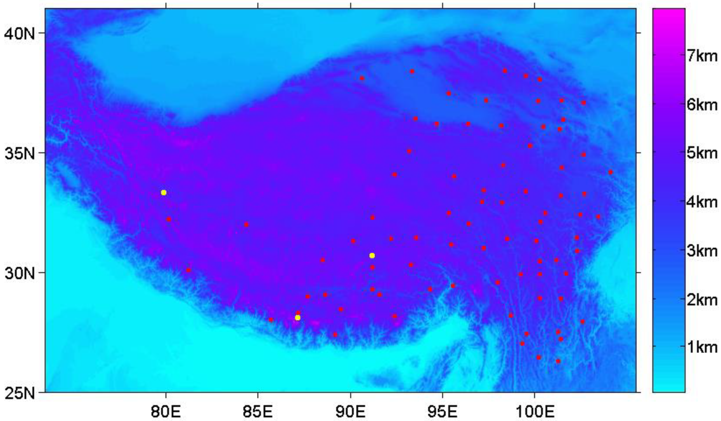
To evaluate the simulation results from the Noah-MP model, SH flux datasets collected from the eddy covariance (EC) systems at three observation stations were used. The QOMS station is situated at the bottom of the lower Rongbuk Valley, to the north of Mt. Everest; here, the EC system was installed at a height of 3.25 m above ground level. The Nam Co station is located on the southeast shore of the Nam Co Lake on the central TP; here, the EC system was installed at a height of 3.06 m above ground level. The Ali station is located within a flat and open mountain valley on the northwestern TP, where the Indian monsoon and westerly wind interact intensively; here, the EC system was installed at a height of 2.75 m above ground level. Figure 1 shows the locations of the stations (yellow dots), and Table 1 gives the observation periods and EC system information. The details of the stations and data have been introduced in previous studies [26,27]. All the datasets were quality-controlled using the TK3 software [28].
The Noah-MP land surface model was developed from the Noah land surface model (version 3.0) with multiple parameterization options [29,30]. This model is suitable for land surface process simulation over the TP according to previous studies [31,32]. In our simulation, the SIMGM runoff scheme, Noah β-factor scheme, and BATS snow surface albedo scheme were selected. Table 2 gives the schemes for the key processes.
The thermal roughness length scheme proposed by Zeng and Dickinson [33] was selected for our simulation experiment, because this scheme provided the best estimation of monthly mean SH flux in terms of squared correlation coefficients [21]. The simulation experiment was conducted at a spatial resolution of 0.1° and temporal resolution of 3 h using the CMFD (China meteorological forcing dataset) data [34] as the atmospheric forcing dataset for the TP area. The Noah-MP model was run continuously for the period from 1 January 1981 to 31 December 2018. The 38-yr simulation results were calculated and analyzed in this study.
We also used the 18-yr dataset produced by the SEBS model, which was developed by Su [35] and updated by Chen et al. [36] and Han et al. [37,38]. In the process of calculating the turbulent flux, the sub-grid scale topography drag parameterization scheme was introduced to improve the simulation of SH flux [39]. The simulation was conducted for the period 2001–2018 based on satellite remote sensing data (MODIS) and meteorological data (CMFD). The MODIS monthly land surface products, including land surface temperature and emissivity, land surface albedo, and vegetation index, provides the land surface conditions for the SEBS model. The SH flux was computed using the Monin-Obukhov similarity theory. The values of land surface variables in the MODIS monthly products were derived by compositing and averaging the values from the corresponding month of MODIS daily files. Detailed information on the MODIS land surface variables is listed in Table 3.
The simulated SH fluxes from the two models were also compared with the SH flux dataset estimated using routine meteorological data from CMA stations. This CMA station-based dataset was provided by Duan et al. [40], and was derived from 80 CMA stations (Figure 1) using a physical method developed by Yang et al. [41]. The daily mean heat flux is calculated by
where ρ is air density, cp is the specific heat at a constant pressure, u is the wind speed at a reference level, Ts is the ground surface temperature, Ta is the air temperature at a reference level, and CH is the heat transfer coefficient. CH is not a given constant value, and its value can be obtained by different parameterization schemes [42].
In this method, CH is determined from micro-meteorological theory and experimental analysis. It exhibits clear diurnal variations, which significantly affect the estimation of SH flux [41]. This method (hereafter, the Yang method) produces higher SH fluxes than conventional empirical methods that are widely used in climatological studies [25,43,44].
To assess the simulations, we used statistical methods including the correlation coefficient, squared correlation coefficient (R2), linear least-squares regression, and Mann–Kendall trend test.
3. Results
3.1. Assessment of the Simulation
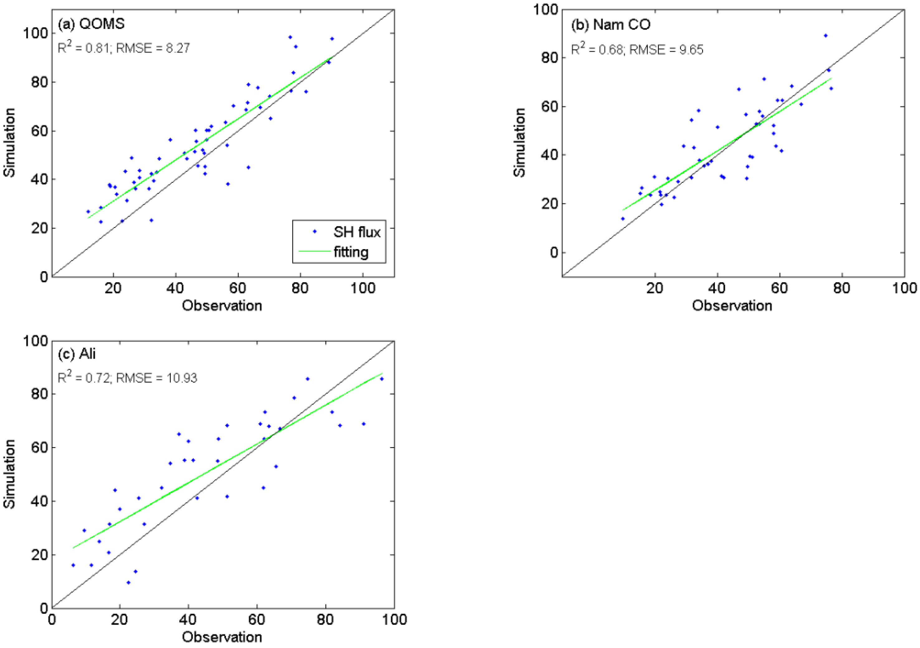
Before analyzing the trends in simulated SH flux, a validation was performed using the in-situ observation data at the 3 stations. The linear regression method was applied here. Figure 2a shows the comparison between simulated and observed monthly mean SH fluxes at the QOMS station for 5 yrs (2011–2015). The blue dots represent the monthly mean values, and the blue line is the best-fit line. The squared correlation coefficient (R2) was 0.81, with a root-mean-square error (RMSE) of 8.27 Wm−2. Overall, the simulated SH fluxes were higher than the corresponding observations. At the Nam Co station, there were many missing observations in the dataset during the observation period (2011–2015). Hence, the mean values of SH flux in 5 months were not obtained. The R2 was 0.68, with a RMSE of 9.65 Wm−2. The simulated mean SH fluxes fit well with observations during the equivalent period (Figure 2b). Figure 2c show the comparison between simulated and observed monthly mean SH fluxes at the Ali station for 5 yrs (2011–2015). As there were many missing values in the dataset, only 36 monthly mean values were obtained here. The R2 was 0.72, and the RMSE was larger those at the other two stations.
Han et al. [38,39] previously evaluated the dataset produced by SEBS during the period 2007–2012. The SH flux was underestimated, with a mean bias of 4.7 Wm−2 at the QOMS station, and 7.8 Wm−2 at the Nam Co station. The correlation coefficients between the SEBS simulation and EC observations were 0.41 at the QOMS station, and 0.63 at the Nam Co station, respectively.
3.2. Simulated SH Flux and Its Trends
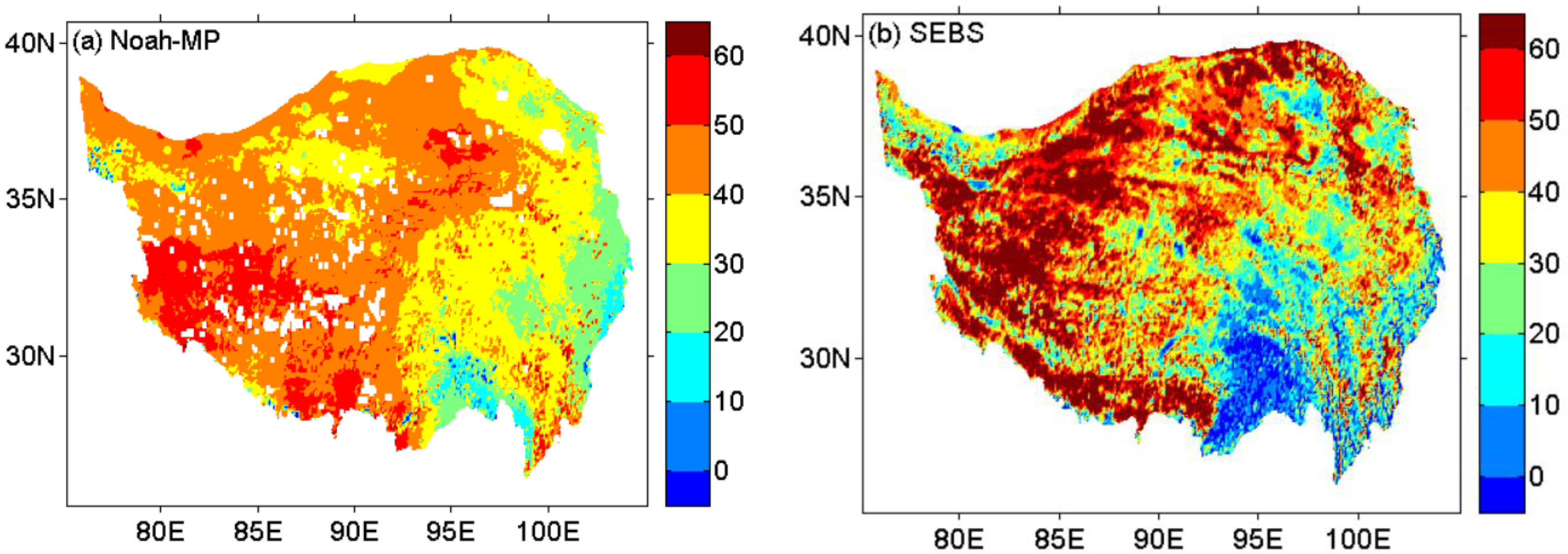
From the analysis performed in the section above, the simulations of SH flux were deemed to be suitable overall. The spatial distribution of annual mean SH flux (2001–2018) based on Noah-MP is shown in Figure 3a, and the corresponding SEBS-based annual mean SH flux is shown in Figure 3b. In Figure 3a, it can be seen that the eastern TP received much weaker mean SH fluxes than the central and western TP during the period 2001–2018. The areas with mean SH fluxes greater than 50 Wm−2 were mainly in the southwestern TP region. In the SEBS simulation (Figure 3b), most areas of the western TP received more than 60 Wm−2 SH fluxes. Overall, SEBS gave larger SH flux values in the northwestern TP region, but smaller SH flux values in the southeastern TP region than did Noah-MP.
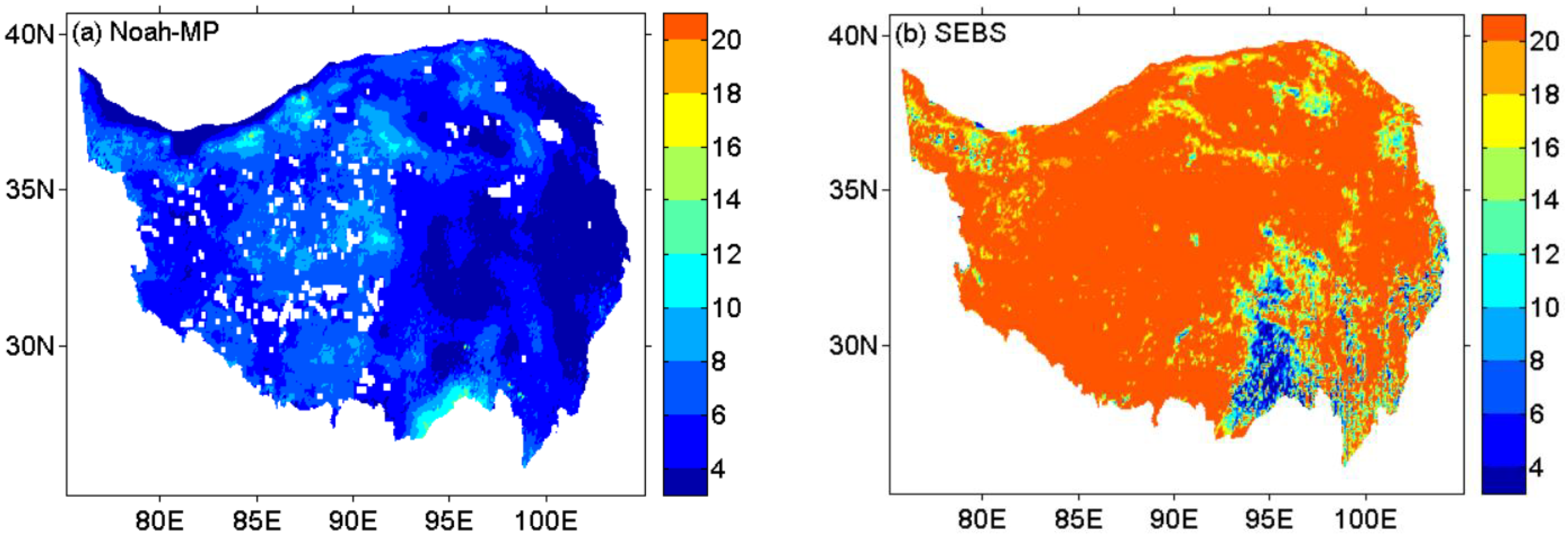
Figure 4 shows the variations in the annual mean SH flux during the period 2001–2018. A large standard deviation (STD) value indicates large inter-annual variation in the SH flux, and vice versa. In the Noah-MP simulation (Figure 4a), large STD values were mainly observed over the central and western TP, while small STD values were mainly observed over areas to the east of 92°E. This means that the central and western TP recorded larger inter-annual variations in SH flux than did the eastern TP. The SEBS simulation (Figure 4b) showed much larger inter-annual variation in SH flux than did the Noah-MP simulation (Figure 4a) in most areas of the TP.
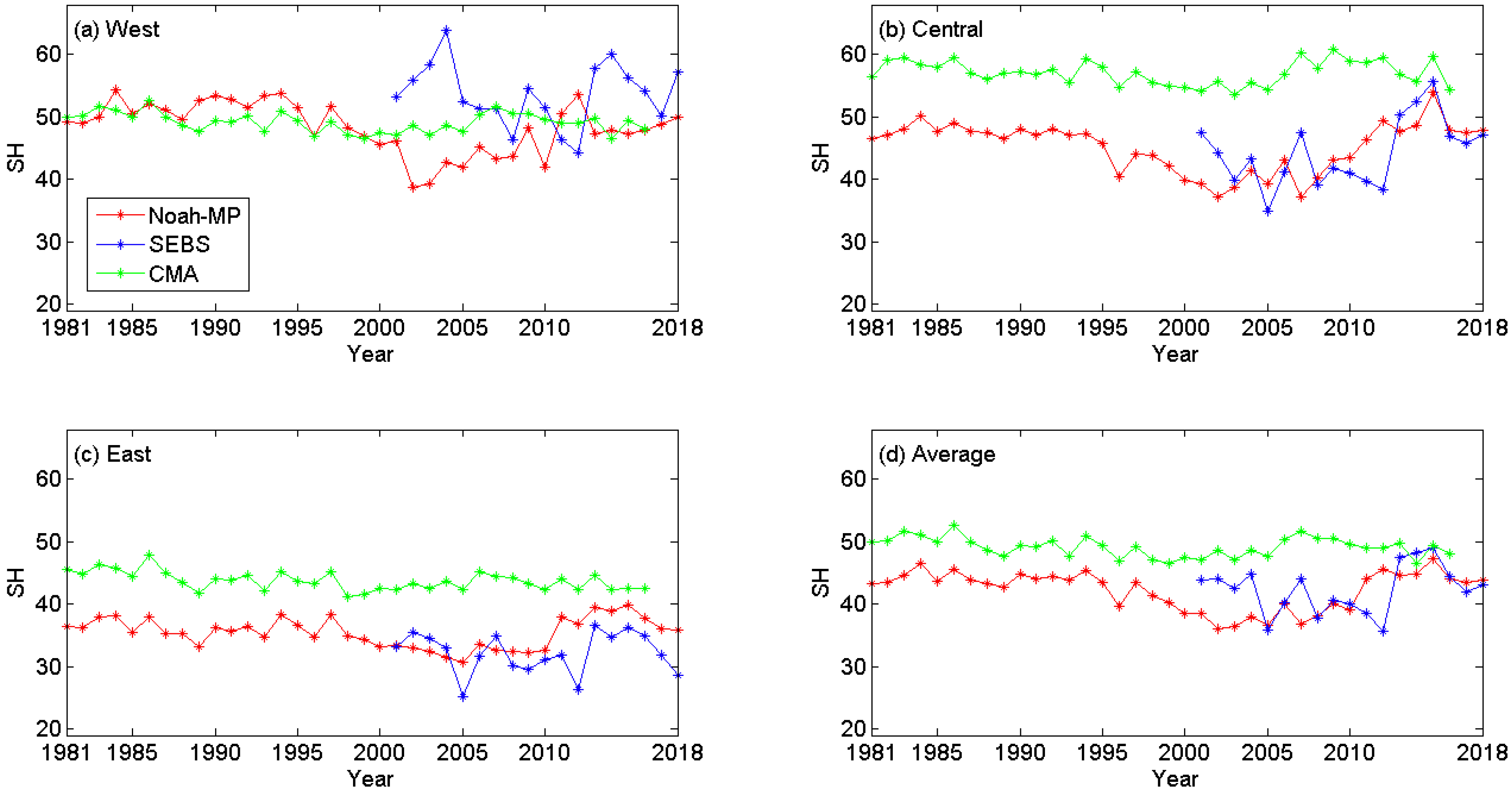
We also analyzed the annual variation trends in the SH flux over the whole TP. We divided the TP into 3 climate zones: dry western TP (west of 85°E), transitional central TP (85°E–95°E), and wet eastern TP (east of 95°E). The weather stations established by the CMA are unevenly distributed on the TP, with most located in the eastern and central regions of the TP. Figure 5 shows the annual variations in SH flux from Noah-MP, SEBS, and CMA station data for the western, central, eastern and entire TP. In the Noah-MP simulation, the SH fluxes among the 3 sub-regions and over the entire TP all exhibited significant decreasing trends beginning in the mid-1980s, as was also reported in previous studies [11,13]. These decreasing trends were more obvious on the western and central TP than on the eastern TP. However, all regions showed an increasing trend from the beginning of the 21st century, with the eastern TP experiencing the increasing trend later than the western and central TP. Overall, the decreasing trend was approximately 0.31 W m−2 per yr, while the increasing trend was 0.64 W m−2 per yr. Both the decreasing and increasing trends were more significant than those obtained from CAM station-based results. In the SEBS simulation on the western TP (Figure 5a), the annual mean SH fluxes were much stronger than those in the Noah-MP simulation, and the trend was not significant during the period 2001–2018. There was a big difference between the two simulation results during the period 2001–2004. The SH flux from SEBS showed an upward trend beginning in 2001, while Noah-MP gave an increasing trend only after a decrease in 2002. On the central TP (Figure 5b), both Noah-MP and SEBS gave an increasing trend in the annual mean SH flux. The CAM station-based SH fluxes were larger than those from the Noah-MP and SEBS simulations. On the eastern TP (Figure 5c), trends obtained from the two models were relatively consistent. Meanwhile, the annual mean SH fluxes from SEBS became weaker than those from Noah-MP from 2008 onwards. However, both Noah-MP and SEBS gave smaller values of SH flux compared with the CAM station-based results. Moreover, the CAM station-based SH fluxes began to increase earlier than those of Noah-MP and SEBS. Figure 5d shows the variations in annual mean TP-averaged SH fluxes from Noah-MP, SEBS, and CMA station data. The changes in CAM station-based SH flux were similar to the simulated results on the eastern TP (Figure 5c), because 54 of the 80 stations were installed on the eastern TP. Overall, simulated TP-averaged SH fluxes began to increase later than the CAM station-based results. Chen et al. [25] also reported similar results, showing that the reversal of trends derived from reanalysis products (ER-Interim and NCEP) happened later than for those derived from CAM station data.
3.3. Causes of the Trends
The bulk transfer coefficient method is typically used to calculate the surface SH flux. The surface wind speed, temperature difference between the ground surface and air (Ts–Ta), and heat transfer coefficient (CH) are key determinants of SH flux. Hence, Ts–Ta, wind speed, and CH were analyzed to determine the main causes of the increasing and decreasing trends in the Noah-MP simulations.
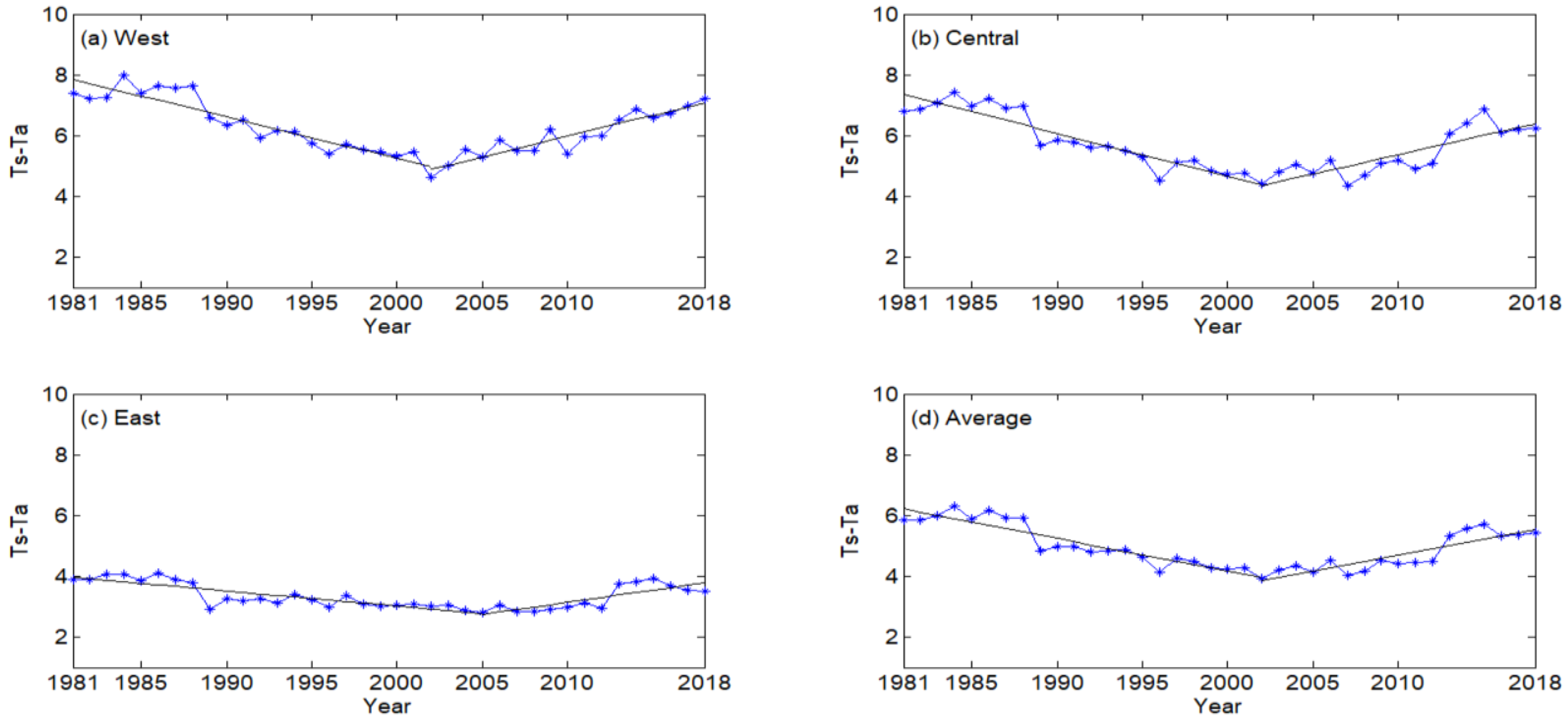
Figure 6 shows the variations in annual mean Ts–Ta in the Noah-MP simulations on the TP during the period 1981–2018. There was an obvious decreasing trend from the mid-1980s to the beginning of the 21st century on the western TP (Figure 6a). Then, the trendline turned sharply upwards. This phenomenon also existed on the central TP (Figure 6b). Figure 6c shows the annual mean values of Ts–Ta and the corresponding trends on the eastern TP. The values of Ts–Ta were smaller than those of the western and central TP. Meanwhile, both the decreasing and increasing trends were not as significant as those of the western and central TP. The TP-average trends are shown in Figure 6d. Both the decreasing trend and increasing trend were significant, similar to the trends based on Noah-MP shown in Figure 5d. The correlation coefficient between annual mean SH flux and Ts–Ta was 0.74. This conflicts with the results of Yang et al. [9], who reported an increase in Ts–Ta from approximately 1970 to 2006. However, the Ts–Ta trends reported herein agree with the results based on reanalysis products (ERA-Interim and NCEP) reported by Chen et al. [25].
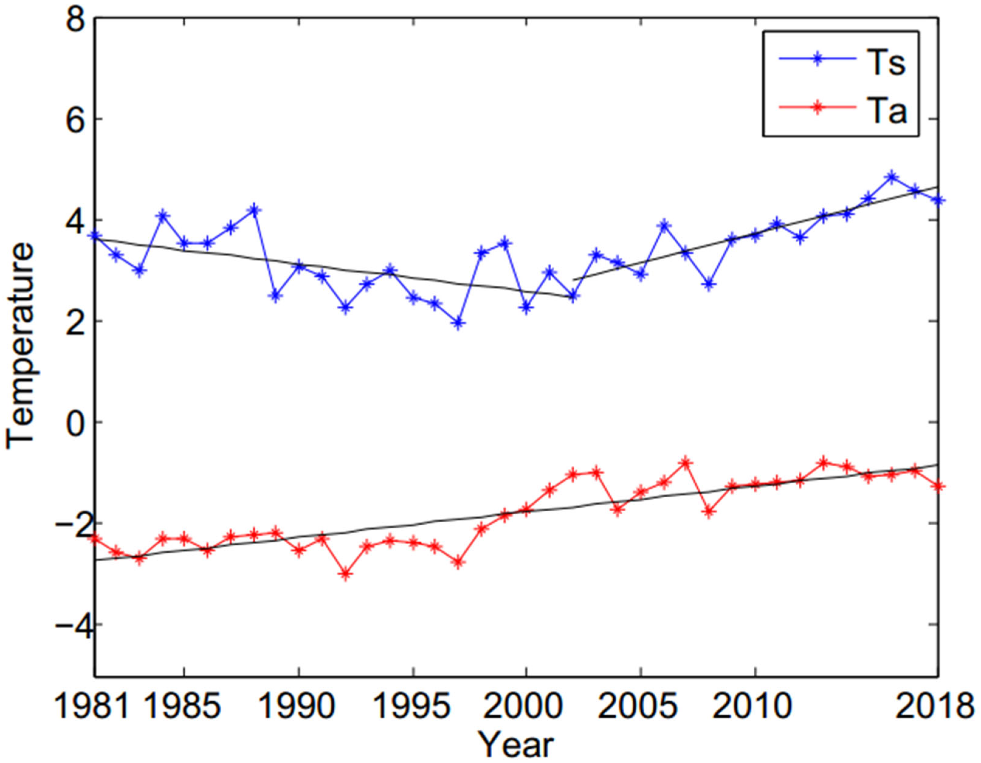
For the whole TP, the variations in Ts and Ta in the Noah-MP simulation were also calculated, and are shown in Figure 7. We found that, Ta showed an increase during the period 1981–2018. This increasing trend was also reported in previous studies [9,11]. However, Ts experienced a period of decrease before 2002; from then on, Ts also showed an increase. This shift resulted in the transition of Ts–Ta in approximately 2002. In the Noah-MP and SEBS simulations, SH fluxes began to increase later than in the CAM station-based results. The annual Ts variation trends of correlate well with those of Ts–Ta and SH flux on the TP.
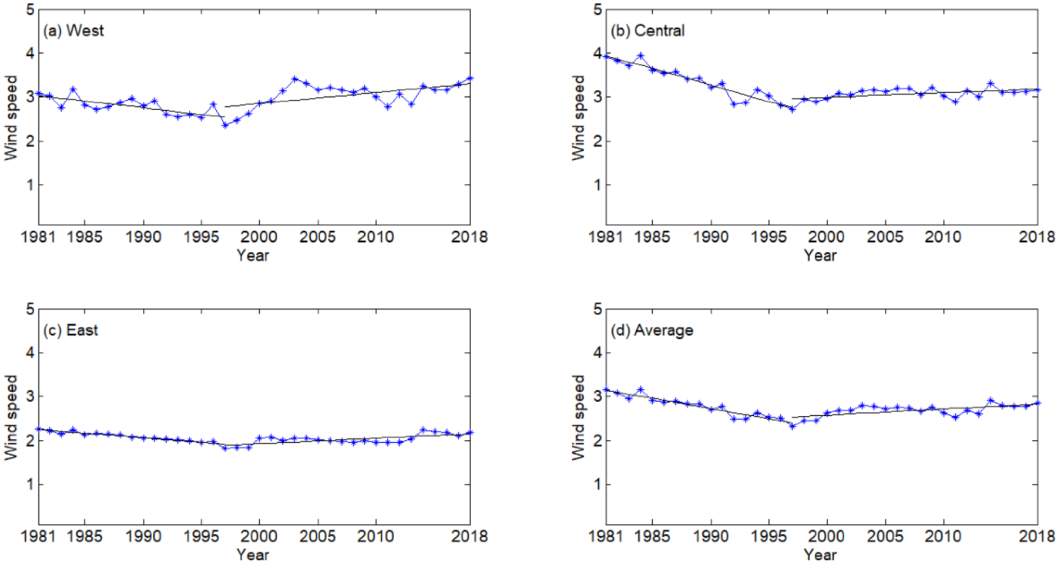
Figure 8 shows the annual variation in wind speed (10 m above the ground), which was derived from the atmospheric forcing data (CMFD). The central and western TP experienced greater wind speeds than did the eastern TP during the 38-yr study period. The values of annual mean wind speed in all the 3 sub-regions declined from the mid-1980s, and then increased from approximately 1998. However, these changes were not very clear, especially on the eastern TP. Overall, the wind speed over the TP decreased from 1981 to 1998, and then increased after 1998 (Figure 8d). The changes in wind speed contributed substantially to the SH flux before 1998. Duan et al. [11] also considered this reduction in surface wind speed was also considered to be the cause of the decrease in SH flux. Yang et al. [9] attributed the changes in surface wind speed to the downward momentum transport of upper-air wind modulated by the upper-air pressure gradient.
Nevertheless, the heat transfer coefficient CH in the Noah-MP simulations was also analyzed to determine its annual variations. However, this showed were no clear trends across the whole TP. The changes in surface wind speed and ground-air temperature gradient were the two major factors that contributed to the changes in the SH flux, as reported in previous studies [9,11]. From the analysis above, we found that surface wind speed began to increase from approximately 1998, while Ts–Ta increased sharply after 2002. During the period 1998–2002, Ts–Ta retained a decreasing trend, and this contributed to the decreasing trend in SH flux during this period. This was caused by Ts retaining a decreasing trend during this period. Overall, Ts–Ta trends were similar to those of annual mean SH flux in both Noah-MP and SEBS. Both Ts–Ta and SH flux showed a transition at the beginning of the 21st century in the Noah-MP and SEBS simulations and in the reanalysis products (ERA-Interim and NCEP) reported by Chen et al. [25].
4. Conclusions and Discussion
Decadal trends in SH flux on the TP, especially when and how the trends changed, remain controversial. Here, we analyzed the climatic features of the SH flux on the TP using the high-resolution Noah-MP and SEBS simulations, and compared these results with the CMA station-based results.
The western and central TP witnessed much larger mean SH fluxes than did the eastern TP in both the Noah-MP and SEBS simulations. Meanwhile, the inter-annual variations in SH fluxes on the central and western TP were larger than that on the eastern TP. The SEBS simulation showed much larger inter-annual variations than did the Noah-MP simulation in most areas of the TP. The Yang method [41] applied to CMA station data here produced higher SH fluxes compared with the Noah-MP and SEBS simulations. We confirmed the decreasing trend in SH flux on the TP from the mid-1980s to the beginning of the 21st century, as also reported in previous studies [11,13]. Overall, the subsequent increasing trend in SH flux began in approximately 2002. The SEBS simulation showed much stronger SH fluxes on the western TP, but weaker SH fluxes on the eastern TP during 2001–2018 compared with the Noah-MP simulation. Both the Noah-MP and SEBS simulations showed an increasing trend in the TP-averaged SH flux from the beginning of the 21st century. The CAM station-based results showed an increasing trend before 2000, earlier than that recorded by both Noah-MP and SEBS. The model-based results showed consistent trends with those obtained from reanalysis products (ERA-Interim and NCEP) reported by Chen et al. [25].
Overall, there was a close relationship between changes in mean Ts–Ta and trends in the SH flux. Annual mean Ts experienced a period of decrease period before 2002, and then increased significantly. This shift in Ts resulted in the Ts–Ta transition in approximately 2002. Hence, the changes in Ts were the main cause of the changing trends in SH flux on the TP. The central and western TP experienced greater wind speeds than did the eastern TP during the 38-yr study period. Overall, the wind speed over the TP decreased from 1981 to 1998, and then increased after 1998. This explains why SH fluxes derived from CMA station data using conventional methods showed an early transition before 2000 in previous studies [13,25,43]. The changes in wind speed after 1998 were not as important as Ts–Ta in terms of modulating the SH flux trends. During the period 1998–2002, Ts–Ta continued to decrease, and this contributed to the decreasing trend in SH flux during this period.
It should be pointed out that the wind speed derived from reanalysis products was recorded at a height of 10 m above the ground. Wind speed at 10 m has been widely used to calculate CH and SH flux based on the bulk transfer coefficient method. This may result in larger SH fluxes than compared with using the EC system. From the analysis of the Noah-MP simulation, the SH flux on the TP showed a decreasing trend from the mid-1980s, but an increasing trend since approximately 2002. The changes in mean Ts–Ta are here credited as the main cause of the decreasing and increasing trends in SH flux on the TP. The nonconformity of changes in surface wind speed and ground-air temperature gradient may result in disagreements as to the cause of SH flux trends on the TP, as highlighted by some previous studies. Additional in situ and remote sensing-based datasets are needed to clarify this issue.
Author Contributions
Conceptualization, S.W. and Y.M.; analysis, S.W. and Y.M.; investigation, S.W. and Y.L.; writing-original draft preparation, S.W.; writing-review and editing, S.W. and Y.M.; visualization, S.W. and Y.L.; supervision, Y.M. All authors have read and agreed to the published version of the manuscript.
Funding
This work was funded by the Second Tibetan Plateau Scientific Expedition and Research (STEP) program (2019QZKK0103), and the National Natural Science Foundation of China (42075156 and 91837208).
Data Availability Statement
The datasets generated and analyzed during the current study are not publicly available, but are available from the corresponding author on reasonable request.
Conflicts of Interest
The authors declare no conflict of interest.
References
- Chen, L.; Reiter, E.; Feng, Z. The atmospheric heat source over the Tibetan Plateau: May–August 1979. Mon. Weather Rev. 1985, 113, 1771–1790. [Google Scholar] [CrossRef]
- Ye, D.; Wu, G. The role of the heat source of the Tibetan Plateau in the general circulation. Meteorol. Atmos. Phys. 1998, 67, 181–198. [Google Scholar] [CrossRef]
- Wu, G.; Liu, Y.; He, B.; Bao, Q.; Duan, A.; Jin, F.-F. Thermal controls on the Asian summer monsoon. Sci. Rep. 2012, 2, 404. [Google Scholar] [CrossRef] [PubMed] [Green Version]
- Zhao, P.; Chen, L. Study on climatic features of surface turbulent heat exchange coefficients and surface thermal sources over the Qinghai-Xizang (Tibetan) Plateau. J. Meteorol. Res. 2000, 14, 13–29. [Google Scholar]
- Duan, A.; Wang, M.; Lei, Y.; Cui, Y. Trends in summer rainfall over China associated with the Tibetan Plateau sensible heat source during 1980–2008. J. Clim. 2013, 26, 261–275. [Google Scholar] [CrossRef] [Green Version]
- Duan, A.; Sun, R.; He, J. Impact of surface sensible heating over the Tibetan Plateau on the western Pacific subtropical high: A land-air-sea interaction perspective. Adv. Atmos. Sci. 2017, 34, 157–168. [Google Scholar] [CrossRef]
- Wang, Z.; Duan, A.; Wu, G. Time-lagged impact of spring sensible heat over the Tibetan Plateau on the summer rainfall anomaly in East China: Case studies using the WRF model. Clim. Dyn. 2014, 42, 2885–2898. [Google Scholar] [CrossRef]
- Yanai, M.; Li, C.; Song, Z. Seasonal heating of the Tibetan Plateau and its effects on the evolution of the Asian summer monsoon. J. Meteorol. Soc. Jpn. 1992, 70, 319–351. [Google Scholar] [CrossRef] [Green Version]
- Yang, K.; Wu, H.; Qin, J.; Lin, C.; Tang, W.; Chen, Y. Recent climate changes over the Tibetan Plateau and their impacts on energy and water cycle: A review. Glob. Planet. Chang. 2014, 112, 79–91. [Google Scholar] [CrossRef]
- Duan, A.; Wu, G. Weakening trend in the atmospheric heat source over the Tibetan Plateau during recent decades. Part I: Observations. J. Clim. 2008, 21, 3149–3164. [Google Scholar] [CrossRef] [Green Version]
- Duan, A.; Li, F.; Wang, M.; Wu, G. Persistent weakening trend in the spring sensible heat source over the Tibetan Plateau and its impact on the Asian summer monsoon. J. Clim. 2011, 24, 5671–5682. [Google Scholar] [CrossRef]
- Guo, X.; Yang, K.; Chen, Y. Weakening sensible heat source over the Tibetan Plateau revisited: Effects of the land-atmosphere thermal coupling. Theor. Appl. Climatol. 2011, 104, 1–12. [Google Scholar] [CrossRef]
- Yang, K.; Guo, X.; Wu, B. Recent trends in surface sensible heat flux on the Tibetan Plateau. Sci. China Ser. D 2011, 54, 19–28. [Google Scholar] [CrossRef]
- Zhu, X.; Liu, Y.; Wu, G. An assessment of summer sensible heat flux on the Tibetan Plateau from eight data sets. Sci. China Earth Sci. 2012, 55, 779–786. [Google Scholar] [CrossRef]
- Shi, Q.; Liang, S. Surface-sensible and latent heat fuxes over the Tibetan Plateau from ground measurements, reanalysis, and satellite data. Atmos. Chem. Phys. 2014, 14, 5659–5677. [Google Scholar] [CrossRef] [Green Version]
- Xie, J.; Yu, Y.; Li, J.; Ge, J.; Liu, C. Comparison of surface sensible and latent heat fluxes over the Tibetan Plateau from reanalysis and observations. Meteorol. Atmos. Phys. 2019, 131, 567–584. [Google Scholar] [CrossRef]
- Ma, Y.; Zhong, L.; Wang, B.; Ma, W.; Chen, X.; Li, M. Determination of land surface heat fluxes over heterogeneous landscape of the Tibetan Plateau by using the MODIS and in situ data. Atmos. Chem. Phys. 2011, 11, 10461–10469. [Google Scholar] [CrossRef] [Green Version]
- Ma, Y.; Wang, B.; Zhong, L.; Ma, W. The regional surface heating field over the heterogeneous landscape of the Tibetan Plateau using MODIS and in-situ data. Adv. Atmos. Sci. 2012, 29, 47–53. [Google Scholar] [CrossRef]
- Ge, N.; Zhong, L.; Ma, Y.; Cheng, M.; Wang, X.; Zou, M.; Huang, Z. Estimation of land surface heat fluxes based on Landsat 7 ETM+ data and field measurements over the northern Tibetan Plateau. Remote Sens. 2019, 11, 2899. [Google Scholar] [CrossRef] [Green Version]
- Ma, W.; Ma, Y. Modeling the influence of land surface flux on the regional climate of the Tibetan Plateau. Theor. Appl. Climatol. 2016, 125, 45–52. [Google Scholar] [CrossRef]
- Wang, S.; Ma, Y. On the simulation of sensible heat flux over the Tibetan Plateau using different thermal roughness length parameterization schemes. Theor. Appl. Climatol. 2019, 137, 1883–1893. [Google Scholar] [CrossRef]
- Zhu, L.; Huang, G.; Fan, G.; Qu, X.; Zhao, G.; Hua, W. Evolution of surface sensible heat over the Tibetan Plateau under the recent global warming hiatus. Adv. Atmos. Sci. 2017, 34, 1249–1262. [Google Scholar] [CrossRef]
- Zhang, C.; Tian, R.; Mao, H.; Zhang, Z.-F.; Shen, Z.-W. Temporal and spatial variation of surface sensitive heat fluxes over the middle and eastern Tibetan Plateau. Adv. Clim. Chang. Res. 2018, 14, 127–136. [Google Scholar]
- Wang, M.; Wang, J.; Chen, D.; Duan, A.; Liu, Y.; Zhou, S.; Guo, D.; Wang, H.; Ju, W. Recent recovery of the boreal spring sensible heating over the Tibetan Plateau will continue in CMIP6 future projections. Environ. Res. Lett. 2019, 14, 124066. [Google Scholar] [CrossRef] [Green Version]
- Chen, L.; Pryor, S.C.; Wang, H.; Zhang, R. Distribution and variation of the surface sensible heat flux over the central and eastern Tibetan Plateau: Comparison on of station observations and multireanalysis products. J. Geophys. Res. Atmos. 2019, 124, 6191–6206. [Google Scholar] [CrossRef]
- Li, M.; Babel, W.; Chen, X.; Zhang, L.; Sun, F.; Wang, B.; Ma, Y.; Hu, Z.; Foken, T. A 3-year dataset of sensible and latent heat fluxes from the Tibetan Plateau derived using eddy covariance measurements. Theor. Appl. Climatol. 2015, 122, 457–469. [Google Scholar] [CrossRef] [Green Version]
- Ma, Y.; Hu, Z.; Xie, Z.; Ma, W.; Wang, B.; Chen, X.; Li, M.; Zhong, L.; Sun, F.; Gu, L.; et al. A long-term (2005–2016) dataset of hourly integrated land-atmosphere interaction observations on the Tibetan Plateau. Earth Syst. Sci. Data 2020, 12, 2937–2957. [Google Scholar] [CrossRef]
- Mauder, M.; Foken, T. Documentation and Instruction Manual of the Eddy Covariance Software Package TK3; Work Report; University of Bayreuth: Bayreuth, Germany, 2011. [Google Scholar]
- Niu, G.; Yang, Z.; Mitchell, K.E.; Chen, F.; Ek, M.B.; Barlage, M.; Kumar, A.; Manning, K.; Niyogi, D.; Rosero, E.; et al. The community Noah land surface model with multiple parameterization options (Noah-MP): 1. Model description and evaluation with local-scale measurements. J. Geophys. Res. 2011, 16, D12109. [Google Scholar] [CrossRef] [Green Version]
- Yang, Z.; Niu, G.; Mitchell, K.E.; Chen, F.; Ek, M.B.; Barlage, M.; Longuevergne, L.; Manning, K.; Niyogi, D.; Tewari, M.; et al. The community Noah land surface model with multiple parameterization options (Noah-MP): 2. Evaluation over global river basins. J. Geophys. Res. 2011, 116, D12110. [Google Scholar] [CrossRef]
- Gao, Y.; Li, K.; Chen, F.; Jiang, Y.; Lu, C. Assessing and improving Noah-MP land model simulations for the central Tibetan Plateau. J. Geophys. Res. Atmos. 2015, 120, 9258–9278. [Google Scholar] [CrossRef]
- Zhang, G.; Chen, F.; Chen, Y.; Li, J.; Peng, X. Evaluation of Noah-MP Land-Model Uncertainties over Sparsely Vegetated Sites on the Tibet Plateau. Atmosphere 2020, 11, 458. [Google Scholar] [CrossRef]
- Zeng, X.; Dickinson, R.E. Effect of surface sublayer on surface skin temperature and fluxes. J. Clim. 1998, 11, 537–550. [Google Scholar] [CrossRef]
- He, J.; Yang, K.; Tang, W.; Lu, H.; Qin, J.; Chen, Y.; Li, X. The first high-resolution meteorological forcing dataset for land process studies over China. Sci. Data 2020, 7, 25. [Google Scholar] [CrossRef] [PubMed] [Green Version]
- Su, Z. The surface energy balance system (SEBS) for estimation of turbulent heat fluxes. Hydrol. Earth Syst. Sci. 2002, 6, 85–100. [Google Scholar] [CrossRef]
- Chen, X.; Su, Z.; Ma, Y.; Liu, S.; Yu, Q.; Xu, Z. Development of a 10-year (2001–2010) 0.1° data set of land-surface energy balance for mainland China. Atmos. Chem. Phys. 2014, 14, 13097–13117. [Google Scholar] [CrossRef] [Green Version]
- Han, C.; Ma, Y.; Su, Z.; Chen, X.; Zhang, L.; Li, M.; Sun, F. Estimates of effective aerodynamic roughness length over mountainous areas of the Tibetan Plateau. Q. J. R. Meteorol. Soc. 2015, 141, 1457–1465. [Google Scholar] [CrossRef]
- Han, C.; Ma, Y.; Chen, X.; Su, Z. Trends of land surface heat fluxes on the Tibetan Plateau from 2001 to 2012. Int. J. Climatol. 2017, 37, 4757–4767. [Google Scholar] [CrossRef]
- Han, C.; Ma, Y.; Wang, B.; Zhong, L.; Ma, W.; Chen, X.; Su, Z. Long-term variations in actual evapotranspiration over the Tibetan Plateau. Earth Syst. Sci. Data 2021, 13, 3513–3524. [Google Scholar] [CrossRef]
- Duan, A.; Liu, S.; Zhao, Y.; Gao, K.; Hu, W. Atmospheric heat source/sink dataset over the Tibetan Plateau based on satellite and routine meteorological observations. Big Earth Data 2018, 2, 11. [Google Scholar] [CrossRef] [Green Version]
- Yang, K.; Qin, J.; Guo, X.; Zhou, D.; Ma, Y. Method development for estimating sensible heat flux over the Tibetan Plateau from CMA data. J. Appl. Meteorol. Clim. 2009, 48, 2474–2486. [Google Scholar] [CrossRef]
- Chen, F.; Zhang, Y. On the coupling strength between the land surface and the atmosphere: From viewpoint of surface exchange coefficients. Geophys. Res. Lett. 2009, 36, L10404. [Google Scholar] [CrossRef] [Green Version]
- Wang, H.; Hu, Z.; Li, D.; Dai, Y. Estimation of the surface heat transfer coefficient over the east-central Tibetan Plateau using satellite remote sensing and field observation data. Theor. Appl. Climatol. 2019, 108, 169–183. [Google Scholar] [CrossRef]
- Wang, H.; Zhang, J.; Chen, L.; Li, D. Relationship between summer extreme precipitation anomaly in Central Asia and surface sensible heat variation on the Central-Eastern Tibetan Plateau. Clim. Dyn. 2022, 59, 685–700. [Google Scholar] [CrossRef]
Figure 1.
Locations of the three EC stations (yellow dots) and 80 CMA stations (red dots) on the TP.
Figure 1.
Locations of the three EC stations (yellow dots) and 80 CMA stations (red dots) on the TP.

Figure 2.
Comparison of simulated and observed monthly mean SH fluxes (Wm−2) at the QOMS station (a), Nam CO station (b), and Ali station (c). The green line is the best-fit line.
Figure 2.
Comparison of simulated and observed monthly mean SH fluxes (Wm−2) at the QOMS station (a), Nam CO station (b), and Ali station (c). The green line is the best-fit line.

Figure 3.
Annual mean SH fluxes (Wm−2) simulated by (a) Noah-MP and (b) SEBS on the TP during the period 2001–2018.
Figure 3.
Annual mean SH fluxes (Wm−2) simulated by (a) Noah-MP and (b) SEBS on the TP during the period 2001–2018.

Figure 4.
Standard deviation (STD) of annual mean SH fluxes (Wm−2) simulated by (a) Noah-MP and (b) SEBS on the TP during the period 2001–2018.
Figure 4.
Standard deviation (STD) of annual mean SH fluxes (Wm−2) simulated by (a) Noah-MP and (b) SEBS on the TP during the period 2001–2018.

Figure 5.
Variations in annual mean SH flux (Wm−2) from Noah-MP, SEBS, and CMA data for the western (a), central (b), eastern (c), and entire TP (d) during the period 1981–2018.
Figure 5.
Variations in annual mean SH flux (Wm−2) from Noah-MP, SEBS, and CMA data for the western (a), central (b), eastern (c), and entire TP (d) during the period 1981–2018.

Figure 6.
Variations in annual Ts–Ta (°C) in the Noah-MP simulation for the western (a), central (b), eastern (c), and entire TP (d) during the period 1981–2018. All of the trends are derived from linear least–squares regressions and are significant at the 95% confidence level using the Mann–Kendall trend test.

Figure 7.
Variations in annual Ts (°C) and Ta (°C) in the Noah-MP simulation for the entire TP during the period 1981–2018. All of the trends are derived from linear least–squares regressions and are significant at the 95% confidence level using the Mann–Kendall trend test.
Figure 7.
Variations in annual Ts (°C) and Ta (°C) in the Noah-MP simulation for the entire TP during the period 1981–2018. All of the trends are derived from linear least–squares regressions and are significant at the 95% confidence level using the Mann–Kendall trend test.

Figure 8.
Variations in annual mean wind speed (m/s) derived from CMFD reanalysis data for the western (a), central (b), eastern (c), and entire TP (d) during the period 1981–2018. All of the trends are derived from linear least−squares regressions and are significant at the 95% confidence level using the Mann–Kendall trend test.


Table 1.
Details of the three EC systems and observation periods.
| Station | Location | Land Use | Sonic Anemometer | Period (yr) |
|---|---|---|---|---|
| QOMS | 28.21°N, 86.95°E | Bare soil | CSAT3 | 2011–2015 |
| Nam Co | 30.77°N, 90.98°E | Alpine steppe | CSAT3 | 2011–2015 |
| Ali | 33.39°N, 79.70°E | Desert | CSAT3 | 2011–2015 |
Table 2.
Parameterization schemes for the key processes in the Noah-MP model.
| Process | Scheme |
|---|---|
| Runoff | SIMGM |
| β-factor | Noah |
| Snow surface albedo | BATS |
| Stomatal resistance | Ball-Berry |
| Frozen soil permeability | Koren99 |
Table 3.
Input datasets for the SEBS model. MOD11C3 is the short name of the MODIS/Terra land surface temperature and emissivity monthly L3 global products, MOD09CMG is the short name of the MODIS/Terra surface reflectance daily L3 global products, MOD13C2 is the short name of the MODIS/Terra vegetation indices’ monthly L3 global products, GLAS stands for the Geoscience Laser Altimeter System, and SPOT stands for the Systeme pour l’Observation de la Terre sensor.
| Variables | Data Source | Data Period | Temporal Resolution | Spatial Resolution |
|---|---|---|---|---|
| Downward shortwave | CMFD | 2001–2018 | 3 h | 0.1° |
| Downward longwave | CMFD | 2001–2018 | 3 h | 0.1° |
| Air temperature | CMFD | 2001–2018 | 3 h | 0.1° |
| Specific humidity | CMFD | 2001–2018 | 3 h | 0.1° |
| Wind speed | CMFD | 2001–2018 | 3 h | 0.1° |
| Land surface temperature | MOD11C3 | 2001–2018 | Monthly | 0.05° |
| Land surface emissivity | MOD11C3 | 2001–2018 | Monthly | 0.05° |
| Height of canopy | GLAS and SPOT | 2001–2018 | Monthly | 0.01° |
| Albedo | MOD09CMG | 2001–2018 | Daily | 0.05° |
| NDVI | MOD13C2 | 2001–2018 | Monthly | 0.05° |
Disclaimer/Publisher’s Note: The statements, opinions and data contained in all publications are solely those of the individual author(s) and contributor(s) and not of MDPI and/or the editor(s). MDPI and/or the editor(s) disclaim responsibility for any injury to people or property resulting from any ideas, methods, instructions or products referred to in the content. |
© 2023 by the authors. Licensee MDPI, Basel, Switzerland. This article is an open access article distributed under the terms and conditions of the Creative Commons Attribution (CC BY) license (https://creativecommons.org/licenses/by/4.0/).
Share and Cite
MDPI and ACS Style
Wang, S.; Ma, Y.; Liu, Y. Simulated Trends in Land Surface Sensible Heat Flux on the Tibetan Plateau in Recent Decades. Remote Sens. 2023, 15, 714. https://doi.org/10.3390/rs15030714
AMA Style
Wang S, Ma Y, Liu Y. Simulated Trends in Land Surface Sensible Heat Flux on the Tibetan Plateau in Recent Decades. Remote Sensing. 2023; 15(3):714. https://doi.org/10.3390/rs15030714
Chicago/Turabian StyleWang, Shuzhou, Yaoming Ma, and Yuxin Liu. 2023. "Simulated Trends in Land Surface Sensible Heat Flux on the Tibetan Plateau in Recent Decades" Remote Sensing 15, no. 3: 714. https://doi.org/10.3390/rs15030714
Note that from the first issue of 2016, this journal uses article numbers instead of page numbers. See further details here.