
Prediction of Grassland Biodiversity Using Measures of Spectral Variance: A Meta-Analytical Review

1
Department of Geography and Environmental, University of Reading, Reading RG6 6AH, UK
2
UK Centre for Ecology and Hydrology, Wallingford OX10 8BB, UK
*
Author to whom correspondence should be addressed.
Remote Sens. 2023, 15(3), 668; https://doi.org/10.3390/rs15030668
Submission received: 30 November 2022
/
Revised: 18 January 2023
/
Accepted: 19 January 2023
/
Published: 23 January 2023
(This article belongs to the Section Ecological Remote Sensing)
Abstract
:Over the last 20 years, there has been a surge of interest in the use of reflectance data collected using satellites and aerial vehicles to monitor vegetation diversity. One methodological option to monitor these systems involves developing empirical relationships between spectral heterogeneity in space (spectral variation) and plant or habitat diversity. This approach is commonly termed the ‘Spectral Variation Hypothesis’. Although increasingly used, it is controversial and can be unreliable in some contexts. Here, we review the literature and apply three-level meta-analytical models to assess the test results of the hypothesis across studies using several moderating variables relating to the botanical and spectral sampling strategies and the types of sites evaluated. We focus on the literature relating to grasslands, which are less well studied compared to forests and are likely to require separate treatments due to their dynamic phenology and the taxonomic complexity of their canopies on a small scale. Across studies, the results suggest an overall positive relationship between spectral variation and species diversity (mean correlation coefficient = 0.36). However, high levels of both within-study and between-study heterogeneity were found. Whether data was collected at the leaf or canopy level had the most impact on the mean effect size, with leaf-level studies displaying a stronger relationship compared to canopy-level studies. We highlight the challenges facing the synthesis of these kinds of experiments, the lack of studies carried out in arid or tropical systems and the need for scalable, multitemporal assessments to resolve the controversy in this field.
1. Introduction
Grasslands are ecologically important systems, as they cover around 30–40% of the global terrestrial land mass [1], contain high levels of biodiversity [2] and provide multiple ecosystem services [3]. However, much of our global grassland resource is undergoing, or is at risk of, degradation [4] due to changes in management intensity [5,6], climate [7,8] and eutrophication [9]. To prevent further decline and ensure successful restoration, government agencies and research bodies require reliable, quantitative data on the changing status of the plant biodiversity within these systems, and remote sensing could be part of the solution [10,11].
Although most remote sensing studies aimed at vegetation monitoring are focused on forests of late, grasslands have also received more attention [12,13,14]. Herbaceous plants, which dominate grasslands, are often magnitudes smaller than their counterparts in woody vegetation, and this has been a major obstacle to applying remote sensing at the plant or leaf level. Some grasslands are dominated by a few species that can be mapped using satellite-mounted sensors [15,16]; however, natural or semi-natural grasslands are often characterized by a high community complexity within small areas [17]. In addition, grasslands are particularly dynamic over time due to variations in water availability [18] and other environmental factors. Despite these challenges, recent technological developments have made applications involving grasslands more feasible. There are now satellite missions providing small pixel sizes (10 m Sentinel-2), and high temporal resolutions (daily 250 m MODIS or every 5 days for Sentinel-2) [19] and fast-developing sensors on Unmanned Aerial Vehicles are enabling observations at very high spatial and spectral resolutions [20,21]. Some researchers have also employed proximal field instrumentation such as tram-mounted sensors [22] to obtain extremely detailed spectral information.
One attractive approach to monitoring grassland diversity, due to its simple concept, is to utilize the ‘Spectral Variation Hypothesis’ [23], which assumes that the spectral variation in space is correlated with the plant or habitat diversity. Plant diversity mapping using this method is based on the premise that individual species or plant communities have a distinct spectral reflectance signature, a product of optically detectable leaf and/or canopy traits [24]. At very small spatial scales, leaf-level optical properties drive the variance in reflectance, whereas, at larger scales, the canopy properties will be the main drivers. These relationships are well understood for single-species scenarios [25,26] but are likely to be more complex in taxonomically diverse communities.
Although the Spectral Variation Hypothesis is widely recommended and examined, the theory is not without critics [27]. It can be unstable in space (see [28], who used the approach across European landscapes) and temporally unstable interannually [29] and over growing seasons [30]. Plant materials at the leaf level are plastic, reacting to the environment in diverse ways [31,32]. The extent of plasticity in optical traits is thought to be, in part, genetically based, meaning that the taxonomic component of communities is influential [19] but not necessarily easy to predict across space and time. The approach to biodiversity monitoring at the community type level could also be problematic when applied to grasslands. For example, at these scales, grassland plants may display convergent canopy-level traits due to weather parameters, such as increases in greenness and biomass due to increased precipitation [33]. In addition, the spectral variation of grassland fields is strongly influenced by management events such as mowing and grazing [34,35].
The motivations behind applying the Spectral Variation Hypothesis display some cohesion; however, the spatial scale, instrumentation and spectral resolution of the studies vary considerably. These experimental choices could explain some of the inconsistency in the results as follows. Our ability to map taxonomic units using reflectance data is thought to be dependent on small variations that can only be detected using hyperspectral resolution data [36,37]. The Spectral Variation Hypothesis applied at the leaf level could therefore produce much weaker predictions when multi-spectral data are used. The spectral variation can be influenced by instrumentation. For example, in close range imaging spectroscopy situations, surface leaf reflectance can potentially have a large impact on spectral variance [38]. The number of taxonomic units being examined may matter, as there is evidence that the spectral variation–species diversity relationship is saturated with more complex communities [39]. The timing of sampling campaigns is also critical, as plant traits change seasonally [40,41] and interannually [42], affecting the plant spectral reflectance [43]. This is likely to have an impact on the temporal stability of the spectral variation–biodiversity relationship [44].
There have been several review papers published on the usefulness of remote sensing to assess biodiversity [45,46,47,48,49,50,51], and some have specifically looked at the Spectral Variation Hypothesis [27,52]. However, these approaches are somewhat subjective and non-standardized. A better alternative is to use a quantitative synthesis, known as a meta-analysis. Here, it is possible to weigh differences between study outcomes using the sampling effort and to investigate the impact of proposed moderating variables [53]. The method has been previously used in ecology [54,55] and in optical remote sensing to evaluate the literature relating to, for example, plant pigment concentrations [56], functional traits [57], forestry variables [58], crop variables [59] and land cover classification [60].
Here, we carry out a literature search and meta-analysis of studies that used optical remote sensing to estimate the biodiversity of grasslands under the Spectral Variation Hypothesis, with an emphasis on the effect of the spatial, temporal and spectral resolutions of the remote sensing data used, alongside other features of the sampling campaigns.
2. Materials and Methods
2.1. Literature Search and Selection of Studies for Meta-Analysis
In April 2020 and May 2022, we carried out literature searches using Google Scholar and Scopus (Table S1) following the PRISMA (Preferred Reporting Items for Systematic reviews and Meta-analysis) methodology [61]. We read paper abstracts to ascertain whether studies contained spectral data and dealt with plant biodiversity in grassland systems. We did not include studies that mapped specific taxonomic units or that aimed to differentiate between a small number of target species. Some of the searches produced a very large number of records. In these cases, after sifting through 100 pages of results, (of approximately 10 results per page), the search was abandoned. The initial searches produced 74 papers, with an extra 4 found through reference lists, giving a total of 78 papers. These were then examined in more detail, and duplicates were removed, giving 77 studies. These were included in the final data set if the authors:
- Explicitly tested whether plant species richness or diversity was correlated with a measure of spectral variance in space.
- Included a Pearson’s Correlation Coefficient that resulted from a bivariate model or an r2 value with an indication of the relationship direction.
- Did not deal with environments such as in savannahs or mixed planned countryside.
This left 20 studies suitable for our quantitative synthesis. Figure S1 provides details of the selection in the PRISMA graphical format.
2.2. Extraction and Description of Likely Moderators
We extracted several moderating variables that are likely to affect the relationship between spectral variance and plant species diversity. These moderators related to (1) the spectral data, (2) the species data and (3) the sampling design.
2.2.1. Spectral Moderators
We identified five moderating variables relating to the spectral data. The ground sampling size of the instrument is essential to understand if the Spectral Variation Hypothesis was tested at the leaf level or at the community/habitat level. A continuous variable in meters was created called the ‘pixel size’. In addition, a categorical variable called ‘leaf–canopy’ was generated that classified effect sizes according to whether the pixel size matched ‘leaf’- or ‘canopy’-scale measurements.
Next, we created a category called ‘spectral region’ to note the spectral region used. Here, we refer to the visible part of the spectrum as 400–699 nm, the NIR as 700–1299 nm and the SWIR as 1300–2519 nm. Since the variation within each of these spectral regions is broadly driven by differing optical leaf and canopy properties, we can use the results of this analysis to propose biochemical reasons for the link between spectral variation and species diversity. In addition, to understand if a better spectral resolution improves predictions, effect sizes were categorized as to whether they were calculated using hyperspectral or multi-spectral data under the moderator ‘spectral resolution’.
Measures of spectral variation are calculated in different ways. Some authors select a simple dispersion around the mean reflectance value, such as the range, standard deviation or the coefficient of variation, whereas others take more complex approaches, such as the average spectral angle between species [62], spectral entropy [63] or species spectral clustering measures [64]. To test whether there was an advantage in using these more complex measures, we created a variable called the ‘spectral diversity metric’, where measures were coded as either ‘simple’ or ‘complex’.
2.2.2. Species Moderators
We identified three moderating variables related to the species data. Species counts in space, also referred to as richness, is the basic measure in biodiversity assessments, but it does not capture the relative abundance of the taxa. The variable ‘species diversity’ was coded as either ‘richness’ or, where a metric also incorporated evenness or abundance, as ‘diversity’.
Additionally of interest is the number of species considered in the study. In grasslands, the species richness levels can be very high per m2. In previous works, it has been suggested that our ability to predict taxonomic units using spectral variance may be saturated as the number of species in a data set rises [65,66]. Therefore, effect sizes may be smaller when looking at communities where species richness is consistently high. To test this idea, the continuous moderator ‘richness level’ was created, using the minimum value of richness within an analysis, as a proxy for the taxonomic complexity of the analysis. We hypothesize that the mean effect will be negatively influenced by higher numbers of species.
The methods of assessing biodiversity are classified according to the scale of organization, known as alpha, beta or gamma diversity [67]. Alpha is the number of species within a unit area and can also include a measure of their relative abundance. Beta diversity captures community dissimilarities between patches or components of a landscape. Gamma diversity is an additive measure of both alpha and beta diversities and describes diversity at the landscape scale. We created the categorical moderator ‘level of diversity’ to capture these different scales.
2.2.3. Sampling Design
We identified four moderating variables related to sampling design. Firstly, we noted that the sampling effort difference between the spectral and the botanical data is often pronounced. For example, satellite sensors collect spectral data over large areas, whereas the accompanying field botanical data have a much sparser coverage and are extrapolated from small plots. In contrast, when aerial or handheld instruments are used, small plots are often sampled exhaustively for both spectral and botanical data. To understand if these differences in the sampling effort impact the effect size, we created the moderator ‘spatial matching’, which is the ratio of the area sampled botanically to the area sampled spectrally.
Secondly, the time of year that sampling occurs is likely to impact the relationship between spectral variance and species diversity. Leaf and canopy phenology drive changes in reflectance over a growing season, and therefore, the relationship between spectral variance and plant diversity is also expected to vary over time. Summer should be the most stable time of the year for sampling leaf spectra. To capture this, we created a variable called ‘sampling season’. We noted the first and the last month that spectral data were collected and categorized these months into seasons as follows: ‘summer’ (June–August) or ‘other’. We recognize the somewhat arbitrary nature of these sampling periods, as seasonality will not be uniform across our sites due to the latitude and continentality of sites.
Thirdly, we used the Köppen climate classification to classify sites into one of five main groups (tropical, arid, temperate, continental and polar) according to their seasonal temperature patterns [68] in order to explore the impact of the ecological region on the reliability of the hypothesis. We called this variable ‘climate’.
Finally, the level of naturalness of systems may affect the extent to which the Spectral Variation Hypothesis works. More natural systems often have higher levels of complexity in terms of their species distribution in space. In experiments, diversity levels are manipulated through, for example, seeding or weeding. To test if this has an impact, the moderator ‘site type’ was coded with two levels: ‘natural’ and ‘experimental’.
2.3. Data Analysis
2.3.1. Extraction of Effect and Sample Sizes
To carry out a meta-analysis, we needed a standardized effect size for each result across all studies. Suitable effect sizes in studies that dealt with two continuous variables were generally based on Pearson’s Correlation Coefficients or associated values of the co-efficient of determination (r2), where additional information was available about the direction of the relationship. When results were only available as graphic displays, we extracted the estimates using the software ‘Plot Digitizer’ [69]. The results based on Kendall’s rank were converted to the Pearson’s Correlation Coefficient [70]. We transformed all estimates to Fisher’s Z [71] to improve the fit to a normal distribution. Next, we weighted them for the meta-analysis using effect-level sample sizes based on the number of sampled botanical areas (e.g., plots or fields) used in the analysis. The sampling variances were calculated using large sample approximations and bias corrected correlation coefficients [72]. Model estimates based on Fisher’s Z were converted back into the Pearson’s Correlation Coefficient for interpretation purposes.
2.3.2. Three-Level Meta-Analytical Models
One of the challenges with synthesizing outcomes of remote sensing studies is that there are often multiple results reported within one study, leading to the challenge of modelling dependence of the effect sizes. Traditionally, this problem is handled by creating a mean effect size for each study [73]. However, this discards useful information that can, for example, be used to assess the impact of moderators. A more recent approach has been to use a multi-level extension also known as a three-level model, which enables us to estimate the variance not attributable to sampling errors and to specify both the within-cluster and between-cluster variances [74]. Firstly, we specified models clustered by ‘study’, a common approach in meta-analyses. Secondly, we used ‘site’ as a clustering variable, as high levels of between-study variations could be driven by site specificity. In addition, to test if our likely moderating variables impact mean effect sizes, we evaluated their importance by carrying out a subgroup analysis within a mixed effects model framework. Due to the data set size, we first included these moderators individually, and then, if they were significant, we tested for interactions [75]. We used the restricted maximum likelihood estimator (REML) to evaluate the significance of the main effect size for each model. For the moderator models, we estimated different effect sizes for each level of the categorical moderator. If the moderator was a continuous variable, we estimated the overall effect size and tested its significance.
When each study design is identical, all variances between study effect sizes should be attributable to the sampling error (i.e., sampling effort). Outside clinical trials, this is almost never true. Especially in ecological studies, we would expect there to be high levels of variance between study results due to the high levels of variation in natural systems. In meta-analyses, ‘heterogeneity’ is used to describe variances not attributable to sampling errors. Here, we report the significance level of Cochrane’s Q for an overall test of ‘heterogeneity’ in the models, followed by I2 [76]. The I2 statistic is a relative value that indicates the percentage of total variance that is not attributable to a sampling error. It can be further decomposed into I2 level-two and I2 level-three variances, which are, respectively, the between-cluster and within-cluster variances. We tested the significance of the variance decomposition by comparing the three-level model with the equivalent two-level model using a one-sided log-likelihood-ratio test. We also evaluated the changes in the I2 value as different moderators were added to the basic model.
2.3.3. Sensitivity Analysis and Publication Bias
For each three-level model, we carried out a sensitivity analysis. Influential case diagnostics were produced using a multivariate measure analogous to Cook’s distance [77], which can be interpreted as the Mahalanobis distance between the entire set of predicted values, with the ith case included and excluded from the model fitting. These diagnostics were carried out at the study cluster level for each model. A robust cut off value for influential data does not exist, but generally, a Cook’s distance > 4/n is used, where n is the number of clusters in the model. To test if outlier studies were having a strong effect on the results, outliers were removed and the models recalculated.
Publication bias arises when results from studies are more likely to be published if they fulfil existing expectations. In the case of testing the Spectral Variation Hypothesis, this would result in finding a strong positive correlation between species or habitat diversity and spectral variance and, within the meta-analytical framework, an overestimation of the mean effect size. There are limited methods available for estimating publication bias in data sets that display dependence [78]. One simple option is to visually inspect funnel plots where residual values from the meta-analysis are plotted against the standard error. Non-symmetrical plots indicate the presence of publication bias.
3. Results
3.1. Overview of Studies
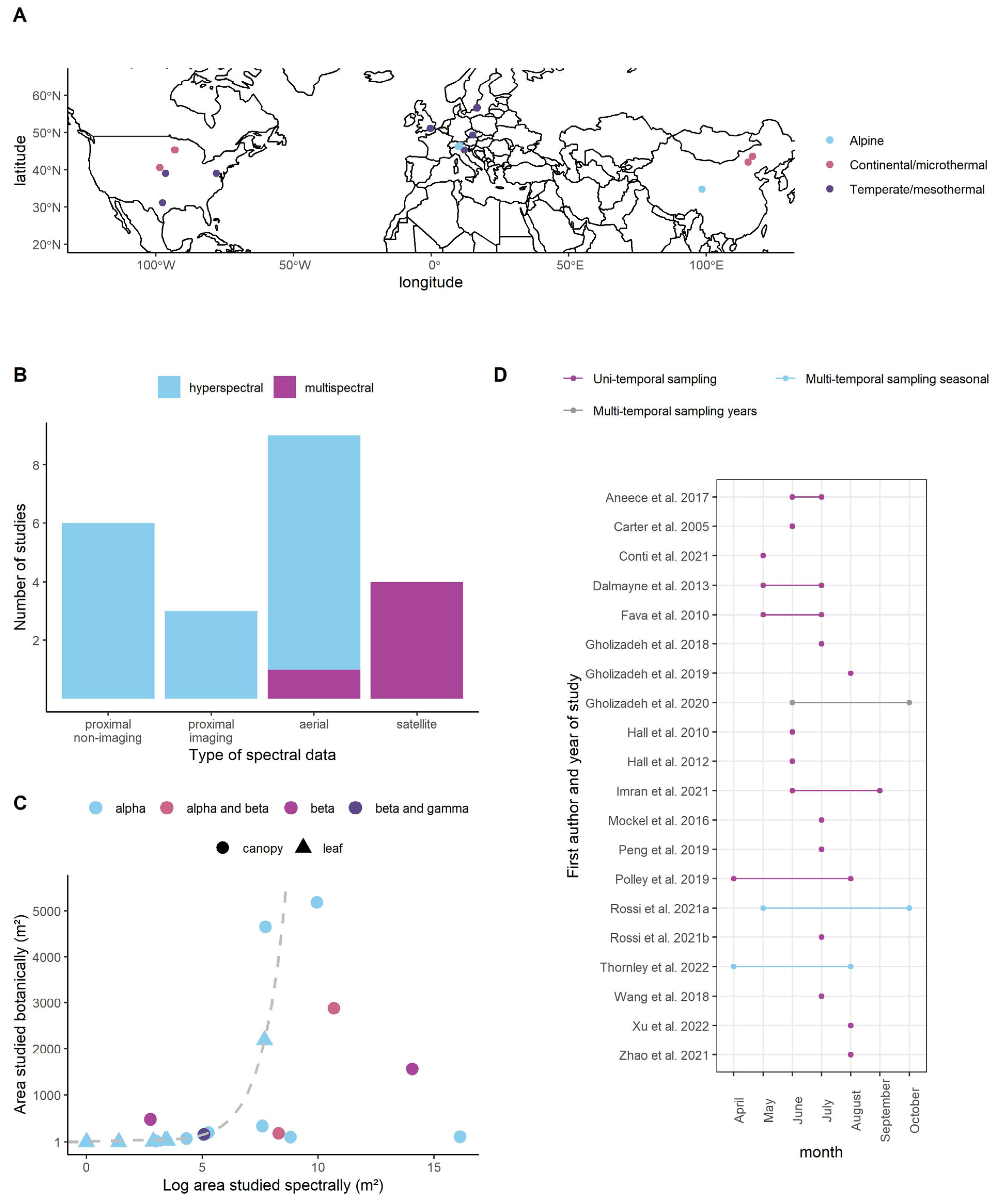
In terms of study location, there was a strong research bias towards sites in North America and Northwestern Europe. Three studies were carried out in Northern China (Figure 1A). There were no studies carried out in the Southern Hemisphere. All grasslands could be classed as temperate, continental or alpine, with no examples of tropical or arid systems. There was a good mix of leaf- and canopy-level studies, captured using satellites, unmanned aerial vehicles and proximal instruments (Figure 1B). We found studies that looked at alpha and beta diversities but only one that investigated gamma diversity (Figure 1C). The effect size for gamma diversity was excluded from future analyses due to the small sample size. Three studies collected data at discrete time points and explicitly reported results on the temporal stability of the Spectral Variation Hypothesis. Two studies did this across a growing season and one over different years. Some authors treated field data collected across a few months as a single sampling point (Figure 1D).
Most studies focused on a particular aspect of the relationship between spectral variance and biodiversity: six tested different biodiversity metrics using the same data set, four looked at the relationship at spatial different scales (i.e., pixel sizes), three looked at the relationship over time, six calculated the spectral variation in different ways and five repeated the same experiment across different sites or fields. Table 1 lists the publications, alongside their thematic focus.
3.2. Results of the Multi-Level Models
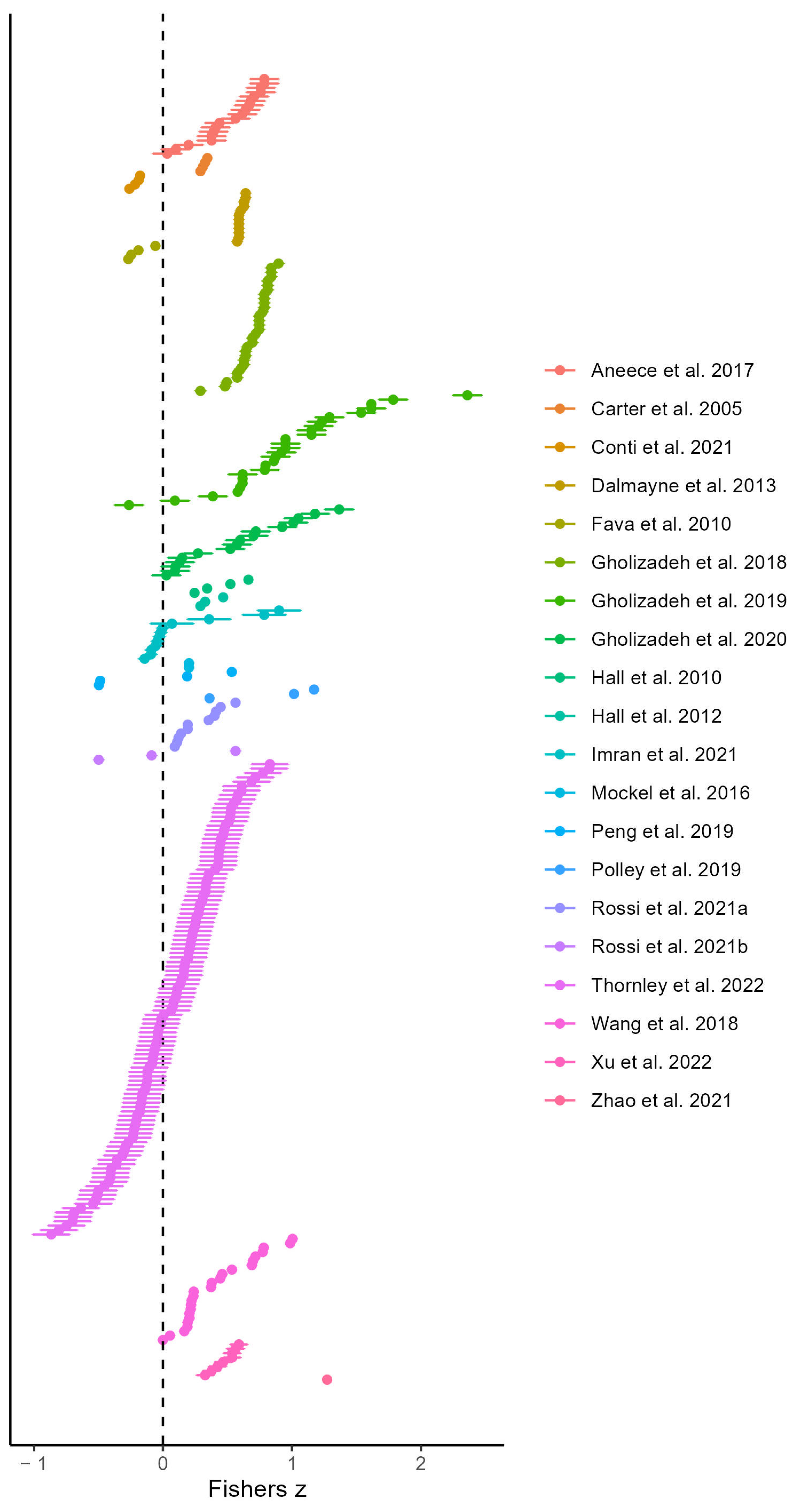
For the meta-analysis, we extracted 297 effect sizes from 20 studies over 15 experimental locations. A forest plot shows these effect sizes with their sampling variance by study category (Figure 2). The mean effect size (Pearson’s Correlation Coefficient) calculated for the basic three-level meta-analysis models (no moderators) with study or site as the clustering variable, respectively, was 0.358 or 0.32 (confidence interval ±0.161 or 0.197), suggesting that, overall, there is a positive relationship between spectral variance and plant species diversity. We tested for the significance of the variance components by comparing the three-level model with the equivalent two-level model. Both three-level models, with level three heterogeneity constrained to zero, were a better fit for the data than their equivalent two-level models at p = 6.897 × 10⁻²² (study) and p = 2.076 × 10⁻²⁰ (site) when using a likelihood-ratio test. Using the three-level approach, heterogeneity was decomposed into sampling between-cluster (level 2) and within-cluster (level 3) variances, each level being expressed as a percentage of the total model variance. The measure of heterogeneity (I2) across all models was significant and substantial at about 80%, with about two-thirds of the heterogeneity occurring within studies. The results of the variance partitioning for the three-level models was very similar, whether study or site were defined as the clusters. Therefore, going forward, we report only the models clustered by study.
Most of the moderating variables were not found to be significant, and the inclusion of moderators did not change the proportion of variance attributable to level-two and -three variances in the models. The exceptions were moderator models that included the ‘leaf–canopy’ term, where leaf-level studies were predicted to have a higher effect size (0.49 ± 0.128) compared to canopy-level studies (0.31 ± 0.146) at p = 0.0036. The continuous moderator ‘richness level’ was also significant but with a very small effect size (0. 00161) at p = 0.043. Full model results, alongside their diagnostic criteria, are provided in Table 2. We also tested for interactions between ‘leaf–canopy’ and the other moderator variables. We found significant interaction terms of ‘leaf–canopy’ and ‘sampling season’, ‘site type’ and ‘richness level’. The results of these interaction models are in Table S2.
Cook’s distance values indicated which studies were influential on the outcome of the basic and moderator models (i.e., outliers; see Figure S2). The results of the reprocessed three-level models showed that the basic model without moderators was still significant without outliers but that the mean effect size was lower at 0.32 (±0.149) (Table S3). Outlier removal did not change the significance level of the moderating variables. The only exception was the addition of ‘site type’ as significant at p = 0.0323, with the category natural sites showing a stronger relationship compared to the experimental ones (0.5 (±0.191) and 0.24 (± 0.194), respectively). Funnel plots show no significant publication bias in any of the specified models (see Figure S3 for a basic model example).
4. Discussion
4.1. The Spectral Variation Hypothesis across Studies and Moderator Impact
The positive pooled effect size across studies of +0.36 indicates that, overall, the Spectral Variation Hypothesis appears to hold in grassland systems. The sensitivity analysis showed there was a strong influence on this mean effect size by the findings of Zhao et al. 2021 [66]. This study contained the only leaf-level result where reflectance data was collected using a leaf clip as opposed to close range imaging spectroscopy instruments and contained a single correlation that was very high (0.85). This indicates that we should be cautious when scaling our inferences from the leaf clip to imaging devices, as the taxonomic component of reflectance is weaker with imaging devices due to additional variables such as the specular reflectance [38]. However, even with the removal of this study, the mean effect size was still positive and significantly different from zero (+0.33 +/−0.149) (see Table S3). The weak-to-moderate overall effect size could be due to a nonlinear relationship between spectral variation and plant species or habitat diversity. Amongst the studies examined, almost all the available results were produced when testing for a linear relationship (nonlinear relationships were only examined in one study [81]). Testing for these alternative relationships should be an avenue of future research.
We tested whether the magnitude of the effect sizes across studies depended on reflectance observations from within single spectral regions (the visible, NIR or SWIR) or across the spectrum. We proposed that certain spectral regions may be more important than others for assessing biodiversity. However, there was no evidence from the meta-analysis that this was the case, nor did models containing data sampled from across the spectrum have a stronger relationship with plant/habitat diversity. This finding is unfortunate for two reasons. Firstly, for practical applications, such as sensor design, we require a better understanding of which spectral bands matter more [97]. Secondly, understanding which optical traits are driving the spectral variation–biodiversity relationship [27], within which contexts, is important for ecological interpretation. The results from this meta-analysis support the idea that the grounds for detecting biodiversity within grasslands could be location-specific.
The only clearly significant moderating variable, at p < 0.01, was the ‘leaf–canopy’ variable. Leaf-level studies had a higher mean effect size (0.49) compared to the canopy-level studies (0.32), implying that biodiversity estimations using optical leaf traits as opposed to habitat/community heterogeneity are a distinct methodological approach. The moderator interaction term between the ‘leaf–canopy’ and ‘sampling season’ was also significant (see Table S2). There was no relationship between spectral variance and biodiversity for leaf-level studies outside the summer season, whereas, for canopy-level studies, the relationship held for non-summer sampling. This indicates that summer sampling is more critical for leaf-level than for canopy-level approaches and that the Spectral Variation Hypothesis, at the canopy scale, may be successfully used during the spring and autumn when non-mature or senescing vegetation is present. The results of the interaction model with ‘leaf–canopy’ and ‘site type’ as terms suggest that experimental sites, rather than natural grasslands, have larger effect sizes for leaf-level estimates compared to canopy-level and vice versa. At the canopy level, the effect of higher levels of species richness was very slightly positive compared to the leaf level, where there was no effect. This result does not support our hypothesis that, in data sets with high numbers of species, our ability to estimate diversity using the Spectral Variation Hypothesis decreases.
The low influence of outliers on the results of the moderator models further suggests that most of the methodological concerns associated with testing the hypothesis seem to be systematically unimportant across existing studies. The exception is perhaps the study by [30] when testing the moderating variable ‘site type’. By removing this study, the difference between the two site types (natural or experimental) became significant (but only just at p = 0.032). This study stands out, as it is the only example where repeat sampling was carried out across a season at both a natural and an experimental site.
High levels of heterogeneity were observed across all the models. This may reflect what is known in meta-analyses as the ‘apples and oranges’ effect, where we are not strictly comparing like for like [98]. High heterogeneity is, however, common in ecological meta-analyses [99], and values between 60 and 90% are usual. The high level of heterogeneity attributable to within-study variance, compared to between-study, indicates that the choice of data processing approaches within studies is responsible for more effect size variations than the study-level variables, such as site geographical location and instrumentation choice.
4.2. Limitation in the Scope of Studies
All studies included in the meta-analysis were carried out in the Northern Hemisphere. Evidence from the Southern Hemisphere and tropical and arid grasslands is notably absent. This reflects, in part, the lack of funding for experimental work in the developing world [100]. However, our exclusion of studies that dealt with partially wooded environments at the landscape scale, such as savannahs and chaparrals, impacted the scope. We predict that isolated trees in otherwise grass- and forb-dominated landscapes will probably increase the spectral diversity due to the inclusion of two very different land cover types. Other studies have shown good outcomes for the estimation of tree covers in these types of communities [101,102], and we may be able to utilize these estimates as covariates alongside the Spectral Variation Hypothesis within these systems to separate out pixels that include trees and those that capture only grassland.
An observation from this meta-analysis is that, despite the phenological dynamism of grassland systems, there are only a few instances of multitemporal testing of the hypothesis. Explicit testing of temporal stability was only examined in three cases [29,30,94], with all studies reporting instability across time when using the same instrumentation and analytical approaches. Most other studies focused on a mid-summer assessment. The results from the interaction models suggest that this is a good choice, at least when dealing with spectral data captured at the leaf level.
There are likely to be some additional sources of study bias that we were not able to explore within this meta-analysis. For example, the quality of the spectral data between and within studies due to the variability in terrain variables. Rugged terrain creates shadows that affects reflectance [103]. This could be especially problematic when assessing the hypothesis across large-scale landscapes using satellite data. However, terrain effects can also be observed within high spatial resolution data sets, collected using unmanned aerial vehicle technology. In future analyses, more attention should be given to validate reflectance data that could be affected by the terrain.
Although we did not detect any significant publication bias in this meta-analysis using funnel plots, this result should be treated with caution, as methods for testing publication bias with dependent data sets are still under development [78]. While the non-publication of negative data is a well-known phenomenon amongst scientists [104,105], within this synthesis, we found that there was a range of both negative and positive results reported, which perhaps indicates that this phenomenon is not as prevalent in this research field as in others.
4.3. Spectral Variation as a Covariate in More Complex Models
The high level of heterogeneity in the models presented in this study imply that species diversity prediction using spectral variation is likely to require the consideration of additional covariates. Within the reviewed studies, more complex relationships were examined that incorporated biomass levels [95], vertical sward complexity [83] and the proportion of the canopy at a mature phenological stage [30]. Spectral variance has also been found to be related to ecosystem productivity in grasslands [106], and spectral diversity, captured by satellites, has been shown to be principally influenced by the land cover type [107]. Combining reflectance data with structural characteristics, such as the tree height from LiDAR [108], has also proven promising in mapping species, suggesting that different types of remotely sensed variables can be combined to predict diversity.
4.4. Approaches to the Spectral Variation Hypothesis Outside This Meta-Analysis
While examining the literature on the Spectral Variation Hypothesis, we noted emerging approaches that expand on the traditional definition, which relates to the spectral variation in space. For example, some authors have looked at the spectral variance of a pixel or cluster of pixels over time [109,110,111]. This is based on the idea that plant species or community-specific responses to temperature, rainfall, day length and soil conditions can be exploited for diversity estimations. One step further is to combine temporal and spatial spectral variations into a composite measure [94]. Spectral variance has also been used to estimate plant functional diversity [112,113]. In addition, relationships have been found between phylogenetic and spectral distances among species [114]. It is evident that, as the field of biodiversity estimations from spectral data expands, these newer approaches will require scrutiny.
5. Conclusions
The results of this study indicate that there is some promise for the use of the Spectral Variation Hypothesis to estimate biodiversity in grasslands but that more work is needed before we can exploit the method with confidence. A diverse assemblage of approaches is in use by analysts, making this an exciting and active field of research. However, this also creates challenges when synthesizing results from studies. We encourage more work in extensive natural systems, especially in tropical and arid regions, and in the Southern Hemisphere. In addition, the repetition of experiments across phenological cycles and between years will also help increase our understanding of the stability of the hypothesis across time. Hyperspectral imaging sensors that capture data at very small scales and enable scaling up to the field level (while keeping all other site and analysis variables stable) are an important link in understanding the future possibilities and limitations of this approach.
Supplementary Materials
The following supporting information can be downloaded at: https://www.mdpi.com/article/10.3390/rs15030668/s1: Table S1: The search terms used in the literature search. Figure S1: The PRISMA flow chart for standardized literature reviews and synthesis. Table S2: The results of the three-level models with the interaction terms. Figure S2: The results of the outlier analysis for the three-level models displaying the Cook’s distance metric clustered at the study level. Study outliers are those studies with values above the dotted line representing 0.2. Table S3: The results of the three-level model results after removal of the outliers at the study level. Figure S3: Funnel plot for the basic three-level model with this study as a cluster, showing (A) the raw Fisher’s Z plotted against the standard error and (B) the model residuals plotted against the standard error.
Author Contributions
Conceptualization, R.H.T., A.V., K.W. and F.F.G.; methodology, R.H.T.; software, R.H.T.; validation, K.W., A.V. and F.F.G., formal analysis, R.H.T.; investigation, R.H.T.; resources, R.H.T.; data curation, R.H.T.; writing—original draft preparation, R.H.T.; writing—review and editing, A.V. and F.F.G.; visualization, R.H.T.; supervision, A.V.; project administration, R.H.T. and funding acquisition, A.V. All authors have read and agreed to the published version of the manuscript.
Funding
The PhD studentship this research was carried out under was funded by NERC (The Natural Environment Research Council), studentship grant NE/L002566/1.
Data Availability Statement
Not applicable.
Conflicts of Interest
The authors declare no conflict of interest. The funders had no role in the design of the study; in the collection, analyses or interpretation of the data; in the writing of the manuscript or in the decision to publish the results.
References
- Gibson, D.J. Ecosystem Ecology. In Grasses and Grassland Ecology; Oxford University Press: Oxford, UK, 2008. [Google Scholar]
- Veldman, J.W.; Buisson, E.; Durigan, G.; Fernandes, G.W.; Le Stradic, S.; Mahy, G.; Negreiros, D.; Overbeck, G.; Veldman, R.G.; Zaloumis, N.P.; et al. Toward an old-growth concept for grasslands, savannas, and woodlands. Front. Ecol. Environ. 2015, 13, 154–162. [Google Scholar] [CrossRef] [PubMed] [Green Version]
- Bengtsson, J.; Bullock, J.M.; Egoh, B.; Everson, C.; Everson, T.; O’Connor, T.; O’Farrell, P.J.; Smith, H.G.; Lindborg, R. Grasslands-more important for ecosystem services than you might think. Ecosphere 2019, 10, e02582. [Google Scholar] [CrossRef]
- Bardgett, R.D.; Bullock, J.M.; Lavorel, S.; Manning, P.; Schaffner, U.; Ostle, N.; Chomel, M.; Durigan, G.; Fry, E.L.; Johnson, D.; et al. Combatting global grassland degradation. Nat. Rev. Earth Environ. 2021, 2, 720–735. [Google Scholar] [CrossRef]
- Nakahama, N.; Uchida, K.; Ushimaru, A.; Isagi, Y. Timing of mowing influences genetic diversity and reproductive success in endangered semi-natural grassland plants. Agric. Ecosyst. Environ. 2016, 221, 20–27. [Google Scholar] [CrossRef] [Green Version]
- Piipponen, J.; Jalava, M.; de Leeuw, J.; Rizayeva, A.; Godde, C.; Cramer, G.; Herrero, M.; Kummu, M. Global trends in grassland carrying capacity and relative stocking density of livestock. Glob. Chang. Biol. 2022, 28, 3902–3919. [Google Scholar] [CrossRef]
- De Boeck, H.; Lemmens, C.; Gielen, B.; Bossuyt, H.; Malchair, S.; Carnol, M.; Merckx, R.; Ceulemans, R.J.; Nijs, I. Combined effects of climate warming and plant diversity loss on above- and below-ground grassland productivity. Environ. Exp. Bot. 2007, 60, 95–104. [Google Scholar] [CrossRef]
- Ma, W.; Liu, Z.; Wang, Z.; Wang, W.; Liang, C.; Tang, Y.; He, J.-S.; Fang, J. Climate change alters interannual variation of grassland aboveground productivity: Evidence from a 22-year measurement series in the Inner Mongolian grassland. J. Plant Res. 2010, 123, 509–517. [Google Scholar] [CrossRef]
- Borer, E.T.; Seabloom, E.W.; Gruner, D.S.; Harpole, W.S.; Hillebrand, H.; Lind, E.M.; Adler, P.B.; Alberti, J.; Anderson, T.M.; Bakker, J.D.; et al. Herbivores and nutrients control grassland plant diversity via light limitation. Nature 2014, 508, 517–520. [Google Scholar] [CrossRef] [Green Version]
- Nagendra, H. Using remote sensing to assess biodiversity. Int. J. Remote. Sens. 2001, 22, 2377–2400. [Google Scholar] [CrossRef]
- Turner, W.; Spector, S.; Gardiner, N.; Fladeland, M.; Sterling, E.; Steininger, M. Remote sensing for biodiversity science and conservation. Trends Ecol. Evol. 2003, 18, 306–314. [Google Scholar] [CrossRef]
- Ali, I.; Cawkwell, F.; Dwyer, E.; Barrett, B.; Green, S. Satellite remote sensing of grasslands: From observation to management. J. Plant Ecol. 2016, 9, 649–671. [Google Scholar] [CrossRef] [Green Version]
- Reinermann, S.; Asam, S.; Kuenzer, C. Remote Sensing of Grassland Production and Management—A Review. Remote. Sens. 2020, 12, 1949. [Google Scholar] [CrossRef]
- Wang, Z.; Ma, Y.; Zhang, Y.; Shang, J. Review of Remote Sensing Applications in Grassland Monitoring. Remote. Sens. 2022, 14, 2903. [Google Scholar] [CrossRef]
- Irisarri, J.G.N.; Oesterheld, M.; Verón, S.R.; Paruelo, J.M. Grass species differentiation through canopy hyperspectral reflectance. Int. J. Remote. Sens. 2009, 30, 5959–5975. [Google Scholar] [CrossRef]
- Muthoka, J.; Salakpi, E.; Ouko, E.; Yi, Z.-F.; Antonarakis, A.; Rowhani, P. Mapping Opuntia stricta in the Arid and Semi-Arid Environment of Kenya Using Sentinel-2 Imagery and Ensemble Machine Learning Classifiers. Remote. Sens. 2021, 13, 1494. [Google Scholar] [CrossRef]
- Wilson, J.B.; Peet, R.K.; Dengler, J.; Pärtel, M. Plant species richness: The world records. J. Veg. Sci. 2012, 23, 796–802. [Google Scholar] [CrossRef]
- Zelikova, T.J.; Williams, D.G.; Hoenigman, R.; Blumenthal, D.M.; Morgan, J.A.; Pendall, E. Seasonality of soil moisture mediates responses of ecosystem phenology to elevated CO 2 and warming in a semi-arid grassland. J. Ecol. 2015, 103, 1119–1130. [Google Scholar] [CrossRef] [Green Version]
- Cavender-Bares, J.; Gamon, J.A.; Hobbie, S.E.; Madritch, M.D.; Meireles, J.E.; Schweiger, A.K.; Townsend, P.A. Harnessing plant spectra to integrate the biodiversity sciences across biological and spatial scales. Am. J. Bot. 2017, 104, 966–969. [Google Scholar] [CrossRef] [Green Version]
- Gillan, J.K.; Karl, J.W.; van Leeuwen, W.J.D. Integrating drone imagery with existing rangeland monitoring programs. Environ. Monit. Assess. 2020, 192, 1–20. [Google Scholar] [CrossRef]
- Librán-Embid, F.; Klaus, F.; Tscharntke, T.; Grass, I. Unmanned aerial vehicles for biodiversity-friendly agricultural landscapes—A systematic review. Sci. Total. Environ. 2020, 732, 139204. [Google Scholar] [CrossRef]
- Wang, R.; Gamon, J.A.; Cavender-Bares, J.; Townsend, P.A.; Zygielbaum, A.I. The spatial sensitivity of the spectral diversity–biodiversity relationship: An experimental test in a prairie grassland. Ecol. Appl. 2018, 28, 541–556. [Google Scholar] [CrossRef] [PubMed] [Green Version]
- Palmer, M.W.; Earls, P.G.; Hoagland, B.W.; White, P.S.; Wohlgemuth, T. Quantitative tools for perfecting species lists. Environmetrics 2002, 13, 121–137. [Google Scholar] [CrossRef]
- Asner, G.P.; Martin, R.E. Spectranomics: Emerging science and conservation opportunities at the interface of biodiversity and remote sensing. Glob. Ecol. Conserv. 2016, 8, 212–219. [Google Scholar] [CrossRef] [Green Version]
- Jacquemoud, S.; Baret, F. PROSPECT: A model of leaf optical properties spectra. Remote. Sens. Environ. 1990, 34, 75–91. [Google Scholar] [CrossRef]
- Jacquemoud, S.; Verhoef, W.; Baret, F.; Bacour, C.; Zarco-Tejada, P.J.; Asner, G.P.; François, C.; Ustin, S.L. PROSPECT + SAIL models: A review of use for vegetation characterization. Remote Sens. Environ. 2009, 113 (Suppl. S1), S56–S66. [Google Scholar] [CrossRef]
- Fassnacht, F.E.; Müllerová, J.; Conti, L.; Malavasi, M.; Schmidtlein, S. About the link between biodiversity and spectral variation. Appl. Veg. Sci. 2022, 25, e12643. [Google Scholar] [CrossRef]
- Schmidtlein, S.; Fassnacht, F.E. The spectral variability hypothesis does not hold across landscapes. Remote. Sens. Environ. 2017, 192, 114–125. [Google Scholar] [CrossRef] [Green Version]
- Gholizadeh, H.; Gamon, J.A.; Helzer, C.J.; Cavender-Bares, J. Multi-temporal assessment of grassland α- and β-diversity using hyperspectral imaging. Ecol. Appl. 2020, 30, e02145. [Google Scholar] [CrossRef]
- Thornley, R.; Gerard, F.F.; White, K.; Verhoef, A. Intra-annual taxonomic and phenological drivers of spectral variance in grasslands. Remote. Sens. Environ. 2022, 271, 112908. [Google Scholar] [CrossRef]
- Fritz, M.A.; Rosa, S.; Sicard, A. Mechanisms Underlying the Environmentally Induced Plasticity of Leaf Morphology. Front. Genet. 2018, 9, 1–25,. [Google Scholar] [CrossRef]
- Wu, J.; Chavana-Bryant, C.; Prohaska, N.; Serbin, S.P.; Guan, K.; Albert, L.P.; Yang, X.; van Leeuwen, W.J.D.; Garnello, A.J.; Martins, G.; et al. Convergence in relationships between leaf traits, spectra and age across diverse canopy environments and two contrasting tropical forests. New Phytol. 2016, 214, 1033–1048. [Google Scholar] [CrossRef] [Green Version]
- Cleland, E.E.; Chiariello, N.R.; Loarie, S.R.; Mooney, H.A.; Field, C.B. Diverse responses of phenology to global changes in a grassland ecosystem. Proc. Natl. Acad. Sci. USA 2006, 103, 13740–13744. [Google Scholar] [CrossRef] [Green Version]
- Bastin, G.; Scarth, P.; Chewings, V.; Sparrow, A.; Denham, R.; Schmidt, M.; O’Reagain, P.; Shepherd, R.; Abbott, B. Separating grazing and rainfall effects at regional scale using remote sensing imagery: A dynamic reference-cover method. Remote. Sens. Environ. 2012, 121, 443–457. [Google Scholar] [CrossRef]
- Giménez, M.G.; de Jong, R.; Della Peruta, R.; Keller, A.; Schaepman, M.E. Determination of grassland use intensity based on multi-temporal remote sensing data and ecological indicators. Remote. Sens. Environ. 2017, 198, 126–139. [Google Scholar] [CrossRef]
- Andrew, M.E.; Ustin, S.L. The role of environmental context in mapping invasive plants with hyperspectral image data. Remote. Sens. Environ. 2008, 112, 4301–4317. [Google Scholar] [CrossRef]
- Mansour, K.; Mutanga, O.; Everson, T.; Adam, E. Discriminating indicator grass species for rangeland degradation assessment using hyperspectral data resampled to AISA Eagle resolution. ISPRS J. Photogramm. Remote. Sens. 2012, 70, 56–65. [Google Scholar] [CrossRef]
- Jay, S.; Bendoula, R.; Hadoux, X.; Féret, J.-B.; Gorretta, N. A physically-based model for retrieving foliar biochemistry and leaf orientation using close-range imaging spectroscopy. Remote. Sens. Environ. 2016, 177, 220–236. [Google Scholar] [CrossRef] [Green Version]
- Féret, J.-B.; Asner, G.P. Spectroscopic classification of tropical forest species using radiative transfer modeling. Remote. Sens. Environ. 2011, 115, 2415–2422. [Google Scholar] [CrossRef]
- Noda, H.M.; Muraoka, H.; Nasahara, K.N. Phenology of leaf optical properties and their relationship to mesophyll development in cool-temperate deciduous broad-leaf trees. Agric. For. Meteorol. 2020, 297, 108236. [Google Scholar] [CrossRef]
- Yang, X.; Tang, J.; Mustard, J.F.; Wu, J.; Zhao, K.; Serbin, S.; Lee, J.-E. Seasonal variability of multiple leaf traits captured by leaf spectroscopy at two temperate deciduous forests. Remote. Sens. Environ. 2016, 179, 1–12. [Google Scholar] [CrossRef]
- Noda, H.M.; Muraoka, H.; Nasahara, K.; Saigusa, N.; Murayama, S.; Koizumi, H. Phenology of leaf morphological, photosynthetic, and nitrogen use characteristics of canopy trees in a cool-temperate deciduous broadleaf forest at Takayama, central Japan. Ecol. Res. 2014, 30, 247–266. [Google Scholar] [CrossRef]
- Hesketh, M.; Sánchez-Azofeifa, G.A. The effect of seasonal spectral variation on species classification in the Panamanian tropical forest. Remote. Sens. Environ. 2012, 118, 73–82. [Google Scholar] [CrossRef]
- Wang, R.; Gamon, J.A.; Cavender-Bares, J. Seasonal patterns of spectral diversity at leaf and canopy scales in the Cedar Creek prairie biodiversity experiment. Remote. Sens. Environ. 2022, 280, 113169. [Google Scholar] [CrossRef]
- Bush, A.; Sollmann, R.; Wilting, A.; Bohmann, K.; Cole, B.; Balzter, H.; Martius, C.; Zlinszky, A.; Calvignac-Spencer, S.; Cobbold, C.A.; et al. Connecting Earth observation to high-throughput biodiversity data. Nat. Ecol. Evol. 2017, 1, 176. [Google Scholar] [CrossRef] [Green Version]
- Cavender-Bares, J.; Schneider, F.D.; Santos, M.J.; Armstrong, A.; Carnaval, A.; Dahlin, K.M.; Fatoyinbo, L.; Hurtt, G.C.; Schimel, D.; Townsend, P.A.; et al. Integrating remote sensing with ecology and evolution to advance biodiversity conservation. Nat. Ecol. Evol. 2022, 6, 506–519. [Google Scholar] [CrossRef]
- Lausch, A.; Bannehr, L.; Beckmann, M.; Boehm, C.; Feilhauer, H.; Hacker, J.; Heurich, M.; Jung, A.; Klenke, R.; Neumann, C.; et al. Linking Earth Observation and taxonomic, structural and functional biodiversity: Local to ecosystem perspectives. Ecol. Indic. 2016, 70, 317–339. [Google Scholar] [CrossRef]
- Mairota, P.; Cafarelli, B.; Didham, R.K.; Lovergine, F.P.; Lucas, R.M.; Nagendra, H.; Rocchini, D.; Tarantino, C. Challenges and opportunities in harnessing satellite remote-sensing for biodiversity monitoring. Ecol. Inform. 2015, 30, 207–214. [Google Scholar] [CrossRef]
- Pettorelli, N.; Safi, K.; Turner, W. Satellite remote sensing, biodiversity research and conservation of the future. Philos. Trans. R. Soc. B: Biol. Sci. 2014, 369, 20130190. [Google Scholar] [CrossRef]
- Wachendorf, M.; Fricke, T.; Möckel, T. Remote sensing as a tool to assess botanical composition, structure, quantity and quality of temperate grasslands. Grass Forage Sci. 2017, 73, 1–14. [Google Scholar] [CrossRef]
- Wang, R.; Gamon, J.A. Remote sensing of terrestrial plant biodiversity. Remote. Sens. Environ. 2019, 231, 111218. [Google Scholar] [CrossRef]
- Rocchini, D.; Hernández-Stefanoni, J.L.; He, K.S. Advancing species diversity estimate by remotely sensed proxies: A conceptual review. Ecol. Inform. 2015, 25, 22–28. [Google Scholar] [CrossRef]
- Gurevitch, J.; Koricheva, J.; Nakagawa, S.; Stewart, G. Meta-analysis and the science of research synthesis. Nature 2018, 555, 175–182. [Google Scholar] [CrossRef]
- Koricheva, J.; Gurevitch, J. Uses and misuses of meta-analysis in plant ecology. J. Ecol. 2014, 102, 828–844. [Google Scholar] [CrossRef]
- Stewart, G. Meta-analysis in applied ecology. Biol. Lett. 2009, 6, 78–81. [Google Scholar] [CrossRef]
- Huang, J.; Wei, C.; Zhang, Y.; Blackburn, G.A.; Wang, X.; Wei, C.; Wang, J. Meta-Analysis of the Detection of Plant Pigment Concentrations Using Hyperspectral Remotely Sensed Data. PLoS ONE 2015, 10, e0137029. [Google Scholar] [CrossRef] [Green Version]
- Van Cleemput, E.; Vanierschot, L.; Fernández-Castilla, B.; Honnay, O.; Somers, B. The functional characterization of grass- and shrubland ecosystems using hyperspectral remote sensing: Trends, accuracy and moderating variables. Remote. Sens. Environ. 2018, 209, 747–763. [Google Scholar] [CrossRef]
- Chirici, G.; Mura, M.; McInerney, D.; Py, N.; Tomppo, E.O.; Waser, L.T.; Travaglini, D.; McRoberts, R.E. A meta-analysis and review of the literature on the k-Nearest Neighbors technique for forestry applications that use remotely sensed data. Remote. Sens. Environ. 2016, 176, 282–294. [Google Scholar] [CrossRef]
- Weiss, M.; Jacob, F.; Duveiller, G. Remote sensing for agricultural applications: A meta-review. Remote. Sens. Environ. 2019, 236, 111402. [Google Scholar] [CrossRef]
- Khatami, R.; Mountrakis, G.; Stehman, S.V. A meta-analysis of remote sensing research on supervised pixel-based land-cover image classification processes: General guidelines for practitioners and future research. Remote. Sens. Environ. 2016, 177, 89–100. [Google Scholar] [CrossRef] [Green Version]
- Moher, D.; Liberati, A.; Tetzlaff, J.; Altman, D.G.; PRISMA Group. Preferred reporting items for systematic reviews and meta-analyses: The PRISMA statement. PLoS Med. 2009, 6, e1000097. [Google Scholar] [CrossRef]
- Kruse, F.A.; Lefkoff, A.B.; Boardman, J.W.; Heidebrecht, K.B.; Shapiro, A.T.; Barloon, P.J.; Goetz, A.F.H. The spectral image processing system (SIPS)—Interactive visualization and analysis of imaging spectrometer data. Remote Sens. Environ. 1993, 44, 145–163. [Google Scholar] [CrossRef]
- Rocchini, D.; Marcantonio, M.; Ricotta, C. Measuring Rao’s Q diversity index from remote sensing: An open source solution. Ecol. Indic. 2017, 72, 234–238. [Google Scholar] [CrossRef]
- Feret, J.-B.; Asner, G.P. Tree Species Discrimination in Tropical Forests Using Airborne Imaging Spectroscopy. IEEE Trans. Geosci. Remote. Sens. 2012, 51, 73–84. [Google Scholar] [CrossRef]
- Zhao, Y.; Sun, Y.; Chen, W.; Zhao, Y.; Liu, X.; Bai, Y. The Potential of Mapping Grassland Plant Diversity with the Links among Spectral Diversity, Functional Trait Diversity, and Species Diversity. Remote. Sens. 2021, 13, 3034. [Google Scholar] [CrossRef]
- Thornley, R.H.; Verhoef, A.; Gerard, F.F.; White, K. The Feasibility of Leaf Reflectance-Based Taxonomic Inventories and Diversity Assessments of Species-Rich Grasslands: A Cross-Seasonal Evaluation Using Waveband Selection. Remote. Sens. 2022, 14, 2310. [Google Scholar] [CrossRef]
- Whittaker, R.J.; Willis, K.J.; Field, R. Scale and Species Richness: Towards a General, Hierarchical Theory of Species Diversity. J. Biogeogr. 2001, 28, 453–470. [Google Scholar] [CrossRef] [Green Version]
- Beck, H.E.; Zimmermann, N.E.; McVicar, T.R.; Vergopolan, N.; Berg, A.; Wood, E.F. Present and future Köppen-Geiger climate classification maps at 1-km resolution. Sci. Data 2018, 5, 180214. [Google Scholar] [CrossRef] [Green Version]
- Huwaldt, J.A. Plot Digitizer. Available online: http://plotdigitizer.sourceforge.net/ (accessed on 1 May 2022).
- Walker, D.A. JMASM9: Converting Kendall’s Tau For Correlational Or Meta-Analytic Analyses. J. Mod. Appl. Stat. Methods 2003, 2, 525–530. [Google Scholar] [CrossRef] [Green Version]
- Hedges, L.V.; Olkin, I. Statistical Methods for Meta-Analysis; Academic Press Inc.: Cambridge, MA, USA, 1985. [Google Scholar]
- Borenstein, M. Effect sizes for continuous data. In The Handbook of Research Synthesis and Meta-Analysis; Cooper, H., Hedges, L., Valentine, J.C., Eds.; Russell Sage Foundation: New York, NY, USA, 2009; pp. 221–235. [Google Scholar]
- Cheung, M.W.-L. A Guide to Conducting a Meta-Analysis with Non-Independent Effect Sizes. Neuropsychol. Rev. 2019, 29, 387–396. [Google Scholar] [CrossRef] [Green Version]
- Van den Noortgate, W.; López-López, J.A.; Marín-Martínez, F.; Sánchez-Meca, J. Three-level meta-analysis of dependent effect sizes. Behav. Res. Methods 2013, 45, 576–594. [Google Scholar] [CrossRef]
- Assink, M.; Wibbelink, C.J.M. Fitting three-level meta-analytic models in R: A step-by-step tutorial. Quant. Methods Psychol. 2016, 12, 154–174. [Google Scholar] [CrossRef] [Green Version]
- Higgins, J.P.T.; Thompson, S.G. Quantifying heterogeneity in a meta-analysis. Stat. Med. 2002, 21, 1539–1558. [Google Scholar] [CrossRef]
- Viechtbauer, W.; Cheung, M.W.-L. Outlier and influence diagnostics for meta-analysis. Res. Synth. Methods 2010, 1, 112–125. [Google Scholar] [CrossRef]
- Nakagawa, S.; Lagisz, M.; Jennions, M.D.; Koricheva, J.; Noble, D.W.A.; Parker, T.H.; Sánchez-Tójar, A.; Yang, Y.; O’Dea, R.E. Methods for testing publication bias in ecological and evolutionary meta-analyses. Methods Ecol. Evol. 2021, 13, 4–21. [Google Scholar] [CrossRef]
- Viechtbauer, W. Conducting meta-analyses in R with the metafor. J. Stat. Softw. 2010, 36, 1–48. [Google Scholar] [CrossRef] [Green Version]
- R Core Team. A Language and Environment for Statistical Computing; R Foundation for Statistical Computing: Vienna, Austria, 2022; Available online: https://www.R-project.org/ (accessed on 23 June 2022).
- Aneece, I.P.; Epstein, H.; Lerdau, M. Correlating species and spectral diversities using hyperspectral remote sensing in early-successional fields. Ecol. Evol. 2017, 7, 3475–3488. [Google Scholar] [CrossRef]
- Carter, G.A.; Knapp, A.K.; Anderson, J.E.; Hoch, G.A.; Smith, M.D. Indicators of plant species richness in AVIRIS spectra of a mesic grassland. Remote. Sens. Environ. 2005, 98, 304–316. [Google Scholar] [CrossRef]
- Conti, L.; Malavasi, M.; Galland, T.; Komárek, J.; Lagner, O.; Carmona, C.P.; de Bello, F.; Rocchini, D.; Šímová, P. The relationship between species and spectral diversity in grassland communities is mediated by their vertical complexity. Appl. Veg. Sci. 2021, 24, 1–8. [Google Scholar] [CrossRef]
- Dalmayne, J.; Möckel, T.; Prentice, H.C.; Schmid, B.C.; Hall, K. Assessment of fine-scale plant species beta diversity using WorldView-2 satellite spectral dissimilarity. Ecol. Inform. 2013, 18, 1–9. [Google Scholar] [CrossRef]
- Fava, F.; Parolo, G.; Colombo, R.; Gusmeroli, F.; Della Marianna, G.; Monteiro, A.; Bocchi, S. Fine-scale assessment of hay meadow productivity and plant diversity in the European Alps using field spectrometric data. Agric. Ecosyst. Environ. 2010, 137, 151–157. [Google Scholar] [CrossRef]
- Gholizadeh, H.; Gamon, J.A.; Zygielbaum, A.I.; Wang, R.; Schweiger, A.K.; Cavender-Bares, J. Remote sensing of biodiversity: Soil correction and data dimension reduction methods improve assessment of α-diversity (species richness) in prairie ecosystems. Remote. Sens. Environ. 2018, 206, 240–253. [Google Scholar] [CrossRef]
- Gholizadeh, H.; Gamon, J.A.; Townsend, P.A.; Zygielbaum, A.I.; Helzer, C.J.; Hmimina, G.Y.; Yu, R.; Moore, R.M.; Schweiger, A.K.; Cavender-Bares, J. Detecting prairie biodiversity with airborne remote sensing. Remote. Sens. Environ. 2018, 221, 38–49. [Google Scholar] [CrossRef]
- Hall, K.; Johansson, L.; Sykes, M.; Reitalu, T.; Larsson, K.; Prentice, H. Inventorying management status and plant species richness in semi-natural grasslands using high spatial resolution imagery. Appl. Veg. Sci. 2010, 13, 221–233. [Google Scholar] [CrossRef]
- Hall, K.; Reitalu, T.; Sykes, M.T.; Prentice, H.C. Spectral heterogeneity of QuickBird satellite data is related to fine-scale plant species spatial turnover in semi-natural grasslands. Appl. Veg. Sci. 2011, 15, 145–157. [Google Scholar] [CrossRef]
- Imran, H.; Gianelle, D.; Scotton, M.; Rocchini, D.; Dalponte, M.; Macolino, S.; Sakowska, K.; Pornaro, C.; Vescovo, L. Potential and Limitations of Grasslands α-Diversity Prediction Using Fine-Scale Hyperspectral Imagery. Remote. Sens. 2021, 13, 2649. [Google Scholar] [CrossRef]
- Möckel, T.; Dalmayne, J.; Schmid, B.C.; Prentice, H.C.; Hall, K. Airborne Hyperspectral Data Predict Fine-Scale Plant Species Diversity in Grazed Dry Grasslands. Remote. Sens. 2016, 8, 133. [Google Scholar] [CrossRef] [Green Version]
- Peng, Y.; Fan, M.; Bai, L.; Sang, W.; Feng, J.; Zhao, Z.; Tao, Z. Identification of the Best Hyperspectral Indices in Estimating Plant Species Richness in Sandy Grasslands. Remote. Sens. 2019, 11, 588. [Google Scholar] [CrossRef] [Green Version]
- Polley, H.W.; Yang, C.; Wilsey, B.J.; Fay, P.A. Spectral Heterogeneity Predicts Local-Scale Gamma and Beta Diversity of Mesic Grasslands. Remote. Sens. 2019, 11, 458. [Google Scholar] [CrossRef] [Green Version]
- Rossi, C.; Kneubühler, M.; Schütz, M.; Schaepman, M.E.; Haller, R.M.; Risch, A.C. Remote sensing of spectral diversity: A new methodological approach to account for spatio-temporal dissimilarities between plant communities. Ecol. Indic. 2021, 130, 108106. [Google Scholar] [CrossRef]
- Rossi, C.; Kneubühler, M.; Schütz, M.; Schaepman, M.E.; Haller, R.M.; Risch, A.C. Spatial resolution, spectral metrics and biomass are key aspects in estimating plant species richness from spectral diversity in species-rich grasslands. Remote. Sens. Ecol. Conserv. 2021, 8, 297–314. [Google Scholar] [CrossRef]
- Xu, C.; Zeng, Y.; Zheng, Z.; Zhao, D.; Liu, W.; Ma, Z.; Wu, B. Assessing the Impact of Soil on Species Diversity Estimation Based on UAV Imaging Spectroscopy in a Natural Alpine Steppe. Remote. Sens. 2022, 14, 671. [Google Scholar] [CrossRef]
- Sun, W.; Du, Q. Hyperspectral Band Selection: A Review. IEEE Geosci. Remote Sens. Mag. 2019, 7, 118–139. [Google Scholar] [CrossRef]
- Borenstein, M.; Hedges, L.V.; Higgins, J.P.T.; Rothstein, H.R. When Does It Make Sense to Perform a Meta-Analysis? In Introduction to Meta-Analysis, 1st ed.; John Wiley & Sons, Ltd.: Chichester, UK, 2009; pp. 357–364. [Google Scholar]
- Senior, A.M.; Grueber, C.E.; Kamiya, T.; Lagisz, M.; O’Dwyer, K.; Santos, E.S.A.; Nakagawa, S. Heterogeneity in ecological and evolutionary meta-analyses: Its magnitude and implications. Ecology 2016, 97, 3293–3299. [Google Scholar] [CrossRef]
- Waldron, A.; Mooers, A.O.; Miller, D.C.; Nibbelink, N.; Redding, D.; Kuhn, T.S.; Roberts, J.T.; Gittleman, J.L. Targeting global conservation funding to limit immediate biodiversity declines. Proc. Natl. Acad. Sci. USA 2013, 110, 12144–12148. [Google Scholar] [CrossRef] [Green Version]
- Gessner, U.; Machwitz, M.; Conrad, C.; Dech, S. Estimating the fractional cover of growth forms and bare surface in savannas. A multi-resolution approach based on regression tree ensembles. Remote. Sens. Environ. 2013, 129, 90–102. [Google Scholar] [CrossRef] [Green Version]
- Zhang, W.; Brandt, M.; Wang, Q.; Prishchepov, A.V.; Tucker, C.J.; Li, Y.; Lyu, H.; Fensholt, R. From woody cover to woody canopies: How Sentinel-1 and Sentinel-2 data advance the mapping of woody plants in savannas. Remote Sens. Environ. 2019, 234, 111465. [Google Scholar] [CrossRef]
- Sirguey, P. Simple correction of multiple reflection effects in rugged terrain. Int. J. Remote. Sens. 2009, 30, 1075–1081. [Google Scholar] [CrossRef]
- Fanelli, D. Negative results are disappearing from most disciplines and countries. Scientometrics 2011, 90, 891–904. [Google Scholar] [CrossRef]
- Petty, S.J.; Gross, R.A. Reporting null results and advancing science. Neurology 2019, 92, 827–828. [Google Scholar] [CrossRef] [Green Version]
- Sakowska, K.; MacArthur, A.; Gianelle, D.; Dalponte, M.; Alberti, G.; Gioli, B.; Miglietta, F.; Pitacco, A.; Meggio, F.; Fava, F.; et al. Assessing Across-Scale Optical Diversity and Productivity Relationships in Grasslands of the Italian Alps. Remote. Sens. 2019, 11, 614. [Google Scholar] [CrossRef]
- Hauser, L.T.; Timmermans, J.; van der Windt, N.; Sil, F.; de Sá, N.C.; Soudzilovskaia, N.A.; van Bodegom, P.M. Explaining discrepancies between spectral and in-situ plant diversity in multispectral satellite earth observation. Remote. Sens. Environ. 2021, 265, 112684. [Google Scholar] [CrossRef]
- Cho, M.A.; Mathieu, R.; Asner, G.P.; Naidoo, L.; Van Aardt, J.; Ramoelo, A.; Debba, P.; Wessels, K.; Main, R.; Smit, I.P.J.; et al. Mapping tree species composition in South African savannas using an integrated airborne spectral and LiDAR system. Remote Sens. Environ. 2012, 125, 214–226. [Google Scholar] [CrossRef]
- Fauvel, M.; Lopes, M.; Dubo, T.; Rivers-Moore, J.; Frison, P.-L.; Gross, N.; Ouin, A. Prediction of plant diversity in grasslands using Sentinel-1 and -2 satellite image time series. Remote. Sens. Environ. 2019, 237, 111536. [Google Scholar] [CrossRef]
- Lopes, M.; Fauvel, M.; Ouin, A.; Girard, S. Spectro-Temporal Heterogeneity Measures from Dense High Spatial Resolution Satellite Image Time Series: Application to Grassland Species Diversity Estimation. Remote. Sens. 2017, 9, 993. [Google Scholar] [CrossRef] [Green Version]
- Rapinel, S.; Panhelleux, L.; Lalanne, A.; Hubert-Moy, L. Combined use of environmental and spectral variables with vegetation archives for large-scale modeling of grassland habitats. Prog. Phys. Geogr. Earth Environ. 2021, 46, 3–27. [Google Scholar] [CrossRef]
- Schweiger, A.K.; Cavender-Bares, J.; Townsend, P.A.; Hobbie, S.E.; Madritch, M.D.; Wang, R.; Tilman, D.; Gamon, J.A. Plant spectral diversity integrates functional and phylogenetic components of biodiversity and predicts ecosystem function. Nat. Ecol. Evol. 2018, 2, 976–982. [Google Scholar] [CrossRef]
- Frye, H.A.; Aiello-Lammens, M.E.; Euston-Brown, D.; Jones, C.S.; Mollmann, H.K.; Merow, C.; Slingsby, J.A.; van der Merwe, H.; Wilson, A.M.; Silander, J.A. Plant spectral diversity as a surrogate for species, functional and phylogenetic diversity across a hyper-diverse biogeographic region. Glob. Ecol. Biogeogr. 2021, 30, 1403–1417. [Google Scholar] [CrossRef]
- Meireles, J.E.; Cavender-Bares, J.; Townsend, P.A.; Ustin, S.; Gamon, J.A.; Schweiger, A.K.; Schaepman, M.E.; Asner, G.P.; Martin, R.E.; Singh, A.; et al. Leaf reflectance spectra capture the evolutionary history of seed plants. New Phytol. 2020, 228, 485–493. [Google Scholar] [CrossRef]
Figure 1.
Literature search summary results. (A) The studies’ geographical locations, alongside their climate zone classifications. (B) The sensor type used and spectral resolution. (C) The area sampled botanically and spectrally and whether the data was collected at the leaf or canopy scale (the grey dashed line represents equal sampling efforts for both variables). (D) The time of year the sampling took place and whether the author examined the data multi- or uni-temporally and if in multiple years.

Figure 2.
Forest plot showing the 297 effect sizes and their sampling variance ordered alphabetically by study. The dashed line represents the null hypothesis of no effect.
Figure 2.
Forest plot showing the 297 effect sizes and their sampling variance ordered alphabetically by study. The dashed line represents the null hypothesis of no effect.


Table 1.
An overview of the studies and their thematic focus. Sites that are shared across studies are uniquely numbered.
Table 1.
An overview of the studies and their thematic focus. Sites that are shared across studies are uniquely numbered.
| Paper Number | Paper | Botanical Diversity Metrics | Scale Diversity Measured | Temporal Stability | Spectral Diversity Metric | Grassland Types | Shared Experimental Location |
|---|---|---|---|---|---|---|---|
| 1 | Aneece et al. 2017 [81] | 0 | 0 | 0 | 0 | 1 | 1 |
| 2 | Carter et al. 2005 [82] | 0 | 0 | 0 | 0 | 0 | 2 |
| 3 | Conti et al. 2021 [83] | 0 | 0 | 0 | 0 | 0 | 3 |
| 4 | Dalmayne et al. 2013 [84] | 0 | 0 | 0 | 0 | 0 | 4 |
| 5 | Fava et al. 2010 [85] | 0 | 0 | 0 | 0 | 0 | 5 |
| 6 | Gholizadeh et al. 2018 [86] | 0 | 1 | 0 | 1 | 1 | 6 |
| 7 | Gholizadeh et al. 2019 [87] | 1 | 1 | 0 | 0 | 1 | 7 |
| 8 | Gholizadeh et al. 2020 [29] | 0 | 0 | 1 | 1 | 0 | 7 |
| 9 | Hall et al. 2010 [88] | 0 | 0 | 0 | 0 | 0 | 4 |
| 10 | Hall et al. 2012 [89] | 1 | 0 | 0 | 0 | 0 | 4 |
| 11 | Imran et al. 2021 [90] | 1 | 1 | 0 | 0 | 1 | 8 |
| 12 | Möckel et al. 2016 [91] | 0 | 0 | 0 | 0 | 0 | 4 |
| 13 | Peng et al. 2019 [92] | 0 | 0 | 0 | 1 | 0 | 9 |
| 14 | Polley et al. 2019 [93] | 0 | 0 | 0 | 1 | 0 | 10 |
| 15 | Rossi et al. 2021a [94] | 0 | 0 | 1 | 0 | 0 | 11 |
| 16 | Rossi et al. 2021b [95] | 0 | 0 | 0 | 1 | 0 | 12 |
| 17 | Thornley et al. 2022a [31] | 1 | 0 | 1 | 0 | 1 | 13 |
| 18 | Wang et al. 2018 [23] | 1 | 1 | 0 | 0 | 0 | 6 |
| 19 | Xu et al. 2022 [96] | 1 | 0 | 0 | 1 | 0 | 14 |
| 20 | Zhao et al. 2021 [66] | 0 | 0 | 0 | 0 | 0 | 15 |
Table 2.
Results of the three-level models with and without moderators. Significance levels of estimates are given as n.s. = p > 0.05, * = p ≤ 0.05, ** = p ≤0.01.
Table 2.
Results of the three-level models with and without moderators. Significance levels of estimates are given as n.s. = p > 0.05, * = p ≤ 0.05, ** = p ≤0.01.
| Model Type | Cluster Variable | Moderators | Total Number of Effect Sizes (studies) | Number of Effect Sizes Per Group of Moderator | Pooled Correlation (Fisher’s Z) with 95% CI | Pooled Correlation (r) with 95% CI | Significance Test of Pooled Correlation | Estimates for Moderators (if Significant) (r) | Significance Tests of Moderator Based Estimates | Random Effect Variance % (Sampling Error) | Random Effect Variance % (τ2level 2) | Random Effect Variance % (τ2level 3) | Multi-Level Variance % (I2) | |
|---|---|---|---|---|---|---|---|---|---|---|---|---|---|---|
| Basic | 3 -level model | Study | - | 297(20) | - | 0.3741 (±0.162) | 0.358 (±0.161) | 8.3 × 10 −6 | - | - | 16.5 | 21.9 | 61.6 | 83.5 |
| 3-level model | Site | - | 297(20) | - | 0.333 (±0.2) | 0.32 (±0.197) | 0.0012 | - | - | 14.6 | 22.2 | 63.1 | 85.4 | |
| Spectral data | 3-level moderator model | Study | Pixel Size | 297(20) | - | - | - | - | - | 0.18 (n. s.) | 17.88 | 22.31 | 59.81 | 82.12 |
| 3-level moderator model | Study | Leaf or Canopy | 297(20) | Leaf = 53; Canopy = 244 | - | - | - | Leaf = 0.49 (±0.128); Canopy = 0.3111 (±0.146) | 0.0036 (**) | 16.01 | 18.76 | 65.22 | 83.99 | |
| 3-level moderator model | Study | Spectral Region | 297(20) | Single = 153; Cross = 144 | - | - | - | - | 0.154 (n. s.) | 17.13 | 22.76 | 60.12 | 82.87 | |
| 3-level moderator model | Study | Spectral Resolution | 297(20) | Multi-spectral = 38; Hyperspectral = 259 | - | - | - | 0.2094 (n. s.) | 16.8 | 22.29 | 60.9 | 83.2 | ||
| 3-level moderator model | Study | Spectral Diversity Metric | 297(20) | Complex = 97; Simple = 200 | - | - | - | - | 0.7448 (n. s.) | 16.29 | 21.61 | 62.09 | 83.71 | |
| Species data | 3-level moderator model | Study | Level of Diversity | 296(20) | Alpha = 269; Beta = 27 | - | - | - | - | 0.24 (n. s.) | 16.2 | 19.2 | 64.6 | 83.8 |
| 3-level moderator model | Study | Species Diversity Metric | 232(18) | Richness = 133; Diversity = 99 | - | - | - | - | 0.86 (n. s.) | 13.9 | 23.8 | 62.2 | 86.1 | |
| 3-level moderator model | Study | Richness Level | 247(15) | - | - | - | - | 0.0161 ± 0.0015 | 0.0433 (*) | 15.82 | 13.95 | 70.2 | 84.2 | |
| Sampling Design | 3-level moderator model | Study | Spatial Matching | 297(20) | - | - | - | - | - | 0.3199 (n. s.) | 16.9 | 22.41 | 60.69 | 83.1 |
| 3-level moderator model | Study | Climate | 297(20) | Alpine = 26; Continental = 101; Temperate = 170 | - | - | - | - | 0.0878 (n. s.) | 17.99 | 23.78 | 58.23 | 82.01 | |
| 3-level moderator model | Study | Sampling Season | 297(20) | Summer= 252; Other = 45 | - | - | - | - | 0.8065 (n. s.) | 16.4 | 21.89 | 61.71 | 83.6 | |
| 3-level moderator model | Study | Site Type | 297(20) | Experimental = 175; Natural = 122 | - | - | - | - | 0.3122 (n. s.) | 15.75 | 20.8 | 63.46 | 84.25 |
Disclaimer/Publisher’s Note: The statements, opinions and data contained in all publications are solely those of the individual author(s) and contributor(s) and not of MDPI and/or the editor(s). MDPI and/or the editor(s) disclaim responsibility for any injury to people or property resulting from any ideas, methods, instructions or products referred to in the content. |
© 2023 by the authors. Licensee MDPI, Basel, Switzerland. This article is an open access article distributed under the terms and conditions of the Creative Commons Attribution (CC BY) license (https://creativecommons.org/licenses/by/4.0/).
Share and Cite
MDPI and ACS Style
Thornley, R.H.; Gerard, F.F.; White, K.; Verhoef, A. Prediction of Grassland Biodiversity Using Measures of Spectral Variance: A Meta-Analytical Review. Remote Sens. 2023, 15, 668. https://doi.org/10.3390/rs15030668
AMA Style
Thornley RH, Gerard FF, White K, Verhoef A. Prediction of Grassland Biodiversity Using Measures of Spectral Variance: A Meta-Analytical Review. Remote Sensing. 2023; 15(3):668. https://doi.org/10.3390/rs15030668
Chicago/Turabian StyleThornley, Rachael H., France F. Gerard, Kevin White, and Anne Verhoef. 2023. "Prediction of Grassland Biodiversity Using Measures of Spectral Variance: A Meta-Analytical Review" Remote Sensing 15, no. 3: 668. https://doi.org/10.3390/rs15030668
Note that from the first issue of 2016, this journal uses article numbers instead of page numbers. See further details here.