Study on the Boundary Layer of the Haze at Xianyang Airport Based on Multi-Source Detection Data

Abstract

To reveal the high-resolution atmospheric and statistical characteristics of haze events within the boundary layer (BL) in different months, this study conducted a combined detection experiment using a wind-profiling radar, a microwave radiometer, and an ambient particulate monitor on 1230 haze events occurring at Xianyang Airport from 2016 to 2021. First, the boundary layer heights (BLHs) of the haze events were calculated using the atmospheric refractive index structure constant, wind direction and speed, and these were verified against reanalysis data from ERA-Interim. Spatial–temporal evolution and statistical characteristics of temperature, and relative humidity and horizontal wind during haze events, were then analyzed. Finally, the relationships between the BLH and AQI (air quality index) and ${\mathrm{PM}}_{2.5}$ during the haze events were analyzed. The results indicate that the average BLHs during haze events at Xianyang Airport were generally lower than 1000 m. Moreover, the average BLHs in December and January were distributed in the range of 200–600 m, and lower than that in June and July, in a range of 500–1100 m. Furthermore, the maximum value of the average BLH appears at 13:00–15:00. When the temperature was low in the morning, the stratification difference was small and the sensible heat flux between ground and air was still weak, leading to a low BLH value. Meanwhile, when the air quality was poor, the relative humidity was relatively large, and the corresponding AQI and ${\mathrm{PM}}_{2.5}$ were very large. Subsequently, when the temperature gradually increased with time, the heat flux and the average BLH also gradually increased. Moreover, the relative humidity within the BL decreased, and the corresponding AQI and ${\mathrm{PM}}_{2.5}$ also gradually decreased, with the corresponding air quality improving accordingly. The results obtained herein provide a key reference for the preparedness of haze events.

1. Introduction

In meteorology, haze is an atmospheric condition attributed to ambient fine particulates in the lower atmosphere; moreover, these particulates can be suspended for prolonged periods and induce air pollution [1,2,3]. Despite the recent reduction in air pollutants and their precursors, haze events still occur frequently, and air pollution levels are still substantially high in China [4,5,6,7]. Haze exerts notable effects on visibility, radiation budget, and even climate change [8,9,10,11]; moreover, poor air quality caused by haze can be a threat to human health, in the form of various respiratory and cardiovascular diseases which cause over 3 million premature deaths every year globally [12,13]. Therefore, reducing haze events and improving air quality are still important measures for the health of people living in China [14].

Based on previous studies, haze results from the combined effects of the accumulation of a high number of aerosol particles and adverse meteorological conditions [15,16,17,18]. Meanwhile, the meteorological conditions of haze episodes are often proposed to be interlinked with the boundary layer (BL). Moreover, the BL is an essential element for understanding the vertical transfer of momentum, energy, and the mining of pollutants in the lower layer of the atmosphere [19,20,21]. Many previous researchers investigated correlations between BL meteorological conditions and high-pollution events, and they found that persistent and explosive haze events are commonly associated with mechanisms such as weak winds from weak pressure systems, high humidity, and a relatively stable BL. However, rapid disappearance of air pollution is commonly due to strong winds with a surface high pressure within the mining layer [22,23,24]. Moreover, decreasing surface temperature and rising humidity can increase air pollution, and suppress the development of the BL [25,26]. Furthermore, the mining layer height, which relates to solar radiation, exerts a strong influence on the development of haze events [27,28,29]. Most previous studies focused on the formation and dramatic development of a single severe haze event, with few detailed studies investigating the high-resolution atmospheric and statistical characteristics of the haze events within the BL in different months due to a lack of meteorological and aerosol observations.

Haze is a frequent weather condition at Xianyang Airport, which is the biggest airport in Northwest China. It not only seriously reduces the air quality, but also disturbs traffic. To reveal the spatial–temporal variation in meteorological characteristics and air quality during haze events within the BL, a wind-profiling radar, microwave radiometer, and ambient particulate monitor, were combined to detect the haze events occurring at Xianyang Airport. Air temperature and relative humidity can be observed using a microwave radiometer; when these were compared to air sounding profiles, there was a good correlation [30,31,32,33,34]. Furthermore, the direction and speed of horizontal winds can be detected using a wind-profiling radar in real time. Compared with meteorological radiosondes, which only can acquire atmospheric factors at 08:00 BT and 20:00 BT [35] (BT stands for Beijing time), high-resolution observations using a wind-profiling radar and microwave radiometer are more effective for analyzing the characteristics of haze events.

The sections in this paper are as follows. Section 2 introduces the detection equipment and data. Section 3 describes the method for the boundary layer height (BLH) using the atmospheric refractive index structure constant ($C_n^2$), and the wind directions and speeds detected by the wind-profiling radar. Section 4 analyzes the spatial–temporal and statistical variation characteristics of the meteorological factors within the boundary layers during haze events in different months. Section 5 analyzes the variation characteristics of ${\mathrm{PM}}_{2.5}$ (particulate matter with a diameter < 2.5 μm), ${\mathrm{PM}}_{10}$ (particulate matter with a diameter < 10 μm) and AQI (air quality index) within the boundary layers during haze events in different months.

2. Materials and Methods

2.1. Equipment and Data

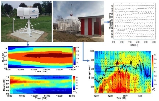
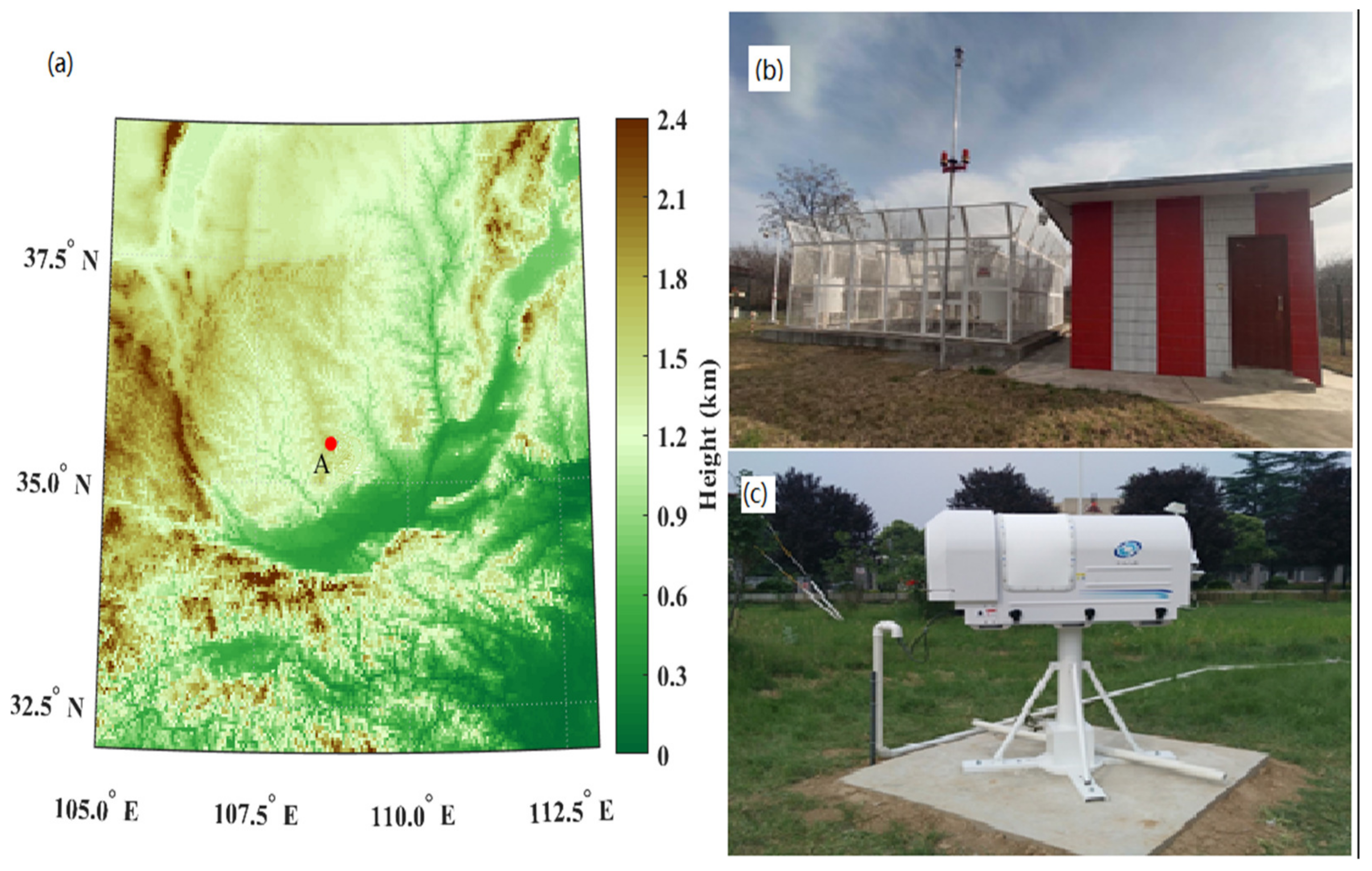
The main instruments used in this study were a wind-profiling radar (CFL), microwave radiometer and an ambient particulate monitor. The CFL-03 wind-profiling radar (shown in Figure 1b) is a boundary layer wind-profiling radar, developed by the 23rd Research Institute of China Aerospace Science and Industry Corporation (the parameters are shown in

Table 1. Parameters of CFL-03 boundary layer wind profiling radar.

Parameter Name	Parameter	Parameter Name	High-Mode	Low-Mode
Radar wavelength	227 mm	Pulse width	0.66 μs	0.33 μs
Beam width	8°	Height resolution	120	60
Beam number	5	FFT points	512	256
Antenna gain	25 dB	Receiver band width	1.5 MHz	3.0 MHz
Feeder loss	2 dB	Min detection altitude	600	60
Peak transmitted power	2.36 KW	Number of coherent accumulations	64	100
Noise coefficient	2 dB

). This radar operates stably and can monitor the $C_n^2$, and horizontal wind speeds and wind directions in real time. The microwave radiometer (shown in Figure 1c) was developed by the China Ordnance 206 Institute; it comprises 21 water vapor channels with a frequency range of 22–30 GHz, 14 temperature channels with a frequency range of 51–59 GHz and 1 infrared channel, which can detect the temperature and relative humidity of the vertical height in real time. The ambient particulate monitor can monitor data such as ${\mathrm{PM}}_{2.5}$ and ${\mathrm{PM}}_{10}$ in the atmosphere per hour.

In this study, the detection site was located at Xianyang Airport (point A in Figure 1a), which is surrounded by mountains, and where haze frequently occurs. According to the China Civil Aviation Ground Observation Rules, haze exists when visibility is <7 km and there is low-level relative humidity of <75%. Based on visibility detected by the visibility meter and relative humidity observed by the weather observation instrument, the trained observers recorded 1230 haze events occurred from 2016 to 2021. The specific number of occurrences per month is shown in

Table 2. The monthly haze events at Xianyang Airport from 2016 to 2021.

Year	Jan	Feb	Mar	Apr	May	June	July	Aug	Sep	Oct	Nov	Dec
2016	27	28	25	23	13	10	16	23	18	14	24	30
2017	29	26	21	13	10	13	8	11	13	13	25	31
2018	26	26	25	12	11	9	11	14	8	16	23	29
2019	31	28	18	16	10	9	4	8	16	18	23	26
2020	26	24	19	20	8	9	13	5	11	10	18	22
2021	23	19	20	12	8	5	5	9	5	12	21	25
Sum	162	151	128	96	60	55	57	70	71	83	134	163

, of which the occurrence frequency in December, January and February is relatively high (all more than 150 times), while the occurrence frequency in May, June and July is less (all below 60 times); the time at which the haze events occurred was concentrated between 06:00 BT and 18:00 BT. Moreover, 60 no-haze events (5 per month) from 2020 to 2021 were also analyzed; visibility was >10 km and the record by trained observers was sunny without any other weather conditions.

This study analyzed the L structure of haze events occurring at Xianyang Airport between 08:00 and 18:00 (BT), in the period 2016 to 2021, using the $C_n^2$, horizontal wind, temperature, RH, ${\mathrm{PM}}_{2.5}$, ${\mathrm{PM}}_{10}$ and AQI, jointly detected by the wind-profiling radar, the microwave radiometer and the ambient particulate monitor.

2.2. The Method of Determining the BLH

The BL is a thin layer where the energy and dynamics of the atmosphere interact with the ground; the convective motion of the atmosphere within the BL is significantly greater than that above the BL [36,37]. Due to the relatively stable operation of the CFL, it can effectively detect the high–resolution $C_n^2$, and horizontal wind speeds and wind directions in real time. As the $C_n^2$ detected by the CFL can be expressed as Equation (1) using the temperature structure constant $C_T^2$, the humidity structure constant $C_e^2$ and the temperature and humidity structure change constant $C_{Te}^2$, the $C_n^2$ can effectively reflect the vertical variation characteristics of atmospheric temperature and humidity. Furthermore, the $C_n^2$ is used to determine the BLH, based on the characteristic that the vertical gradient of temperature and humidity within the BL is greater than that above the BL (e.g., Liu et al. [38], Pichugina et al. [39]).

$$C_n^2=a^2{C}_T^2+b^2{C}_e^2-2ab{C}_{Te}^2$$

(1)

As the horizontal wind speed and direction within the BL are significantly different from those above the BL, many previous studies (e.g., Pichugina et al. [40], Vickers et al. [41]) also used the vertical variation characteristics of the horizontal wind speed and wind direction to effectively inverse the BLH.

Based on the previous studies, this paper used the $C_n^2$, and horizontal wind speed and direction detected by the CFL to determine the BLH. The main steps were as follows:

First, the gradient changes ($\Delta C$) of the atmospheric refractive index structure constants between the adjacent vertical bins were calculated, and then the maximum $\Delta C_{max}$ in the vertical height was found. Subsequent to this, the $\Delta C$ at every bin was normalized by dividing $\Delta C_{max}$ to obtain the normal gradient change ($\Delta {\mathrm{C}}_a$). The equations are expressed as Equation (2), in which $C_{i+1}^2$ and $C_i^2$ are the atmospheric refractive index structure constants of the two adjacent vertical bins, respectively.

$$\{\begin{array}{c}\Delta C=C_{i+1}^2-C_i^2\\ \Delta C_a=\Delta C/\Delta C_{max}\end{array}$$

(2)

Second, according to the method used by Liu et al. [38], the wind directions and wind speeds of the three adjacent vertical bins were used to calculate the variances of wind direction and wind speed (respectively expressed as SD and SS), following which the maximum variances of the wind direction and wind speed in the vertical height (respectively expressed as $S{D}_{max}$ and $S{S}_{max}$) were found. Subsequent to this, the SD (SS) were normalized by dividing $S{D}_{max}$ ($S{S}_{max}$) to obtain the normal variances of wind direction and wind speed (respectively expressed as $S{D}_a$ and $S{S}_a$). The equation is expressed as Equation (3).

$$\{\begin{array}{c}S{D}_a=SD/S{D}_{max}\\ S{S}_a=SS/S{S}_{max}\end{array}$$

(3)

Finally, as the BLHs at Xianyang Airport were less than 3000 m, $\Delta {\mathrm{C}}_a$, $S{D}_a$ and $S{S}_a$ at the same height (less than 3000 m) were used to obtain the judgment value HC. The equation is expressed as Equation (4). Moreover, the HCs of different heights were compared to determine the maximum $H{C}_{max}$. The height corresponding to $H{C}_{max}$ was subsequently determined as the BLH.

$$HC=\Delta {\mathrm{C}}_a\times \mathsf{\alpha } + 0.5(S{D}_a+S{S}_a)\times \left(1-\mathsf{\alpha }\right)$$

(4)

In Equation (4), $\mathsf{\alpha }$ is an adjust parameter. Depending on whether the low-atmospheric layer is well-mixed or not, $\mathsf{\alpha }$ can be expressed as Equation (5), in which T expresses Beijing time and m is the detection times per hour of the CFL (m = 12 in this study). When the low-atmospheric layer is not well-mixed, the $\mathsf{\alpha }$ is less than 1 and the BLH is mainly determined by the wind shear around the BLH, especially in the morning (8:00–9:00 BT). However, the $\mathsf{\alpha }$ is equal to 1 and the BLH is determined by the turbulence of the temperature and RH, when the atmospheric layer is well-mixed (13:00–15:00 BT).

$$\alpha =\{ \begin{array}{c}\frac{\left(T-8\right)·m}{60} 8\le T<13\\ 1 13\le T\le 15\\ \frac{\left(T-15\right)·m}{36} 15\le T\le 18\end{array}$$

(5)

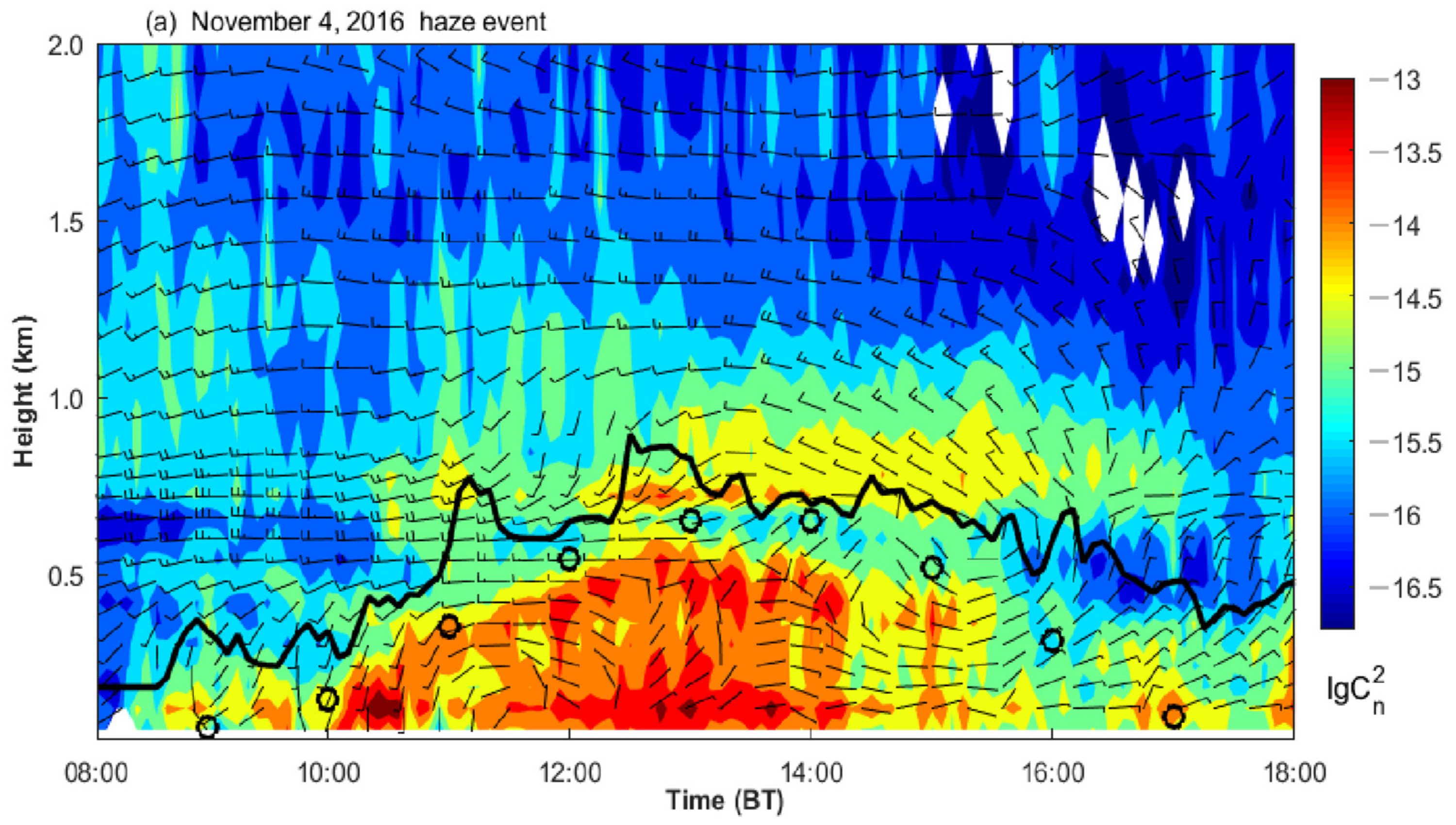
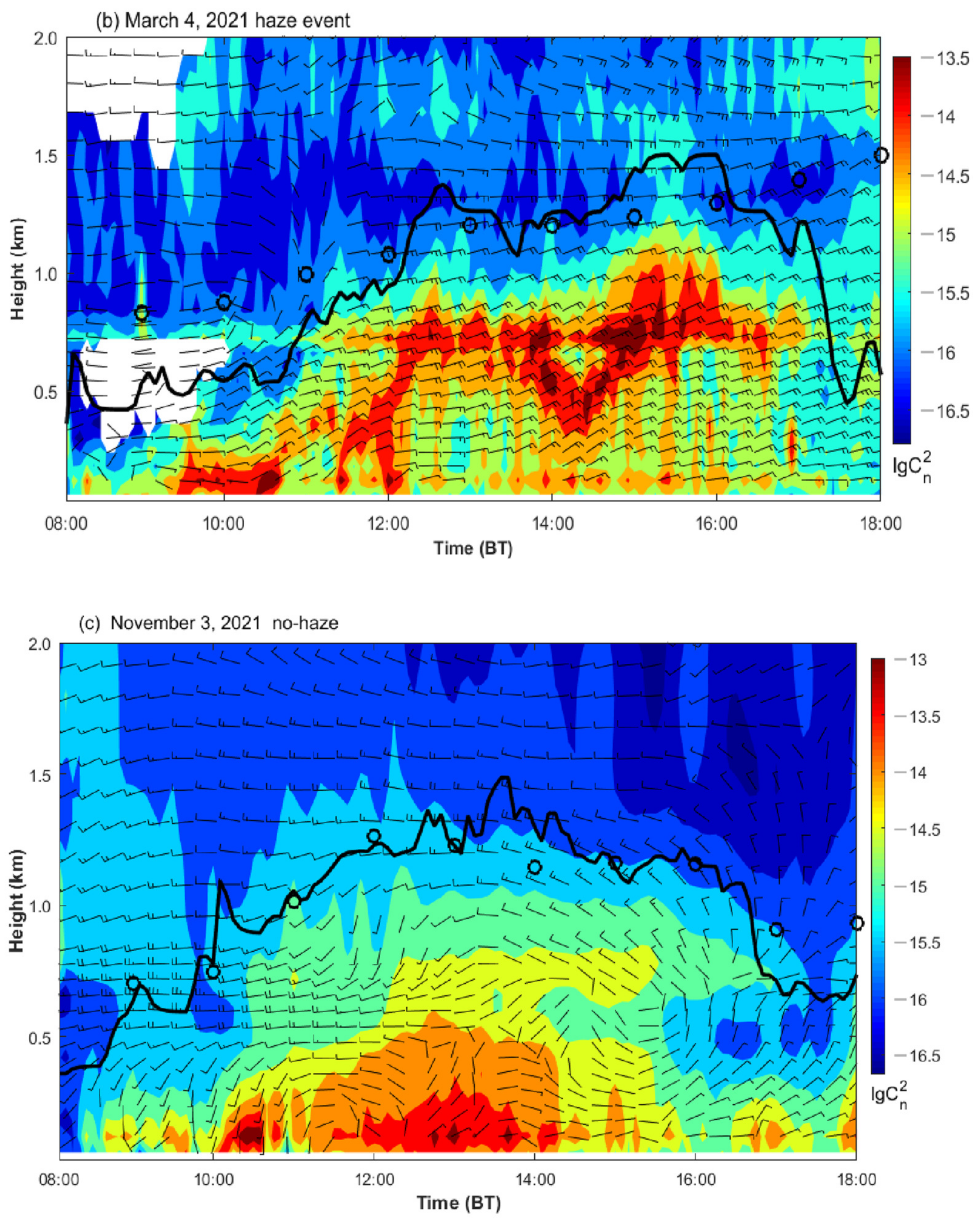
To verify the reliability of this algorithm, two haze events from 8:00 to 18:00 on 4 November 2016 and from 8:00 to 18:00 on 4 March 2021, and one no-haze event from 8:00 to 18:00 on 3 November 2021 were selected to judge the BLHs (black line in Figure 2). Furthermore, compared with the BLHs of the time from 12:00 to 16:00 (black circles in Figure 2 are the reanalysis data from ERA-Interim https://cds.climate.copernicus.eu/cdsapp#!/dataset/reanalysis-era5-single-levels?tab=form), the two data points were consistent, with the difference being less than 100 m, which indicates that the BLH inversion by this algorithm is credible. A more in-depth discussion of this method is found in the Discussion section.

3. Results

3.1. Spatial-Temporal Characteristics of Typical Haze Events within the BL in Different Months

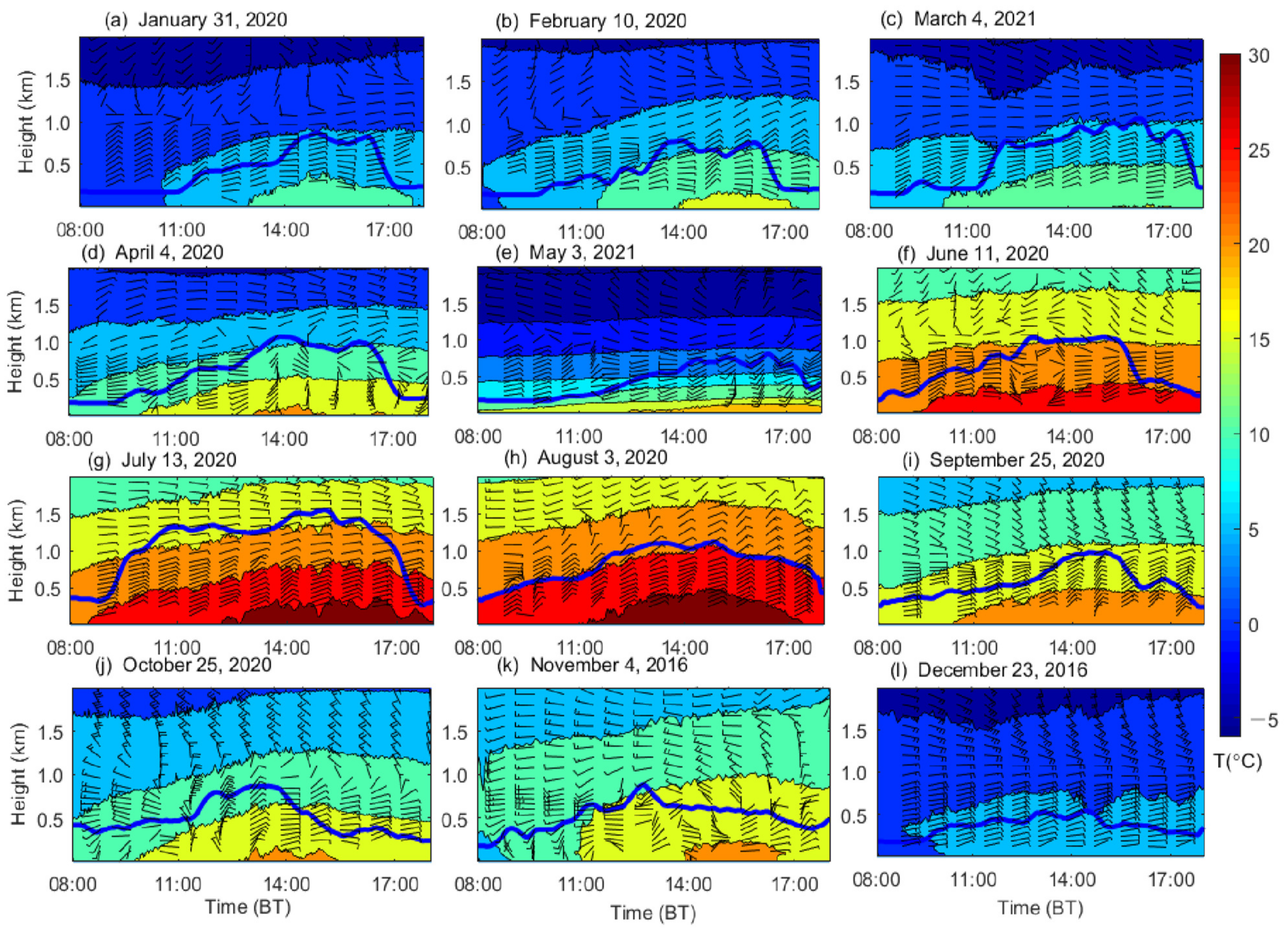
In order to examine the evolution characteristics of the boundary layer structure during the haze events at Xianyang Airport, the haze events occurring on 31 January 2020, 10 February 2020, 4 March 2021, 4 April 2020, 3 May 2021, 11 June 2020, 13 July 2020, 3 August 2020, 25 September 2020, 25 October 2020, 4 November 2016, and 23 December 2016, were selected as typical cases for different months. Their corresponding data were used in the analysis of the spatial–temporal evolution characteristics of temperature, relative humidity, and wind.

3.1.1. Spatial–Temporal Characteristics of Temperature and Horizontal Wind within the BL during Typical Haze Events

The spatial–temporal evolution of the temperature and horizontal wind within the BL in the typical haze process at Xianyang Airport were obtained using temperature and wind data detected by the microwave radiometer or the CFL. As shown in Figure 3 (the blue lines are the BLHs with time), at the start of sunrise (8:00–9:00), the ground temperature was very low, and the low altitude was a stable boundary layer with a low BLH (less than 500 m). Furthermore, with the increase in solar radiation (9:00–12:00), the ground temperature gradually increased, and the BLH also increased gradually. Subsequently, when time reached noon (13:00–15:00), the temperature reached its maximum value, with the BLH also reaching its maximum. However, as the solar radiation began to weaken after noon (16:00–17:00), the temperature began to fall and the BLH gradually decreased. When the sun began to set (18:00), the temperature fell significantly, with the BLH falling to 500 m again.

Comparing July with the highest temperature (Figure 3g) and January with the lowest temperature (Figure 3a), it is seen that the ground heated more rapidly with time than it did in January due to the greater intensity of solar radiation in July. During July, the BLH also rose more rapidly and its maximum value reached 1300 m at 14:00. However, during January, the solar radiation intensity was weaker, with the ground temperature increasing slowly; moreover, the corresponding BLH rose slowly and its maximum value was just over 500 m. One explanation is that the higher July temperatures and stronger solar radiation resulted in the sensible heat flux being larger and the effect of turbulence and mining being stronger. Correspondingly, the BLH increased more rapidly and was higher.

As shown in Figure 3, generally, the wind direction within the BL was northeasterly or northwesterly, and the wind speed was lower than 5 m/s. There was also wind shear (changes in wind direction and speed) at the top of the BL. Moreover, the wind speed did not vary much with time, but the wind direction changed significantly from 12:00 to 15:00, which indicates that there was a certain turbulent motion within the BL during this period. Furthermore, this turbulent motion could have accelerated the exchange of heat and the mining of water vapor in the atmosphere, thereby promoting the elevation of BLH. Additionally, when the BLH increased, the turbulent motion within the BL may also have accelerated the mixing of pollutant particles. This probably led to dilution of the concentration of pollutants and reductions in ${\mathrm{PM}}_{2.5}$ and ${\mathrm{PM}}_{10}$ from 12:00 to 15:00.

Overall, the temperature within the BL was significantly higher than that above the BL during the haze events at Xianyang Airport. Moreover, the change in BLH with time positively correlated with temperature. When the temperature increased with time, the BLH also increased; however, when the temperature decreased with time, the BLH also decreased. In addition, the higher temperature and the stronger the solar radiation, the more rapidly and higher the BLH grows. The wind speed within the BL was relatively small (basically lower than 5 m/s) and its variation with time was small during the haze events, which was conducive to the accumulation of pollutants and easy development of haze. In addition, there was some wind shear at the top of the BL.

3.1.2. Spatial—Temporal Characteristics of Relative Humidity within the BL during Typical Haze Events

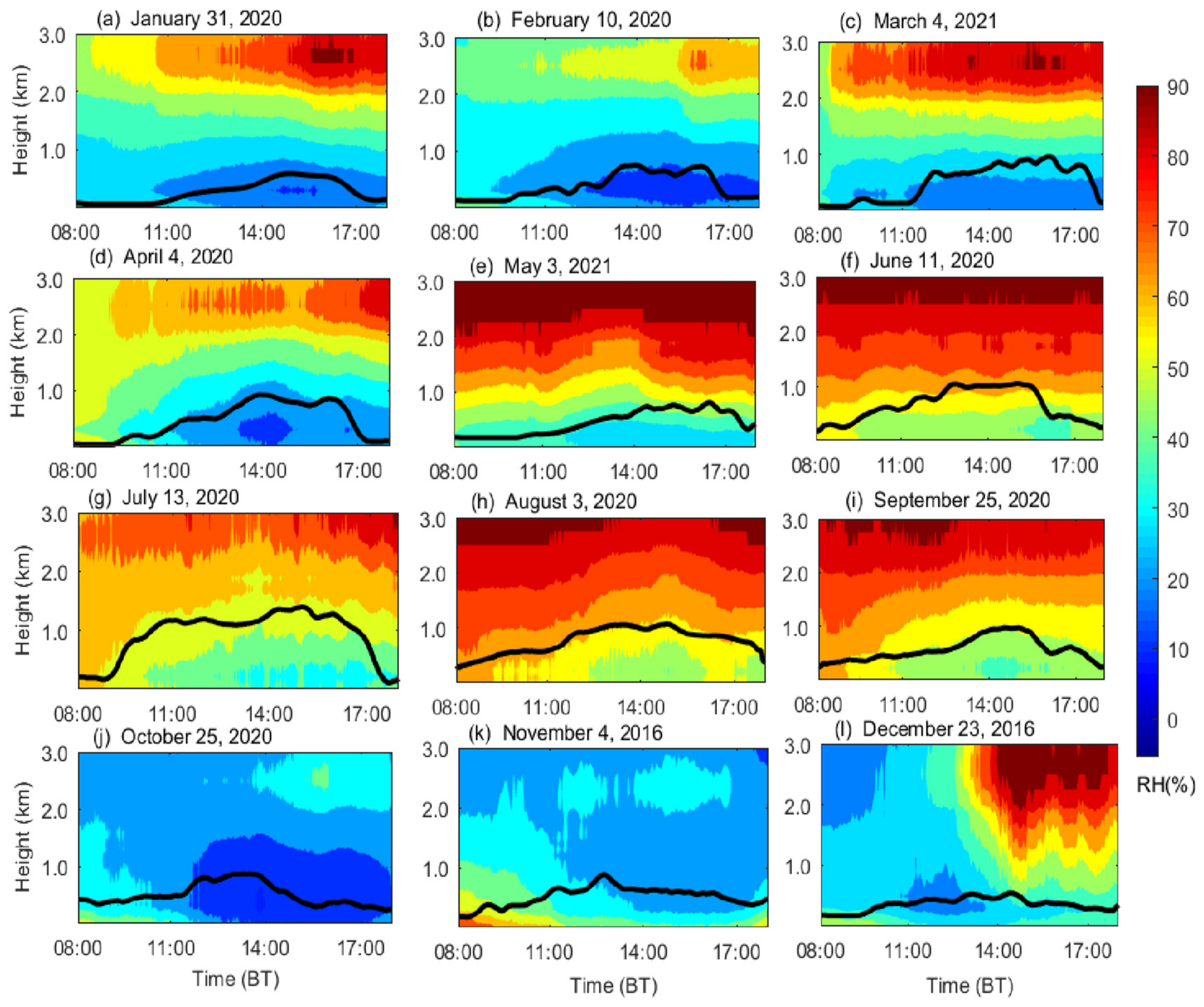
Figure 4 illustrates the spatial–temporal evolution of the relative humidity within the BL of the typical haze process at Xianyang Airport (where the black line is the variety of the BLH with time). Comparing Figure 3 and Figure 4, the characteristics of relative humidity and temperature with time are in opposition. As shown for the period October–December (Figure 4j,k), due to the valley thermal winds from more polluted sites, there were advective processes in the Xianyang airport. Moreover, as the role of the advective processes, the spatial–temporal evolution of relative humidity was not consistent with the BL. In other months, during the hours from 8:00 to 10:00, the relative humidity within the BL was relatively high, while the BLH was relatively low. Moreover, from 10:00 to 14:00, as the BLH gradually increased, the relative humidity within the BL gradually decreased with time. Subsequently, from 16:00 to 18:00, the relative humidity within the BL increased gradually as the BLH decreased with time. One explanation is that, as the water vapor within the BL was fully mixed due to turbulent flow, the space for water vapor to min became larger with the increasing BLH, and the water vapor was diluted; correspondingly, the relative humidity gradually decreased. As seen in Figure 4, the values of relative humidity within the BL were all relatively small. As the height increased, the relative humidity also tended to increase; moreover, the relative humidity within the BL was generally smaller than that above the BL. This may be because when there is low water vapor in the atmosphere (low relative humidity), the vertical variation in specific humidity within the BL is small, so the relative humidity gradually increases with height as the temperature decreases with height (Figure 3).

Overall, the relative humidity within the BL gradually decreased with the increasing BLH during the haze events at Xianyang Airport. However, as the BLH decreased with time, the relative humidity within the BL gradually increased. Moreover, in the vertical direction, the relative humidity within the BL gradually increased with height and was generally lower than that above the BL.

3.2. Statistical Characteristics of Haze

This study used data from 1230 haze and 60 no-haze events, all occurring between 2016 and 2021. These were detected by CFL and microwave radiometer to obtain high-resolution and accurate statistical characteristics of temperature, relative humidity (RH) and wind within the BL of the haze at Xianyang Airport, and then analyzed.

3.2.1. Statistical Characteristics of BLH during Haze Events

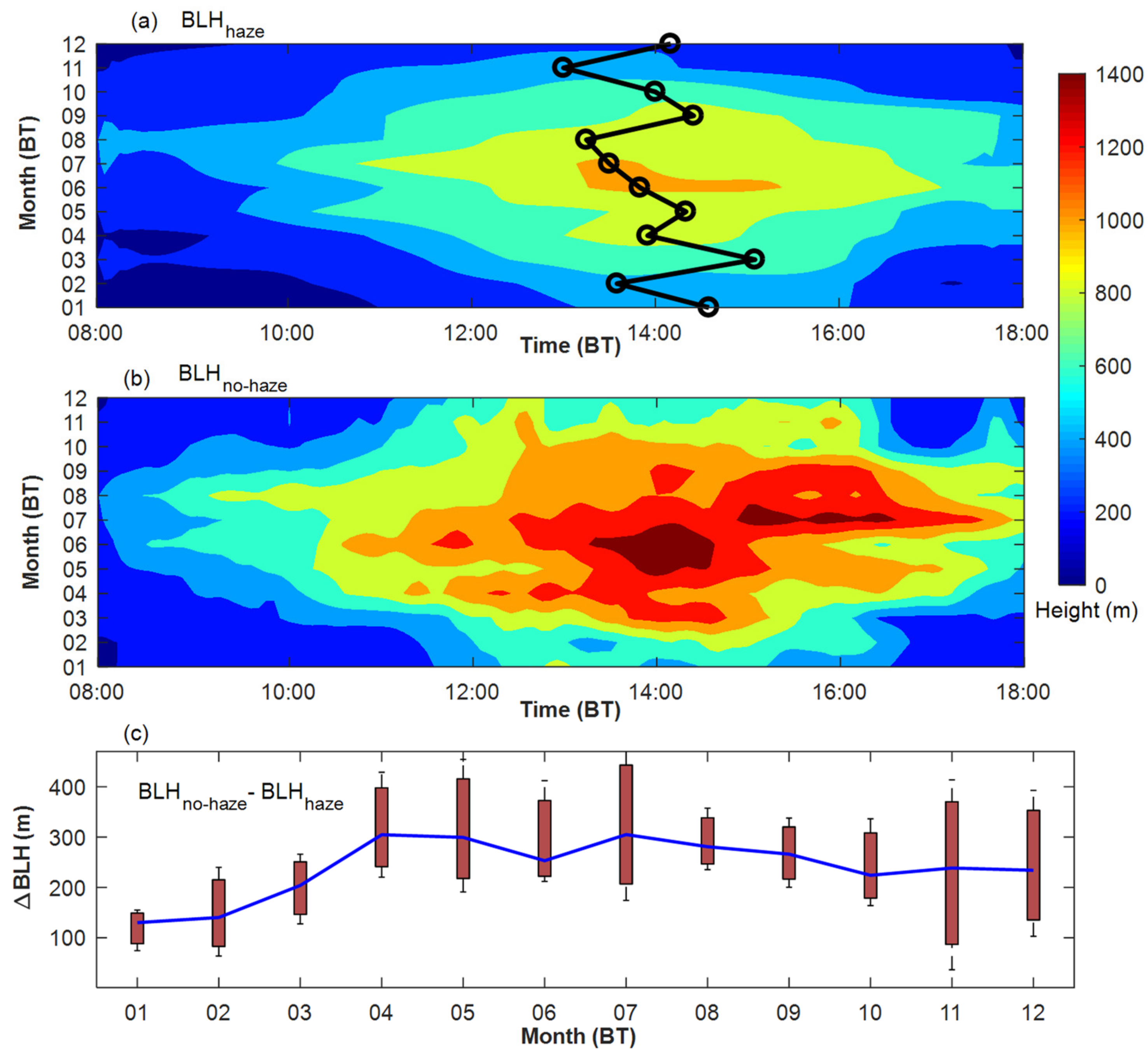
The BLHs of haze events and no-haze events were calculated using the $C_n^2$, the horizontal wind direction and wind speed detected by the CFL. Figure 5 shows the monthly average boundary layer heights of haze events (${\mathrm{BLH}}_{\mathrm{haze}}$) and no-haze events (${\mathrm{BLH}}_{\mathrm{no}-\mathrm{haze}}$), as well as the difference between ${\mathrm{BLH}}_{\mathrm{no}-\mathrm{haze}}$ and ${\mathrm{BLH}}_{\mathrm{haze}}$ (Figure 5c). As shown in Figure 5a, the ${\mathrm{BLH}}_{\mathrm{haze}}$ in June, July and August were higher than in other months at the same time, while the ${\mathrm{BLH}}_{\mathrm{haze}}$ in November, December, January, and February were lower than in other months at the same time. In the morning (8:00–9:00), low altitude with lower solar radiation characterized the stable boundary layer, and the atmospheric structure was very stable; moreover, the ${\mathrm{BLH}}_{\mathrm{haze}}$ was very small in this period, including 200 m in January and December, and 500 m in June and July. After 9:00, the ${\mathrm{BLH}}_{\mathrm{haze}}$ gradually increased with the rising of the sun and the continuous strengthening of solar radiation. For the period 13:00–15:00, the ${\mathrm{BLH}}_{\mathrm{haze}}$ reached the maximum (as shown by the black line in Figure 5a): the maximum ${\mathrm{BLH}}_{\mathrm{haze}}$ in December, January, and February was about 600 m, while the maximum ${\mathrm{BLH}}_{\mathrm{haze}}$ in June and July reached 1100 m, and the maximum ${\mathrm{BLH}}_{\mathrm{a}}$ in other months was between 600 m and 1000 m. After 15:00, the ${\mathrm{BLH}}_{\mathrm{haze}}$ gradually decreased with the continuous weakening of solar radiation. Subsequently, the ${\mathrm{BLH}}_{\mathrm{haze}}$ gradually decreased again to 500 m at 18:00. As shown in Figure 5, the characteristics of ${\mathrm{BLH}}_{\mathrm{haze}}$ and ${\mathrm{BLH}}_{\mathrm{no}-\mathrm{haze}}$ were consistent with time; however, the ${\mathrm{BLH}}_{\mathrm{haze}}$ was lower than ${\mathrm{BLH}}_{\mathrm{no}-\mathrm{haze}}$, with a minimum difference of 150 m in January, and a maximum difference of 300 m in July (as shown in Figure 5c).

In short, the ${\mathrm{BLH}}_{\mathrm{haze}}$ of the haze at Xianyang Airport was generally less than 1000 m, and this was also less than the ${\mathrm{BLH}}_{\mathrm{no}-\mathrm{haze}}$, which indicates that the lower BLH was more favorable for the development of the haze. Moreover, the ${\mathrm{BLH}}_{\mathrm{haze}}$ in December and January was distributed at 200–600 m lower than other months while that in June and July was distributed at 500–1100 m higher than other months and the maximum ${\mathrm{BLH}}_{\mathrm{a}}$ appeared at 13:00–15:00.

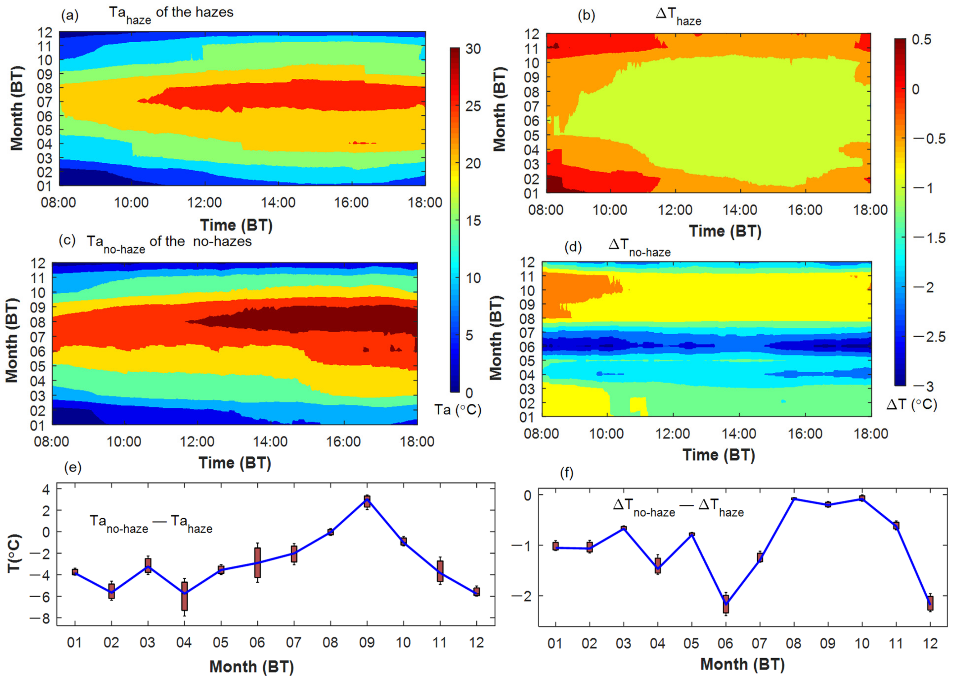
3.2.2. Statistical Characteristics of Temperature within the BL during Haze Events

Figure 6 illustrates the time distribution of the average temperature within the BL of the haze events (${\mathrm{Ta}}_{\mathrm{hzae}}$) and no-haze events (${\mathrm{Ta}}_{\mathrm{no}-\mathrm{hzae}}$). The time distribution of sensible heat flux(the average 100 m vertical temperature difference $\Delta {\mathrm{T}}_{\mathrm{haze}}$ and $\Delta {\mathrm{T}}_{\mathrm{no}-\mathrm{haze}}$) within the BL of haze events and no-haze events were calculated (Figure 6b,d) according to Equation (6), in which ${\mathrm{h}}_1$ and ${\mathrm{h}}_2$ are two adjacent heights (${\mathrm{h}}_1>{\mathrm{h}}_2$), and correspond to the temperatures ${\mathrm{T}}_{{\mathrm{h}}_1}$ and ${\mathrm{T}}_{{\mathrm{h}}_2}$.

$$\{\begin{array}{c}\Delta T=\left({\mathrm{T}}_{{\mathrm{h}}_1}-{\mathrm{T}}_{{\mathrm{h}}_2}\right)/\Delta h\\ \Delta h=\left({\mathrm{h}}_1-{\mathrm{h}}_2\right)/100\end{array}$$

(6)

As shown in Figure 5a and Figure 6a, in the morning (8:00–9:00), the ${\mathrm{Ta}}_{\mathrm{haze}}$ was lower than at other times, with the corresponding ${\mathrm{BLH}}_{\mathrm{haze}}$ also being lower than at other times. After 9:00, as the sun rose and the ${\mathrm{Ta}}_{\mathrm{haze}}$ began to increase, the heat flux gradually increased; meanwhile, the corresponding ${\mathrm{BLH}}_{\mathrm{haze}}$ also gradually increased. Furthermore, during the period 13:00–15:00, the ${\mathrm{Ta}}_{\mathrm{haze}}$ reached its maximum, with the corresponding ${\mathrm{BLH}}_{\mathrm{haze}}$ also reaching its maximum. However, the ${\mathrm{Ta}}_{\mathrm{haze}}$ began to decrease, with the ${\mathrm{BLH}}_{\mathrm{haze}}$ decreasing gradually after 16:00. Until 18:00, the ${\mathrm{Ta}}_{\mathrm{haze}}$ clearly fell and the corresponding ${\mathrm{BLH}}_{\mathrm{haze}}$ fell to 500 m. In addition, for the same time (same abscissa in Figure 6a), the months with a larger ${\mathrm{T}}_{\mathrm{a}}$ (June, July, and August) correspond to the higher ${\mathrm{BLH}}_{\mathrm{haze}}$, while the months with a lower ${\mathrm{T}}_{\mathrm{a}}$ (January, February, and December) correspond to the lower ${\mathrm{BLH}}_{\mathrm{haze}}$. These correlations indicate that the changes in low-level temperature exert a strong influence on the development of the BLH. When the temperature increased, the low-altitude energy interaction intensified, which led to the enhancement of turbulent motion and promoted the development of BLH. However, when the temperature decreased, the low-level energy interaction weakened and the turbulent motion also decreased, which suppressed the development of BLH. Comparing Figure 6a,c, it is seen that the characteristics of ${\mathrm{Ta}}_{\mathrm{haze}}$ and ${\mathrm{Ta}}_{\mathrm{no}-\mathrm{haze}}$ are consistent with time; moreover, ${\mathrm{Ta}}_{\mathrm{haze}}$ was larger than ${\mathrm{Ta}}_{\mathrm{no}-\mathrm{haze}}$ during the months except September, in which the haze events always occurred after precipitation that led to the ${\mathrm{Ta}}_{\mathrm{haze}}$ being lower than the ${\mathrm{Ta}}_{\mathrm{no}-\mathrm{haze}}.$ As shown in Figure 6e, the maximum difference between ${\mathrm{Ta}}_{\mathrm{haze}}$ and ${\mathrm{Ta}}_{\mathrm{no}-\mathrm{haze}}$ was 6 °C in February, and the min difference in ${\mathrm{Ta}}_{\mathrm{haze}}{ \mathrm{and} \mathrm{Ta}}_{\mathrm{no}-\mathrm{haze}}$ was less than 1 ℃ in August.

As shown in Figure 6b, the $\Delta {\mathrm{T}}_{\mathrm{haze}}$ was mainly distributed in the range of −0.9 °C–0.4 °C. In the morning (8:00–9:00), the $\Delta {\mathrm{T}}_{\mathrm{haze}}$ within the BL was greater than 0 °C in January, February, November, and December, with an inversion layer at low altitude; meanwhile, the $\Delta {\mathrm{T}}_{\mathrm{haze}}$ was also very small (less than −0.2 °C) in the other months. This indicates that the low altitude was very stable. Meanwhile, the atmospheric structure was a stable BL during this period. Furthermore, after 9:00, due to the continuous heating of the ground temperature, the temperature inversion layer disappeared and the $\Delta {\mathrm{T}}_{\mathrm{haze}}$ within the BL began to grow; meanwhile, the low altitude changed from a stable BL to a mixed BL. Moreover, between 13:00 and 15:00, the $\Delta {\mathrm{T}}_{\mathrm{haze}}$ within the BL reached a maximum (−0.9 °C in June, July, and August, and about −0.4 °C in January and December) with the heat mining effect reaching the maximum, and the corresponding BLH also reaching its maximum. After 16:00, the $\Delta {\mathrm{T}}_{\mathrm{haze}}$ within the BL gradually decreased with the heat mining effect at low altitude becoming weaker, and the BLH also gradually decreased. Comparing Figure 6b,d,f, it can be observed that $\Delta {\mathrm{T}}_{\mathrm{haze}}$ was lower than $\Delta {\mathrm{T}}_{\mathrm{no}-\mathrm{haze}}$; moreover, the maximum difference in $\Delta {\mathrm{T}}_{\mathrm{haze}} \mathrm{and} \Delta {\mathrm{T}}_{\mathrm{no}-\mathrm{haze}}$ was 2 ℃ in June, and the min difference in $\Delta {\mathrm{T}}_{\mathrm{haze}} \mathrm{and} \Delta {\mathrm{T}}_{\mathrm{no}-\mathrm{haze}}$ was less than 0.2 ℃ in August. These results indicate that the sensible heat flux of the haze was less than that of the no-haze, and the atmospheric structure for the haze was more stable than that for no-haze.

Overall, the ${\mathrm{Ta}}_{\mathrm{haze}}$ was larger than the ${\mathrm{Ta}}_{\mathrm{no}-\mathrm{haze}},$ and the $\Delta {\mathrm{T}}_{\mathrm{haze}}$ at low altitude was smaller than the $\Delta {\mathrm{T}}_{\mathrm{no}-\mathrm{haze}}$. Meanwhile, the atmospheric structure for haze events was more stable than that for no-haze events.

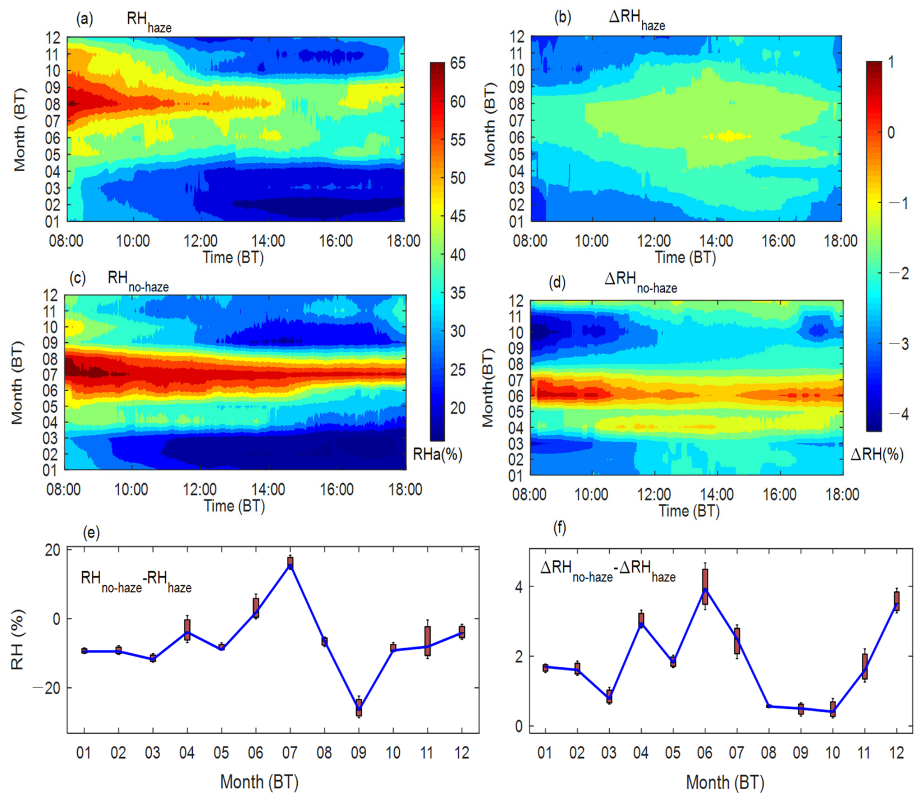
3.2.3. Statistical Characteristics of Relative Humidity within the BL during Haze Events

Figure 7 shows the distributions of the average relative humidity (${\mathrm{RH}}_{\mathrm{haze}}$ and ${\mathrm{RH}}_{\mathrm{no}-\mathrm{haze}}$), and the average 100 m vertical relative humidity difference ($\Delta {\mathrm{RH}}_{\mathrm{haze}}$ and $\Delta {\mathrm{RH}}_{\mathrm{no}-\mathrm{haze}}$) within the BL. As shown in Figure 7a,c, it can be observed that the ${\mathrm{RH}}_{\mathrm{haze}}$ of haze events at Xianyang Airport was generally lower than 65% and higher than ${\mathrm{RH}}_{\mathrm{no}-\mathrm{haze}}$, except in July. As shown in Figure 7e, the maximum difference in ${\mathrm{RH}}_{\mathrm{haze}}$ and ${\mathrm{RH}}_{\mathrm{no}-\mathrm{haze}}$ was 20% in September, and the min difference in ${\mathrm{RH}}_{\mathrm{haze}}$ and ${\mathrm{RH}}_{\mathrm{no}-\mathrm{haze}}$ was less than 5% in June. Moreover, the ${\mathrm{RH}}_{\mathrm{haze}}$ was distributed between 20% and 40% in January and February, while the ${\mathrm{RH}}_{\mathrm{haze}}$ was distributed between 40% and 65% in July, August, and September. During late autumn and winter, Xianyang Airport was under the control of a weak high ridge, with a stable atmospheric structure and little precipitation, so the was low. However, the haze events at Xianyang Airport mostly occurred after precipitation during the autumn, so the ${\mathrm{RH}}_{\mathrm{haze}}$ was higher. In terms of temporal variability, the ${\mathrm{RH}}_{\mathrm{haze}}$ was higher in the morning (8:00–9:00) than at other times, and the corresponding BLH was lower and the air pollution was more serious. After 9:00, the ${\mathrm{RH}}_{\mathrm{haze}}$ decreased gradually with increasing BLH due to the strengthening of the mixing effect and the dilution of water vapor. For the period 13:00–15:00, the ${\mathrm{RH}}_{\mathrm{haze}}$ decreased to a minimum, with the BLH reaching a maximum. After 17:00, there was some increase in the ${\mathrm{RH}}_{\mathrm{haze}}$ within the BL. In short, the larger the relative humidity, the lower the BLH, with more serious air pollution.

As shown in Figure 7b, the $\Delta R{H}_{haze}$ in January, February, November, and December was distributed in the range of −1~1%, and that in March, April, May, and October was distributed in the range of 0~1.5%; the $\Delta R{H}_{haze}$ in June, July and August was distributed in the range of 1.5~3%. As shown in Figure 7f, the $\Delta R{H}_{haze}$ was lower than the $\Delta R{H}_{no-haze}$, which indicates the water vapor interaction in the haze events was less than that in the no-haze events. In the morning (8:00–9:00), the $\Delta R{H}_{haze}$ was smaller than at other times. After 9:00, the $\Delta R{H}_{haze}$ increased gradually as the BLH increased, reaching its maximum at 13:00–15:00; subsequently, the $\Delta R{H}_{haze}$ gradually decreased after 16:00. Comparing Figure 6b and Figure 7b, it is observed that the $\Delta R{H}_{haze}$ varied in the opposite manner to the $\Delta T_{haze}$, in that the $\Delta R{H}_{haze}$ was negative, while the $\Delta T_{haze}$ was positive at 8:00–9:00 in January, February, November, and December. Moreover, $\Delta R{H}_{haze}$ in other months had a small positive value, while the corresponding had a small negative value during this period. It is possible that the specific humidity within the BL varied little with height; furthermore, when the temperature gradually increases (decreases) with height, the corresponding relative humidity will gradually decrease (increase) with height.

3.2.4. Statistical Characteristics of Wind within the BL during Haze Events

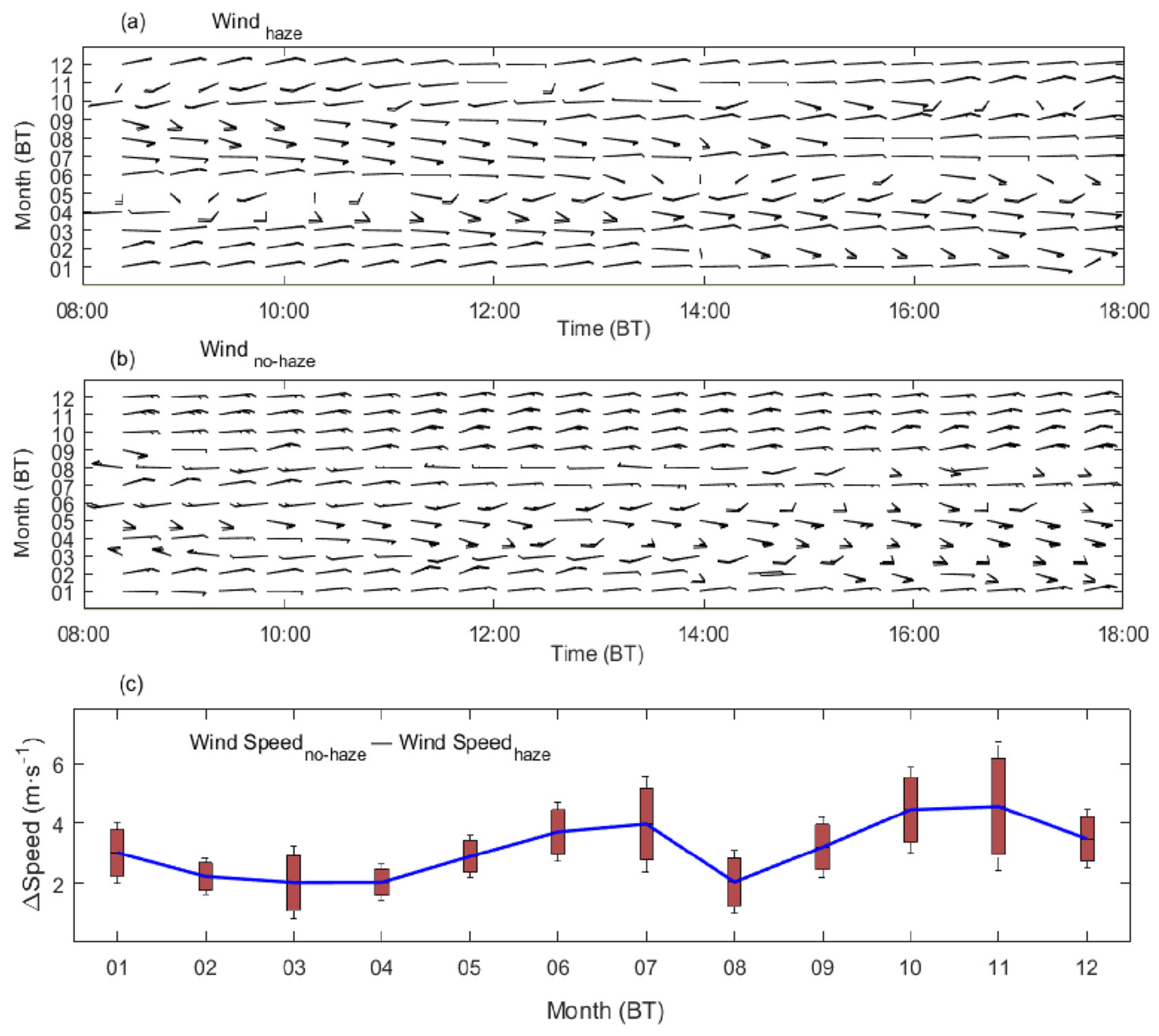
Figure 8 shows the average horizontal wind speed and wind direction within the BL during the haze events and no-haze events in different months. It is observed in Figure 8a that the average wind speed within the BL was less than 4 m/s during haze events and did not vary much with time, which was conducive to the development of haze.

Comparing Figure 8a,b, it can be seen that $wind spee{d}_{haze}$ was lower than $wind spee{d}_{no-haze}$, and $wind directio{n}_{haze}$ was consistent with $wind directio{n}_{no-haze}$. Moreover, the maximum difference between $wind spee{d}_{haze}$ and $wind spee{d}_{no-haze}$ was 4 m/s in November, and the minimum difference was 2 m/s in August (shown in Figure 8c). These results indicate that the low-level turbulence of the haze events was less than that of the no-haze events. Due to the cold air from the north, the dominant wind direction was generally northeaster in December, January, February, and March; moreover. Due to the warm air from the south, the dominant wind direction was generally southeaster or southwester in April, May, June, July, and August. However, in September and October, the dominant wind direction was northeaster or west and the wind speed was very weak due to there was not obvious cold or warm air. Meanwhile, from 8:00 to 11:00, the wind direction changed little with time, indicating that the atmospheric turbulent motion was small and the corresponding BLH was also low. Furthermore, after 16:00, the average horizontal wind direction varied little with time, and the atmospheric structure became relatively stable, with the corresponding BLH about 500 m.

3.3. The Relationship between Haze BLH and the Atmospheric Environment

3.3.1. The Relationship between Haze BLH and AQI

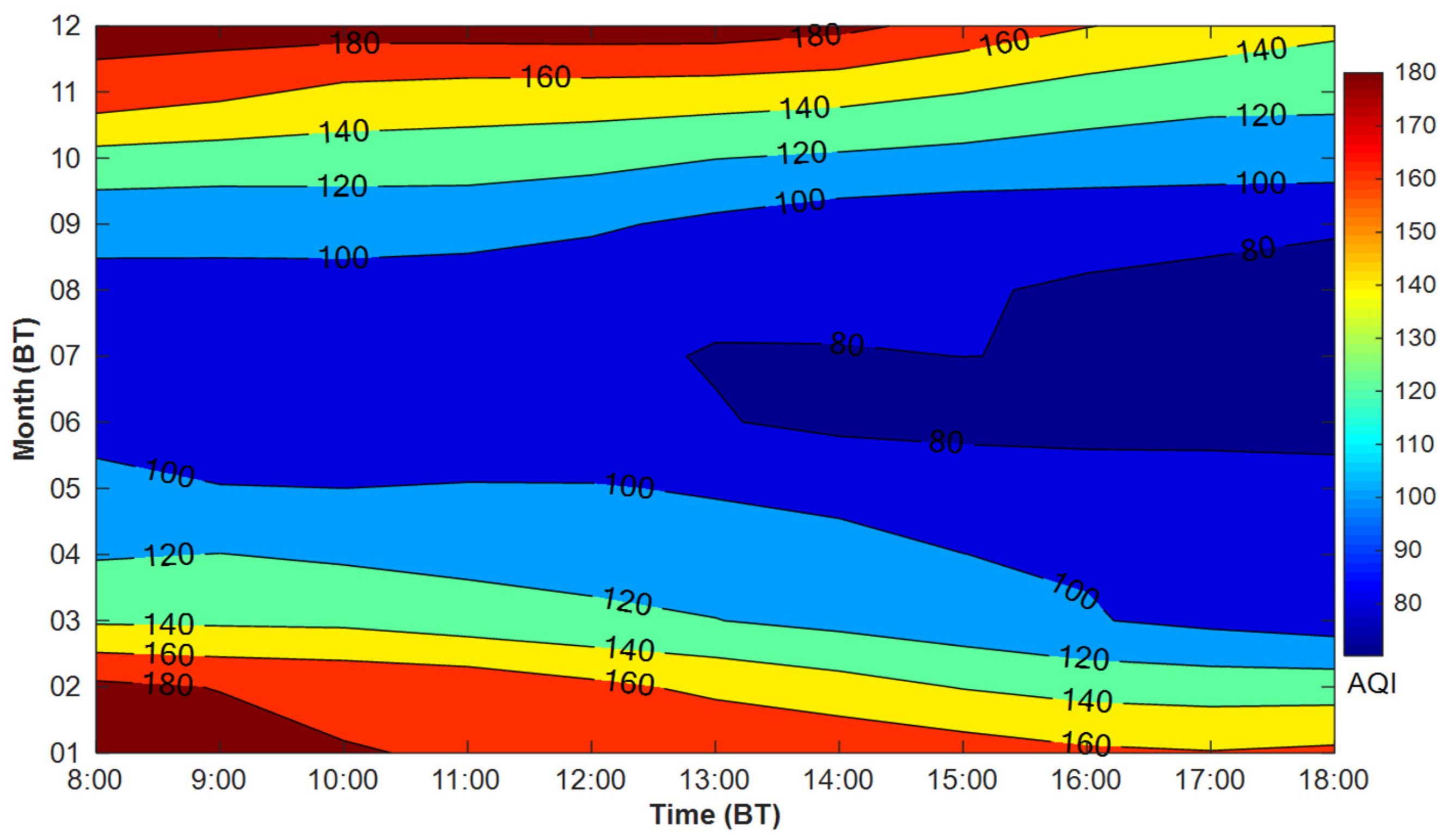
To further analyze the relationship between the haze BLH and air quality, the AQI of 1230 haze events were classified and then averaged by time to obtain Figure 9. Comparing Figure 5 and Figure 9, during December, January, and February—months with a low ${\mathrm{BLH}}_{\mathrm{haze}}$, the average AQI was distributed in the range of 140~190 and the air pollution was severe; however, during June, July, and August—months with a high ${\mathrm{BLH}}_{\mathrm{haze}}$, the average AQI was distributed in the range of 70~100 with lighter air pollution. In short, the months with a lower ${\mathrm{BLH}}_{\mathrm{haze}}$ correspond to larger average AQI.

In the morning (8:00–9:00), due to the stable atmospheric structure with the low BLH, the average AQI was relatively high and the air pollution was severe. Moreover, during the period from 9:00 to 12:00, the average AQI slowly decreased with the continuously increasing BLH. From 12:00 to 15:00, as the BLH reached its maximum, the atmospheric turbulence movement was relatively intense and the average AQI fell rapidly, which was conducive to the dissipation of the haze and better air quality. After 16:00, as the BLH gradually decreased, the average AQI did not change much with time, and the air quality was very good.

Overall, the larger the average AQI, the worse the air quality and the more severe the air pollution; meanwhile, the corresponding BLH was lower and the atmospheric structure was more stable. However, when the BLH became progressively higher with time, the average AQI became progressively smaller, and the air quality progressively improved.

3.3.2. The Relationship between Haze BLH and ${\mathrm{PM}}_{2.5}$ and ${\mathrm{PM}}_{10}$

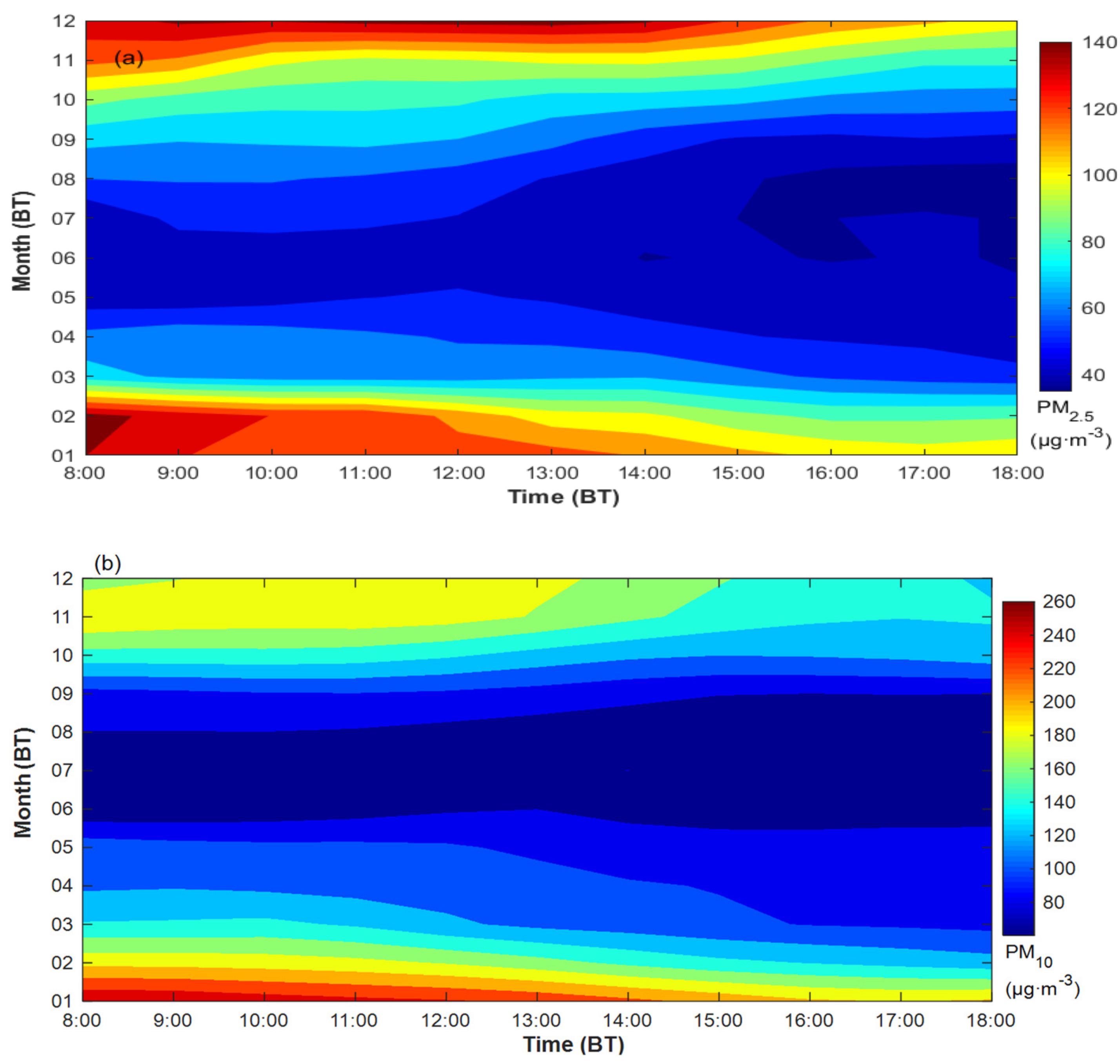
To reveal the relationships between BLH, ${\mathrm{PM}}_{2.5}$ and ${\mathrm{PM}}_{10}$ during the haze events, we obtained the average temporal distributions of ${\mathrm{PM}}_{2.5}$ and ${\mathrm{PM}}_{10}$ (shown in Figure 10). As shown in Figure 10, the trends for the average ${\mathrm{PM}}_{2.5}$ and ${\mathrm{PM}}_{10}$ with time were consistent. In January, with the lowest BLH, the average ${\mathrm{PM}}_{2.5}$ was distributed from 100 $\mathsf{\mu }\mathrm{g}·{\mathrm{m}}^{-3}$ to 140 $\mathsf{\mu }\mathrm{g}·{\mathrm{m}}^{-3}$, and the average ${\mathrm{PM}}_{10}$ was distributed from 180 $\mathsf{\mu }\mathrm{g}·{\mathrm{m}}^{-3}$ to 260 $\mathsf{\mu }\mathrm{g}·{\mathrm{m}}^{-3}$, both being larger than in the other months. However, in July with the highest BLH, the average ${\mathrm{PM}}_{2.5}$ was distributed from 40 μg·m⁻³ to 60 $\mathsf{\mu }\mathrm{g}·{\mathrm{m}}^{-3}$, and the average ${\mathrm{PM}}_{10}$ was distributed from 70 $\mathsf{\mu }\mathrm{g}·{\mathrm{m}}^{-3}$ to 90 $\mathsf{\mu }\mathrm{g}·{\mathrm{m}}^{-3}$, both being lower than in the other months. In short, the average ${\mathrm{PM}}_{2.5}$ and ${\mathrm{PM}}_{10}$ of the month with the higher ${\mathrm{BLH}}_{\mathrm{haze}}$ (Figure 5a) and higher $T{a}_{haze}$ (Figure 6a) were lower than those of the other months at the same time (the same abscissa in Figure 10).

Comparing Figure 5 and Figure 10, the average ${\mathrm{PM}}_{2.5}$ and ${\mathrm{PM}}_{10}$ demonstrate opposite trends to the ${\mathrm{BLH}}_{\mathrm{haze}}$ with time. In the morning (8:00–9:00), the stable atmospheric structure with the low BLH_haze was prone to the accumulation of pollution, which led to the average ${\mathrm{PM}}_{2.5}$ and ${\mathrm{PM}}_{10}$ being larger than those for other periods. After 9:00, the average ${\mathrm{PM}}_{2.5}$ and ${\mathrm{PM}}_{10}$ decreased gradually with the increasing ${\mathrm{BLH}}_{\mathrm{haze}}$. Furthermore, between 13:00 and 15:00, the ${\mathrm{BLH}}_{\mathrm{haze}}$ reached its maximum, thereby producing more space for pollutant mixing and dilution, so the average ${\mathrm{PM}}_{2.5}$ and ${\mathrm{PM}}_{10}$ were reduced. However, there were small changes in the average ${\mathrm{PM}}_{2.5}$ and ${\mathrm{PM}}_{10}$ after 16:00. Overall, the lower the BLH, the more stable the atmospheric structure and the larger the average ${\mathrm{PM}}_{2.5}$ and ${\mathrm{PM}}_{10}$; however, the more serious was the atmospheric pollution.

4. Discussion

The bulk Richardson number-based method (Ri) used in ERA5 is widely used to detect a “well-mixed” BLH [42,43]; however, the Ri is unable to accurate determine the BLH when the atmospheric layer is not well-mixed. Hence, the ERA5 BLH can be used to verify the method used in our study for the period 12:00–16:00 BT.

In this study, we combined the $C_n^2$, and horizontal wind speed and direction to create a method of determining the BLH, considering temperature, RH, and wind. Meanwhile, the adjust parameter ($\mathsf{\alpha }$ in Equations (4) and (5) assumed a different value based on whether the low-level atmospheric layer was well-mixed or not. By comparing against ERA5, our method is basically shown to be credible for the well-mixed BLH. Meanwhile, our method is also credible theoretically, when there is a strong wind shear around the not-well-mixed BLH. Based on previous studies [40,41], there are wind shears around the BLH in the most cases. Overall, the BLHs retrieved by our method are basically credible.

5. Conclusions

In this study, the combined data detected by using a wind-profiling radar, microwave radiometer and atmospheric particulate monitor during 1230 haze events and 60 no-haze events, occurring at Xianyang Airport, were analyzed. The main conclusions are as follows:

(1)

The ${\mathrm{BLH}}_{\mathrm{haze}}$ was generally lower than 1000 m and the ${\mathrm{BLH}}_{\mathrm{no}-\mathrm{haze}}$; moreover, the lower ${\mathrm{BLH}}_{\mathrm{haze}}$ in December and January was distributed in the range of 200–600 m, while the higher ${\mathrm{BLH}}_{\mathrm{haze}}$ in June and July was distributed in the range of 500–1100 m; meanwhile, the max ${\mathrm{BLH}}_{\mathrm{haze}}$ appeared at 13:00–15:00.

(2)

When the ${\mathrm{Ta}}_{\mathrm{haze}}$ was higher, the heat interaction was stronger, the turbulent motion of the atmosphere was more intense and the corresponding BLH was higher. Conversely, when the ${\mathrm{Ta}}_{\mathrm{haze}}$ was lower, the heat interaction between ground and air quality was weaker; moreover, the atmospheric structure was more stable and the corresponding BLH was lower.

(3)

When the BLH rose, the ${\mathrm{RH}}_{\mathrm{haze}}$ gradually decreased, and the ${\mathrm{RH}}_{\mathrm{haze}}$ gradually increased with height; conversely, when the BLH decreased, the ${\mathrm{RH}}_{\mathrm{haze}}$ gradually increased; moreover, the larger the RH, the lower the BLH, and the more serious the air pollution.

(4)

Due to the relatively stable atmospheric structure with the low BLH, the average AQI, ${\mathrm{PM}}_{2.5}$ and ${\mathrm{PM}}_{10}$, were large, the air quality was poor, and the air pollution was severe. However, when the BLH gradually became higher with time, the average AQI, ${\mathrm{PM}}_{2.5}$ and ${\mathrm{PM}}_{10},$ gradually decreased and the air quality gradually improved.

References

- Hua, W.; Wu, B. Atmospheric circulation anomaly over mid– and high– latitudes and its association with severe persistent haze events in Beijing. Atmos. Res. 2022, 277, 106315. [Google Scholar] [CrossRef]
- Qiu, Y.; Gai, P.X.; Yue, F.; Zhang, Y.Y.; He, P.Z.; Kang, H.; Yu, X.W.; Chen, J.B.; Xie, Z.Q. Potential factors impacting PM2.5-Hg during haze evolution revealed by mercury isotope: Emission sources and photochemical processes. Atmos. Res. 2022, 277, 106318. [Google Scholar] [CrossRef]
- Zhang, R.H.; Qiang, L.I.; Zhang, R.N. Meteorological conditions for the persistent severe fog and haze event over eastern China in January 2013. Sci. China Earth Sci. 2014, 57, 26–35. [Google Scholar] [CrossRef]
- Lin, Z.; Wang, Y.H.; Zheng, F.X.; Zhou, Y.; Guo, Y.; Feng, Z.; Li, C.; Zhang, Y.; Hakala, S.; Chan, T.; et al. Rapid mass growth and enhanced light extinction of atmospheric aerosols during the heating season haze episodes in Beijing revealed by aerosol–chemistry–radiation–boundary layer interaction. Atmos. Chem. Phys. 2021, 21, 12173–12187. [Google Scholar] [CrossRef]
- Wang, Y.; Gao, W.; Wang, S.; Song, T.; Gong, Z.; Ji, D.; Wang, L.; Liu, Z.; Tang, G.; Huo, Y.; et al. Contrasting trends of PM2:5 and surface ozone concentrations in China from 2013 to 2017. Natl. Sci. Rev. 2020, 7, 1331–1339. [Google Scholar] [CrossRef] [Green Version]
- An, Z.; Huang, R.-J.; Zhang, R.; Tie, X.; Li, G.; Cao, J.; Zhou, W.; Shi, Z.; Han, Y.; Gu, Z.; et al. Severe haze in northern China: A synergy of anthropogenic emissions and atmospheric processes. Proc. Natl. Acad. Sci. USA 2019, 116, 8657–8666. [Google Scholar] [CrossRef] [Green Version]
- Yang, Y.; Liu, X.; Qu, Y.; Wang, J.; An, J.; Zhang, Y.; Zhang, F. Formation mechanism of continuous extreme haze episodes in the megacity Beijing, China, in January 2013. Atmos. Res. 2015, 155, 192–203. [Google Scholar] [CrossRef]
- Ma, Y.; Ye, J.; Xin, J.; Zhang, W.; de Arellano, J.V.-G.; Wang, S.; Zhao, D.; Dai, L.; Ma, Y.X.; Wu, X.; et al. The Stove, Dome, and Umbrella Effects of Atmospheric Aerosol on the Development of the Planetary Boundary Layer in Hazy Regions. Geophys. Res. Lett. 2020, 47, e2020GL087373. [Google Scholar] [CrossRef]
- Li, M.; Wang, T.; Xie, M.; Zhuang, B.; Li, S.; Han, Y.; Chen, P. Impacts of aerosol-radiation feedback on local air quality during a severe haze episode in Nanjing megacity, eastern China. Tellus B 2017, 69, 1339548. [Google Scholar] [CrossRef] [Green Version]
- Lelieveld, J.; Evans, J.S.; Fnais, M.; Giannadaki, D.; Pozzer, A. The contribution of outdoor air pollution sources to premature mortality on a global scale. Nature 2015, 525, 367–371. [Google Scholar] [CrossRef]
- Spracklen, D.V.; Carslaw, K.S.; Kulmala, M.; Kerminen, V.M.; Sihto, S.L.; Riipinen, I.; Merikanto, J.; Mann, G.W.; Chipperfield, M.P.; Wiedensohler, A.; et al. Contribution of particle formation to global cloud condensation nuclei concentrations. Geophys. Res. Lett. 2008, 35, L06808. [Google Scholar] [CrossRef] [Green Version]
- Chen, H.; Rey, J.; Kwong, C.; Copes, R.; Tu, K.; Villeneuve, P.J.; van Donkelaar, A.; Hystad, P.; Martin, R.V.; Murray, B.J.; et al. Living near major roads and the incidence of dementia, Parkinson’s disease, and multiple sclerosis: A population-based cohort study. Lancet 2017, 389, 718–726. [Google Scholar] [CrossRef]
- Chan, C.K.; Yao, X. Air pollution in megacities in China. Atmos. Environ. 2008, 42, 1–42. [Google Scholar] [CrossRef]
- Slater, J.; Coe, H.; McFiggans, G.; Tonttila, J.; Romakkaniemi, S. The effect of BC on aerosol–boundary layer feedback: Potential implications for urban pollution episodes. Atmos. Chem. Phys. 2022, 22, 2937–2953. [Google Scholar] [CrossRef]
- Liu, C.; Hua, C.; Zhang, H.; Zhang, B.; Wang, G.; Zhu, W.; Xu, R. A severe fog-haze episode in Beijing-Tianjin-Hebei region: Characteristics, sources and impacts of boundary layer structure. Atmos. Pollut. Res. 2019, 10, 1190–1202. [Google Scholar] [CrossRef]
- Kerr, G.H.; Waugh, D.W. Connections between summer air pollution and stagnation. Environ. Res. Lett. 2018, 13, 084001. [Google Scholar] [CrossRef]
- Liu, Q.; Jia, X.; Quan, J.; Li, J.; Li, X.; Wu, Y.; Chen, D.; Wang, Z.; Liu, Y. New positive feedback mechanism between boundary layer meteorology and secondary aerosol formation during severe haze events. Sci. Rep.-UK 2018, 8, 6095. [Google Scholar] [CrossRef] [Green Version]
- Ye, X.; Song, Y.; Cai, X.; Zhang, H. Study on the synoptic flow patterns and boundary layer process of the severe haze events over the North China Plain in January 2013. Atmos. Environ. 2016, 124, 129–145. [Google Scholar] [CrossRef]
- Singh, N.; Solanki, R.; Ojha, N.; Janssen, R.H.H.; Pozzer, A.; Dhaka, S.K. Boundary layer evolution over the central Himalayas from radio wind profiler and model simulations. Atmos. Chem. Phys. 2016, 16, 10559–10572. [Google Scholar] [CrossRef] [Green Version]
- Liu, Y.; Zhang, Y.; Lian, C.; Yan, C.; Feng, Z.; Zheng, F.; Fan, X.; Chen, Y.; Wang, W.; Chu, B.; et al. The promotion effect of nitrous acid on aerosol formation in wintertime in Beijing: The possible contribution of traffic-related emissions. Atmos. Chem. Phys. 2020, 20, 13023–13040. [Google Scholar] [CrossRef]
- Li, J.; Sun, J.; Zhou, M.; Cheng, Z.; Li, Q.; Cao, X.; Zhang, J. Observational analyses of dramatic developments of a severe air pollution event in the Beijing area. Atmos. Chem. Phys. 2018, 18, 3919–3935. [Google Scholar] [CrossRef] [Green Version]
- Wang, Y.; Yao, L.; Wang, L.; Liu, Z.; Ji, D.; Tang, G.; Zhang, J.; Sun, Y.; Hu, B.; Xin, J. Mechanism for the formation of the January 2013 heavy haze pollution episode over central and eastern China. Sci. China Earth Sci. 2014, 57, 14–25. [Google Scholar] [CrossRef]
- Liao, X.; Zhang, X.; Wang, Y. Comparative analysis on meteorological condition for persistent haze cases in summer and winter in Beijing. Environ. Sci. 2014, 35, 2031–2044. (In Chinese). Available online: https://www.hjkx.ac.cn/hjkx/ch/reader/view_abstract.aspx?file_no=20140601&flag=1 (accessed on 20 January 2022).
- Zhao, X.J.; Zhao, P.S.; Xu, J.; Meng, W.; Pu, W.W.; Dong, F.; He, D.; Shi, Q.F. Analysis of a winter regional haze event and its formation mechanism in the North China Plain. Atmos. Chem. Phys. 2013, 13, 5685–5696. [Google Scholar] [CrossRef] [Green Version]
- Wu, Z.; Wang, Y.; Tan, T.; Zhu, Y.; Li, M.; Shang, D.; Wang, H.; Lu, K.; Guo, S.; Zeng, L.; et al. Aerosol Liquid Water Driven by Anthropogenic Inorganic Salts: Implying Its Key Role in Haze Formation over the North China Plain. Environ. Sci. Technol. Lett. 2018, 5, 160–166. [Google Scholar] [CrossRef]
- Cheng, Y.; Zheng, G.; Wei, C.; Mu, Q.; Zheng, B.; Wang, Z.; Gao, M.; Zhang, Q.; He, K.; Carmichael, G.; et al. Reactive nitrogen chemistry in aerosol water as a source of sulfate during haze events in China. Sci. Adv. 2016, 2, e1601530. Available online: https://www.science.org/doi/10.1126/sciadv.1601530 (accessed on 20 January 2022). [CrossRef] [Green Version]
- Tang, G.; Zhang, J.; Zhu, X.; Song, T.; Münkel, C.; Hu, B.; Schäfer, K.; Liu, Z.; Zhang, J.; Wang, L.; et al. Mining layer height and its implications for air pollution over Beijing, China. Atmos. Chem. Phys. 2016, 16, 2459–2475. [Google Scholar] [CrossRef] [Green Version]
- Ding, A.J.; Huang, X.; Nie, W.; Sun, J.N.; Kerminen, V.M.; Petäjä, T.; Su, H.; Cheng, Y.F.; Yang, X.Q.; Wang, M.H.; et al. Enhanced haze pollution by black carbon in megacities in China. Geophys. Res. Lett. 2016, 43, 2873–2879. [Google Scholar] [CrossRef]
- Sun, Y.; Wang, Z.; Fu, P.; Jiang, Q.; Yang, T.; Li, J.; Ge, X. The impact of relative humidity on aerosol composition and evolution processes during wintertime in Beijing, China. Atmos. Environ. 2013, 77, 927–934. [Google Scholar] [CrossRef]
- Kneifel, S.; Redl, S.; Orlandi, E.; Lohnert, U.; Cadeddu, M.P.; Turner, D.D.; Chen, M.-T. Absorption properties of supercooled liquid water between 31 and 225GHz: Evaluation of absorption models using ground-based observations. J. Appl. Meteorol. Climatol. 2014, 53, 1028–1045. [Google Scholar] [CrossRef]
- Kulie, M.S.; Bennartz, R. Utilizing space-borne radars to retrieve dry snowfall. J. Appl. Meteorol. Climatol. 2009, 48, 2564–2580. [Google Scholar] [CrossRef]
- Hocke, K.; Kampfer, N.; Ruffieux, D.; Froidevaux, L.; Parrish, A.; Boyd, I.; von Clarmann, T.; Steck, T.; Timofeyev, Y.M.; Polyakov, A.V.; et al. Comparison and synergy of stratospheric ozone measurements by satellite limb sounders and the ground-based microwave radiometer SOMORA. Atmos. Chem. Phys. 2007, 7, 4117–4131. Available online: https://acp.copernicus.org/articles/7/4117/2007/ (accessed on 20 January 2022). [CrossRef] [Green Version]
- Muller, S.C.; Kampfer, N.; Feist, D.G.; Haefele, A.; Milz, M.; Sitnikov, N.; Schiller, C.; Kiemle, C.; Urban, J. Validation of stratospheric water vapour measurements from the airborne microwave radiometer AMSOS. Atmos. Chem. Phys. 2008, 8, 3169–3183. [Google Scholar] [CrossRef] [Green Version]
- John, V.O.; Buehler, S.A. Comparison of microwave satellite humidity data and radiosonde profiles: A survey of European stations. Atmos. Chem. Phys. 2005, 5, 1843–1853. [Google Scholar] [CrossRef] [Green Version]
- Ming, H.; Wei, M.; Wang, M.; Gao, L.; Chen, L.; Wang, X. Analysis of fog at Xianyang Airport based on multi-source ground-based detection data. Atmos. Res. 2019, 220, 34–45. [Google Scholar] [CrossRef]
- Molod, A.; Salmun, H.; Dempsey, M. Estimating planetary boundary layer heights from NOAA profiler network wind profiler data. J. Atmos. Ocean. Technol. 2015, 32, 1545–1561. [Google Scholar] [CrossRef]
- Garratt, J.R. The atmospheric boundary layer. Earth-Sci. Rev. 1994, 37, 89–134. [Google Scholar] [CrossRef]
- Liu, B.; Guo, J.; Gong, W.; Shi, Y.; Jin, S. Boundary Layer Height as Estimated from Radar Wind Profilers in Four Cities in China: Relative Contributions from Aerosols and Surface Features. Remote Sens. 2020, 12, 1657. [Google Scholar] [CrossRef]
- Pichugina, Y.L.; Banta, R.M. Stable boundary layer depth from high-resolution measurements of the mean wind profile. J. Appl. Meteorol. Climatol. 2010, 49, 20–35. [Google Scholar] [CrossRef]
- Pichugina, Y.L.; Tucker, S.C.; Banta, R.M.; Brewer, W.A.; Kelley, N.D.; Jonkman, B.J.; Newsom, R.K. Horizontal-velocity and variance measurements in the stable boundary layer using Doppler lidar: Sensitivity to averaging procedures. J. Atmos. Ocean. Technol. 2008, 25, 1307–1327. [Google Scholar] [CrossRef]
- Vickers, D.; Mahrt, L. Evaluating formulations of stable boundary layer height. J. Appl. Meteorol. 2004, 43, 1736–1749. [Google Scholar] [CrossRef]
- Zhang, Y.; Gao, Z.; Li, D.; Li, Y.; Zhang, N.; Zhao, X.; Chen, J. On the computation of planetary boundary-layer height using the bulk Richardson number method. Geosci. Model Dev. 2014, 7, 2599–2611. [Google Scholar] [CrossRef] [Green Version]
- Zhou, L.; Tian, Y.; Nei, N.; Ho, S.-P.; Li, J. Rising Planetary Boundary Layer Height over the Sahara Desert and Arabian Peninsula in a Warming Climate. J. Clim. 2021, 34, 4043–4068. [Google Scholar] [CrossRef]
Figure 1.
(a) Location map of Xianyang International Airport; (b) the CFL-03 wind profiling radar; (c) the microwave radiometer.
Figure 2.
Comparison of BLHs (black line) inversed by CFL and BLHs (black circle) from ERA-Interim; (a) 8:00–18:00 on 4 November 2016; (b) 8:00–18:00 on 4 March 2021; (c) no-haze event 8:00–18:00 on 3 November 2021.
Figure 3.
Spatial–temporal evolutions of temperature and horizontal wind during typical haze events; the blue lines are the BLHs with time.
Figure 4.
Spatial–temporal evolutions of relative humidity during typical haze events; the black line is the variation in BLH with time.
Figure 5.
(a) Temporal distribution of the in different months; the black line indicates the time of the highest boundary layer. (b) The temporal distribution of the in different months. (c) Differences in the and .
Figure 6.
Temporal distribution of average temperature within the BL during (a) the haze events , (c) the no-haze events ; the distribution of monthly average sensible heat fluxwithin the BL during (b) the haze events ; (d) the no-haze events in different months; (e) the difference of the and ; (f) the difference of the and .
Figure 7.
Temporal distribution of average relative humidity within the BL during (a) the haze events and (c) the no-haze events ; the distribution of monthly average vertical relative humidity difference within the BL during (b) the haze events and (d) the no-haze events in different months; (e) the difference in the and ; (f) the difference in the and .
Figure 8.
Temporal distribution of average horizontal wind within the BL per half hour during (a) the haze events and (b) the no-haze events in different months; (c) the difference in the and .
Figure 9.
The temporal distribution of the average AQI during haze events in different months.
Figure 10.
(a) The temporal distribution of average during haze events in different months; (b) The temporal distribution of average during haze events in different months.