Direct Target Joint Detection and Tracking Based on Passive Multi-Static Radar

Abstract

Traditional target tracking is carried out based on the point measurements extracted from the radar resolution cells. This is not suitable for situations of low signal-to-noise ratio (SNR). In this paper, we aim to investigate the problem of the joint detection and tracking (JDT) of a target by directly using the received signals of passive multi-static radar without feeding the signals to matched filters. To this end, a novel likelihood function is proposed exploiting the statistical properties of coherent processing between the reference and surveillance signals. With such a likelihood function, the particle Bernoulli filter is employed to perform direct JDT (DJDT) of the target. A remarkable feature of the proposed method is that it is able to achieve satisfactory performance when the SNR of received signals is low. Furthermore, the proposed method cannot only achieve the existence and kinematic state of the target, but also the time-varying SNR of each receiver, which serves as an important input for sensor adjustment. The performance of the proposed method is verified via simulations.

1. Introduction

The passive multi-static radar (PMR) [1], which consists of multiple geographically separated receivers and a non-cooperative transmitter of opportunity, such as a frequency modulation radio [2], television [3], and cell phone base stations [4], to name a few, has the remarkable ability of not emitting additional signals as well as detecting stealth and low-flying targets [5].

Traditional PMR-based area surveillance is divided into two phases: i.e., parameter extraction [6] and target tracking [7,8]. In the former phase the received signals from the surveillance and reference channels are fed to the matched filters, then the measurement resolution cells with a large power/amplitude are announced as the potential targets, resulting in a set of extracted point measurements [9,10]. Then in the latter phase, the time-consecutive measurements are adopted to further detect and form target trajectories [11,12,13]. Such a processing technique works well when the signal-to-noise ratio (SNR) at each receiver is high enough; however, when the SNR is low or the receivers are under interference, target detection and tracking with PMR suffering from performance degradation or even failure [14].

A solution to improve the target tracking performance under low SNR is to make full use of the received signals of reference and surveillance channels, i.e., perform direct target tracking based on the received signals other than conducting a two-step treatment. Such an idea was first known as direct localization in the field of target localization. In [15], a maximum likelihood-based direct localization method was proposed, where the Doppler shift effect was considered to form the likelihood. However, the signal model was not accurate when the signal became the wideband. In [16], the idea of direct localization was applied for through wideband random signals using both the Doppler effect and the time delay, and the corresponding Cramér–Rao bound (CRB) was derived.

In addition to direct target localization, the idea of direct tracking has been developed. Knowing the complex envelope of transmitted waveforms, Ref. [17] provided an extended Kalman filter in a multiple input, multiple output radar system. In [18], a particle filter is presented to directly track a single target illuminated by a digital-video broadcasting terrestrial signal in a PMR system. This algorithm utilizes a single-stage scheme but assumes that the transmitted signal can be estimated perfectly using the reference signal, which is received directly from the transmitter. In [19], a new likelihood was derived on the basis of an unknown deterministic signal and an unknown random Gaussian signal, which is radiated by moving the transmitter impinging on receivers and the posterior CRB (PCRB). In [20], an adaptive Gaussian particle filter was proposed for direct target tracking based on distributed sensor networks, and its further extended work can be referred to in [21], wherein the diffusion strategy has been incorporated for information delivery among sensor networks. In addition, the particle number adaptation strategy has also been discussed. In our previous work [22], direct tracking was accomplished based on a maneuvering single-sensor array exploiting the unscented Kalman filter.

Nevertheless, the aforementioned contributions considered only the problem of direct target tracking, which is based on the assumption that the correct identification of the target may not be a trivial task in low-SNR cases. As has been pointed out in [9,23,24], the incorporation of signal phase information can help to promote the target detection performance, which motives the work of this paper, i.e., developing an algorithm for the direct joint detection and tracking (DJDT) of a target.

To this end, a new likelihood function, which describes the relations between the target state and the cross ambiguity function (CAF) of signals in the reference/surveillance channels [24], is derived. Such a likelihood turns out to be Wishart and it contains the unknown channel coefficients of the receivers. In this paper, the unknown channel coefficients are included into the target state, so that the unknown channel coefficients are estimated jointly with the kinematic state of the target. In order to perform DJDT, the Bernoulli filter [25] is employed with the particle implementation. A remarkable feature of the proposed method is that it can accomplish the DJDT of a target when the signal-to-noise ratio (SNR) becomes extremely low, under which condition the performance of traditional detection and tracking approaches degrades heavily. The effectiveness of the proposed method is verified via simulations.

In summary, the main contributions of this paper are listed as follows:

• A novel likelihood function for the DJDT of a target is proposed.
• The particle Bernoulli filter-based target DJDT approach is proposed.
• An algorithm for the joint estimation of the target kinematic states and channel coefficients is proposed.

The rest of this paper is organized as follows. Section 2 provides background on the DJDT measurement model. Section 3 deduces the likelihood based on the CAF and pseudo-code for the proposed algorithm implemented by a Bernoulli filter. Section 4 evaluates the performance of the proposed method and, finally, the paper ends with conclusions in Section 5.

2. Background

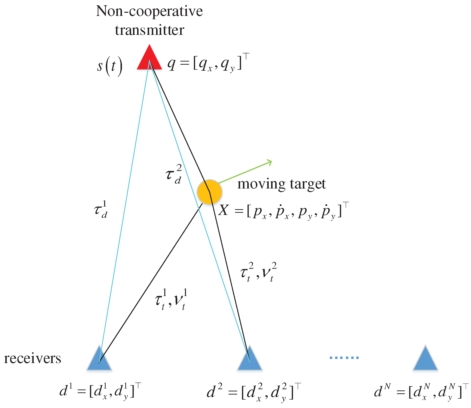
Suppose a PMR consisting of one non-cooperative transmitter of opportunity and N receivers is deployed to perform the DJDT of a target [26], as Figure 1 depicts. The two-dimensional position of the transmitter is denoted as $q={[q_x,q_y]}^{\top }$, the position of the j-th receiver is denoted as $d^j={[d_x^j,d_y^j]}^{\top }$, and the position and velocity of the moving target are denoted as $p={[p_x,p_y]}^{\top }$ and $\dot{p}={[{\dot{p}}_x,{\dot{p}}_y]}^{\top }$, respectively.

Suppose the target state is $X_k={[p_{x,k},{\dot{p}}_{x,k},p_{y,k},{\dot{p}}_{y,k}]}^{\top }$ at time step k, the evolution of $X_k$ is governed by the dynamic model

$$X_k=f_{k|k-1}\left(X_{k-1}\right)+v_{k-1},$$

(1)

where $f_{k|k-1}(·)$ is the transition function of X and $v_{k-1}$ is the Gaussian process noise.

The two directional receiving antennas point at the transmitter and the target echo, respectively, constructing the direct path and target path. The delay from the transmitter to the j-th receiver in the target path and direct path can be defined as ${\tau }_t^j=(\parallel p-q\parallel +\parallel d^j-p\parallel )/c$ and ${\tau }_d^j=\parallel d^j-q\parallel /c$, and the related Doppler in the two paths as ${\nu }_t^j=-f_c·({\dot{p}}^{\top }(p-q)/\parallel p-q\parallel +{(-\dot{p})}^{\top }(d^j-p)/\parallel d^j-p\parallel )/c$ in the line-of-sight cases and 0 Hertz, respectively, where c is the speed of wave propagation, $\parallel ·\parallel$ is the Euclidean norm, ${(·)}^{\top }$ is the transpose operator, and $f_c$ is the carrier frequency.

If the observation time lasts T seconds at each iteration, the received signals from the transmitter to the j-th receiver containing the surveillance signal and reference signal are:

$$\begin{array}{cc}\hfill z_s^j\left(t\right)& ={\alpha }^{j}s(t-{\tau }_t^j)e^{\iota 2\pi {\nu }_t^{j}t}+n_s^j\left(t\right),0\le t<T\hfill \\ \hfill z_r^j\left(t\right)& ={\beta }^{j}s(t-{\tau }_d^j)+n_r^j\left(t\right),\hfill \end{array}$$

(2)

where ${\alpha }^j$ and ${\beta }^j$ are unknown channel coefficients in the j-th surveillance-reference channel, respectively; ${\tau }_t^j,{\tau }_d^j\ll T$; $\iota$ is the imaginary unit; $s\left(t\right)$ is the unknown emitted narrowband signal envelope.

Assume the received signal is down-converted to the baseband and sampled at a rate of $f_s\gg B$ [9], discretizing the signals into vectors of length $L=f_{s}T$, the received waveforms in the j-th channel can, thus, be expressed as:

$$\begin{array}{cc}\hfill z_{s,k}^j& ={\alpha }_k^j\mathcal{D}({\tau }_{t,k}^j,{\nu }_{t,k}^j)·s_k+n_{s,k}^j,\hfill \\ \hfill z_{r,k}^j& ={\beta }_k^j\mathcal{D}({\tau }_{d,k}^j,0)·s_k+n_{r,k}^j,\hfill \end{array}$$

(3)

where $\mathcal{D}(\tau ,\nu )\in {\mathbb{C}}^{L\times L}$ is the unitary delay-Doppler operator that accounts for the delay and Doppler shift affecting the transmitted signal of length L as it propagates to the j-th receiver, given as

$$\mathcal{D}(\tau ,\nu )=D(\nu /f_s)W^{\mathrm{H}}D(\tau f_s/L)W,$$

(4)

where $D\left(u\right)=diag\left\{\left[e^{\iota 2\pi u·0,\cdots ,\iota 2\pi u·(L-1)}\right]\right\}$, where $diag\left\{[b_1,\cdots ,b_M]\right\}$ means the diagonal matrix with $b_1,\cdots ,b_M$ on the main diagonal. The superscript ${(·)}^{\mathrm{H}}$ is the conjugate transpose operator; $W\in {\mathbb{C}}^{L\times L}$ is the unitary discrete Fourier transform matrix, with its $(m,n)$-th element ${\left[W\right]}_{m,n}=\frac{1}{\sqrt{L}}{e}^{-\iota 2\pi mn/L},m,n=0,\cdots ,L-1$, where ${[·]}_{m,n}$ means the $(m,n)$-th entry of the matrix; $W^{\mathrm{H}}W=I_L$, thus $\mathcal{D}{(\tau ,\nu )}^{\mathrm{H}}\mathcal{D}(\tau ,\nu )=I_L$, where $I_M$ denotes $M\times M$ the identity of the matrix. $s_k\in {\mathbb{C}}^{L\times 1}$ denotes the sampled emitted signal, assuming that ${\parallel s_k\parallel }^2=L$; $n_{s,k}^j$ and $n_{r,k}^j\in {\mathbb{C}}^{L\times 1}$ are circular with zero-mean complex Gaussian noise and identical variance ${\sigma }_z^2$ and covariance $R_k={\sigma }_z^2{I}_L$, and are assumed independent across receivers and time intervals, i.e., $n_p^j{\left(n_q^n\right)}^{\mathrm{H}}={\sigma }_z^2{\delta }_{p-q}{\delta }_{j-n}{I}_L$, ${\delta }_b$ is the Dirac-delta function concentrated at point b. The signal vector is uncorrelated with the noise vectors since ${\alpha }_k^j$ and ${\beta }_k^j$ can be regarded as the scaling of the received signal; define SNR for the target-path as ${\mathrm{SNR}}^j=10lg({\left({\alpha }_k^j\right)}^2/{\sigma }_z^2)$ and for direct-path as ${\mathrm{DNR}}^j=10lg({\left({\beta }_k^j\right)}^2/{\sigma }_z^2)$.

For an explicit description, the concatenation of the surveillance signal and a reference signal to the j-th receiver can be defined as: $z_k^j={[{\left(z_{s,k}^j\right)}^{\top },{\left(z_{r,k}^j\right)}^{\top }]}^{\top }$, and the measurement vector gathering all the data as $z_k={[{\left(z_{s,k}^1\right)}^{\top },\cdots ,{\left(z_{s,k}^N\right)}^{\top },{\left(z_{r,k}^1\right)}^{\top },\cdots ,{\left(z_{r,k}^N\right)}^{\top }]}^{\top }$.

The same occurs as the binary hypothesis test between the alternative $\left(H_1\right)$ and null $\left(H_0\right)$ hypotheses; in the detection context, [9], the measurement vectors captured by the j-th receiver yield:

$$\begin{array}{cc}\hfill H_1:& z_{s,k}^j={\alpha }_k^j\mathcal{D}({\tau }_{t,k}^j,{\nu }_{t,k}^j)·s_k+n_{s,k}^j\hfill \end{array}$$

$$\begin{array}{cc}\hfill & z_{r,k}^j={\beta }_k^j\mathcal{D}({\tau }_{d,k}^j,0)·s_k+n_{r,k}^j,\hfill \\ \hfill H_0:& z_{s,k}^j=n_{s,k}^j\hfill \end{array}$$

(5)

$$\begin{array}{cc}\hfill & z_{r,k}^j={\beta }_k^j\mathcal{D}({\tau }_{d,k}^j,0)·s_k+n_{r,k}^j,\hfill \end{array}$$

(6)

in the two cases.

For ease of notation, we will abbreviate $\mathcal{D}({\tau }_{t,k}^j,{\nu }_{t,k}^j)$ as ${\mathcal{D}}_{t,k}^j$ and $\mathcal{D}({\tau }_{d,k}^j,0)$ as ${\mathcal{D}}_{d,k}^j$, which implicitly expresses full information associated with the target state, to adaptively generate the likelihood function for the PMR received signals.

3. The Proposed Method

3.1. The CAF-Based Likelihood

Construct $Q_k={\left({\Phi }_k\right)}^{\mathrm{H}}{\Phi }_k$ as the Gram matrix formed by the inner product of the delay-Doppler compensated surveillance and reference signals ([24], Equation (178)), where

$${\Phi }_k=[{\left({\mathcal{D}}_{t,k}^1\right)}^{\mathrm{H}}{z}_{s,k}^1,\cdots ,{\left({\mathcal{D}}_{t,k}^N\right)}^{\mathrm{H}}{z}_{s,k}^N,{\left({\mathcal{D}}_{d,k}^1\right)}^{\mathrm{H}}{z}_{r,k}^1,\cdots ,{\left({\mathcal{D}}_{d,k}^N\right)}^{\mathrm{H}}{z}_{r,k}^N].$$

(7)

For the convenience of identification, define ${\mathcal{D}}_{p,k}^j$ as the delay-Doppler operator, substituting the hypothesized target state, and ${\mathcal{D}}_{t,k}^j$ and ${\mathcal{D}}_{d,k}^j$ as the operator with the true target state. Replacing ${\mathcal{D}}_{t,k}^j$ with ${\mathcal{D}}_{p,k}^j$, we have

$${\Phi }_k=[{\left({\mathcal{D}}_{p,k}^1\right)}^{\mathrm{H}}{z}_{s,k}^1,\cdots ,{\left({\mathcal{D}}_{p,k}^N\right)}^{\mathrm{H}}{z}_{s,k}^N,{\left({\mathcal{D}}_{d,k}^1\right)}^{\mathrm{H}}{z}_{r,k}^1,\cdots ,{\left({\mathcal{D}}_{d,k}^N\right)}^{\mathrm{H}}{z}_{r,k}^N].$$

(8)

Since ${\left({\mathcal{D}}_{(p,d),k}^j\right)}^{\mathrm{H}}{z}_{(s,r),k}^j$ has the significance of shifting the measurement in time and frequency by ${\tau }_{(p,d)}^j$ and ${\nu }_{(p,d)}^j$ respectively, where ${(·)}_{(a,b)}$ denotes either ${(·)}_a$ or ${(·)}_b$, $Q_k$ implies the correlation of the reference and surveillance signals with respect to $X_k$.

Therefore, each column of ${\left({\Phi }_k\right)}^{\mathrm{H}}$ is a one snapshot-sampling of it, and the columns are approximately independent, identically distributed, N-variate complex Gaussian random vectors. It is worth noting that the true Gram matrix is not available; $Q_k$ is the L samples’ estimate of it, and a larger L reduces the estimating error.

According to the earlier discussions in [27] and ([28], Equation (19)), we conclude that $Q_k$ is distributed as complex Wishart with L degrees of freedom ([28], Equation (29)).

$${\mathcal{W}}_N^{\mathbb{C}}(Q;L,V)=\frac{{\left|V\right|}^{-L}{\left|Q\right|}^{(L-N)}{e}^{-\mathrm{tr}\left({\left(\mathrm{V}\right)}^{-1}\mathrm{Q}\right)}}{{\Gamma }_N^{\mathbb{C}}\left[L\right]},$$

(9)

where V is the $N\times N$ symmetric positive-definite scale matrix, and it can be seen as the expectation of the matrix variable Q if it is formed by one snapshot of $\Phi$, L is the degrees of freedom, $|·|$ denotes the determinant of the matrix, and ${\Gamma }_N^{\mathbb{C}}[·]$ is the complex multivariate Gamma function defined as ([28], Equation (30)).

If considering $Q_k$ as the pseudo measurement, we will obtain the likelihood in the PMR system

$${\phi }_k\left(Q_k\right|\left\{x\right\})={\mathcal{W}}_N^{\mathbb{C}}(Q_k;L,V_{k,1})$$

(10)

when assuming the target exists and

$${\phi }_k\left(Q_k\right|\varphi )={\mathcal{W}}_N^{\mathbb{C}}(Q_k;L,V_{k,0})$$

(11)

when assuming the target disappears, where $V_{k,1}$ and $V_{k,0}$ are, respectively, calculated under the alternative hypothesis and null hypothesis.

Observe that the state variable is simultaneously contained in $Q_k$, $V_{k,1}$, and $V_{k,0}$, we employ the property of the CAF [29] so that when the hypothesized state equals its true value, each entry of the matrix $Q_k$ reaches its maximum and the effect of $X_k$ in $V_{k,1}$ and $V_{k,0}$ is counteracted. It makes no sense to calculate $V_{k,1}$ and $V_{k,0}$ unless in the certain situation of ${\mathcal{D}}_{p,k}^j={\mathcal{D}}_{t,k}^j,j=1,\cdots ,N$. The certain value of $V_{k,1}$ and $V_{k,0}$ can be acquired by the following steps. First, substitute the measurement Function (5) or (6) for the two hypotheses into $Q_k$. Then, use the aforementioned assumption that the noise across the receivers are uncorrelated and the radiated signals and the noise is uncorrelated and withdraw the zero terms. Finally, assume the kinematic state is in the correct value, which is the specific condition we adopted.

Furthermore, the expected value of it, considering the statistic property of the random variables, can then be acquired. To this end, let us first compute $V_{k,1}$ as follows.

$$\begin{array}{cc}\hfill V_{k,1}& =\mathrm{E}\left\{{\left[{\left({\Phi }_k\right)}^{\mathrm{H}}\right]}_{ϵ}{\left[{\left({\Phi }_k\right)}^{\mathrm{H}}\right]}_{ϵ}^{\mathrm{H}}\right\}{|}_{{\mathcal{D}}_{p,k}^j={\mathcal{D}}_{t,k}^j,j=1,\cdots ,N}\hfill \\ \hfill & =\mathrm{E}{\left.\left\{{\left[\begin{array}{c}{\left(z_{s,k}^1\right)}^{\mathrm{H}}{\mathcal{D}}_{p,k}^1\\ ⋮\\ {\left(z_{s,k}^N\right)}^{\mathrm{H}}{\mathcal{D}}_{p,k}^N\\ {\left(z_{r,k}^1\right)}^{\mathrm{H}}{\mathcal{D}}_{d,k}^1\\ \begin{array}{c}⋮\\ {\left(z_{r,k}^N\right)}^{\mathrm{H}}{\mathcal{D}}_{d,k}^N\end{array}\end{array}\right]}_{ϵ}{\left[\begin{array}{c}{\left(z_{s,k}^1\right)}^{\mathrm{H}}{\mathcal{D}}_{p,k}^1\\ ⋮\\ {\left(z_{s,k}^N\right)}^{\mathrm{H}}{\mathcal{D}}_{p,k}^N\\ {\left(z_{r,k}^1\right)}^{\mathrm{H}}{\mathcal{D}}_{d,k}^1\\ \begin{array}{c}⋮\\ {\left(z_{r,k}^N\right)}^{\mathrm{H}}{\mathcal{D}}_{d,k}^N\end{array}\end{array}\right]}_{ϵ}^{\mathrm{H}}\right\}\right|}_{{\mathcal{D}}_{p,k}^j={\mathcal{D}}_{t,k}^j,j=1,\cdots ,N}\hfill \\ \hfill & =\mathrm{E}\left\{{\left[\begin{array}{c}{\alpha }_k^1\hfill \\ ⋮\hfill \\ {\alpha }_k^N\hfill \\ {\beta }_k^1\hfill \\ ⋮\hfill \\ {\beta }_k^N\hfill \end{array}\right]}^{*}{\left[\begin{array}{c}{\alpha }_k^1\hfill \\ ⋮\hfill \\ {\alpha }_k^N\hfill \\ {\beta }_k^1\hfill \\ ⋮\hfill \\ {\beta }_k^N\hfill \end{array}\right]}^{\top }\right\}+{\sigma }_z^2{I}_{2N}\hfill \\ \hfill & \approx {\left[\begin{array}{c}{\alpha }_k^1\hfill \\ ⋮\hfill \\ {\alpha }_k^N\hfill \\ {\beta }_k^1\hfill \\ ⋮\hfill \\ {\beta }_k^N\hfill \end{array}\right]}^{*}{\left[\begin{array}{c}{\alpha }_k^1\hfill \\ ⋮\hfill \\ {\alpha }_k^N\hfill \\ {\beta }_k^1\hfill \\ ⋮\hfill \\ {\beta }_k^N\hfill \end{array}\right]}^{\top }+{\sigma }_z^2{I}_{2N},\hfill \end{array}$$

(12)

where $\mathrm{E}\{·\}$ means the expectation, the superscript ${}^{*}$ denotes the complex conjugate, and ${[·]}_{ϵ}$ means the $ϵ$-th column of the matrix, or the $ϵ$-th element of the vector. Among the block matrix (12) calculation of each entry in the matrix block satisfying $r,u\le N$ can be detailed as:

$$\begin{array}{cc}\hfill & {\left[{\left({\alpha }_k^r{\mathcal{D}}_{t,k}^r{s}_k+n_{s,k}^r\right)}^{\mathrm{H}}{\mathcal{D}}_{p,k}^r\right]}_{ϵ}·{\left[{\left({\mathcal{D}}_{p,k}^u\right)}^{\mathrm{H}}\left({\alpha }_k^u{\mathcal{D}}_{t,k}^u{s}_k+n_{s,k}^u\right)\right]}_{ϵ}\hfill \\ \hfill & =({\left({\alpha }_k^r\right)}^{*}{\left(s_k\right)}^{\mathrm{H}}{\left({\mathcal{D}}_{t,k}^r\right)}^{\mathrm{H}}{\left[{\mathcal{D}}_{p,k}^r\right]}_{ϵ}+{\left(n_{s,k}^r\right)}^{\mathrm{H}}{\left[{\mathcal{D}}_{p,k}^r\right]}_{ϵ})·({\left[{\mathcal{D}}_{p,k}^u\right]}_{ϵ}^{\mathrm{H}}{\alpha }_k^u{\mathcal{D}}_{t,k}^u{s}_k+{\left[{\mathcal{D}}_{p,k}^u\right]}_{ϵ}^{\mathrm{H}}\left(n_{s,k}^u\right))\hfill \\ \hfill & =({\left({\alpha }_k^r\right)}^{*}{\left[s_k\right]}_{ϵ}^{\mathrm{H}}+{\left(n_{s,k}^r\right)}^{\mathrm{H}}{\left[{\mathcal{D}}_{p,k}^r\right]}_{ϵ})·({\alpha }_k^u{\left[s_k\right]}_{ϵ}+{\left[{\mathcal{D}}_{p,k}^u\right]}_{ϵ}^{\mathrm{H}}\left(n_{s,k}^u\right))\hfill \\ \hfill & ={\left({\alpha }_k^r\right)}^{*}{\left[s_k\right]}_{ϵ}^{\mathrm{H}}{\left[s_k\right]}_{ϵ}{\alpha }_k^u+{\left[{\mathcal{D}}_{p,k}^u\right]}_{ϵ}^{\mathrm{H}}\left(n_{s,k}^u\right){\left(n_{s,k}^r\right)}^{\mathrm{H}}{\left[{\mathcal{D}}_{p,k}^r\right]}_{ϵ}\hfill \\ \hfill & =\left\{\begin{array}{cc}\hfill & {\left({\alpha }_k^r\right)}^{*}{\alpha }_k^u+{\sigma }_z^2,\mathrm{if}r=u\hfill \\ \hfill & {\left({\alpha }_k^r\right)}^{*}{\alpha }_k^u,\mathrm{if}r\ne u\hfill \end{array}\right..\hfill \end{array}$$

(13)

The other three blocks of $V_{k,1}$, satisfying $N\le r,u\le 2N$, can be derived in the same way. Likewise, $V_{k,0}$ for target disappearance, can be expressed as:

$$\begin{array}{cc}\hfill V_{k,0}& =\mathrm{E}\left\{{\left[{\left({\Phi }_k\right)}^{\mathrm{H}}\right]}_{ϵ}{\left[{\left({\Phi }_k\right)}^{\mathrm{H}}\right]}_{ϵ}^{\mathrm{H}}\right\}{|}_{{\mathcal{D}}_{p,k}^j={\mathcal{D}}_{t,k}^j,j=1,\cdots ,N}\hfill \\ \hfill & =\mathrm{E}{\left.\left\{{\left[\begin{array}{c}{\left(n_{s,k}^1\right)}^{\mathrm{H}}{\mathcal{D}}_{p,k}^1\\ ⋮\\ {\left(n_{s,k}^N\right)}^{\mathrm{H}}{\mathcal{D}}_{p,k}^N\\ {\left(n_{r,k}^1\right)}^{\mathrm{H}}{\mathcal{D}}_{d,k}^1\\ \begin{array}{c}⋮\\ {\left(n_{r,k}^N\right)}^{\mathrm{H}}{\mathcal{D}}_{d,k}^N\end{array}\end{array}\right]}_{ϵ}{\left[\begin{array}{c}{\left(n_{s,k}^1\right)}^{\mathrm{H}}{\mathcal{D}}_{p,k}^1\\ ⋮\\ {\left(n_{s,k}^N\right)}^{\mathrm{H}}{\mathcal{D}}_{p,k}^N\\ {\left(n_{r,k}^1\right)}^{\mathrm{H}}{\mathcal{D}}_{d,k}^1\\ \begin{array}{c}⋮\\ {\left(n_{r,k}^N\right)}^{\mathrm{H}}{\mathcal{D}}_{d,k}^N\end{array}\end{array}\right]}_{ϵ}^{\mathrm{H}}\right\}\right|}_{{\mathcal{D}}_{p,k}^j={\mathcal{D}}_{t,k}^j,j=1,\cdots ,N}\hfill \\ \hfill & ={\sigma }_z^2{I}_{2N}.\hfill \end{array}$$

(14)

Consequently, the likelihood is called the CAF-based likelihood.

3.2. Bernoulli Filter Based DJDT

In this subsection, the Bernoulli filter, as the Bayes-optimal filter for detection and tracking in the scenario that is known to contain at most a single target, is adopted to address the problem of DJDT ([30], Section 13.2). Due to the non-Gaussian and non-linear nature of the likelihood, Gaussian mixture methods are used commonly to implement the standard Bernoulli filter where it cannot be readily employed and instead particle methods are utilized ([30], Section 19.4.4). ([25], Section IV) has presented the Bernoulli solution and a particle implementation using an intensity measurement model without passing a detector. The Bernoulli filter-based DJDT using the CAF-based likelihood (Bernoulli-CAF-DJDT) is put forward as follows.

A Bernoulli RFS X’s probability density function (PDF) is uniquely described by an existence probability r and the probability that it has state x, $p\left(x\right)$, called the spatial probability density function (SPDF), given by [31]

$$f\left(X\right)=\left\{\begin{array}{cc}1-r,\hfill & \mathrm{if}X=\varphi \hfill \\ r·p\left(x\right),\hfill & \mathrm{if}X=\left\{x\right\}.\hfill \end{array}\right.$$

(15)

The particle implementation solves the tracking problem by approximating the SPDF $p\left(x\right)$ as a series of weighted particles ${\left\{{\omega }^{\left(l\right)},x^{\left(l\right)}\right\}}_{l=1}^N$. The proposed CAF-DJDT approach is summarized in Algorithm 1, wherein the Bernoulli parameters are propagated in the form of ${\pi }_k=\left\{r_k,{\left\{{\omega }_k^{\left(l\right)},x_k^{\left(l\right)}\right\}}_{l=1}^N\right\}$. If Gaussian birth is assumed to have an object birth density of $b_{k-1}\left(x\right)$, then the transition density (1) is used as the proposal density.

Knowing the prior existence probability $r_{k-1}$ and SPDF ${\left\{{\omega }_{k-1}^{\left(l\right)},x_{k-1}^{\left(l\right)}\right\}}_{l=1}^N$, the prediction equations are listed in lines 6–7, where $P_s$ is the probability so that, if the target has the state x, it will survive, and $P_b$ is the probability that the target birth will appear in the scene. Provided that we have the predicted existence probability $r_{k|k-1}$, and the predicted SPDF ${\left\{{\omega }_{k|k-1}^{\left(l\right)},x_{k|k-1}^{\left(l\right)}\right\}}_{l=1}^{N+B}$ at time k, given the measurement vector $z_k$, the updated existence probability and SPDF for the Bernoulli are listed in lines 13–14, respectively.  

Algorithm 1: The proposed Bernoulli-DJDT approach

The proposed DJDT algorithm jointly detects and tracks the target position directly without extracting the middle parameters in advance and utilizes full knowledge of PMR received signals and, thus, reduces miss detection, information loss, and signal processing noise. Besides, a priori knowledge of the reference path reduces the required SNR. This gains an apparent advantage over the traditional sequential detection and JDT processing methods.

Remark 1. 

In addition to the proposed likelihood, another possibility is to adopt the GLRT-based likelihood which can be easily obtained by extending the results of [21]. The derivation details of the GLRT-based likelihood for DJDT are detailed in Appendix A. Compared with the GLRT-based likelihood, the CAF-based likelihood does not depend on the MLEs of unknown signal $s_k$, but it does depend on the product of a combination of ${\alpha }_k^j$ and ${\beta }_k^j$. Anyway, ${\mathrm{DNR}}^j$ is usually known, and ${\alpha }_k^j$ can be iteratively estimated by augmenting it into the target state; hence, the CAF-based likelihood preserves more knowledge of direct measurements than the other. This suppresses measurement noise in the Bernoulli update step efficiently, and there is no need to calculate a threshold. Its advantage will be shown in the following simulations.

Remark 2. 

It can be recalled from the preceding results in Section 3.1 and Appendix A that either the GLRT-based likelihood or the CAF-based likelihood employs all the correlations between the reference and surveillance signal intra receivers (delay and Doppler), surveillance signals across receivers (time difference of arrival (TDOA) and frequency difference of arrival (FDOA)), and reference and surveillance signals across the receivers. The reference signals provide a varying degree of knowledge about the transmitted signals that depends on the relative energy of true signals. The influence will be reflected in fixing ${\mathrm{DNR}}^j$ while changing ${\mathrm{SNR}}^j$ in the numerical simulations.

4. Simulation

4.1. Simulated Scenario

In this section, we are going to assess the performance of the proposed algorithm via simulation experiments. Consider the transmitter located at ${q=[4100,\mathrm{15,000}]}^{\top }$m and three receivers located at $d^1={[0,-500]}^{\top }\mathrm{m}$, $d^2={[5000,-800]}^{\top }\mathrm{m}$, and $d^3=[10$,000${,-500]}^{\top }\mathrm{m}$, respectively. A target moves with uniform speed along a straight-line path [32]. The target appears or disappears from the [0,10,000] $\mathrm{m}\times [-2000,$ 16,000] m surveillance volume, and it enters and leaves the scene at times 10 s and 80 s, respectively. The initial location and speed of the target are set by: ${[0\mathrm{m},105\mathrm{m}/\mathrm{s},0\mathrm{m},170\mathrm{m}/\mathrm{s}]}^{\top }$. Thus (1) becomes the nearly constant velocity model [33]

$$X_k=F{X}_{k-1}+v_{k-1},$$

(16)

with

$$F=\left[\begin{array}{cccc}1& \Delta & 0& 0\\ 0& 1& 0& 0\\ 0& 0& 1& \Delta \\ 0& 0& 0& 1\end{array}\right],W_{k-1}={\sigma }_v^2\left[\begin{array}{cccc}{\Delta }^4/3& {\Delta }^3/2& 0& 0\\ {\Delta }^3/2& {\Delta }^2& 0& 0\\ 0& 0& {\Delta }^4/3& {\Delta }^3/2\\ 0& 0& {\Delta }^3/2& {\Delta }^2\end{array}\right],$$

(17)

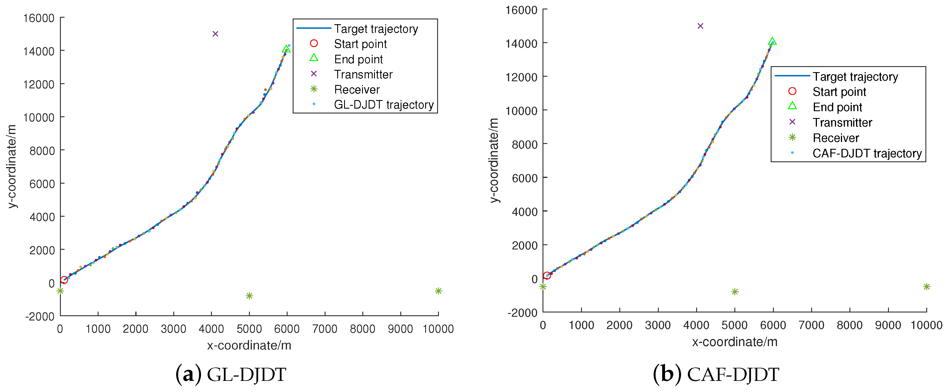
where F denotes the linear transition matrix with $\Delta$ representing the sampling time interval, and $v_{k-1}$ has the covariance matrix $W_{k-1}$ and the standard deviation ${\sigma }_v=15\mathrm{m}/{\mathrm{s}}^2$. The topology of the transmitter, receivers, and target trajectory is shown in Figure 2a.

The measurement model has been shown in (3), where the PMR parameters are the signal observation time $T=1$ ms, $f_c=540$ MHz, $c=3\times {10}^8$ m/s, and the transmitted signal is simply represented by a binary phase shift keying (BPSK) signal: $s\left(t\right)=e^{\iota (2\pi f_{c}t+\eta \left(t\right))}$, where $\eta \left(t\right)$ is the symbol with a symbol rate of $1\times {10}^5$ symbol/s. As the final results of Section 3 reveals the tracking precision does not depend on the specific structure of the signal waveform but on the power of the signal. Each logarithmic surveillance channel coefficient $ln{\alpha }_k^j,\forall j$ is modeled as a random variable that conforms to Gaussian distribution with zero mean and standard deviation $0.02$ and ${\sigma }_z$ which is calculated by the common SNR of the surveillance signals. In the following simulations, without loss of generality, all the ${\mathrm{DNR}}^j,\forall j$ are fixed at 10 dB. To be more computationally effective, we processed the baseband signal and $L=100$ snapshots were gathered.

The initial state and covariance matrix are set as follows

$$X_0={[0,0,0,0]}^{\top },P_0={\left[\begin{array}{cccc}100& 0& 0& 0\\ 0& 100& 0& 0\\ 0& 0& 100& 0\\ 0& 0& 0& 100\end{array}\right]}^2.$$

(18)

The birth model is Gaussian with mean ${[0,0,0,0]}^{\top }$ on the position and velocity dimension and $P_b=0.01$.

For CAF-DJDT, in order to estimate the channel coefficients and kinematic state together, the state vector should be extended to $X_k={[p_{x,k},{\dot{p}}_{x,k},p_{y,k},{\dot{p}}_{y,k},ln{\alpha }_k^1,ln{\alpha }_k^2,ln{\alpha }_k^3]}^{\top }$, the transition matrix and noise covariance matrix are changed to

$$F^{\prime }=diag\{F,I_3\},W_{k-1}^{\prime }=diag\{W_{k-1},{\sigma }_{ln\alpha }^2{I}_3\},$$

(19)

respectively, where the $diag\{·\}$ represents the block diagonal matrix and ${\sigma }_{ln\alpha }=0.05$. The receivers collected 100 scans in total and 100 Monte Carlo trials were carried out to evaluate the experiments. The GL-DJDT can also be implemented by the offered Bernoulli filter (Bernoulli-GL-DJDT). We used 1500 particles to approximate the target survival and 500 particles to approximate the object birth for GL-DJDT and 4000 particles to approximate the target survival, and 900 particles to approximate the object birth for CAF-DJDT. Please note that to the GL-DJDT, there is no reliable way of calculating the pseudo threshold $\gamma$. Fortunately, we only needed the about value of it with the proposed Monte-Carlo method.

4.2. Results

To better illustrate Bernoulli-CAF-DJDT’s superiority, we also performed a typical traditional two-step PMR surveillance method under the same background and settings for comparison. Step 1 is to extract the delay and Doppler, which is implemented by a two-dimensional grid search to find the maximum CAF for each transmitter-receiver channel pair [9]. $f_s$ is set to $2\mathrm{MHz}$ and the grid size is $1/f_s$ = 0.125 μs and 1 Hz for the delay and Doppler, respectively, to determine the parameter resolution. The second step is a common particle-based Bernoulli filter ([25], Algorithm 2) with the standard deviation of the measurement noise, which is determined by the time-averaged root mean squared errors (RMSEs) of the estimated delays and Dopplers, i.e.,

$${\sigma }_{\tau }^j={\mathrm{RMSE}}_{\tau }^j=\sqrt{\frac{1}{100}\sum _{k=1}^{100}{\left({\tau }_k^j-\mathrm{E}\left\{{\tau }_k^j\right\}\right)}^2},{\sigma }_{\nu }^j={\mathrm{RMSE}}_{\nu }^j=\sqrt{\frac{1}{100}\sum _{k=1}^{100}{\left({\nu }_k^j-\mathrm{E}\left\{{\nu }_k^j\right\}\right)}^2}$$

(20)

for $j=1,\cdots ,N$. They are in a positive correlation with SNR. The surveillance region is in the best condition with one clutter returning over the volume, and the detection probability is $p_d=0.99$. A total of 1000 snapshots were gathered since fewer snapshots resulted in the OSPA exceeding 80 m, which is not necessary to exhibit in the figure.

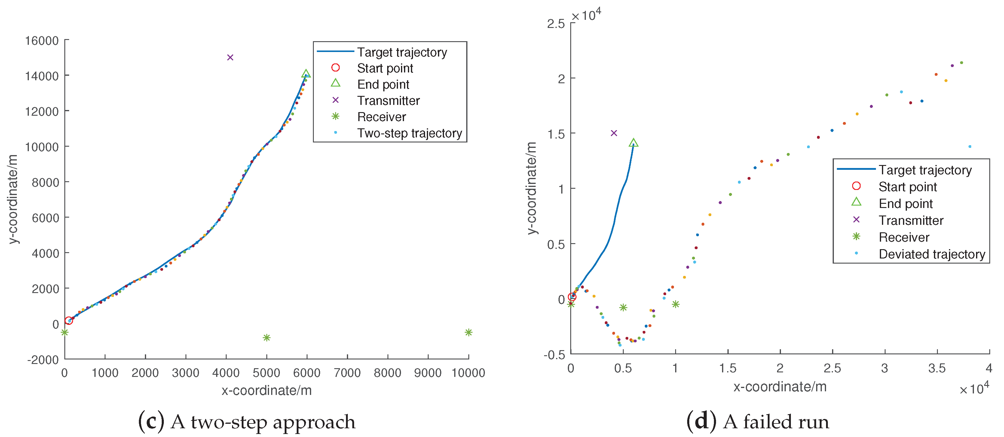
To begin with, Figure 2a–c depicts the estimated trajectory of a typical run with the GL-DJDT/ CAF-DJDT Bernoulli filter under $\mathrm{SNR}=-12$ dB and the two-step approach under $\mathrm{SNR}=10$ dB, respectively. The logarithmic scale of the SNR-dependent threshold $\in \gamma$ is calculated approximately as 10. As can be seen qualitatively from Figure 2a–c, all the given methods have correctly performed DJDT, and the two-step method does not work as well as them.

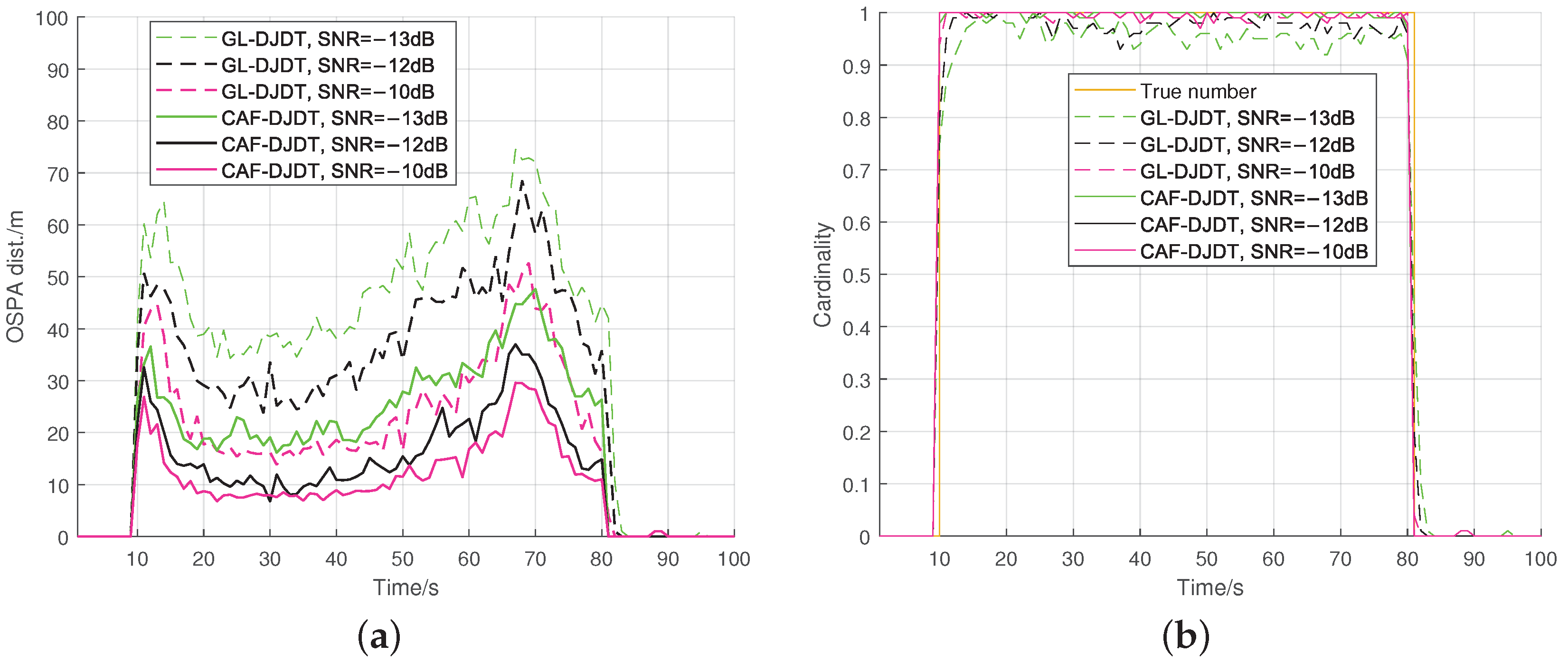
To show that the proposed method works well in varied noise levels explicitly, Figure 3a exhibits the optimal sub-patterns (OSPAs) with order $p=1$ and cutoff $c=100$ on the target position under $\mathrm{SNR}=-13,-12,-10$ dB for the Bernoulli-GL-DJDT and Bernoulli-CAF-DJDT versus time k. The corresponding $ln\gamma$ is calculated as 9, 10, and 13. During experiments, when SNR is lower than −13 dB for the Bernoullli-GL-DJDT and the Bernoullli-CAF-DJDT, the track may seriously deviate from its true trajectory in some Monte–Carlo runs, see Figure 2d. Figure 3a confirms Remark 1 in that GL-DJDT exhibits higher OSPA errors in the environment of the same SNR, especially in low SNR environments ($\mathrm{SNR}\le -12$ dB). Additionally, more false alarms appeared at the end of the trajectory (81 s) when $\mathrm{SNR}\le -12$ dB. This is because the existence probability could not drop quickly once the likelihood ratio dropped. Summarily, the CAF-DJDT is 3 dB better than the GL-DJDT within the normal operating range of $\mathrm{SNR}\ge -13$ dB.

The OSPA distance simultaneously captures the cardinality error and state error. We present the detection performance separately by plotting the time-varying cardinality in Figure 3b. The ground truth cardinality is illustrated by the khaki line as well. We can draw conclusions that the OSPA errors mostly result from the estimation bias in the number of targets and miss detections which becomes severe as noise become louder. In addition, the performance of Bernoulli-GL-DJDT is inferior to the proposed method.

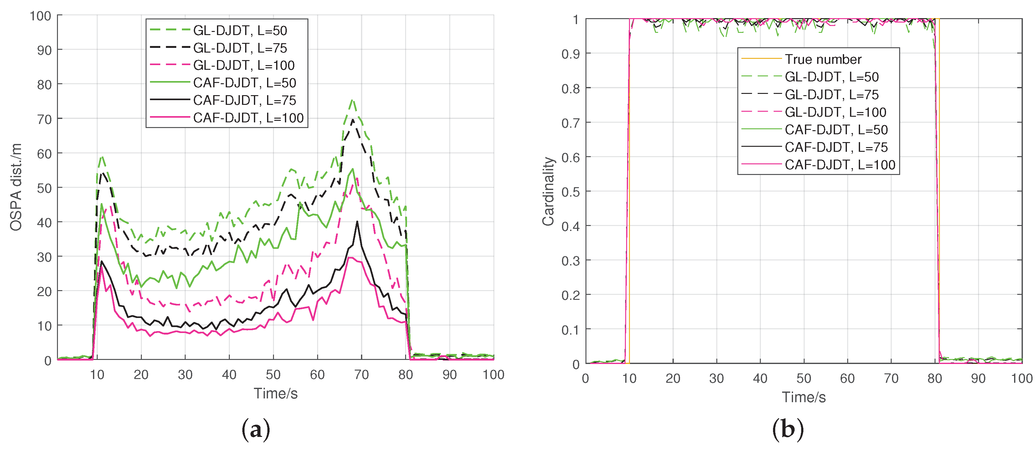
Analogously, the results are summarized in Figure 4a, which illustrates OSPA errors and the cardinality of the two DJDT methods versus time steps with the number of snapshots $L=50,75,100$ with SNR = −10 dB. It can be easily concluded that the proposed method shows lower errors and more robustness to noise compared to the Bernoulli-GL-DJDT approach in all the two different parameter settings. The superior performance of the proposed method compared to the Bernoulli-GL-DJDT approach is mainly due to the correlation of the reference and surveillance signals. However, due to a lack of correlation information, the two DJDT methods cannot work with $L\le 50$ and SNR = −10 dB.

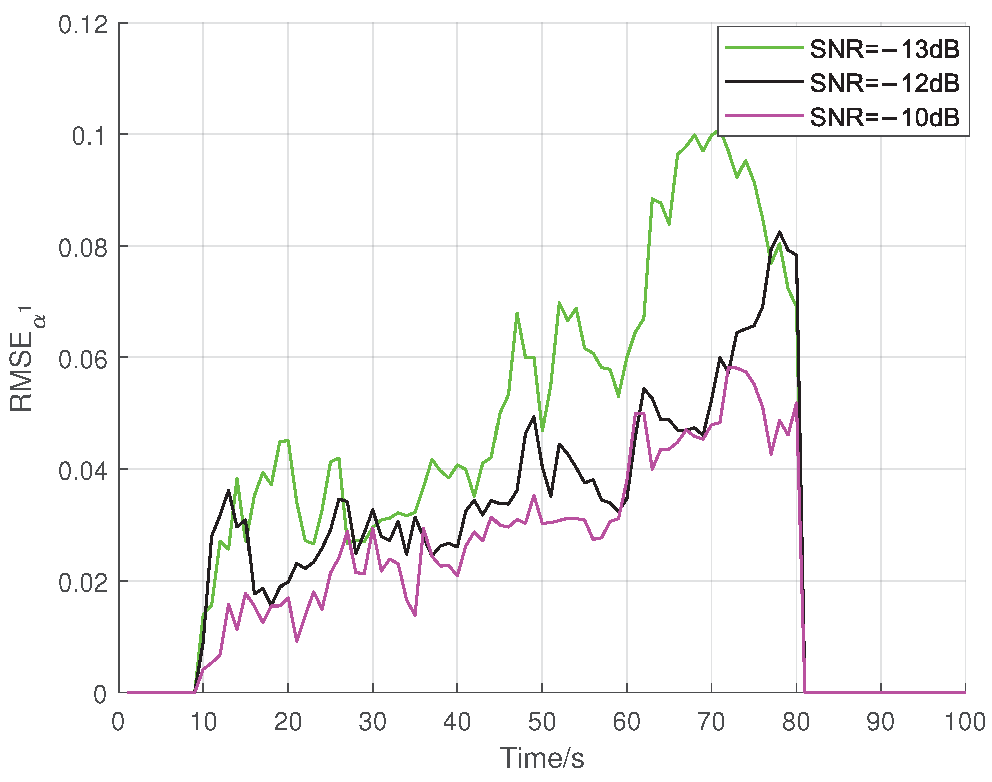
The error of the estimated time-varying ${\alpha }_k^j$ is reflected by the RMSE of ${\alpha }_k^1$ for the first receiver. The results versus time from 10 s to 80 s are shown in Figure 5 with $\mathrm{SNR}=-13,-12,$ and $-10$ dB. The errors in the latter half of the period rise and gradually converge. This can be interpreted by the topology of the track, transmitter, and receivers becoming harder to observe.

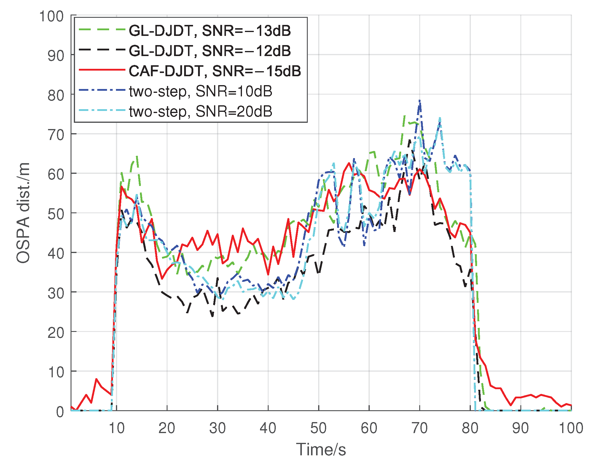
Furthermore, to show the performance improvements in the whole PMR signal processing flow, Figure 6 exhibits the OSPAs for the Bernoullli-GL-DJDT on condition of $\mathrm{SNR}=-13,-12$ dB, and Bernoullli-CAF-DJDT on condition of $\mathrm{SNR}=-15$ dB and the two-step approach under the condition of $\mathrm{SNR}=10,20$ dB versus time. And the standard deviation of the delay and Doppler are respectively computed around ${\sigma }_{\tau }=4.63\times {10}^{-8}\sim 6.47\times {10}^{-8}$ s and ${\sigma }_{\nu }=24.29\sim 31.50$ Hz under $\mathrm{SNR}=10,20$ dB. On the one hand, in the given environments, the two DJDT and the two-step approach lead to similar OSPA levels, while the OSPAs of the two-step approach is unstable and prone to divergence. On the other hand, CAF-DJDT under $\mathrm{SNR}=-15$ dB exhibits some overestimates in the target number during target absent time, which is due to the useful signals submerging in noise and the likelihood not being able to tell the difference between measurements with or without a target. Anyway, the SNR is adequate for practical use, and lower SNR can be achieved by making use of more particles and more snapshots. In addition, the two-step approach results in similar OSPA levels under $\mathrm{SNR}=10$ and 20 dB, and it seems insensitive to the change of SNR [18]. The cause is that the performance of two-step tracking mostly depends on the accuracy of parameter estimates produced by step 1, which displays fluctuations when finding the peak and when it does not. In contrast to the conventional method, the proposed DJDT approach could produce more accurate position estimates at the beginning of the trajectory and maintain stability since it preserves the information of the raw data. Specifically, the Bernoulli-GL-DJDT raises the SNR by 22∼33 dB, and the Bernoulli-CAF-DJDT raises the SNR by 25∼35 dB.

Finally, to compare the computation load of algorithms,

Table 1. Execution time per trial.

Algorithm	Time [s]
Bernoulli GL-DJDT	141.2
Bernoulli CAF-DJDT	150.3
Bernoulli two-step method	124.0

prints the MATLAB processing time for one Monte–Carlo trail for all the considered methods. The runtime indicates that the computation burden of the two DJDT methods is almost equal. The CAF-DJDT gains a tracking performance at the expense of computation.

5. Conclusions

This paper is devoted to the problem of DJDT using a set of received signals in a PMR system. A novel likelihood is developed on the basis of the delay-Doppler compensated surveillance and reference signals’ Gram matrix by approximating the distribution of it in a certain circumstance. The tracking framework is implemented by a modified Bernoulli filter based on particle approximations. Compared with the approach of generalizing the original likelihood to the MLE of it, and the traditional two-step PMR tracking approach, the proposed Bernoulli-CAF-DJDT filter reduces error accumulation and exhibits significant improvements in both location estimates and detection performance. The effectiveness of the algorithm has been validated through reasonable simulations. Possible future work will concern the problem of multi-target direct tracking.

References

- Griffiths, H.D.; Baker, C.J. An Introduction to Passive Radar; Artech House: Norwood, MA, USA, 2022. [Google Scholar]
- Baker, C.; Griffiths, H.; Papoutsis, I. Passive coherent location radar systems. Part 2: Waveform properties. IEE Proc. Radar Sonar Navig. 2005, 152, 160–168. [Google Scholar] [CrossRef]
- ATSC-A/153; ATSC-Mobile Television Standard, Part 2-RF/Transmission System Characteristics. Advanced Television Systems Committee, Inc.: Washington, DC, USA, 2011.
- Tan, D.K.; Sun, H.; Lu, Y.; Lesturgie, M.; Chan, H.L. Passive radar using global system for mobile communication signal: Theory, implementation and measurements. IEE Proc. Radar Sonar Navig. 2005, 152, 116–123. [Google Scholar] [CrossRef]
- Kuschel, H.; Heckenbach, J.; Muller, S.; Appel, R. On the potentials of passive, multistatic, low frequency radars to counter stealth and detect low flying targets. In Proceedings of the 2008 IEEE Radar Conference, Rome, Italy, 26–30 May 2008; pp. 1–6. [Google Scholar]
- Robey, F.; Fuhrmann, D.; Kelly, E.; Nitzberg, R. A CFAR adaptive matched filter detector. IEEE Trans. Aerosp. Electron. Syst. 1992, 28, 208–216. [Google Scholar] [CrossRef] [Green Version]
- Klein, M.; Millet, N. Multireceiver passive radar tracking. IEEE Aerosp. Electron. Syst. Mag. 2012, 27, 26–36. [Google Scholar] [CrossRef]
- Daun, M.; Koch, W. Multistatic target tracking for non-cooperative illuminating by DAB/DVB-T. In Proceedings of the OCEANS 2007—Europe, Aberdeen, UK, 18–21 June 2007; pp. 1–6. [Google Scholar]
- Hack, D.E.; Patton, L.K.; Himed, B.; Saville, M.A. Detection in Passive MIMO Radar Networks. IEEE Trans. Signal Process. 2014, 62, 2999–3012. [Google Scholar] [CrossRef]
- Hack, D.E.; Patton, L.K.; Himed, B.; Saville, M.A. Centralized Passive MIMO Radar Detection Without Direct-Path Reference Signals. IEEE Trans. Signal Process. 2014, 62, 3013–3023. [Google Scholar]
- Jauffret, C.; Bar-Shalom, Y. Track formation with bearing and frequency measurements in clutter. IEEE Trans. Aerosp. Electron. Syst. 1990, 26, 999–1010. [Google Scholar] [CrossRef]
- Malanowski, M.; Kulpa, K.; Suchozebrski, R. Two-stage tracking algorithm for passive radar. In Proceedings of the 2009 12th International Conference on Information Fusion, Seattle, WA, USA, 6–9 July 2009; pp. 1800–1806. [Google Scholar]
- Bozdogan, A.O.; Soysal, G.; Efe, M. Multistatic tracking using bistatic range-Range rate measurements. In Proceedings of the 2009 12th International Conference on Information Fusion, Seattle, WA, USA, 6–9 July 2009; pp. 2107–2113. [Google Scholar]
- So, H.; Ching, P.; Chan, Y. A new algorithm for explicit adaptation of time delay. IEEE Trans. Signal Process. 1994, 42, 1816–1820. [Google Scholar] [CrossRef]
- Amar, A.; Weiss, A.J. Localization of Narrowband Radio Emitters Based on Doppler Frequency Shifts. IEEE Trans. Signal Process. 2008, 56, 5500–5508. [Google Scholar] [CrossRef]
- Weiss, A.J. Direct Geolocation of Wideband Emitters Based on Delay and Doppler. IEEE Trans. Signal Process. 2011, 59, 2513–2521. [Google Scholar] [CrossRef]
- Vu, P.; Haimovich, A.M.; Himed, B. Direct tracking of multiple targets in MIMO radar. In Proceedings of the IEEE 2016 50th Asilomar Conference on Signals, Systems and Computers, Pacific Grove, CA, USA, 6–9 November 2016; pp. 1139–1143. [Google Scholar]
- Yin, X.; Pedersen, T.; Blattnig, P.; Jaquier, A.; Fleury, B.H. A single-stage target tracking algorithm for multistatic DVB-T passive radar systems. In Proceedings of the IEEE 13th Digital Signal Processing Workshop and 5th IEEE Signal Processing Education Workshop, Marco Island, FL, USA, 4–7 January 2009; pp. 518–523. [Google Scholar]
- Sidi, A.Y.; Weiss, A.J. Delay and Doppler Induced Direct Tracking by Particle Filter. IEEE Trans. Aerosp Electron Syst. 2014, 50, 559–572. [Google Scholar] [CrossRef]
- Sun, M.; Xia, W.; Wang, Y. Direct Target Tracking by Distributed Gaussian Particle Filtering Based on Delay and Doppler. In Proceedings of the 14th IEEE International Conference on Signal Processing, Beijing, China, 12–16 August 2018; pp. 58–63. [Google Scholar]
- Xia, W.; Sun, M.; Wang, Q. Direct Target Tracking by Distributed Gaussian Particle Filtering for Heterogeneous Networks. IEEE Trans. Signal Process. 2020, 68, 1361–1373. [Google Scholar] [CrossRef]
- Chen, Y.; Wei, P.; Li, G.; Zhang, H.; Liao, H. Emitter Tracking via Direct Target Motion Analysis. IEICE Trans. Fundam. Electron. Commun. Comput. Sci. 2022, E105.A, 1522–1536. [Google Scholar] [CrossRef]
- Liu, J.; Li, H.; Himed, B. Two Target Detection Algorithms for Passive Multistatic Radar. IEEE Trans. Signal Process. 2014, 62, 5930–5939. [Google Scholar] [CrossRef]
- Hack, D.E. Passive MIMO Radar Detection; Air Force Institute of Technology: Wright-Patterson Air Force Base, OH, USA, 2013. [Google Scholar]
- Ristic, B.; Vo, B.T.; Vo, B.N.; Farina, A. A tutorial on Bernoulli filters: Theory, implementation and applications. IEEE Trans. Signal Process. 2013, 61, 3406–3430. [Google Scholar] [CrossRef]
- Farina, A. Tracking function in bistatic and multistatic radar systems. IEE Proc. F Commun. Radar Signal Process. 1986, 133, 630. [Google Scholar] [CrossRef]
- Goodman, N.R. Statistical Analysis Based on a Certain Multivariate Complex Gaussian Distribution (An Introduction). Ann. Math. Stat. 1963, 34, 152–177. [Google Scholar] [CrossRef]
- Alireza, M.S.; Bhaskar, D.R. A Covariance-Based Superpositional CPHD Filter for Multisource DOA Tracking. IEEE Trans. Signal Process. 2018, 66, 309–323. [Google Scholar]
- Stein, S. Differential delay/Doppler ML estimation with unknown signals. IEEE Trans. Signal Process. 1993, 41, 2717–2719. [Google Scholar] [CrossRef]
- Mahler, R.P. Advances in Statistical Multisource-Multitarget Information Fusion; Artech House: Norwood, MA, USA, 2014. [Google Scholar]
- Vo, B.T.; See, C.M.; Ma, N.; Ng, W.T. Multi-sensor joint detection and tracking with the Bernoulli filter. IEEE Trans. Aerosp. Electron. Syst. 2012, 48, 1385–1402. [Google Scholar] [CrossRef]
- Choi, S.; Crouse, D.F.; Willett, P.; Zhou, S. Approaches to Cartesian Data Association Passive Radar Tracking in a DAB/DVB Network. IEEE Trans. Aerosp. Electron. Syst. 2014, 50, 649–663. [Google Scholar] [CrossRef]
- Boers, Y. Multitarget particle filter track before detect application. IEE Proc. Radar Sonar Navig. 2004, 151, 351–358. [Google Scholar] [CrossRef]
- Kelly, E. An Adaptive Detection Algorithm. IEEE Trans. Aerosp. Electron. Syst. 1986, AES-22, 115–127. [Google Scholar] [CrossRef] [Green Version]
- Kay, S.M.M. Fundamentals of Statistical Signal Processing, Vol. II: Detection Theory; Prentice Hall PTR: Upper Saddle River, NJ, USA, 1993. [Google Scholar]
- Bialkowski, K.S.; Clarkson, I.V.L.; Howard, S.D. Generalized canonical correlation for passive multistatic radar detection. In Proceedings of the 2011 IEEE Statistical Signal Processing Workshop (SSP), Nice, France, 28–30 June 2011; pp. 417–420. [Google Scholar]
- Horn, R.A.; Johnson, C.R. Matrix Analysis; Cambridge University Press: Cambridge, UK, 2012. [Google Scholar]
- Cui, G.; Liu, J.; Li, H.; Himed, B. Signal detection with noisy reference for passive sensing. Signal Process. 2015, 108, 389–399. [Google Scholar] [CrossRef]
- Fazlollahpoor, M.; Derakhtian, M.; Khorshidi, S. Rao Detector for Passive MIMO Radar With Direct-Path Interference. IEEE Trans. Aerosp. Electron. Syst. 2020, 56, 2999–3009. [Google Scholar] [CrossRef]
- De Maio, A. Rao Test for Adaptive Detection in Gaussian Interference With Unknown Covariance Matrix. IEEE Trans. Signal Process. 2007, 55, 3577–3584. [Google Scholar] [CrossRef]
Figure 1.
Typical deployment of a PMR.
Figure 2.
Simulated scenario and a typical Monte Carlo run.
Figure 3.
Comparision of two DJDT methods with different SNRs. (a) OSPA errors of two DJDT methods with different SNRs; (b) Cardinality of two DJDT methods with different SNRs.
Figure 4.
Comparision of two DJDT methods with a different number of snapshots. (a) OSPA errors of two DJDT methods with a different number of snapshots; (b) Cardinality of two DJDT methods with a different number of snapshots.
Figure 5.
RMSEs of the channel coefficient for the first receiver of the proposed method with different SNRs.
Figure 6.
OSPAs of considered methods with different SNRs.