


Evaluating the Value of CrIS Shortwave-Infrared Channels in Atmospheric-Sounding Retrievals

1
Science and Technology Corporation, Columbia, MD 21046, USA
2
Cooperative Institute for Satellite Earth System Studies, University of Maryland, College Park, MD 20742, USA
3
NOAA/NESDIS/STAR, College Park, MD 20740, USA
*
Author to whom correspondence should be addressed.
Remote Sens. 2023, 15(3), 547; https://doi.org/10.3390/rs15030547
Submission received: 18 November 2022
/
Revised: 6 January 2023
/
Accepted: 12 January 2023
/
Published: 17 January 2023
(This article belongs to the Special Issue Remote Sensing for the Improvement of High-Impact Weather Analyses and Forecasts)
Abstract
:The Cross-track Infrared Sounder (CrIS), in low Earth orbit since 2011, makes measurements of the top of atmosphere radiance for input into data assimilation (DA) systems as well as the retrieval of geophysical state variables. CrIS measurements have 2211 narrow infrared channels ranging between 650 and 2550 cm−1 (~3.9–15.4 μm) and capture the variation in profiles of atmospheric temperature, water vapor, and numerous trace gas species. DA systems derive atmospheric temperature by assimilating CO2-sensitive channels in the CrIS longwave (LW) band (650–1095 cm−1). Here, we investigate if CO2-sensitive channels in the shortwave (SW) band (2155–2550 cm−1) can similarly be applied. We first evaluated the information content of the CrIS bands followed by an assessment of the performance degradation of retrievals due to the loss of individual CrIS bands. We found that temperature profile retrievals derived from the CrIS SW band were statistically both well-behaved and as accurate as a retrieval utilizing the CrIS LW band. The one caveat, however, is that the higher CrIS instrument noise in the SW band limited its performance under certain conditions. We conclude with a discussion on the implications our results have for channel selection in retrieval and DA systems as well as the design of future space instruments.
1. Introduction
Our primary intent in this paper is to encourage the utilization of the shortwave (SW) band of existing space-borne infrared weather instruments and to provide guidance on whether future instruments could utilize the SW spectral region as a replacement for the more traditional LW spectral region in weather applications. Modern-era infrared (IR) sounders measure the top of atmosphere-emitted radiance in thousands of narrow channels from ~650 to ~2550 cm−1 (~3.9–15.4 μm). Instruments with such high spectral resolution have sensitivity to energy emitted by a host of atmospheric gases at many different pressure layers: first and foremost, water vapor (H2Ovap) and ozone (O3), and to a lesser extent, carbon monoxide (CO), carbon dioxide (CO2), methane (CH4), nitric acid (HNO3), sulfur dioxide (SO2), nitrogen oxide (N2O), and ammonia (NH3). Both data assimilation (DA) and retrieval systems employ Bayesian mathematics to derive parameters representing the atmospheric state. Numerical weather prediction (NWP) global DA systems utilize a large number of observational sources (i.e., numerous satellite and ground-based instruments) to simultaneously retrieve a diverse set of state variables on a uniform grid. Retrieval systems, on the other hand, utilize the information available from a single satellite along its line-of-sight to retrieve only those geophysical parameters for which that satellite is sensitive. Hyperspectral IR sounders have information about lower-, mid-, and upper atmospheric temperature in CO2-sensitive channels of the ~4.3 μm (~2300 cm−1) and ~15 μm (~660–700 cm−1) IR regions. Traditionally, only the longwave (LW) CO2 channels at ~15 μm have been used in DA systems [1] because they are insensitive to the daytime effects caused by solar reflectivity and non-Local Thermodynamic Equilibrium (non-LTE) [2,3]. With non-LTE mostly addressed by improvements in SW radiative transfer calculations [4,5], some Bayesian retrieval systems now include channels from the SW ~4.3 μm and LW ~15 μm CO2-sensitive bands in their temperature retrievals for added stability and sounding capability [6,7,8]. In this paper, we evaluate the potential of using CrIS SW CO2-sensitive channels as a possible replacement for the CrIS LW channels in order to understand the feasibility of smaller instruments that lack the ~15 μm CO2 IR absorption band [9].
The Cross-track Infrared Sounder (CrIS) [10,11], a Michelson interferometer, has been in low Earth orbit since 2011 when it was launched on the Suomi National Polar-orbiting Partnership (SNPP) platform. Soon after, the National Oceanic and Atmospheric Administration (NOAA) started to generate CrIS measurements and products operationally in support of weather forecast systems and applications. NOAA continues to do so for CrIS on the Joint Polar Satellite System (JPSS-1) platform that was launched in 2017 (operationally known as NOAA-20). Three additional CrIS instruments are scheduled for launch on JPSS satellites well into 2040. The 2211 full-spectral resolution CrIS channels can be grouped into three bands; LW (650.0–1095 cm−1 with 713 channels), midwave (MW; 1210–1750 cm−1 with 865 channels) and SW (2155–2550 cm−1 with 633 channels). Other hyperspectral sounders that utilize these spectral regions include the legacy Atmospheric Infrared Sounder (AIRS) on Aqua since 2002 [12] and the Infrared Atmospheric-Sounding Interferometer (IASI) [13] on a series of MetOp satellites since 2006. Table 1 in [7] summarizes and contrasts these three instruments.
With a record spanning more than two decades, there is strong evidence of the unique and valuable contribution spaceborne hyperspectral IR measurements make to NWP global DA systems [1,14,15,16,17,18,19,20,21,22,23,24]. Similarly, geophysical variables retrieved from hyperspectral IR measurements have value in real-time weather monitoring and forecasting [25,26,27,28,29,30]. In general, operational DA systems use small subsets of IR channels that are most sensitive to vertical profiles of atmospheric temperature (Tp) and water vapor (H2Ovap) [2]. The CrIS radiances should invoke changes in the background fields of Tp and H2Ovap but could also invoke changes in other background fields such as wind or height. Retrieval systems, on the other hand, are optimized to extract the maximum information from instruments aboard a specific satellite and they extract multiple atmospheric state variables, such as surface temperature, emissivity, cloud fraction, cloud top pressure, O3, CO, CH4, CO2, HNO3, N2O and a host of minor gases, in addition to Tp and H2Ovap. Some retrieval systems are statistical inversions that use all available IR channels [31,32,33,34,35]. Statistical retrievals can be implemented rapidly and require fewer operational resources. Other retrieval systems adopt Bayesian Optimal Estimation (O-E)—similar to the mathematics employed in DA—that require detailed radiative-transfer calculations that can consume resources. One way to speed up O-E computations is to utilize subsets of IR channels selected for each target variable [7,36,37,38]. There are various methods to use when selecting channels for a specific system or retrieval variable [15,19,39,40,41,42,43,44] and they all have in common the goal to reduce data volume for higher computational efficiency and to improve signal-to-noise for better stability across the globe under many types of weather conditions. Stability is achieved when inversion solutions converge without artifacts such as vertical oscillations or large errors in specific geographic regions or meteorological regimes.
Channels selected for assimilation in NWP global DA systems usually exclude the SW ~4.3 μm band in favor of the LW ~15 μm CO2 absorption band because the SW band is (i) subject to non-LTE effects that are historically difficult to model; (ii) sensitive to reflected solar irradiance, and (iii) subject to non-linear effects of the Planck function. Issues (i) and (iii) will be discussed in more detail in Section 2.2.1 and Section 2.2.2, respectively, and have been resolved in modern retrieval systems. For issue (ii), NUCAPS solves for spectral emissivity and spectral effective reflectivity (i.e., we allow for changes to the solar irradiance) and, as such, it is part of the NUCAPS state vector and error budget. In applications where the surface emissivity, reflectivity, and solar irradiance are assumed known, special care must be taken—especially over specular reflecting ocean and lake regions. Some daytime scenes may need to be ignored (i.e., glint conditions).
With new instrument designs that favor narrower spectral ranges for cost efficiency, e.g., the pathfinder CubeSat Infrared Atmospheric Sounder (CIRAS) [9,45,46], we revisit the work by [47] on SW IR capability and ask if CO2 channels in the LW (~15 μm) and SW (~4.3 μm) absorption regions can be functionally equivalent. Our research question is this: “Can atmospheric temperature be retrieved with the same quality and stability using CO2 sensitive channels centered at ~4.3 μm and ~15 μm, respectively?”
We address this question using an off-line version of the NOAA-Unique Combined Atmospheric Processing System (NUCAPS). NUCAPS retrieves Tp and H2Ovap (among many other state variables) in two steps; first, a linear regression followed by an O-E inversion. Both of these steps will be discussed in more detail in Section 4. We give a brief outline of NUCAPS in Section 2.1 followed by a discussion of the CrIS SW and LW bands in Section 2.2. We evaluated the information content of the CrIS instrument in two ways. First, in Section 3, we evaluate the total information content of the CrIS radiance measurements by estimating the transition between the signal and noise using eigenvector decomposition of the radiances. Second, in Section 4, we perform a set of band-denial experiments to explore the impact of the CrIS bands on vertical profiles of temperature and moisture. We conclude with a discussion on the implications our results have for channel selection in retrieval and NWP DA systems, as well as the design of future space instruments, in Section 5.
2. Background
2.1. Operational Use of CrIS Radiances in Retrievals
As stated earlier, operational retrieval systems tend to use single satellites, whereas global DA systems utilize numerous observational sources. As a result, in such DA systems, the CrIS radiances can impact many state variables and the flow of information content of the radiances into specific geophysical variables can be difficult to quantify. For example, a CrIS channel most sensitive to temperature may impact the temperature parameters but could also influence moisture, wind, or other state variables in the DA system. In NUCAPS, on the other hand, only the specific satellite radiances are used and their impact on Tp and H2Ovap can be quantified and clearly assessed. We will use NUCAPS retrievals to assess and intercompare the information content of the LW, MW, and SW bands of CrIS.
NOAA runs NUCAPS operationally in near-real-time (<3 h latency from time of measurement) for all available measurements globally from CrIS and IASI, each yielding over 320,000 observations per day for a 3-D characterization of the atmospheric state. In partnership with regional direct broadcast stations, NOAA also supports the real-time (< 60 min latency) dissemination of regional NUCAPS products with the Community Satellite Processing Package (CSPP) [48]. NOAA continues to maintain and validate NUCAPS retrievals with targeted system improvements and dedicated field campaigns [49,50,51,52]. The primary end-user base for NUCAPS soundings is the National Weather Service (NWS) through the Advanced Weather Interactive Processing System (AWIPS). Weather forecasters receive the wide swaths of NUCAPS Tp and H2Ovap profiles in AWIPS-II to improve situational awareness [26,27,53] and help monitor the probability of evolving severe weather events [25,29].
NUCAPS has its origin in the NASA AIRS Science Team retrieval approach [8,54,55] that, to our knowledge, was the first algorithm to merge the fast statistical approaches with the mathematically robust O-E variational methods and was first demonstrated with the AIRS and AMSU instruments on the Aqua satellite [8,22,23,38,55]. NUCAPS was operationally implemented at NOAA for Metop-A, -B, -C, S-NPP, and NOAA-20. NUCAPS runs a linear regression operator [31] to acquire a-priori estimates of Tp and H2Ovap for use in an ‘information content based’ O-E inversion to retrieve the final Tp and H2Ovap estimates [56]. The a-priori error covariance, however, is inflated to agree with an offline climatological estimate. NUCAPS uses climatological a-priori estimates for all the trace gas profiles and spectral emissivity. The regression step uses static coefficients, derived early in the satellite mission, that quantify the relationship between all available IR channels and the Tp and H2Ovap profiles and will be discussed in more detail in Section 4.1. The O-E retrieval employs a subset of IR channels that we describe below. NUCAPS additionally utilizes the co-located microwave instruments available on each satellite in both the regression and O-E Tp and H2Ovap retrievals. Given that our focus is on the value of the CrIS SW IR band, we will ignore the microwave component of NUCAPS until the discussion in Section 4.
The NUCAPS O-E step employs the Stand-alone AIRS Radiative-transfer Algorithm (SARTA) [57] as the forward operator for all IR retrievals. SARTA is optimized for high-accuracy hyperspectral IR computations and its fast execution enables the use of retrievals in near real-time forecasting applications. SARTA has the added ability to calculate trace gas Jacobians (derivatives of radiances with respect to specific geophysical parameters) [37]. NUCAPS employs SARTA Jacobians to derive measurement sensitivity to the parameter being retrieved. We call this the “signal,” S. NUCAPS also computes SARTA Jacobians for all parameters that interfere with the signal to construct an error covariance matrix based on internally derived error estimates of the parameters. We call this the “geophysical error covariance” in order to distinguish it from statistical “background error covariances” of the a-priori. We call the sum of three components—the instrument, forward model, and geophysical errors—the total “noise, “, N. Finally, the AIRS Science Team approach that NUCAPS adopted dynamically analyses the signal-to-noise ratio (SNR) at run-time to reduce dependence on the background error covariance matrix. This approach enables very fast and accurate retrievals that maximize the information retrieved under a wide range of meteorological conditions. For example, in scenes (i.e., observations at specific locations and times) where the information content is low (due to clouds, isothermal temperature structure, lack of knowledge of trace gas amounts, etc.), the measurements will be damped and the retrieval will more strongly depend on the a-priori. However, where information content is high (scenes that are cloud-free, strong lapse rates, warm surfaces, climatological trace gas amounts, etc.) the a-priori will be damped and the retrieval will more strongly depend on the measurements. NUCAPS further linearizes and stabilizes the inversion by retrieving multiple atmospheric variables sequentially using subsets of dedicated channels that have the highest SNR [7]. NUCAPS is largely independent of forecast models and is, therefore, well-suited for (near) real-time weather applications, and specifically to allow weather forecasters the ability to intercompare and verify the accuracy of multiple NWP models as the pre-convective environment or atmospheric stability change over the course of a few hours [28].
The Community Long-term Infrared Microwave Product System (CLIMCAPS) [7,37] is related to NUCAPS, but is targeted towards climate applications. Instead of a regression retrieval, CLIMCAPS uses the modern-era retrospective analysis for research and applications Version 2 (MERRA-2) [16] as a-priori to promote continuity across different instruments and platforms. CLIMCAPS has a more meticulous and robust propagation of error estimates as part of the geophysical error covariance. Therefore, CLIMCAPS can be used to study long-term processes, diagnose complex scenes and evaluate the influence of the statistical regression a-priori in the NUCAPS system. CLIMCAPS is the NASA continuity product that bridges instrument technology differences from Aqua (2002–present) to JPSS (2011–present) to form a long-term continuous record of space-based soundings for climate process studies. CLIMCAPS is available at NASA’s Goddard Earth Sciences Data and Information Services Center (GES DISC) for the full AIRS and CrIS records from all available platforms and spans two decades in total so far. We compare CLIMCAPS and NUCAPS here to illustrate some retrieval algorithm design concepts and justify why we selected NUCAPS for these experiments.
Both NUCAPS and CLIMCAPS use similar subsets of channels. We will focus here on the CO2-sensitive channels from the LW and SW bands in their O-E Tp retrievals. A detailed information content analysis will show that individual channels can be sensitive to numerous signals within the geophysical state. In addition, both NUCAPS and CLIMCAPS have been optimized to use a subset of channels in their O-E step, with each subset being the most sensitive to a specific geophysical variable while being the least sensitive to spectral signals from interfering variables. Figure 1 depicts the spectral location of the channel sets used in the NUCAPS O-E Tp retrieval; 68 in the LW band and 51 in the SW band with strong sensitivity to Tp and low sensitivity to H2Ovap, O3, and other trace gases. Ref. [44] outlines the method used to select these channels for NUCAPS. In addition to Tp, NUCAPS and CLIMCAPS also retrieve atmospheric gases (H2Ovap, O3, CO2, CO, HNO3, N2O, CH4 and SO2), cloud properties (cloud top pressure and fraction) and Earth surface properties (surface temperature and emissivity).
This approach of retrieving geophysical variables requires spectrally localized channel response functions in the instrument radiances. When the radiance measurements do not have localized channel response functions, the side lobes of any given channel introduce confounding errors that reduce the SNR of the target channel due to unknown thermal gradients and trace gas absorptions that are spectrally distant from the channel. This effect is especially strong when subsets of channels are used, such as in NWP DA systems and O-E retrievals where complex radiative-transfer calculations and large 2-D matrix inversions are employed iteratively. Note that both AIRS and IASI radiance measurements are provided as localized spectral response functions. The CrIS radiances, however, are distributed as “de-apodized” measurements and the channel response functions have very large side lobes that can strongly prohibit our effort to decompose the spectral measurement into discrete geophysical variables. We apply Hamming apodization to CrIS radiances to impose localized channel response functions that can significantly reduce geophysical noise in subsequent calculations. Apodization has the added benefit that it allows the use of channel subsets. This is an important consideration in operational retrieval systems (i.e., NUCAPS and CLIMCAPS) where resources, such as the number of processors available in real-time, and the demand for fast turn-around in downstream applications, can be a limiting factor. Hamming apodization is a matrix operator that we apply to both the radiances and instrument noise, it is a reversible calculation, maintains linearity of the inverse problem and does not reduce the information content if a sufficient number of channels are employed [58]. Hamming apodization does, however, improve the overall SNR by reducing the geophysical noise caused by interfering absorption signals from unknown atmospheric variables in different parts of the atmosphere. Retrieval systems that use linear regression and retrieve all state variables simultaneously (e.g., [33]) have no requirement for localized spectral response functions.
Where instrument noise and channel characteristics affect every radiance measurement (and thus retrieval), clouds impose error only for those scenes where they are present. While the IR is strongly affected by clouds, the cloud information is poorly constrained by IR measurements alone. Not accounting for the radiative signal caused by clouds would result in large errors. In CLIMCAPS and NUCAPS, the cloud spectral signals are first removed using a technique called cloud clearing [59]. Cloud clearing uses the spatial cloud contrast in a CrIS field of regard (i.e., the 3 × 3 array of CrIS fields of view) to create a single cloud cleared spectrum with reduced spatial resolution (~50 km at nadir). In essence, the spatial information is used to remove the effects of clouds from the radiances such that all the channels in the cloud-cleared spectrum can be utilized to derive atmospheric temperature and composition. This technique helps to greatly expand the yield of high-quality IR sounding observations to include those of unstable atmospheric conditions in complex and partly cloudy scenes.
We used an offline version of the NUCAPS retrieval code to perform band-denial experiments with the CrIS instrument and to evaluate the impact of the loss of those bands on Tp and H2Ovap retrievals. Ref. [8] made the case for adopting SW channels in retrieving surface temperature (and other surface parameters) in the AIRS version 7 system, but to our knowledge, no hyperspectral IR retrieval system uses SW channels alone for their Tp retrievals. With its linear regression retrieval as the first guess, NUCAPS can amplify small instrument effects in its retrievals [7] and, thus, has the potential to readily show differences between retrieval systems that utilize the SW instead of the LW.
2.2. Comparison of the Shortwave and Longwave CrIS Bands
2.2.1. Signal and Noise
The high-resolution transmission molecular absorption database (HITRAN) quantifies spectroscopic parameters for a wide range of atmospheric gases. HITRAN was first published by [60] in response to the requirement for detailed knowledge of IR atmospheric molecular transmission. HITRAN has been actively maintained and the latest version is described by [61]. In this paper, we will not go into any depth on the vibrational or rotational modes of molecules because they are covered in detail in the scientific literature [62]. Of interest, however, is that the AIRS Science Team radiative-transfer model, SARTA [57], uses HITRAN for accurate and state-of-the-art rapid transmission calculations. As a result, NUCAPS runs SARTA for its O-E retrievals during runtime, and we use SARTA in this paper to calculate sensitivity functions. All of our conclusions, however, would be unchanged if another forward operator was used. For example, the Community Radiative-Transfer Model (CRTM) that is used by NWP has the same accuracy and characteristics as SARTA and the main differences are in their application-specific implementation.
Hyperspectral IR instruments measure radiance, but we tend to display them in units of brightness temperature for intuitive interpretation. Brightness temperature, , is simply the temperature, T, of an idealized black body that is characterized by the Planck function, , that has the same radiance as the observation, R(n,X).
where is the analytic inverse of the Planck function and and are constants. Note that the computed hyperspectral IR radiances are always positive such that Equation (1) will always produce a real value. Spaceborne measurements, however, are subject to instrument noise and can thus approach (or even fall below) zero such that the inverse Planck function in Equation (1) becomes undefined. For this reason, in a retrieval system we never convert radiance measurements to brightness temperature. Instead, we compute radiance differences with respect to the background state, defined as
where is the derived “pseudo brightness temperature difference” (or pseudo-dBT) spectrum in units Kelvin, is the brightness temperature calculated using the SARTA forward operator for channel and atmospheric state . In a retrieval, is derived from the retrieval’s first guess estimate (e.g., with NUCAPS we use a regression operator, see Section 4 for details), and in NWP global DA applications, it could be derived from the model background.
In Figure 2, we show the brightness temperature differences for six atmospheric gases active in the LW and SW CrIS spectral bands. We used a set of CLIMCAPS retrievals for the atmospheric state, , and then calculated a finite-difference change in radiance () that would occur due to a finite perturbation of a single parameter, in , such that
where is the forward operator for channel n. It is instructive to see the spectral responses for the parameters of interest in the NUCAPS retrieval system. The state variables and their perturbations in Figure 2 are Tp ( = 1.0 K), H2Ovap ( = 10%), O3 ( = 10%), CO ( = 20%), HNO3 ( = 100%), CH4 ( = 10%), N2O ( = 3.0%) and CO2 ( = 6 ppmv), respectively. SARTA requires state variables to be defined on 100 pressure layers. For the sensitivity spectra depicted in Figure 2, we perturbed the target variable along all 100 layers at once and did not distinguish between different pressure layers in the atmosphere. We then used Equation (2) to depict the pseudo-dBT () and, for the sake of simplicity, we show the absolute value, , of the result in Figure 2. Our goal here was to illustrate the relative strength and wavenumber range of spectrally active species relative to the instrument noise in the LW and SW CrIS bands. Note the strong H2Ovap signature in the northern hemisphere summertime case (Figure 2; top panel) is much larger than the signature in the wintertime case (Figure 2; bottom panel). In addition to H2Ovap, O3 and HNO3 are spectrally active in the LW band and treated as interference signals when selecting channels for Tp retrievals. In the SW band, the signatures for CO and H2Ovap overlap in the 2150–2225 cm−1 wavenumber region with negligible interference in the rest of the band. Both N2O and CO2 are chemically stable over long time scales and can be used to retrieve Tp. Of all the gases listed in Figure 2, only H2Ovap and CO2 have significant absorption signatures in both the LW and SW CrIS bands. Note that the spectral features depicted in Figure 2 correspond to a specific atmospheric state over the mid-latitudes. These spectral features will vary in magnitude (not wavenumber range) from scene to scene depending on the vertical structure of temperature and the column density of gases. Nitric acid (HNO3) with its very low concentrations at this location required an unrealistically large perturbation of 100% to feature on this plot.
Measured spectra are also affected by instrument noise that must be taken into account during retrieval. Ref. [37] published a figure that compares the instrument noise as Noise-Equivalent Delta Temperature (NEΔT) in brightness temperature units [K], for CrIS, AIRS and IASI. Of importance in this paper is the awareness that for CrIS, AIRS, and IASI, the instrument noise measured as NEΔN (i.e., in radiance units of mW.m−2.sr−1/cm−1) is not a strong function of the scene temperature and is usually treated as a constant for each channel. The values of NEΔN come from a detailed analysis of the instrument’s on-orbit black body calibration [63,64]. The instrument noise specified as NEΔT, however, varies by a factor of 3 in the CrIS LW band, a factor of 16 in the MW band, and a factor of 100 in the CrIS SW band for scene temperatures ranging from 200 K to 300 K. This is due to the non-linearity of the Planck function, and we quantify this effect in Table 1.
Ref. [1] stated that this highly non-linear effect renders CrIS SW channels unusable in NWP global DA systems. To illustrate the issue, we can convert the instrument noise using Equation (2) with and then we plot the resultant in Figure 2 as a gray line. The LW noise is both very small and does not change significantly between the summer and winter cases shown (compare the left panels in Figure 2a,b). In the SW, however, the noise is larger wherever the scene temperature (i.e., Θcalc) is cold due to the wintertime environment (compare the right panels in Figure 2a,b) or channels sensitive near the tropopause (e.g., 2370–2380 cm−1). For many channels in the CrIS SW band the noise is larger than the signal produced by our perturbations.
In NUCAPS we use pseudo-brightness temperature for both the measurements, as radiance departures (, and the noise (). Therefore, the SNR is identical for both radiance and pseudo-dBT because the conversion operator is the same in the numerator and denominator, that is,
The critical SW channels for Tp retrievals are in the spectral regions of 2200–2260 cm−1 and 2380–2405 cm−1. The SNR for these regions is high enough to have positive impact on our retrievals (and possibly in DA systems). In NUCAPS (and CLIMCAPS) we do all inverse calculations using pseudo-dBT, but this is somewhat irrelevant since the minimization process always operates on the SNR, not the radiances or noise alone. There is no need, whatsoever, to ever compute an observed brightness temperature.
The conversion of radiances to brightness temperature is the fundamental problem encountered by Collard and McNally (2009). This conversion will respond asymmetrically to noise (thus violating Gaussian assumptions) because the measured radiances that approach zero or become negative will have undefined values and must be ignored. This, coupled with the specification of noise as a constant NEΔT(n) function, fundamentally misrepresents the hyperspectral IR instrument noise. The use of pseudo-dBTs for inversions, Jacobians, error covariance matrices, and noise can robustly eliminate problems caused by the non-linearity of the Planck function. We strongly recommend that all applications either explicitly use radiances or pseudo-dBT (i.e., Equation (2)) when employing IR channels. While this is most relevant for the SW IR channels, it is also important for the MW and LW channels.
2.2.2. Non-Local Thermal Equilibrium
Unlike the CrIS MW and LW bands, the CrIS SW band in the spectral region from 2260 to 2380 cm−1 is susceptible to an effect called non-local thermodynamic equilibrium (non-LTE). In most of the Earth’s atmosphere, we can assume that molecules have rotational, vibrational, electronic and kinetic energy states which can be described by a Boltzmann distribution function specified with a single temperature (i.e., they are in thermodynamic equilibrium with their local environment). This assumption of LTE is fundamentally inherent in the derivation of the Planck function: an equation upon which all of our forward operators rely. In the mesosphere, however, a low density of molecules causes this assumption of LTE to break down during the daytime; molecules excited to high energy levels by sunlight cannot be de-excited rapidly by collisions with other molecules. As a result, these non-LTE effects cause observed radiances to appear warmer than radiances computed with a forward operator that assumes LTE.
Ref. [5] discussed the non-LTE effects of AIRS and found that they could be corrected for by using knowledge of the solar elevation angle and upper stratospheric temperature, for which modern instruments such as CrIS have some skill in measuring. Ref. [4] discussed an implementation of the non-LTE correction in the CRTM that is used in DA systems. Validation of NUCAPS has shown that daytime retrievals perform as well as nighttime retrievals [50,52], suggesting this non-LTE can be sufficiently modelled such that CrIS SW channels can be used reliably in both daytime and night scenes. It is worth noting that if there are large non-LTE correction errors the retrieval will be rejected due to failed convergence of the minimization. Other applications may need to test the residuals of channels sensitive to non-LTE.
2.2.3. Advantages and Disadvantages of Using the SW Band
Ref. [47] made a strong and clear case for why the SW CO2 absorption region has potential to provide high-quality temperature-sounding information. We simplified and summarized their comparison of the SW and LW CO2 bands for use in Tp retrievals in Table 2. The sharper SW Jacobians have higher vertical resolution, and combined with the lack of interference from highly variable atmospheric gases (such as H2O, O3 and HNO3), provide strong advantages over those of the LW CO2 channels. Perhaps the most notable disadvantage of SW CO2 channels in Tp sounding is the absence of sounding capability in the upper stratosphere.
We calculated Tp Jacobians using the logic of finite differencing as depicted in Equation (2), except this time, we perturbed Tp (the X variable) at every pressure level to construct a matrix where the sensitivity of each channel, n, is calculated for each pressure level from Earth’s surface to the top of atmosphere. For these Jacobians, we did not impose absolute values. In Figure 3, we show the Tp Jacobians for the 68 LW and 51 SW channels (Figure 1) used in operational NUCAPS retrievals. We present these Jacobians in Figure 3, for the same two scenes as shown in Figure 2—one in northern hemisphere mid-latitude summer conditions and one in winter conditions—to demonstrate how their structure can vary depending on the geophysical state. was calculated using NUCAPS as the background atmospheric state for profiles of temperature, moisture, traces gases, and surface parameters. The Tp Jacobians represent the sensitivity of CrIS spectral channels at different atmospheric pressure levels given a 1 K change in Tp at each level, assumptions about the structure and chemical composition of the background atmospheric state at a target scene as well as assumptions made within SARTA about atmospheric radiative transfer. For this reason, Jacobians can vary significantly from scene to scene.
Of note in Figure 3 are the sharp tropospheric Tp functions and the broad stratospheric Tp sensitivity for the SW channels (righthand figure in both panels).
3. Evaluating Information Content from Radiance Measurements
We evaluated CrIS information content in two ways. In this section, we evaluated the information content of radiance measurements by using empirical orthogonal functions (also known as singular eigenvector decomposition) to estimate the transition between signal and noise. In Section 4, we employed a full retrieval system to explore the value of each CrIS band in subsequent Tp retrievals.
We utilized CrIS Level-1B files from the SNPP satellite processed at the NASA Sounder Science Investigator-led Processing System (SIPS), whereas the NOAA operational NUCAPS systems uses Level-1B files processed at the Interface Data-Processing System (IDPS). We chose to use the Sounder SIPS Level-1B files [65] because this gave us access to the full SNPP record reprocessed consistently with a state-of-the-art calibration algorithm. These are also the same Level 1B files publicly available at the NASA GES DISC. We utilized data from the SNPP satellite (2015–2021), instead of NOAA-20 (late 2017–present), because at the time of this study, SNPP provided us with a longer record of CrIS data in the full-spectral resolution (FSR) mode. We do not expect the results to be significantly different for the NOAA-20 CrIS instrument or any future CrIS instruments.
Another motivation for using SNPP is that some of the bands failed over the mission and we wanted to understand the relative value of each band. CrIS on SNPP was configured from nominal- to full spectral resolution on 2 November 2015. On 24 March 2019 the CrIS Side A electronics for the MW band failed, and on 24 June 2019 the CrIS instrument was switched to the fully functional Side B electronics to continue the Level-1 record. Then on 21 May 2021, the Side B LW band failed and CrIS was switched back to Side A electronics, where the LW + SW bands were still fully functional. This decision to switch back to Side A electronics was based on recommendations from NWP centers worldwide that the loss of the CrIS MW band was more tolerable than the loss of the LW band due to the assimilation of other instrument data that compensate for the loss of the CrIS MW band. Without a CrIS MW band; however, NOAA made the decision to turn off NUCAPS operational processing for the SNPP since the loss of the MW band significantly degraded H2Ovap retrievals that are regularly used in real-time weather forecasting (e.g., [25]). The impact of a MW band loss is quantified in [66]. We will discuss this in more detail in Section 4. The loss of CrIS bands during the S-NPP mission highlights the importance of quantifying the information content of the individual bands.
We selected six focus days for our study (14 January 2016, 15 June 2017, 1 April 2018, 14 September 2018, 15 December 2018, and 25 February 2019) using Level-1B files acquired with CrIS on Side A electronics. We derived a radiance covariance matrix of the focus day observations spanning multiple seasons and years, given by
and that represents the variance captured in an ensemble of CrIS Level-1B radiance data. In this equation, Robs is the CrIS radiance spectrum at a single field-of-view and is the ensemble average. The radiance covariance matrix, Ψ, has dimension [n × n] frequencies, where n is the number of CrIS channels used. When all three CrIS bands are used, n = 2211. The radiance data are thinned by selecting every 15th scanset of CrIS radiances (i.e., 30 sets of CrIS 3 × 3 footprints) to avoid the oversampling of similar scenes. Note that the noise-normalized radiance covariance shown in Figure 4 would be similar if the units were in pseudo-dBT; however, in practice, those channels in which the observed radiance approaches zero or becomes negative would have to be removed.
The covariance of CrIS measured radiances is shown in Figure 4 for the LW, MW and SW CrIS bands. The average of the CrIS radiance ensemble (), converted to brightness temperature [K] as is shown along the top and the left side of the figure to provide context and the covariance is decomposed into its sign (i.e., + or −) with magnitude and color proportional to the , where is given by Equation (5).
The checkerboard pattern in Figure 4 results from the spectral redundancy that is inherent in the infrared spectrum because many of the channels are sampling the same atmospheric level and have similar variance. Notice the strong covariance between the SW and LW temperature sounding regions (670–720 cm−1 and 2380–2400 cm−1, respectively). For example, the 650–660 cm−1 region is sensitive to the mid- and upper stratosphere and that region is anticorrelated with the rest of the CrIS spectrum except in the SW band where N2O- and CO2 (2220–2250 cm−1)-sensitive channels also have sensitivity to the mid- and upper-stratosphere.
We then compute eigenvalues, λ(k), and eigenvectors, E(n,k), that satisfy λ(k) = E(k,n) Ψ(n,n) ET(n,k). Note that the eigenvalues, λ(k), are directly proportional to strength of the variance explained in each orthogonal eigenvector, E(n,k); however, it does not attribute what type of information it represents (e.g., temperature, moisture, etc.). Theoretically, the number of significant eigenvalues, k, can approximate the total number of channels, n, when each radiance channel has unique information content. However, for the hyperspectral infrared instruments, k is always much smaller than n because there is a large redundancy in the information provided by these instruments. When this covariance matrix is decomposed into orthogonal eigenvectors, it quantifies the total information content as the index number (k) of significant eigenvectors with eigenvalues (λ) greater than 1, which is also known as the ‘degrees of freedom for signal’ (DOFS).
In Figure 5, we show some examples of the eigenvectors to illustrate how they relate to the geophysical variables. In the top panel, we show the average of the CrIS radiance ensemble as a guide to what signals are relevant (e.g., 650–750 cm−1 and 2300–2500 cm−1 for CO2, ~1000 cm−1 for O3 and 1300–1750 cm−1 for H2Ovap) and where surface and clouds might be. The second and third panels show the first two eigenvectors. The eigenvectors are strong in the window region and probably represent the variance of cloud signals [67]. The fourth panel is the third eigenvector and has obvious stratospheric and ozone features. The fifth panel is the 25th eigenvector with a much weaker signal ( = SNR = 25) and looks like stratospheric Tp. The final panel is eigenvector 200 which has an extremely weak SNR (i.e., it is approaching one) and has random spectral features. All remaining higher-order eigenvectors represent noise. In a thermal sounder the temperature lapse rates affect the signal strength of all channels whereas trace gases affect only those channels with significant absorption. One might expect the temperature profile, Tp, to require many eigenfunctions, whereas a trace gas might only be represented by a few eigenfunctions.
In Figure 6 we contrast the information content (quantified as DOFS) of various CrIS band combinations. The LW + MW + SW configuration has the largest number of DOFS, as expected. When we remove the SW band in the LW + MW configuration we see a slight loss of information content (85 versus 100 DOFS) that we expect is due to, (i) the loss of CO information (see Figure 2), (ii) the loss of information about solar reflection and non-LTE information, as well as (iii) the loss of information about N2O. We expect that there may also be some loss of vertical sensitivity to temperature—that is the Tp fine structure—because the SW band has sharper weighting functions than the LW (Figure 3). It is not possible to identify the exact geophysical components without further sub-setting of the channels. When we remove the LW band and calculate DOFS with a MW + SW configuration we see an even greater loss of information (DOFS = 65) compared to the LW + MW + SW configuration (DOFS = 100). This makes sense given that, unlike the LW band, the CrIS SW band does not contain any information about O3 and very little about H2Ovap, clouds, or surface parameters from the ~10 μm and ~12 μm window regions. The SW band also has a lack of sensitivity to atmospheric temperature in the upper stratosphere (<20 hPa). The LW-only configuration has the same amount of information as the MW + SW configuration (both have 65 DOFS) even though the content is for different atmospheric variables. In addition, we show λ for a subset of channels in the R-branch of the LW CO2 band (690–790 cm−1) to isolate those signals.
The MW-only system has a total of 60 DOFS that can be explained by the loss of CO2, O3, and CO absorption features. Most of the channels in the CrIS MW band have some sensitivity to mid-tropospheric CH4 and very high sensitivity to H2Ovap (not shown) that is convolved with information about atmospheric Tp. Of all three bands, the SW-only system has the lowest information content (DOFS = 35) because of the lack of sensitivity to (or information about) stratospheric Tp, H2Ovap, O3, CH4, HNO3, SO2, cloud properties, and the strong surface emissivity features near ~10 μm.
Measured spectra are highly convolved signals of multiple atmospheric state variables that pose a great challenge when trying to invert the signal into distinct variables during retrieval. We ran two additional experiments in which we calculated λ for a channel set with sensitivity mainly to Tp in the LW band (690–790 cm−1). We hypothesized that the 690–790 cm−1 region approximates the information content of the CrIS SW band. With this restricted set of LW channels, we excluded information about upper stratospheric Tp as well as information about O3 and properties about the Earth surface and clouds from the spectral window regions. It is curious to note that the LW (690–790 cm−1) configuration has similar information content to the SW-only configuration and that the MW + LW (690–790 cm−1) has similar information content to the MW + SW (both are 65 DOFS). This demonstrates that there are about 30 DOFS that are unique to the CrIS MW band (H2Ovap, CH4, SO2), and that the channel sets for Tp used in retrieval or assimilation systems should be well represented by the CrIS SW band.
4. Deriving Information Content from NUCAPS Retrievals
4.1. Methods
The NOAA operational NUCAPS system uses all CrIS bands and employs coincident microwave measurements from the Advanced Technology Microwave Sounder (ATMS) to improve the detection of clouds, to stabilize the regression inversion and the O-E retrieval of Tp and H2Ovap, and to provide additional quality control to reject scenes with cloud-contaminated cloud cleared radiances (i.e., reject scenes in which cloud clearing failed to remove all the effects of the clouds). Typically, the microwave adds Tp and H2Ovap information in complex meteorological scenes.
We utilized the off-line science code to develop a suite of NUCAPS systems where we denied individual bands of CrIS and/or all ATMS channels. That is, we built four configurations of CrIS: the baseline configuration that uses all channels from the three CrIS bands (LW + MW + SW), and three sets of two CrIS bands (MW + SW, LW + MW, and LW + SW). We also constructed configurations with and without the ATMS channels to quantify the contribution microwave radiances make to stabilizing and enhancing the retrieval of Tp and H2Ovap.
As mentioned earlier, NUCAPS has two main retrieval components—the eigenvector regression retrieval [31], followed by a physical O-E retrieval that minimizes the difference of observed radiances and radiances computed using the SARTA forward operator.
We constructed regression coefficients for each of the eight configurations of the CrIS + ATMS instruments. NUCAPS actually employs two regression steps—one that has coefficients trained on Level-1B CrIS radiances and another with coefficients trained on CrIS cloud-cleared radiances. For the cloud cleared regression training we used cloud-cleared radiances derived from the baseline system as Robs, because this system has been optimized for cloud clearing over many years of operations; each retrieval configuration, however, will retrieve its own cloud cleared radiances using only those channels available to that configuration.
An eigenvector regression uses principal component scores that are derived from the eigenvector decomposition discussed in Section 3. The radiances (either as CrIS radiance measurements or cloud cleared radiances) are converted to principal components as:
Note that the truncation of the PCs from n- to k-dimensions (i.e., the subset of PCs associated with highest eigenvalues) greatly speeds up real-time processing and is also a form of regularization because all PCs that predominantly represent instrument noise (i.e., where λ(k) < 1) are removed from calculations [68].
The PCs are then used to derive the regression coefficients by combining each vector of PC(k) with the co-located ATMS channels (we used channel numbers 3 to 22, since channels 1 and 2 have much larger footprints) and then collocating them with spatially and temporally interpolated Tp and H2Ovap fields from the from the European Center for Medium-range Weather Forecasts (ECMWF) model. For each geophysical parameter, we solve for regression coefficients that satisfy an equation of the form:
where (i) denotes a single parameter from ECMWF analysis (e.g., T(100 hPa)). We use the 100-layer representation of Tp and H2Ovap from ECMWF for our X(i) such that Equation (7) represents 200 equations. The terms on the right-hand side represent the contributions from the CrIS, ATMS, satellite zenith angle, and solar zenith angle, , respectively. For each NUCAPS configuration, we solved Equation (7) simultaneously for the coefficients A, B, C, and D using least squares minimization. For systems in which we deny ATMS we only solve for A, C, and D (i.e., B(i,j) = 0). For the least squares minimization, we utilize the same six focus days that we used to derive the eigenvectors. Therefore, the coefficients for each of the 200 equations are derived from millions of scenes representing all seasons and meteorological regimes. Our experience with the NOAA operational system is that a handful of focus days is sufficient for the entire mission as long as the instruments are well calibrated. See [31] for more details on the eigenvector regression methodology. Equation (7) is a simple form of machine learning that has been shown to be robust and well-behaved globally. It is important to realize that the eigenvector regression retrievals are model-independent, since the ECMWF model was used only in the derivation of the coefficients and those coefficients are static. We derived regression coefficients for each of the 8 configurations.
One could consider adding the microwave (i.e., ATMS) to the eigenvector analysis in Section 3 rather than having separate regression coefficients, B(i,j) in Equation (7). We expect ATMS to be somewhat redundant with CrIS in that both instruments respond to Tp and H2Ovap; however, the ATMS channels have significantly lower sensitivities to clouds and trace gases than the CrIS channels. We also expect the 22 ATMS channels to have very low redundancy such that adding ATMS to the PCA term of Equation (7) does not yield mathematical or operational advantages.
The regression results for Tp and H2Ovap are then used as the first guess for the O-E retrieval steps. We optimized the O-E retrieval component for each of the eight configurations by adding additional channels, if possible, and adjusting quality control. The details of each configuration’s optimization are beyond the scope of this paper, but when desired channels were unavailable, we selected as many channels in the remaining bands with similar characteristics as possible. The full channel lists for each configuration are given in the Supplementary Materials. For example, in the baseline system we utilized channels sensitive to H2Ovap in the LW band and to improve lower tropospheric temperature retrievals. When removing the LW band we selected additional channels from the MW band or SW band. In many configurations, there will not be equivalent channels and the performance of that configuration will be degraded. Similarly, when the SW band is removed, we can employ additional channels from the MW- and LW bands. For quality control (QC), we adjusted the QC metrics to provide as many successful retrievals as possible while keeping performance metrics as good as possible. For systems that employ microwave observations, the use of microwave radiances in the first guess state can improve cloud clearing and the ability to remove scenes that fail its quality control.
For configurations without CrIS LW channels we had to turn off the O3, HNO3, and CO2 products, since these variables cannot be retrieved without LW channels. For configurations without CrIS MW channels we, similarly, had to turn off CH4, HNO3 and SO2 retrievals. And finally, for configurations without CrIS SW channels we had to turn off the CO retrieval step. Our intent is to explore operationally viable systems in which we lose an entire band. When a retrieval does not have significant signal it will return the a-priori, therefore, we felt it best to completely turn off the retrieval rather than attempt to run the retrieval system using the relatively weak channels available in the remaining bands. We do not expect the band-denial experiments with NUCAPS to be sensitive to the loss of the trace-gas retrieval because they are run after the Tp and H2Ovap retrieval steps are complete and because of our conservative approach in channel selection. The one caveat to this is ozone which can affect the Tp retrieval; however, that would be realistic in an operational context since ozone is derived from the LW band and does not have any significant signal in the CrIS SW band.
In the baseline NUCAPS system (LW + MW + SW), we make use of many QC tests where we compare retrievals with and without ATMS channels. For configurations without ATMS we had to remove those QC tests and adjust thresholds for the remaining QC tests. This is considered a sub-optimal way to run the NUCAPS system and, therefore, the results shown in the next section should not be interpreted as a recommendation to provide these products operationally. However, given that SNPP has lost CrIS bands during its mission, our results are relevant for decisions related to product skill when certain CrIS bands are lost.
Our purpose here is to illustrate the loss of information content when we deny certain CrIS bands and/or deny all of the ATMS channels. We have made a reasonable attempt to optimize each configuration. We compared the NUCAPS Tp and H2Ovap products to co-located ECMWF for an independent focus day (30 October 2017) that was not included in any of the training, and assessed the performance of the NUCAPS configurations using the bias and standard deviation of the difference between NUCAPS products and co-located ECMWF fields. We also evaluated the NUCAPS averaging kernels and DOFS as defined in [37]. Our goal here is to compare the different retrieval configurations relative to each other and the baseline system, not to report on the absolute accuracy of each set of results.
The MW H2Ovap-sensitive channels are also sensitive to tropospheric Tp variations. For this reason, NUCAPS retrieves H2Ovap after it has retrieved Tp so that scene-dependent knowledge about atmospheric Tp and its error may benefit the H2Ovap retrieval. In addition, NUCAPS re-retrieves Tp (from the same a-priori state) after the H2Ovap profile has been retrieved. On this second pass, we utilize additional weak H2Ovap sensitive channels to improve Tp sensitivity to the lower troposphere. We can, therefore, use the NUCAPS H2Ovap retrieval as an indicator of the quality of its Tp retrieval. For this reason, we present our analysis in this section for both Tp and the H2Ovap, since their retrievals interact. All band configurations were optimized to use the best channels available within the available bands. See Section 3 for more details of this optimization.
4.2. Results
In Figure 7, we show the Tp results and in Figure 8, we show the H2Ovap results. In each figure, we show the four configurations of CrIS + ATMS (panels a, c) and also the four CrIS-only configurations (panels b, d). We calculated bias (panels a, b) and standard deviation (panels c, d) of Tp and H2Ovap with respect to ECMWF model profiles of the same variables. Organizing the figures in this way allows for the relatively easy comparison of all eight configurations.
We will begin with a discussion of the CrIS + ATMS configurations (i.e., panels a + c in Figure 7 and Figure 8). These statistics demonstrate that all of the CrIS + ATMS systems behave similarly with the only significant difference visible in the H2Ovap retrievals when the CrIS MW band is excluded (Figure 8a,c: LW + SW system, green lines) or when the LW water vapor information is lost (Figure 8a,c: MW + SW system, black lines). The similarity of these statistics suggests that all of these configurations are viable for operational NUCAPS systems in the event of future CrIS instrument failures. Overall, CrIS is an excellent humidity sensor and these results suggest that the current SNPP CrIS Side-B (i.e., MW + SW) has more information content than the current operational instrument configuration (Side-A = LW + SW), especially given that the SW offers mostly redundant information content when paired with the LW band.
To exaggerate the differences among the various NUCAPS configurations, we omitted ATMS from both the regression and O-E NUCAPS retrievals steps. Except for the omission of ATMS, the baseline experiment mimics the NUCAPS operational setup with regression coefficients from all channels in the LW, MW and SW CrIS bands for its statistical first guess retrieval as well as selected Tp channels from the LW, MW, and SW bands for its O-E retrieval (see Figure 1).
In Figure 7 and Figure 8, panels b + d, we show a statistical evaluation for all four system configurations without ATMS, namely (red) LW + MW + SW, (blue) LW + MW, (black) MW + SW, and (green) LW + SW. We calculated a Tp and H2Ovap bias (Figure 7b and Figure 8b, respectively) and standard deviation (Figure 7d and Figure 8d, respectively) by comparing the NUCAPS retrievals to collocated ECMWF model profiles of the same variables. The systems without ATMS all have ~20% lower yield than the same systems with ATMS. This is expected because it is more difficult to accurately ‘cloud clear’ without knowledge about the clear atmospheric state from microwave soundings. The lower yield is acceptable for this analysis because we are only evaluating the relative information content of the MW + SW versus LW + MW systems. In Figure 5 and Figure 6 (also Table 3), we depict our eigenvector analysis and demonstrate that the LW + MW configuration has approximately the same amount of information as the LW + MW + SW configuration. Our results here are consistent with that result, because we see that the performance of the LW + MW is very similar to the LW + MW + SW. Note how the MW + SW system degrades Tp retrieval accuracy in the upper stratosphere. This confirms the lack of Tp information below ~20 hPa in the SW CO2 channels.
The degradation of the Tp retrievals in the lower troposphere (800–1000 hPa in Figure 7d) for the MW + SW and LW + SW configurations (e.g., ~3 K versus ~2 K at 1000 hPa) is due to the loss of water information. NUCAPS exploits many weak water lines in the LW and MW that have strong sensitivity to lower tropospheric Tp, and without these channels, the retrieval degrades. Note that proposed instruments that measure between 1750 cm−1 and 2155 cm−1 would not have this issue.
The results shown here for the MW + SW system ignored the SW non-LTE-sensitive channels (i.e., we removed channels from 2255 cm−1 to 2383 cm−1) in the calculation of regression coefficients. We first ran the experiment using all SW channels, including those sensitive to non-LTE effects, but found the results to degrade significantly (not shown here, but the root-mean-square of Tp in the 700-surface layer was > 1 K larger). We make sense of this by arguing that the linear statistical regression for the MW + SW system cannot correct for non-LTE effects without the LW information in the coefficient training ensemble. The non-LTE sensitive channels are, however, used in the subsequent SW O-E retrieval. In addition to non-LTE effects, we found that cloud clearing has reduced accuracy in the MW + SW system. Both of these issues will require more analysis and are out of scope for the current study.
We evaluated the NUCAPS configurations separately for daytime and nighttime; however, we are only showing the aggregated statistics in Figure 7 and Figure 8. For all systems except the MW + SW there is no significant difference in performance between daytime and nighttime. In the MW + SW configuration we have similar yield of accepted retrievals (48.9% for daytime and 48.8% for nighttime scenes) and we find that the majority of the increased RMS and BIAS in Tp (see Figure 7) are coming from the nighttime scenes for both the regression and O-E components of NUCAPS (~2.9 K RMS in the 700-surface layer for nighttime versus ~2.5 K RMS for daytime). It is also interesting to note that the systems in which non-LTE channels were used (not shown) in the regression did not experience the day/night difference in statistics. We expect that the degradation in Tp is due the higher noise of the CrIS instrument for cold scenes due to the non-linearity of the Planck function as well as, to a lesser extent, the loss of the lower-tropospheric Tp information coming from the CO2 non-LTE-sensitive channels (2250–2350 cm−1) in the regression. This implies that is it important for any proposed SW-band instrument to have very low noise and that more work may be needed on non-LTE corrections if a SW IR-only configuration for retrievals is proposed for operational use.
Another useful diagnostic tool for analyzing the skill of soundings is averaging kernels. See [7,37] for a full description of the AIRS Science Team calculation for retrieval averaging kernels and a discussion of their applications. The averaging kernels are analogous to the channel Jacobians discussed earlier, except that they represent the signal-to-noise ratio of the entire retrieval system using aggregates of channels. In the vertical regions where the averaging kernel is close to zero the retrieval is returning the a-priori value, which for NUCAPS is the regression retrieval. In Figure 9, we show the mean (solid line) and standard deviation (error bars) of the diagonal vector from all Tp and H2Ovap retrieval averaging kernel matrices for all ascending orbits of SNPP and three CrIS-only NUCAPS configurations on 30 October 2017. The ascending orbit of SNPP has a local overpass time around 13 h 30 every day. There are very small differences in the mean averaging kernel vectors across all three systems, but we do see that the SW + MW systems have a slightly improved mid-tropospheric Tp sensitivity and slightly degraded sensitivity to H2Ovap near the boundary layer, compared to the LW + MW + SW and LW + MW systems. Theoretically, the improvement in Tp is expected, because the SW IR band has CO2-sensitive channels with higher vertical resolution and better Tp sounding capability than the LW CO2-sensitive channels, as explained by [47]. The MW + SW degradation in H2Ovap sounding capability near the surface is also expected because the LW band has sensitivity to H2Ovap that is lacking in the CrIS SW IR band.
Overall, the NUCAPS O-E analysis confirms our results from the eigenvector analysis in Figure 6. Our analysis presented here indicates that the use of the CrIS SW band can provide the same functionality as the CrIS LW band in modern retrieval systems that also employ the ATMS instrument if all the technical considerations are carefully evaluated and implemented, including the handling of scene dependent noise, non-LTE effects, the reflection of sunlight in glint regions with large reflectivity, and clouds. We also speculate that the poorer performance of the CrIS MW + SW without ATMS is due to the high noise in the CrIS SW band relative to the LW band. Future SW instrument requirements should consider a lower noise threshold for this band. These retrieval results and the discussions within Section 2 and Section 3 suggest that a low-noise SW band could be a plausible replacement for the LW band in future instruments; however, more work is required to fully demonstrate that.
5. Conclusions
From the analysis presented in Section 4, we expect that the SW band is a viable replacement for the LW band in retrieval systems and probably in data assimilation if three issues are properly managed. First, channels sensitive to non-LTE should either be ignored or corrected. Second, the surface spectral emissivity and reflectivity either need to be retrieved or accurately specified. Scenes that have specular reflection (i.e., glint) may need to be ignored; however, within the NUCAPS retrieval system, we solved for the reflectivity for all scenes. Finally, we recommend that radiance units are used for both the measurements and the noise. If that cannot be accommodated, then, at a minimum, the instrument noise needs to be specified in a way that accounts for the non-linearity of the Planck function. Data assimilation could utilize the approach implemented in NUCAPS where we never convert the observed CrIS radiance into brightness temperature and the instrument noise is specified in radiance units (i.e., NEΔN), which is a reasonably constant value for each CrIS channel. Since radiance and noise vary by two orders of magnitude over the range of the CrIS spectrum, both the observations and noise are converted to pseudo-brightness temperature differences that are numerically the same magnitude between LW and SW (see Equation (2) and the discussion in Section 2.2). By using pseudo-brightness temperature differences, all CrIS channels can be exploited without introducing any asymmetry in the retrieval error covariance caused by near-zero or negative radiances.
This is the first time, to our knowledge, that a retrieval system has exclusively utilized the SW band for cloud clearing and retrieval of Tp. We made every attempt to optimize this system; however, more work would be required for this configuration to be implemented in operational systems.
These concepts are being evaluated within the NOAA and ECMWF global NWP DA systems and an Observing System Experiment (OSE) to evaluate the performance of the CrIS MW + SW configuration and the LW + MW configuration of the CrIS instrument will be published separately.
If future sounding requirements evolve towards smaller footprint sizes, then the SW band might have significantly lower cost and risk relative to the LW band [69]. The CrIS instrument has band gaps, most notably between 1750 and 2155 cm−1. Future instrument concepts should be able to exploit this region in numerous ways. There is potential to retrieve some information about ozone from the 2125–2150 cm−1 spectral region, if the instrument noise is low enough and there is reasonable knowledge about the concentration of carbon dioxide. Future instruments could exploit the use of the shortwave side of the 6.6 μm water band (1600–2200 cm−1) as a replacement for the longwave side (1210–1600 cm−1). The NUCAPS retrieval results demonstrate that the SW bands can be used for CrIS; however, it is possible that non-LTE corrections are not currently sufficiently accurate for data assimilation applications. Additional research may be necessary on operational non-LTE corrections for NWP applications, especially for new satellites that do not have LW or microwave information that can be utilized for non-LTE correction training.
Supplementary Materials
The following supporting information can be downloaded at: https://www.mdpi.com/article/10.3390/rs15030547/s1, Table S1: Summary of the experiments discussed in this paper. Each experiment is defined by the CrIS bands used in the Regression and Optimal Estimation (O-E) retrieval steps. The CrIS instrument has three bands that span the infrared spectrum as follows: the longwave band (LW, 660–1095 cm−1, 713 total channels), the midwave (MW, 1210–1750 cm−1, 865 total channels) and the shortwave band (SW, 2155–2550 cm−1, 633 total channels). Table S2: The CrIS channel subsets for temperature (Tp), water vapor (H2Ovap) and surface parameters (surface skin temperature, emissivity and reflectivity) that NUCAPS employs in its Optimal Estimation retrieval step. Channels are selected from the CrIS bands, namely the longwave (LW, 660–1095 cm−1, 713 total channels), the midwave (MW, 1210–1750 cm−1, 865 total channels) and the shortwave band (SW, 2155–2550 cm−1, 633 total channels). This table summarizes the channels used in the baseline experiment that employed all available CrIS bands, LW + MW + SW. The shaded lists denote channels used during the second O-E retrieval of Tp. Table S3: Same as Table S1 except for the LW + MW experiment. The shaded lists denote channels used during the second O-E retrieval of Tp. Table S4: Same as Table S1 except for the MW + SW experiments. The shaded lists denote channels used during the second O-E retrieval of Tp. Table S5: Same as Table A.1 except for the LW + SW experiments. The shaded lists denote channels used during the second O-E retrieval of Tp. Table S6: Summary of channels used for seven trace gas speces; Ozone (O3), Carbon Dioxide (CO2), Methane (CH4), Nitric Acid (HNO3), Carbon Monoxide (CO), Nitrous Oxide (N2O) and Sulfur Dioxide(SO2). The channels subsets are selected based on the spectral signatures as depicted in Figure 2.
Author Contributions
Conceptualization, C.D.B. and K.I.; methodology, C.D.B.; software, C.D.B.; validation, C.D.B., K.I., K.G., N.S. and E.J.; formal analysis C.D.B. and N.S.; investigation, C.D.B., K.I., K.G., N.S. and E.J.; writing—original draft preparation C.D.B. and N.S.; visualization, C.D.B. and N.S. All authors have read and agreed to the published version of the manuscript.
Funding
This research was funded via the NOAA/NESDIS Office of Projects, Planning and Acquisition Technology Maturation Program through NOAA grants NA14NES4320003 (Cooperative Institute for Climate and Satellites) and NA19NES4320002 (Cooperative Institute for Satellite Earth System Studies) at the University of Maryland Earth System Science and Interdisciplinary Center.
Data Availability Statement
The Level 1B Version 2 full spectral resolution CrIS radiance files used in this study are available at the NASA Goddard Earth Sciences (GES) Data and Information Services Center (DISC) available online at https://disc.gsfc.nasa.gov/ (accessed on 5 October 2022) with DOI: 10.5067/9NPOTPIPLMAW.
Acknowledgments
The scientific results and conclusions, as well as any views or opinions expressed herein, are those of the author(s) and do not necessarily reflect those of NOAA or the U.S. Department of Commerce. The authors would like to thank Sid-Ahmed Boukabara of NOAA/NESDIS for initially encouraging and supporting this work as well as the three anonymous reviewers for their excellent comments and for their efforts in helping to make this a better paper.
Conflicts of Interest
The authors declare no conflict of interest.
References
- Collard, A.D.; McNally, A.P. The Assimilation of Infrared Atmospheric Sounding Interferometer Radiances at ECMWF. Q. J. R. Meteorol. Soc. 2009, 135, 1044–1058. [Google Scholar] [CrossRef]
- Collard, A.D. Selection of IASI Channels for Use in Numerical Weather Prediction. Q. J. R. Meteorol. Soc. 2007, 133, 1977–1991. [Google Scholar] [CrossRef]
- Yin, M. Bias Characterization of CrIS Shortwave Temperature Sounding Channels Using Fast NLTE Model and GFS Forecast Field. J. Geophys. Res. Atmos. 2016, 121, 1248–1263. [Google Scholar] [CrossRef] [Green Version]
- Chen, Y.; Han, Y.; van Delst, P.; Weng, F. Assessment of Shortwave Infrared Sea Surface Reflection and Nonlocal Thermodynamic Equilibrium Effects in the Community Radiative Transfer Model Using IASI Data. J. Atmos. Ocean. Technol. 2013, 30, 2152–2160. [Google Scholar] [CrossRef]
- DeSouza-Machado, S.G.; Strow, L.L.; Hannon, S.E.; Motteler, H.E.; Lopez-Puertas, M.; Funke, B.; Edwards, D.P. Fast Forward Radiative Transfer Modeling of 4.3 Μm Nonlocal Thermodynamic Equilibrium Effects for Infrared Temperature Sounders. Geophys. Res. Lett. 2007, 34, 1. [Google Scholar] [CrossRef]
- Maddy, E.S.; Barnet, C.D.; Gambacorta, A. A Computationally Efficient Retrieval Algorithm for Hyperspectral Sounders Incorporating A-Priori Information. IEEE Geosci. Remote Sens. Lett. 2009, 6, 802–806. [Google Scholar] [CrossRef]
- Smith, N.; Barnet, C.D. Uncertainty Characterization and Propagation in the Community Long-Term Infrared Microwave Combined Atmospheric Product System (CLIMCAPS). Remote Sens. 2019, 11, 1227. [Google Scholar] [CrossRef] [Green Version]
- Susskind, J.; Blaisdell, J.M.; Iredell, L. Improved Methodology for Surface and Atmospheric Soundings, Error Estimates, and Quality Control Procedures: The Atmospheric Infrared Sounder Science Team Version-6 Retrieval Algorithm. J. Appl. Remote Sens. 2014, 8, 084994. [Google Scholar] [CrossRef]
- Pagano, T.S.; Abesamis, C.; Andrade, A.; Aumann, H.; Gunapala, S.; Heneghan, C.; Jarnot, R.; Johnson, D.; Lamborn, A.; Maruyama, Y.; et al. CubeSat Infrared Atmospheric Sounder Technology Development Status. J. Appl. Remote Sens. 2019, 13, 1. [Google Scholar] [CrossRef]
- Glumb, R.J.; Jordan, D.C.; Mantica, P. Development of the Crosstrack Infrared Sounder (CrIS) Sensor Design. In Proceedings of the Infrared Remote Sensing IX, San Diego, CA, USA, 29 July–3 August 2001; Volume 4486. [Google Scholar] [CrossRef]
- Han, Y.; Revercomb, H.; Cromp, M.; Gu, D.; Johnson, D.; Mooney, D.; Scott, D.; Strow, L.; Bingham, G.; Borg, L.; et al. Suomi NPP CrIS Measurements, Sensor Data Record Algorithm, Calibration and Validation Activities, and Record Data Quality. J. Geophys. Res. Atmos. 2013, 118, 12734–12748. [Google Scholar] [CrossRef]
- Aumann, H.H.; Chahine, M.T.; Gautier, C.; Goldberg, M.D.; Kalnay, E.; McMillin, L.M.; Revercomb, H.; Rosenkranz, P.W.; Smith, W.L.; Staelin, D.H.; et al. AIRS/AMSU/HSB on the Aqua Mission: Design, Science Objectives, Data Products, and Processing Systems. IEEE Trans. Geosci. Remote Sens. 2003, 41, 253–264. [Google Scholar] [CrossRef] [Green Version]
- Chalon, G.; Astruc, P.; Hébert, P.; Blumstein, D.; Buil, C.; Carlier, T.; Clauss, A.; Siméoni, D.; Tournier, B. IASI Instrument: Technical Description and Measured Performances. In Proceedings of the International Conference on Space Optics—ICSO 2004, Toulouse, France, 30 March–2 April 2004; Volume 10568, p. 1056806. [Google Scholar] [CrossRef] [Green Version]
- Eresmaa, R.; Letertre-Danczak, J.; Lupu, C.; Bormann, N.; McNally, A.P. The Assimilation of Cross-Track Infrared Sounder Radiances at ECMWF. Q. J. R. Meteorol. Soc. 2017, 143, 3177–3188. [Google Scholar] [CrossRef]
- Fourrié, N.; Thépaut, J.-N. Evaluation of the AIRS Near-Real-Time Channel Selection for Application to Numerical Weather Prediction. Q. J. R. Meteorol. Soc. 2003, 129, 2425–2439. [Google Scholar] [CrossRef]
- Gelaro, R.; McCarty, W.; Suárez, M.J.; Todling, R.; Molod, A.; Takacs, L.; Randles, C.A.; Darmenov, A.; Bosilovich, M.G.; Reichle, R.; et al. The Modern-Era Retrospective Analysis for Research and Applications, Version 2 (MERRA-2). J. Clim. 2017, 30, 5419–5454. [Google Scholar] [CrossRef] [PubMed]
- Guidard, V.; Fourrié, N.; Brousseau, P.; Rabier, F. Impact of IASI Assimilation at Global and Convective Scales and Challenges for the Assimilation of Cloudy Scenes. Q. J. R. Meteorol. Soc. 2011, 137, 1975–1987. [Google Scholar] [CrossRef]
- Li, J.; Han, W. A Step Forward toward Effectively Using Hyperspectral IR Sounding Information in NWP. Adv. Atmos. Sci. 2017, 34, 1263–1264. [Google Scholar] [CrossRef] [Green Version]
- Martinet, P.; Lavanant, L.; Fourrié, N.; Rabier, F.; Gambacorta, A. Evaluation of a Revised IASI Channel Selection for Cloudy Retrievals with a Focus on the Mediterranean Basin. Q. J. R. Meteorol. Soc. 2014, 140, 1563–1577. [Google Scholar] [CrossRef]
- McCarty, W.; Jedlovec, G.; Miller, T.L. Impact of the Assimilation of Atmospheric Infrared Sounder Radiance Measurements on Short-Term Weather Forecasts. J. Geophys. Res. 2009, 114. [Google Scholar] [CrossRef]
- Rabier, F.; Järvinen, H.; Klinker, E.; Mahfouf, J.-F.; Simmons, A. The ECMWF Operational Implementation of Four-Dimensional Variational Assimilation. I: Experimental Results with Simplified Physics. Q. J. R. Meteorol. Soc. 2007, 126, 1143–1170. [Google Scholar] [CrossRef]
- Reale, O.; Susskind, J.; Rosenberg, R.; Brin, E.; Liu, E.; Riishojgaard, L.P.; Terry, J.; Jusem, J.C. Improving Forecast Skill by Assimilation of Quality-Controlled AIRS Temperature Retrievals under Partially Cloudy Conditions. Geophys. Res. Lett. 2008, 35, 8. [Google Scholar] [CrossRef] [Green Version]
- Reale, O.; McGrath-Spangler, E.L.; McCarty, W.; Holdaway, D.; Gelaro, R. Impact of Adaptively Thinned AIRS Cloud-Cleared Radiances on Tropical Cyclone Representation in a Global Data Assimilation and Forecast System. Weather Forecast. 2018, 33, 909–931. [Google Scholar] [CrossRef]
- Wang, G.; Zhang, J. Generalised Variational Assimilation of Cloud-Affected Brightness Temperature Using Simulated Hyper-Spectral Atmospheric Infrared Sounder Data. Adv. Space Res. 2014, 54, 49–58. [Google Scholar] [CrossRef]
- Berndt, E.B.; Smith, N.; Burks, J.; White, K.; Esmaili, R.; Kuciauskas, A.; Duran, E.; Allen, R.; LaFontaine, F.; Szkodzinski, J. Gridded Satellite Sounding Retrievals in Operational Weather Forecasting: Product Description and Emerging Applications. Remote Sens. 2020, 12, 3311. [Google Scholar] [CrossRef]
- Esmaili, N.; Smith, N.; Schoeberl, M.; Barnet, C.D. Evaluating Satellite Sounding Temperature Observations for Cold Air Aloft Detection. Atmosphere 2020, 11, 1360. [Google Scholar] [CrossRef]
- Smith, N.; White, K.D.; Berndt, E.B.; Zavodsky, B.T.; Wheeler, A.; Bowlan, M.A.; Barnet, C.D. NUCAPS in AWIPS–Rethinking Information Compression and Distribution for Fast Decision Making. In Proceedings of the American Meteorological Society Annual Meeting, Austin, TX, USA, 6–11 January 2018. [Google Scholar]
- Smith, N.; Berndt, E.B.; Barnet, C.D.; Goldberg, M.D. Why Operational Meteorologists Need More Satellite Soundings. In Proceedings of the 99th American Meteor Society Annual Meeting, Phoenix, AZ, USA, 6–10 January 2019; Available online: https://ams.confex.com/ams/2019Annual/mediafile/Manuscript/Paper355319/AMS2019_Paper3.7_Extended_Abstract_NadiaSmith.pdf (accessed on 5 October 2022).
- Weaver, G.; Smith, N.; Berndt, E.B.; White, K.D.; Dostalek, J.F.; Zavodsky, B.T. Addressing the Cold Air Aloft Aviation Challenge with Satellite Sounding Observations. J. Oper. Meteorol. 2019, 7, 138–152. [Google Scholar] [CrossRef]
- Weisz, E.; Smith, N.; Smith, W.L. The Use of Hyperspectral Sounding Information to Monitor Atmospheric Tendencies Leading to Severe Local Storms. Earth Space Sci. 2015, 2, 369–377. [Google Scholar] [CrossRef] [Green Version]
- Goldberg, D.G.; Qu, Y.; McMillim, L.M.; Wolf, W.; Zhou, L.; Divakarla, G. AIRS Near-Real-Time Products and Algorithms in Support of Operational Numerical Weather Prediction. IEEE TGRS 2003, 41, 379–389. [Google Scholar] [CrossRef]
- Liu, X.; Zhou, D.K.; Larar, A.; Smith, W.L.; Mango, S.A. Case-Study of a Principal-Component-Based Radiative Transfer Forward Model and Retrieval Algorithm Using EAQUATE Data. Q. J. R. Meteorol. Soc. 2007, 133, 243–256. [Google Scholar] [CrossRef]
- Weisz, E.; Smith, W.L.; Smith, N. Advances in Simultaneous Atmospheric Profile and Cloud Parameter Regression Based Retrieval from High-Spectral Resolution Radiance Measurements. J. Geophys. Res. Atmos. 2013, 118, 6433–6443. [Google Scholar] [CrossRef]
- Smith, W.L.; Weisz, E.; Kireev, S.V.; Zhou, D.K.; Li, Z.; Borbas, E.E. Dual-Regression Retrieval Algorithm for Real-Time Processing of Satellite Ultraspectral Radiances. JAMC 2012, 51, 1455–1476. [Google Scholar] [CrossRef]
- Wu, W.; Liu, X.; Yang, Q.; Zhou, D.K.; Larar, A.; Zhao, M.; Zhou, L. All Sky Single Field of View Retrieval System for Hyperspectral Sounding. In Proceedings of the IGARSS 2019–2019 IEEE International Geoscience and Remote Sensing Symposium, IEEE, Yokohama, Japan, 28 July–2 August 2019. [Google Scholar] [CrossRef]
- Crevoisier, C.; Chedin, A.; Scott, N.A. AIRS Channel Selection for CO2 and Other Trace-Gas Retrievals. Q. J. R. Meteorol. Soc. 2003, 129, 2719–2740. [Google Scholar] [CrossRef]
- Smith, N.; Barnet, C.D. CLIMCAPS Observing Capability for Temperature, Moisture, and Trace Gases from AIRS/AMSU and CrIS/ATMS. Atmos. Meas. Tech. 2020, 13, 4437–4459. [Google Scholar] [CrossRef]
- Susskind, J.; Blaisdell, J.M.; Iredell, L.; Keita, F. Improved Temperature Sounding and Quality Control Methodology Using AIRS/AMSU Data: The AIRS Science Team Version 5 Retrieval Algorithm. IEEE Trans. Geosci. Remote Sens. 2011, 49, 883–907. [Google Scholar] [CrossRef] [Green Version]
- Chang, S.; Sheng, Z.; Du, H.; Ge, W.; Zhang, W. A Channel Selection Method for Hyperspectral Atmospheric Infrared Sounders Based on Layering. Atmos. Meas. Tech. 2020, 13, 629–644. [Google Scholar] [CrossRef] [Green Version]
- Coopmann, O.; Guidard, V.; Fourrié, N.; Josse, B.; Marécal, V. Update of Infrared Atmospheric Sounding Interferometer (IASI) Channel Selection with Correlated Observation Errors for Numerical Weather Prediction (NWP). Atmos. Meas. Technol. 2020, 13, 2659–2680. [Google Scholar] [CrossRef]
- Fourrié, N.; Rabier, F. Cloud Characteristics and Channel Selection for IASI Radiances in Meteorologically Sensitive Areas. Q. J. R. Meteorol. Soc. 2004, 130, 1839–1856. [Google Scholar] [CrossRef] [Green Version]
- Rabier, F.; Fourrié, N.; Chafaï, D.; Prunet, P. Channel Selection Methods for Infrared Atmospheric Sounding Interferometer Radiances. Q. J. R. Meteorol. Soc. 2002, 128, 1011–1027. [Google Scholar] [CrossRef]
- Ventress, L.; Dudhia, A. Improving the Selection of IASI Channels for Use in Numerical Weather Prediction. Q. J. R. Meteorol. Soc. 2014, 140, 2111–2118. [Google Scholar] [CrossRef]
- Gambacorta, A.; Barnet, C.D. Methodology and Information Content of the NOAA NESDIS Operational Channel Selection for the Cross-Track Infrared Sounder (CrIS). IEEE Trans. Geosci. Remote Sens. 2013, 51, 3207–3216. [Google Scholar] [CrossRef]
- Cañas, C.; Pagano, T.S.; Rafol, S.B. Radiometric Performance Characterization of the CubeSat Infrared Atmospheric Sounder (CIRAS) High Operating Temperature-Barrier Infrared Detectors (HOT-BIRD). In Proceedings of the CubeSats and SmallSats for Remote Sensing IV, Online Only USA, 23 August 2020; Norton, C.D., Pagano, T.S., Babu, S.R., Eds.; SPIE: Bellingham, WA, USA, 2020; p. 6. [Google Scholar]
- Li, Z.; Li, J.; Schmit, T.J.; Wang, P.; Lim, A.; Li, J.; Nagle, F.W.; Bai, W.; Otkin, J.A.; Atlas, R.; et al. The Alternative of CubeSat-Based Advanced Infrared and Microwave Sounders for High Impact Weather Forecasting. Atmos. Ocean. Sci. Lett. 2019, 12, 80–90. [Google Scholar] [CrossRef]
- Kaplan, L.D.; Chahine, M.T.; Susskind, J.; Searl, J.E. Spectral Band Passes for a High Precision Satellite Sounder. Appl. Opt. 1977, 16, 322. [Google Scholar] [CrossRef] [PubMed]
- Huang, A.; Gumley, L.; Strabala, K.; Mindock, S.; Garcia, R.; Martin, G.; Cureton, G.; Davies, J.; Bearson, N.; Braum, J.; et al. Community Satellite Processing Package from Direct Broadcast: Providing Real-Time Satellite Data to Every Corner of the World. In Proceedings of the 2016 IEEE International Geoscience and Remote Sensing Symposium (IGARSS), IEEE, Beijing, China, 10–15 July 2016; pp. 5532–5535. [Google Scholar] [CrossRef]
- Nalli, N.R.; Tan, C.; Warner, J.; Divakarla, M.; Gambacorta, A.; Wilson, M.; Zhu, T.; Wang, T.; Wei, Z.; Pryor, K.; et al. Validation of Carbon Trace Gas Profile Retrievals from the NOAA-Unique Combined Atmospheric Processing System for the Cross-Track Infrared Sounder. Remote Sens. 2020, 12, 3245. [Google Scholar] [CrossRef]
- Nalli, N.R.; Gambacorta, A.; Liu, Q.; Barnet, C.D.; Tan, C.; Iturbide-Sanchez, F.; Reale, R.; Sun, B.; Wilson, M.; Borg, L.; et al. Validation of Atmospheric Profile Retrievals From the SNPP NOAA-Unique Combined Atmospheric Processing System. Part 1: Temperature and Moisture. IEEE Trans. Geosci. Remote Sens. 2018, 56, 180–190. [Google Scholar] [CrossRef]
- Nalli, N.R.; Gambacorta, A.; Liu, Q.; Tan, C.; Iturbide-Sanchez, F.; Barnet, C.D.; Joseph, E.; Morris, V.R.; Oyola, M.; Smith, J.W. Validation of Atmospheric Profile Retrievals from the SNPP NOAA-Unique Combined Atmospheric Processing System. Part 2: Ozone. IEEE Trans. Geosci. Remote Sens. 2018, 56, 598–607. [Google Scholar] [CrossRef]
- Sun, B.; Reale, A.; Tilley, F.H.; Pettey, M.E.; Nalli, N.R.; Barnet, C.D. Assessment of NUCAPS S-NPP CrIS/ATMS Sounding Products Using Reference and Conventional Radiosonde Observations. IEEE J. Sel. Top. Appl. Earth Obs. Remote Sens. 2017, 10, 2499–2509. [Google Scholar] [CrossRef]
- Kalluri, S.; Barnet, C.; Divakarla, M.; Esmaili, R.; Nalli, N.; Pryor, K.; Reale, T.; Smith, N.; Tan, C.; Wang, T.; et al. Validation and Utility of Satellite Retrievals of Atmospheric Profiles in Detecting and Monitoring Significant Weather Events. Bull. Am. Meteorol. Soc. 2022, 103, E570–E590. [Google Scholar] [CrossRef]
- Susskind, J.; Barnet, C.D.; Blaisdell, J.M. Retrieval of Atmospheric and Surface Parameters from AIRS/AMSU/HSB Data in the Presence of Clouds. IEEE TGRS 2003, 41, 390–409. [Google Scholar] [CrossRef]
- Chahine, M.T.; Pagano, T.S.; Aumann, H.H.; Atlas, R.; Barnet, C.D.; Blaisdell, J.; Chen, L.; Divakarla, M.; Fetzer, E.J.; Goldberg, M.; et al. AIRS: Improving Weather Forecasting and Providing New Data on Greenhouse Gases. Bull. Am. Meteorol. Soc. 2006, 87, 911–926. [Google Scholar] [CrossRef] [Green Version]
- Barnet, C.D.; Divakarla, M.; Gambacorta, A.; Iturbide-Sanchez, F.; Tan, C.; Wang, T.; Warner, J.; Zhang, K.; Zhu, T. NOAA Unique Combined Atmospheric Processing System (NUCAPS) Algorithm Theoretical Basis Document; National Oceanic and Atmospheric Administration: Washington, DC, USA, 2021; p. 110.
- Strow, L.L.; Hannon, S.E.; De Souza-Machado, S.; Motteler, H.E.; Tobin, D. An Overview of the AIRS Radiative Transfer Model. IEEE Trans. Geosci. Remote Sens. 2003, 41, 303–313. [Google Scholar] [CrossRef] [Green Version]
- Barnet, C.D.; Blaisdell, J.M.; Susskind, J. An Analytical Transformation for Use in Computation of Interferometric Spectra for Remote Sensing Applications. IEEE TGRS 2000, 38, 169–183. [Google Scholar]
- Chahine, M.T. Remote Sensing of Cloud Parameters. J. Atmos. Sci. 1982, 39, 159–170. [Google Scholar] [CrossRef]
- Rothman, L.S.; Gamache, R.R.; Goldman, A.; Brown, L.R.; Toth, R.A.; Pickett, H.M.; Poynter, R.L.; Flaud, J.-M.; Camy-Peyret, C.; Barbe, A.; et al. The HITRAN Database: 1986 Edition. Appl. Opt. 1987, 26, 4058. [Google Scholar] [CrossRef] [PubMed]
- Gordon, I.E.; Rothman, L.S.; Hill, C.; Kochanov, R.V.; Tan, Y.; Bernath, P.F.; Birk, M.; Boudon, V.; Campargue, A.; Chance, K.V.; et al. The HITRAN2016 Molecular Spectroscopic Database. J. Quant. Spectrosc. Radiat. Transf. 2017, 203, 3–69. [Google Scholar] [CrossRef]
- Andrews, D.G.; Leovy, C.B.; Holton, J.R.; Marshall, J.; Plumb, R.A. Middle Atmosphere Dynamics; Elsevier Science & Technology: Saint Louis, MO, USA, 1987; ISBN 978-0-08-051167-2. [Google Scholar]
- Tobin, D.; Revercomb, H.; Knuteson, R.; Taylor, J.; Best, F.; Borg, L.; DeSlover, D.; Martin, G.; Buijs, H.; Esplin, M.; et al. Suomi-NPP CrIS Radiometric Calibration Uncertainty. J. Geophys. Res. Atmos. 2013, 118, 10589–10600. [Google Scholar] [CrossRef]
- Zavyalov, V.; Esplin, M.; Scott, D.; Esplin, B.; Bingham, G.; Hoffman, E.; Lietzke, C.; Predina, J.; Frain, R.; Suwinski, L.; et al. Noise Performance of the CrIS Instrument. J. Geophys. Res. Atmos. 2013, 118, 13108–13120. [Google Scholar] [CrossRef] [Green Version]
- UW-Madison Space Science and Engineering Center: Hank Revercomb; UMBC Atmospheric Spectroscopy Laboratory: Larrabee Strow. Suomi NPP CrIS Level 1B Full Spectral Resolution V2. Greenbelt, MD, Goddard Earth Sciences Data and Information Services Center (GES DISC). Available online: https://doi.org/10.5067/9NPOTPIPLMAW (accessed on 17 November 2022). [CrossRef]
- Iturbide-Sanchez, F.; Strow, L.; Tobin, D.; Chen, Y.; Tremblay, D.; Knuteson, R.O.; Johnson, D.G.; Buttles, C.; Suwinski, L.; Thomas, B.P.; et al. Recalibration and Assessment of the SNPP CrIS Instrument: A Successful History of Restoration After Midwave Infrared Band Anomaly. IEEE Trans. Geosci. Remote Sens. 2022, 60, 1–21. [Google Scholar] [CrossRef]
- Smith, J.A.; Taylor, J.P. Initial Cloud Detection Using the EOF Components of High-Spectral-Resolution Infrared Sounder Data. J. Appl. Meteorol. 2004, 43, 196–210. [Google Scholar] [CrossRef]
- Antonelli, P.; Revercomb, H.E.; Sromovsky, L.A.; Smith, W.L.; Knuteson, R.O.; Tobin, D.C.; Garcia, R.K.; Howell, H.B.; Huang, H.-L.; Best, F.A. A Principal Component Noise Filter for High Spectral Resolution Infrared Measurements: Principal Component Noise Filter. J. Geophys. Res. Atmos. 2004, 109, D23. [Google Scholar] [CrossRef]
- Pagano, T.S.; Johnson, D.L.; McGuire, J.P.; Schwochert, M.A.; Ting, D.Z. Technology Maturation Efforts for the Next Generation of Grating Spectrometer Hyperspectral Infrared Sounders. IEEE J. Sel. Top. Appl. Earth Obs. Remote Sens. 2022, 15, 2929–2943. [Google Scholar] [CrossRef]
Figure 1.
Apodized observed CrIS spectra in brightness temperature units (Kelvin) measured on 15 July 2018 from the NOAA-20 (JPSS-1) Level 1B product. Each panel contains three spectra ranging in degree of cloudiness. We selected three scenes with high cloud contract. From light to dark, the NUCAPS-derived cloud fractions are 0%, 42% and 88%. (a) CrIS LW band and (b) CrIS SW band. The red lines indicate the NUCAPS channel subsets in each band that is used in its temperature retrieval. The longwave band has 68 channels and the SW band 51 channels.

Figure 2.
Instrument noise (NEΔT) against the spectral absorption features (signal) calculated for temperature and six atmospheric gases active in the LW and SW CrIS spectral bands using Equation (1). (a) Summer scene, (b) Winter scene. The magnitude of the perturbations used in Equation (1) are listed in parentheses for each target variable. Note how much SW noise changes with seasons.

Figure 3.
Finite-differencing temperature Jacobians for the 68 longwave (LW) and 51 shortwave (SW) CrIS channels used in NUCAPS for temperature profile (Tp) retrievals. (a) LW (left panel) and SW (right panel) channel Jacobians for a mid-latitude [45.7°N, 117.0°E] summer scene with surface temperature (Tsurf) 299 °F. (b) LW (left panel) and SW (right panel) channel Jacobians for a mid-latitude [44.7°N, 117.3.0°E] winter scene with Tsurf 270 °F. These are the same two scenes used in Figure 1 and Figure 2.

Figure 4.
Covariance matrix of the 2211 CrIS radiance channels spanning the longwave (650.0–1095 cm−1), midwave (1210–1750 cm−1) and shortwave (2155–2550 cm−1) infrared bands. The average of the CrIS radiance ensemble () is shown as brightness temperature, , along the top and the left side to provide context. The covariance matrix is decomposed into its sign (i.e., + or −) with magnitude and color proportional to the and Ψ given by Equation (5).

Figure 5.
A subset of the CrIS eigenvector spectra to demonstrate how noise replaces information as k increases in value: compare panel 6 (k = 200) with panel 2 (k = 1).
Figure 5.
A subset of the CrIS eigenvector spectra to demonstrate how noise replaces information as k increases in value: compare panel 6 (k = 200) with panel 2 (k = 1).

Figure 6.
Eigenvalues (λ) of the eigenvectors derived from the covariance matrix of CrIS full spectral radiance (FSR) radiance measurements presented in Figure 4. The number of λ ≥ 1 is given by the index value, k, for different ensembles of CrIS channels with the total number of CrIS FSR channels (Nc) listed in parentheses. The λs are plotted against k for (solid black) the longwave (LW; 650.0–1095 cm−1), midwave (MW; 1210–1750 cm−1) and shortwave (SW; 2155–2550 cm−1) CrIS bands (Nc = 2211), (solid blue) the LW and MW bands (Nc = 1578), (solid red) the MW and SW bands (Nc = 1498), (dashed blue) the LW band only (Nc = 713), (dashed red) the SW band only (Nc = 633), (dotted black) a subset of the LW channels in the 690–790 cm−1 range (Nc = 161) and (dashed black) the MW band plus LW channel subset in the 690–790 cm−1 range (Nc = 1026).

Figure 7.
The accuracy and precision of NUCAPS retrieval results for temperature, Tp, calculated as the (a,b) bias and (c,d) standard deviation (SDV), respectively, for an independent focus day, 30 October, 2017. Model profiles of Tp from the European Center for Medium-range Weather Forecasts (ECMW) system were used as proxy for the true state. Tp bias and SDV are given for the difference between retrieved and modelled state in units (K). NUCAPS CrIS + ATMS systems are shown on the left (a,c) and CrIS-only systems on the right (b,d). Four NUCAPS configurations are contrasted here with (red) the baseline LW + MW + SW configuration, (blue) the LW + MW configuration, (black) the MW + SW configuration, and (green) the LW + SW configuration. For each configuration, we plot the bias and SDV for the (dashed lines) regression retrieval output and the (solid lines) O-E retrieval output.

Figure 8.
Same as Figure 8 except for water vapor, H2Ovap, which is given as the percent difference [%] with respect to ECMWF. NUCAPS CrIS + ATMS systems are shown on the left (a,c) and CrIS-only systems on the right (b,d).
Figure 8.
Same as Figure 8 except for water vapor, H2Ovap, which is given as the percent difference [%] with respect to ECMWF. NUCAPS CrIS + ATMS systems are shown on the left (a,c) and CrIS-only systems on the right (b,d).

Figure 9.
The mean (solid line) and standard deviation (error bars) of the diagonal vector from all ascending orbit (~13 h 30 local overpass time) Tp and H2Ovap retrieval averaging kernel (AK) matrices on 30 October 2017 for three SNPP CrIS-only NUCAPS configurations. (Left) The baseline configuration uses channels from all three CrIS bands, LW + MW + SW. The two experimental configurations each omit channels from one band at a time, such that (middle) uses only LW + MW channels, and (right) uses only MW + SW channels. The sum of all values along the vertical axis of these AK vectors (i.e., the trace of AK matrices) is known as the degrees-of-freedom-for-signal (DOFS) and summarizes retrieval skill as follows: (left) LW + MW + SW system has DOFS(Tp) = 3.6 ± 0.4 and DOFS(H2Ovap) = 2.4 ± 0.7, (middle) LW + MW system has DOFS(Tp) = 3.3 ± 0.4 and DOFS(H2Ovap) = 2.4 ± 0.7, and (right) MW + SW has DOFS(Tp) = 3.7 ± 0.3 and DOFS(H2Ovap) = 2.3 ± 0.6.


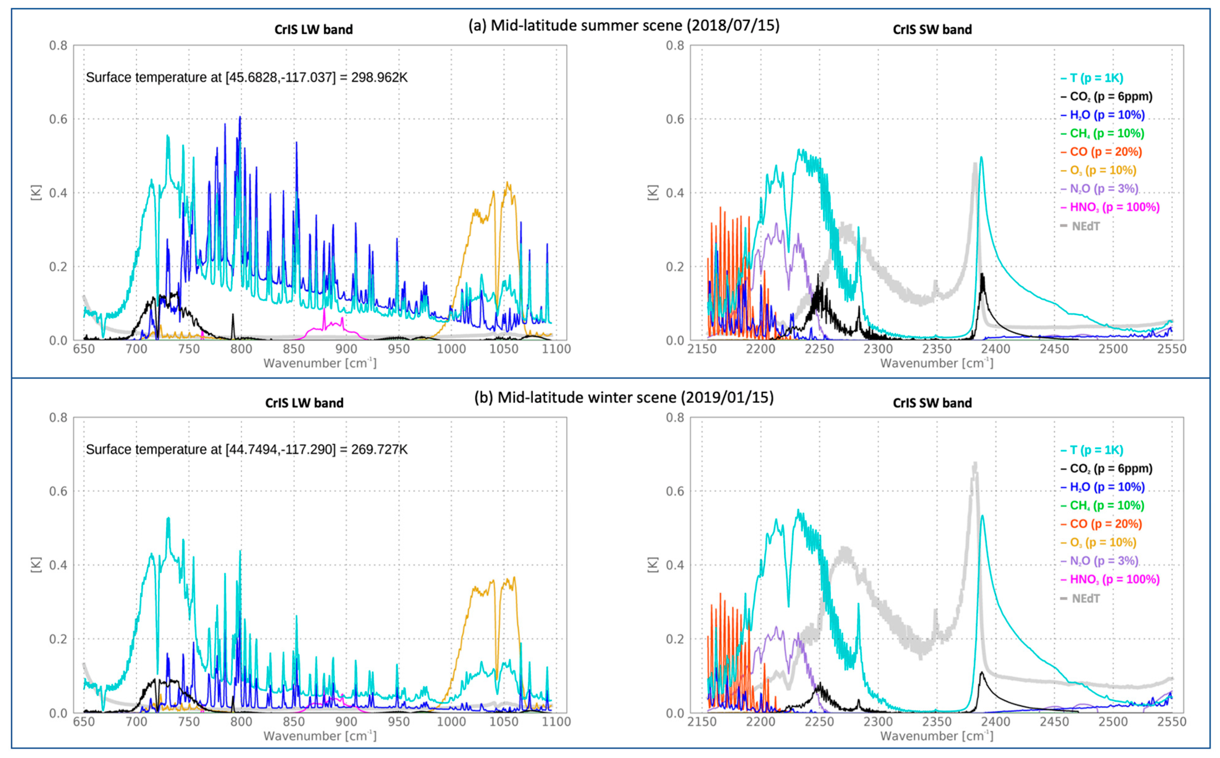
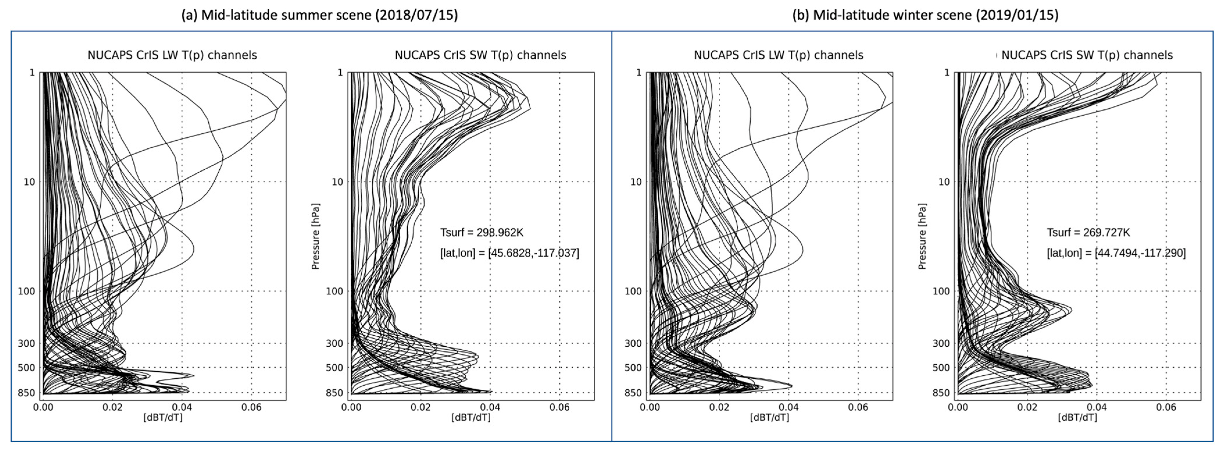
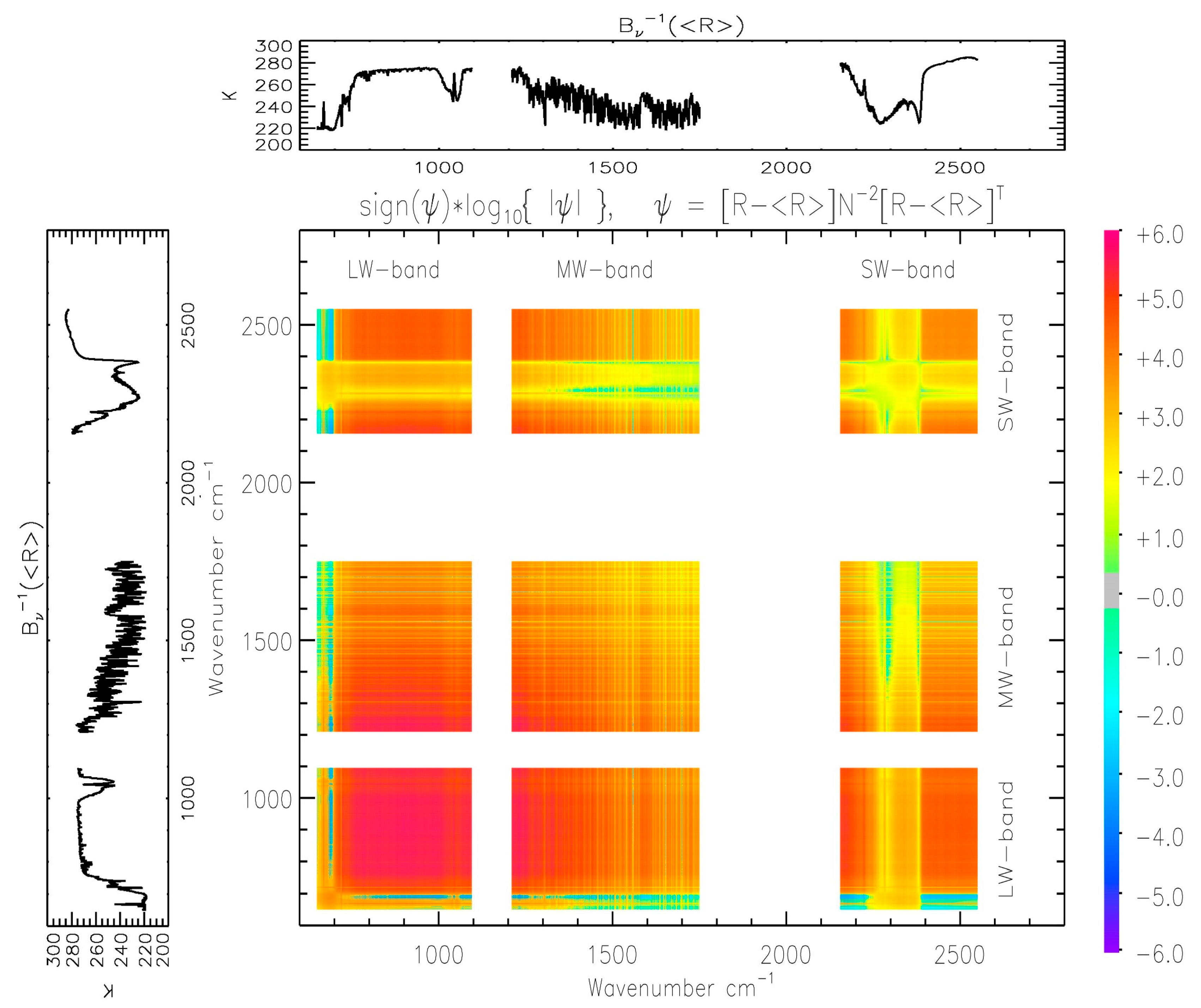
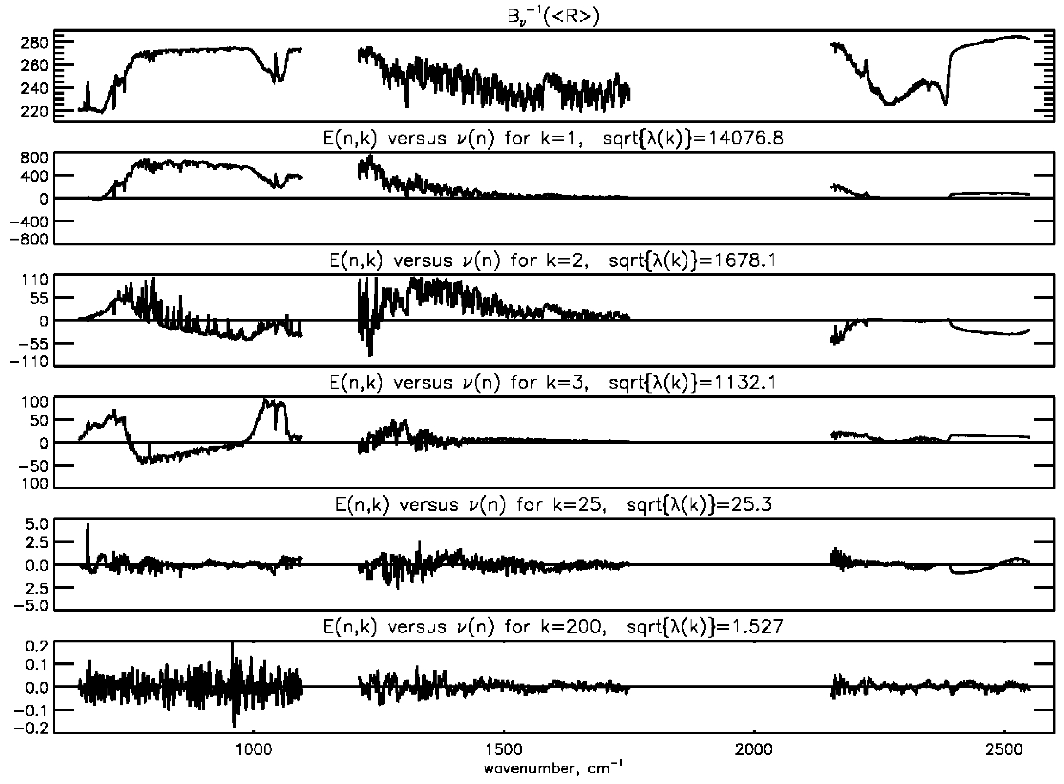
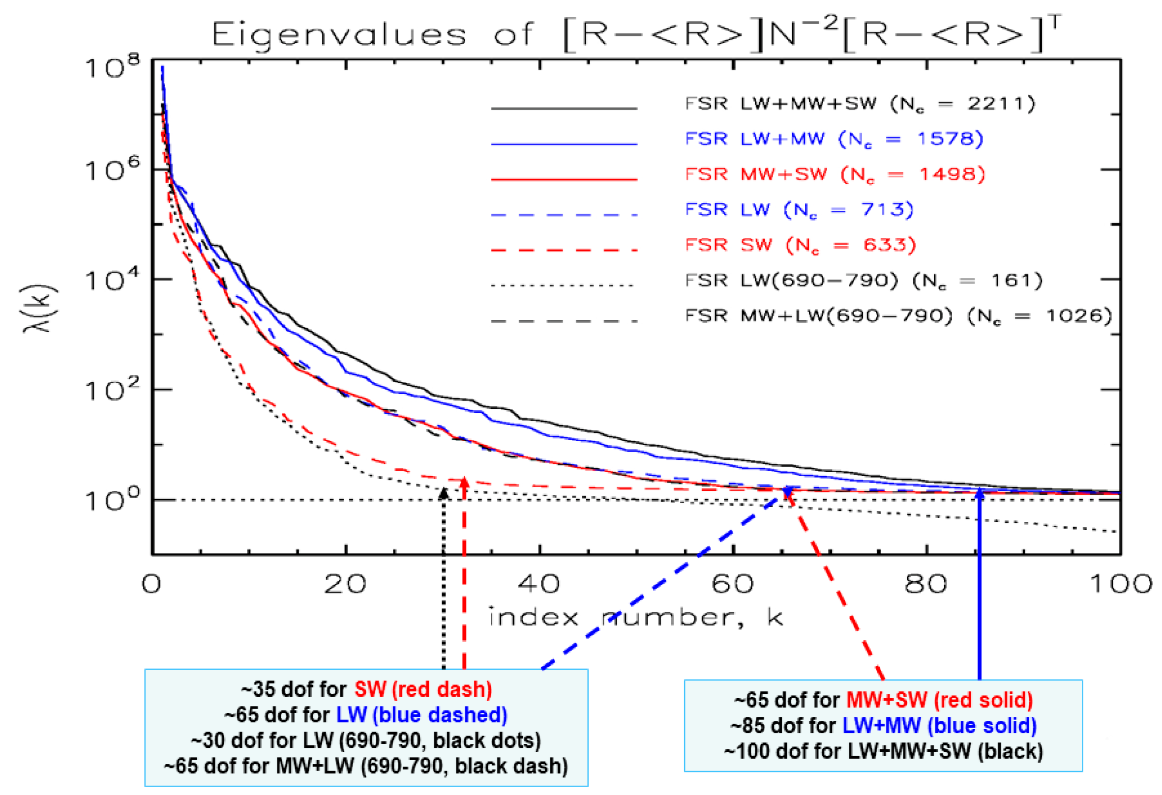
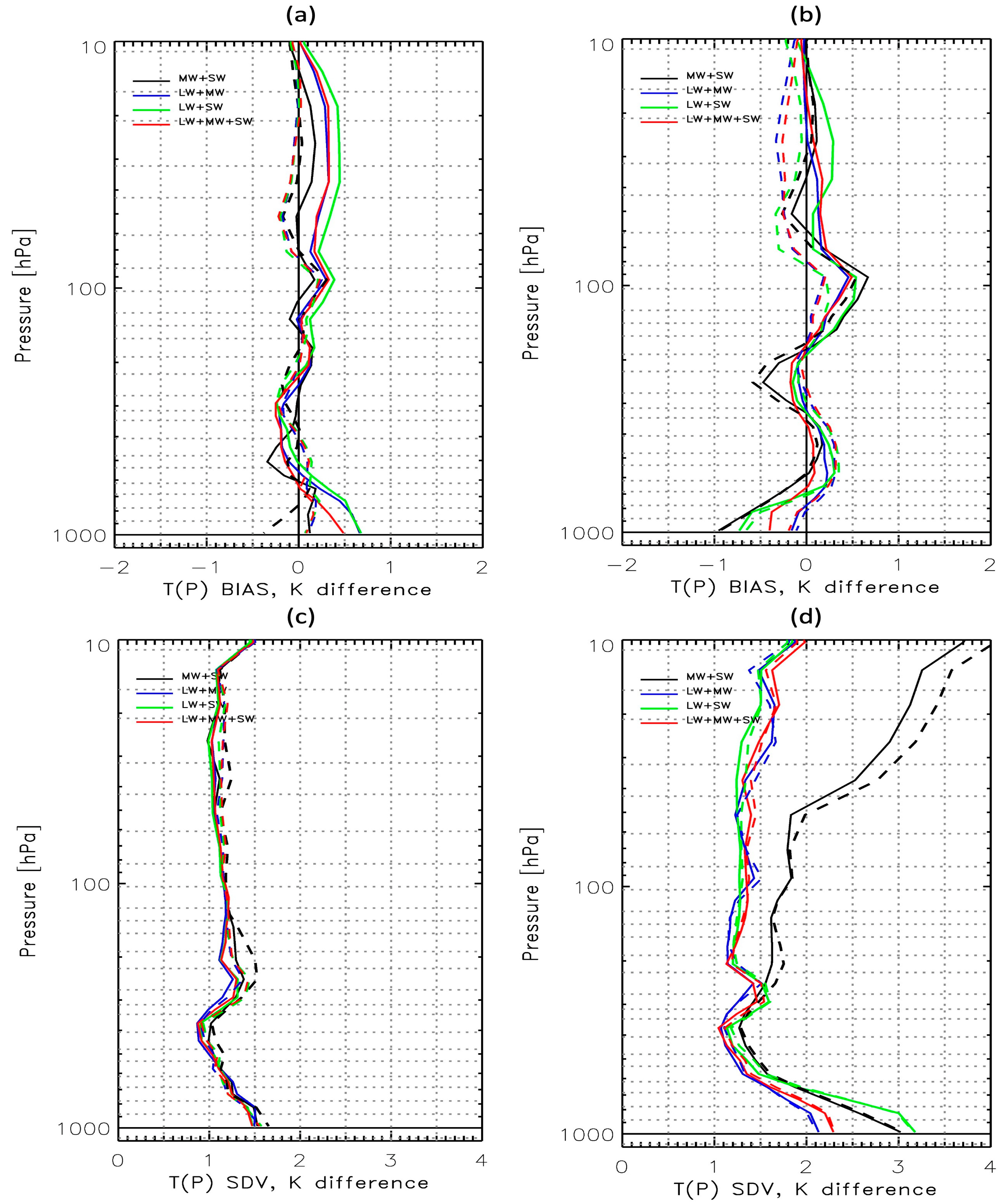
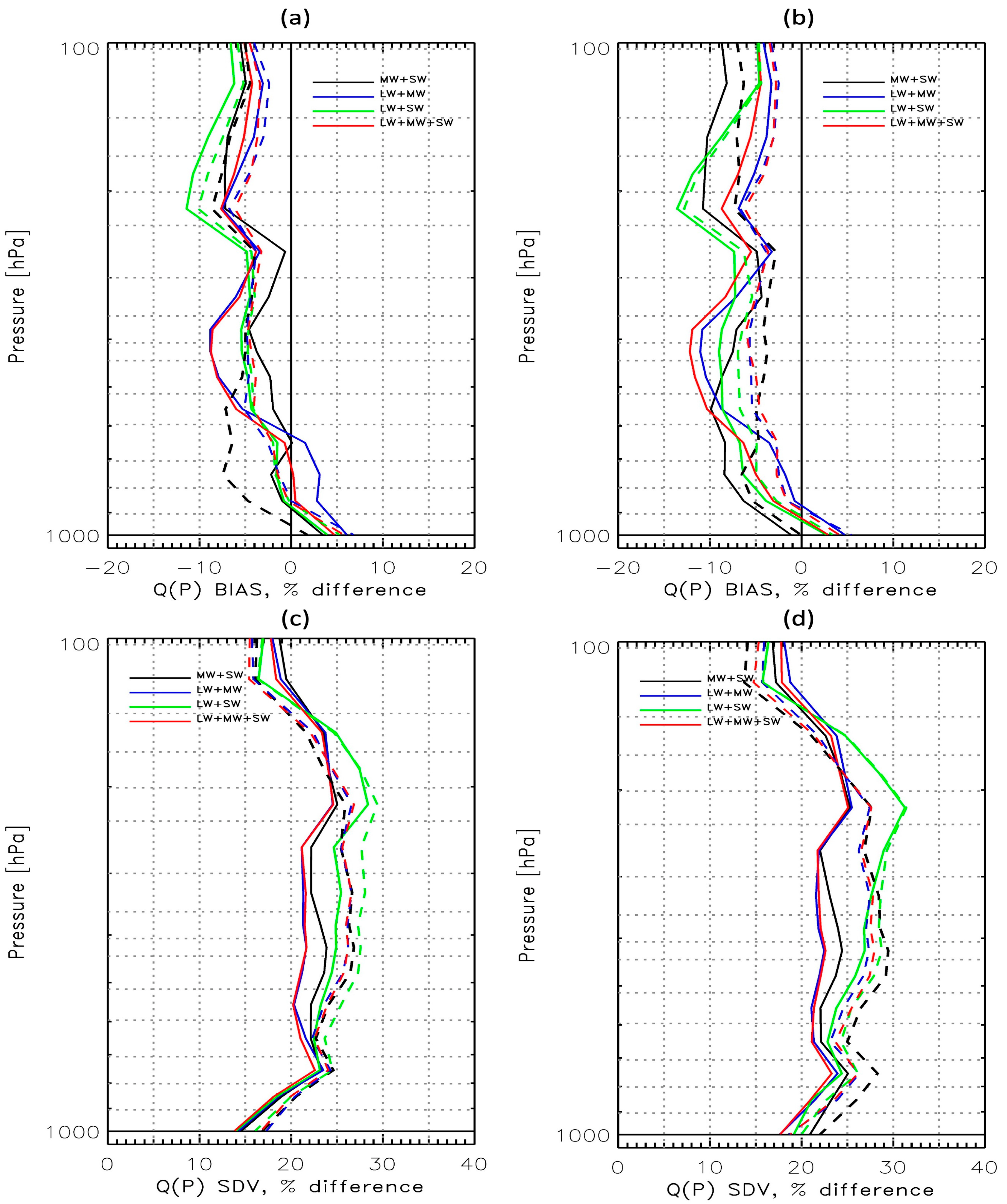
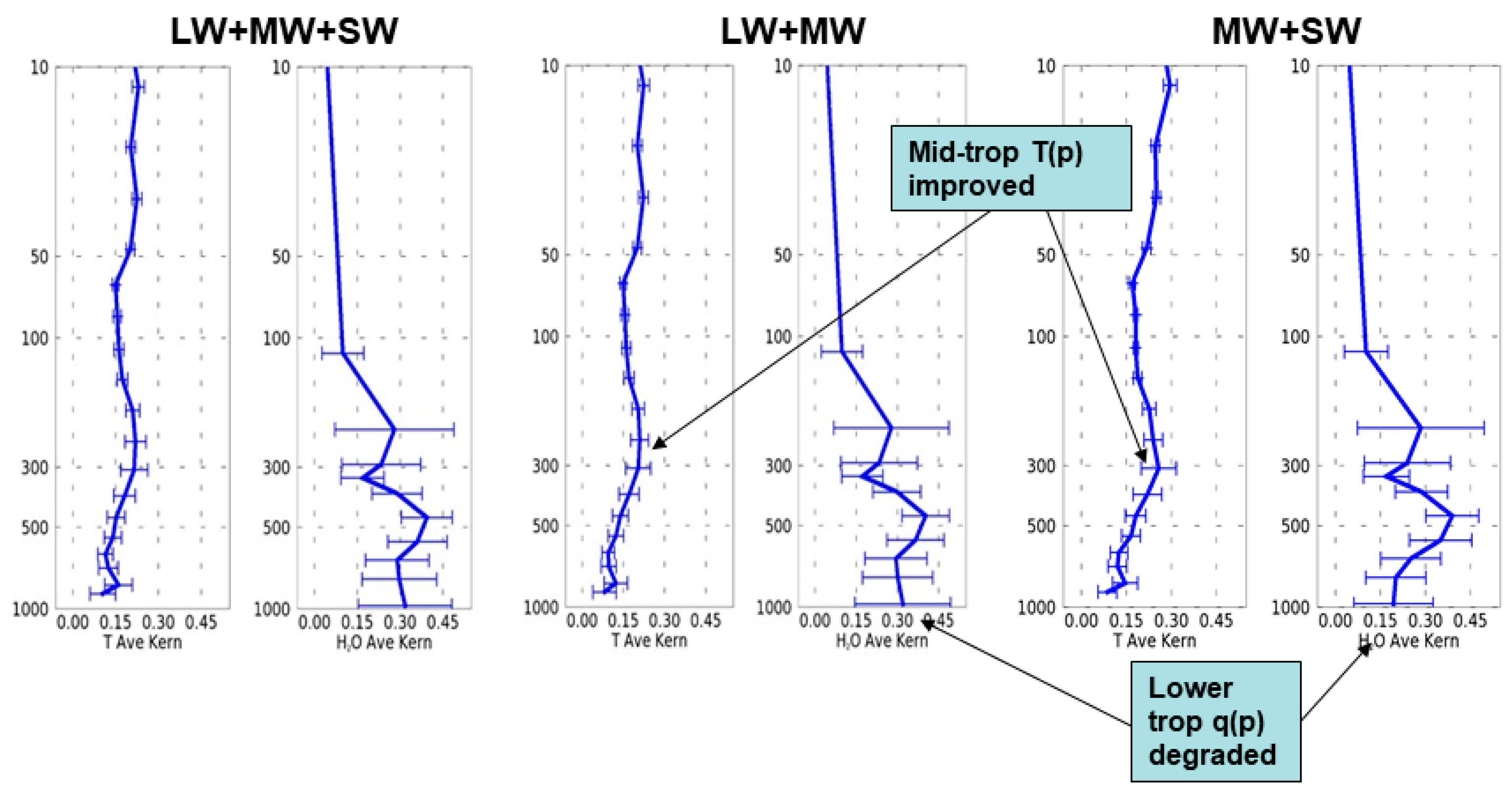
Table 1.
CrIS instrument noise as NEΔT and NEΔN for three different scene brightness temperatures (BT) in Kelvin [K]. For a constant NEΔN, the degree to which NEΔT varies with scene BT differs markedly between the CrIS longwave (LW; 650.0–1095 cm−1), midwave (MW; 1210–1750 cm−1) and shortwave (SW; 2155–2550 cm−1) bands.
| Scene BT | LW NEΔN | LW NEΔT | MW NEΔN | MW NEΔT | SW NEΔN | SW NEΔT |
|---|---|---|---|---|---|---|
| 200 K | 0.05 | 0.09 | 0.03 | 0.65 | 0.0046 | 9.7 |
| 250 K | 0.05 | 0.04 | 0.03 | 0.12 | 0.0046 | 0.5 |
| 300 K | 0.05 | 0.03 | 0.03 | 0.04 | 0.0046 | 0.07 |
Table 2.
A functional comparison between the CrIS longwave (LW) and shortwave (SW) infrared bands. This table is a summary of the work first published by [47].
Table 2.
A functional comparison between the CrIS longwave (LW) and shortwave (SW) infrared bands. This table is a summary of the work first published by [47].
| Variable | CrIS LW Band (~15 μm) | CrIS SW Band (4.3 μm) |
|---|---|---|
| Interfering gases in CO2 bands | H2O, O3, HNO3 | None |
| Vertical sounding range | 1 hPa to surface | 20 hPa to surface |
| Influence of solar radiation | Negligible | Must handle non-LTE and surface reflection |
| Planck function linearity | First order linearity | Highly nonlinear |
| Sensitivity of the Jacobian to scene temperature | Low | High |
| Tropospheric vertical resolution | 4 km | 2 km |
Table 3.
The total number of eigenvalues (λ) greater than or equal to unity indicates the number of independent pieces of information for an ensemble of measurements given by its covariance matrix. The number of λ ≥ 1 is also known as the degrees of freedom for signal (DOFS) and used as a metric for information content. This table summarizes the different CrIS channel configurations presented in Figure 5. Column 1 lists the channel combinations as being from the CrIS longwave (LW; 650.0–1095 cm−1), midwave (MW; 1210–1750 cm−1) and shortwave (SW; 2155–2550 cm−1). Column 2 lists the line type in Figure 5 that the tabled values correspond to, Column 3 is the total number of channels (Nc) in each subset configuration and Column 4 the DOFS.
| Channel Configuration | Line in Figure 5 | Nc | DOFS |
|---|---|---|---|
| LW + MW + SW | Solid black | 2211 | 100 |
| LW + MW | Solid blue | 1578 | 85 |
| MW + SW | Solid red | 1498 | 65 |
| LW-only | Dashed blue | 713 | 65 |
| MW-only | (not shown) | 865 | 60 |
| SW-only | Dashed red | 633 | 35 |
| LW (690–790 cm−1) | Dotted black | 161 | 30 |
| MW + LW (690–790 cm−1) | Dashed black | 1026 | 65 |
Disclaimer/Publisher’s Note: The statements, opinions and data contained in all publications are solely those of the individual author(s) and contributor(s) and not of MDPI and/or the editor(s). MDPI and/or the editor(s) disclaim responsibility for any injury to people or property resulting from any ideas, methods, instructions or products referred to in the content. |
© 2023 by the authors. Licensee MDPI, Basel, Switzerland. This article is an open access article distributed under the terms and conditions of the Creative Commons Attribution (CC BY) license (https://creativecommons.org/licenses/by/4.0/).
Share and Cite
MDPI and ACS Style
Barnet, C.D.; Smith, N.; Ide, K.; Garrett, K.; Jones, E. Evaluating the Value of CrIS Shortwave-Infrared Channels in Atmospheric-Sounding Retrievals. Remote Sens. 2023, 15, 547. https://doi.org/10.3390/rs15030547
AMA Style
Barnet CD, Smith N, Ide K, Garrett K, Jones E. Evaluating the Value of CrIS Shortwave-Infrared Channels in Atmospheric-Sounding Retrievals. Remote Sensing. 2023; 15(3):547. https://doi.org/10.3390/rs15030547
Chicago/Turabian StyleBarnet, Chris D., Nadia Smith, Kayo Ide, Kevin Garrett, and Erin Jones. 2023. "Evaluating the Value of CrIS Shortwave-Infrared Channels in Atmospheric-Sounding Retrievals" Remote Sensing 15, no. 3: 547. https://doi.org/10.3390/rs15030547
Note that from the first issue of 2016, this journal uses article numbers instead of page numbers. See further details here.