
Detecting Urban Floods with Small and Large Scale Analysis of ALOS-2/PALSAR-2 Data

1
School of Knowledge Science, Japan Advanced Institute of Science and Technology, Nomi 923-1292, Ishikawa, Japan
2
International Research Institute of Disaster Science, Tohoku University, Sendai 980-8572, Japan
*
Author to whom correspondence should be addressed.
Remote Sens. 2023, 15(2), 532; https://doi.org/10.3390/rs15020532
Submission received: 6 December 2022
/
Revised: 5 January 2023
/
Accepted: 7 January 2023
/
Published: 16 January 2023
(This article belongs to the Special Issue Toward an Application of Remote Sensing Technology for Decision Making during Natural Disasters)
Abstract
:When a large-scale flood disaster occurs, it is important to identify the flood areas in a short time in order to effectively support the affected areas afterwards. Synthetic Aperture Radar (SAR) is promising for flood detection. A number of change detection methods have been proposed to detect flooded areas with pre- and post-event SAR data. However, it remains difficult to detect flooded areas in built-up areas due to the complicated scattering of microwaves. To solve this issue, in this paper we propose the idea of analyzing the local changes in pre- and post-event SAR data as well as the larger-scale changes, which may improve accuracy for detecting floods in built-up areas. Therefore, we aimed at evaluating the effectiveness of multi-scale SAR analysis for flood detection in built-up areas using ALOS-2/PALSAR-2 data. First, several features were determined by calculating standard deviation images, difference images, and correlation coefficient images with several sizes of kernels. Then, segmentation on both small and large scales was applied to the correlation coefficient image and calculated explanatory variables with the features at each segment. Finally, machine learning models were tested for their flood detection performance in built-up areas by comparing a small-scale approach and multi-scale approach. Ten-fold cross-validation was used to validate the model, showing that highest accuracy was offered by the AdaBoost model, which improved the F1 Score from 0.89 in the small-scale analysis to 0.98 in the multi-scale analysis. The main contribution of this manuscript is that, from our results, it can be inferred that multi-scale analysis shows better performance in the quantitative detection of floods in built-up areas.
1. Introduction
Recently, the effects of climate change have increased in terms of extreme rainfall events [1]). Rapid urbanization has accelerated the impacts related to climate changes in many parts of the world [2]). In Japan, the 2018 floods caused severe damages in parts of western Japan from 28 June to 8 July 2018. When a large-scale flood disaster occurs, it is important to identify the flood areas in a short time in order to effectively support the affected area afterwards. For flood detection, Synthetic Aperture Radar (SAR) is promising. Many attempts have been made to detect flooded areas by utilizing the characteristics of backscattering coefficients in SAR data, which show lower values in flooded areas due to the principle of specular reflection. A number of methods that take advantage of this property have been reported in previous studies ([3,4,5,6,7,8,9,10]). For example, Moya et al. (2020) analyzed the possibility of applying training data acquired from the 2018 Japan floods to calibrate the discriminant function to detect flooded areas affected by the 2019 Hargis Typhoon using coherence calculated from SAR data [9,11,12]. Liang et al. (2020) developed a new approach to detect flooded areas by applying a global thresholding approach and local thresholding approach to Sentinel-1 SAR data [13].
However, it is difficult to detect flooded areas simply by detecting areas with lower backscattering coefficients in densely built-up areas. This is because backscattering coefficients in areas with building side walls show higher values in SAR imagery due to layover effects and double-bounce reflection. Therefore, even built-up areas that are flooded can show higher backscattering coefficient values. This characteristics leads to difficulties when detecting floods in built-up areas. Regarding this issue, previous studies have reported that complicated scattering in urban regions make it difficult to detect flooded areas ([10,14,15,16]). On the other hand, recent studies have reported successful examples of detecting flooded areas in built-up regions. For example, Liu et al. (2019) tried an approach to detect flooded areas based on the standard deviation of difference values of two time periods of coherence values [17]. Their paper reported that good performance could be shown in built-up areas. Li et al. (2019) developed a flood detection method for residential areas by combining coherence and intensity images and applying Bayes’ theorem, resulting in good accuracy [18]. In Liu et al. (2021), flood detection was conducted by dividing SAR images into fully flooded and partially flooded building areas; the authors reported that good performance in the detection of flooded areas could be confirmed even in built-up locations [19].
Other approaches have been reported as well. Efforts have been made to combine SAR-based approaches with other approaches, such as other sensors, simulations, and data. For example, Mason et al. (2021) attempted to improve the detection accuracy of flooded areas by integrating data from SAR-based analysis with hazard maps produced by numerical analysis [20]. This is one of the most successful examples for detecting urban floods, offering a detection accuracy of 94% on average and a false positive rate of only 9%. Tanguy et al. (2017) combined SAR data and hydraulic data, realizing improvements in flood detection [21]. Okada et al. (2021) integrated information from news reports with SAR image processing, resulting in improved accuracy [22].
As described above, a number of attempts have been made to detect flooded areas using SAR data under various conditions. Although several cases of accurate detection have been reported, further research is needed in order to generalize the method of detecting flooded areas in built-up areas.
In our study, we attempt to develop a method to detect floods in built-up areas with high accuracy and stability in order to investigate the effectiveness of multi-scale analysis of SAR data for detecting floods in built-up areas using only SAR data. The radar properties of flooded built-up areas are complicated, and it is sometimes difficult to classify pixels as flooded or not. In such cases, we formed the hypothesis that focusing on both the pixels of interest and the surrounding pixels could be a useful way to predict whether or not the pixels of interest represent flooding. For example, even if backscattering coefficients in areas of building side walls show higher values inside flooded areas, other areas that are near to the building side walls may show lower backscattering coefficient due to specular reflection. In this case, these surrounding changes can be good evidence to predict whether or not there is flooding in the area of interest. Several studies have reported multi-scale analysis for flood detection. Martinis et al. (2013) used a combination of MODIS satellite imagery and TerraSAR-X data to detect inundated areas [23]. Giordan et al. (2018) used various sensors with different spatial resolutions [24]. Xu et al. (2021) used a Convolutional Neural Network and multi-scale analysis to detect inundation; however, they reported that there are outstanding issues yet to be solved in the detection of flooding in dense built-up areas. Thus, it remains necessary to improve the detection of dense urban areas by multi-scale analysis [25]. However, the effectiveness of multi-scale analysis for detecting floods in built-up areas has not yet been evaluated quantitatively by integrating small-scale and large-scale analysis of SAR data. If we can quantitatively evaluate the effectiveness of multi-scale analysis in detecting flooding in built-up areas by conducting such a comparative analysis, we might be able to propose more stable and accurate flood assessment methods. Therefore, the following research question was set in this study: “How much does multi-scale analysis improve the accuracy of flood detection in built-up areas compared to small-scale analysis when using pre- and post-event SAR data?” To answer this question, we aimed to evaluate the effectiveness of multi-scale SAR analysis for flood detection in built-up areas using a comparative scale approach.
For the multi-scale based approach, we applied the region-growing method to divide the imagery into small-scale segments and large-scale segments. In this introduction, we summarize several types of segmentation method and explain the differences between the region-growing method and other segmentation approaches.
In order to perform multi-scale analysis, a segmentation process was applied to SAR images. In previous studies, a number of segmentation methods have been proposed. In this section, we briefly introduce “Superpixel segmentation methods”, “Watershed segmentation methods”, the “Active contour model”, and the “Region growing method”. The superpixel segmentation method divides an image into small regions with homogeneous color and texture characteristics. This method can reduce the noise in the image as well as the computational load. In recent years, several kinds of studies to extend these methods to multi-scale segmentation have been proposed; Lang et al. (2018) proposed a superpixel segmentation method for polarimetric SAR images based on the Generalized Mean Shift method, while Zhang et al. (2022) proposed a multiscale superpixel segmentation method based on a minimum spanning tree that offers a highly accurate hierarchical segmentation method [26,27]. The watershed segmentation methods performs region segmentation by setting the source of regions called markers as local minima in the image and then expanding the regions to adjacent pixels. While it has the advantage of easy maintenance of closure and continuity, it has the disadvantage of over-segmentation in the case of images in which a large number of local minima are obtained in the image. Marcin et al. (2017) applied the watershed segmentation method to SAR polarimetric images to detect river channels [28]. They reduced the computation time of the segmentation process by decreasing the computational complexity as much as possible. Ijitona et al. (2014) applied watershed segmentation to SAR images to detect ice floe size distribution [29]. The active contour model is a method of segmenting regions in which a closed surface is placed to enclose the object in the image from the inside or outside. The function of the surface is defined as an energy function, and the method estimates the surface with the minimum energy by repeatedly changing the position and shape of the surface to decrease its energy. In recent years, research has been conducted on the application of the level set method to PolSAR, which can solve the phase problem when dividing multiple objects in the active contour model. Braga et al. (2017) constructed a hierarchical level set method based on a median filter, which is a nonparametric curvature regularization filter, and used morphological operations for front propagation [30]. Jin et al. (2017) constructed a method for applying level set segmentation to high-resolution polarimetric SAR images and heterogeneous regions such as forests and vegetation areas based on a heterogeneous clutter model [31]. The region-growing method specifies a seed point in the image, examines the neighboring pixels of that pixel, and assigns the same label to pixels that satisfy predefined condition. In this study, the region-growing method was applied to divide images into small-scale segments, that isn superpixels, and large-scale segments; then, the spatial statistics in the large-scale segments were applied to the small-scale segments overlapping with those segments. A model was constructed to estimate the presence or absence of flooding for each small-scale segment. This study suggests that a multi-scale flood detection method can be very effective in detecting floods in built-up areas, which is one of the most difficult outstanding problems yet to be solved for SAR.
Table 1 summarizes the pros and cons of papers that are closely related to the present study. We were able to determine that there are a number of outstanding problems when using SAR imagery for flood detection in built-up areas. Although there have been an increasing number of reports showing good accuracy in the detection of floods in built-up areas using SAR, there remains considerable room for improvement. On the other hand, although theoretical studies on multi-scale analysis have been conducted in recent years (e.g., Zhang et al. (2022)), the application of the framework to flood detection in built-up areas has not yet been verified [26].
The novelty of this study is that we reveal the effectiveness of multi-scale analysis methods quantitatively for flood detection in built-up areas, which is been considered a difficult problem. For flood detection in built-up areas, difference images, correlation coefficient images, and pre- and post-event local standard deviation images were calculated, then the region-growing method applied at both small and large scales to estimate the attributes values of each segment. In our experiments, we applied three types of machine learning algorithms (decision tree, logistic regression and AdaBoost). We compared the results of the different models with a small-scale model and a model integrating both small and large scales using ten-fold cross-validation, and found that the F1 Score increased by 5% to 8.6% with multi-scale analysis compared to the case with only small-scale segments.
The remaining sections of this paper are organized as follows. Section 2 introduces the study area, the ALOS-2/PALSAR-2 images used in this study, and the validation data on flooded areas. In Section 3, we describe the method we developed for flood detection using multi-scale segmentation and machine learning models. In Section 4, we present and discuss our results. Finally, Section 5 provides our conclusions, summarizes our results, and suggests future research directions.
2. Study Area and Dataset
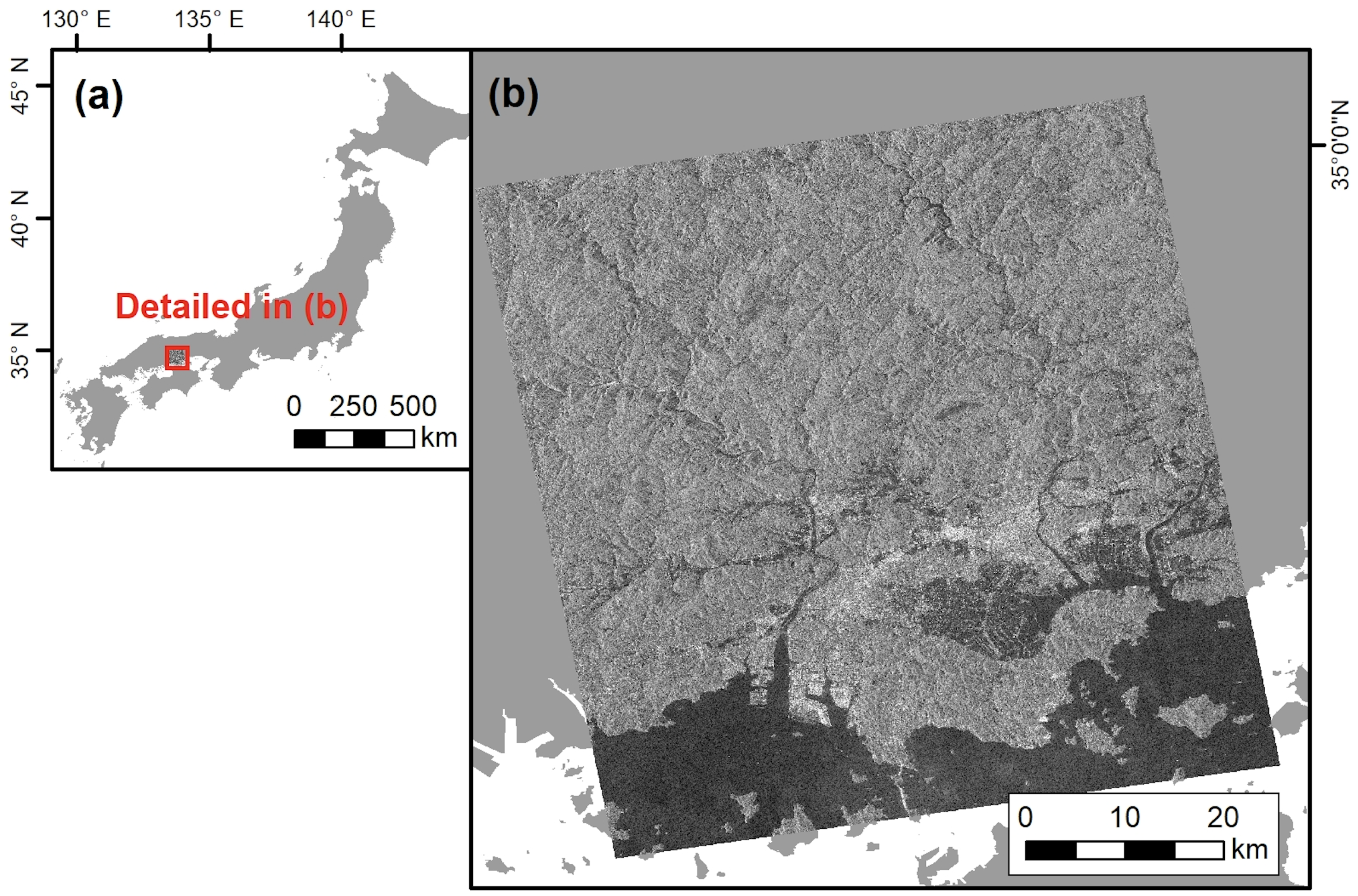
In this study, we used a set of ALOS-2/PALSAR-2 images taken before and after the disaster in Mabi-town, Okayama Prefecture, which was severely damaged by the July 2018 floods that occurred in Western Japan mainly from 28 June to 8 July 2018, as shown in Figure 1.
ALOS-2/PALSAR-2 is an L-band SAR launched in 2014. Several L-band SARs had been launched in Japan before, starting with JERS-1 in 1992, followed by ALOS/PALSAR in 2006. Its enhanced transmission power, expanded frequency bands, and dual-beam method with two independent beams for reception and chirp modulation, which can transmit multiple types of signals, enable ALOS/PALSAR to achieve higher resolution, a wider observation range, and higher visibility than conventional domestic L-band SARs [33].
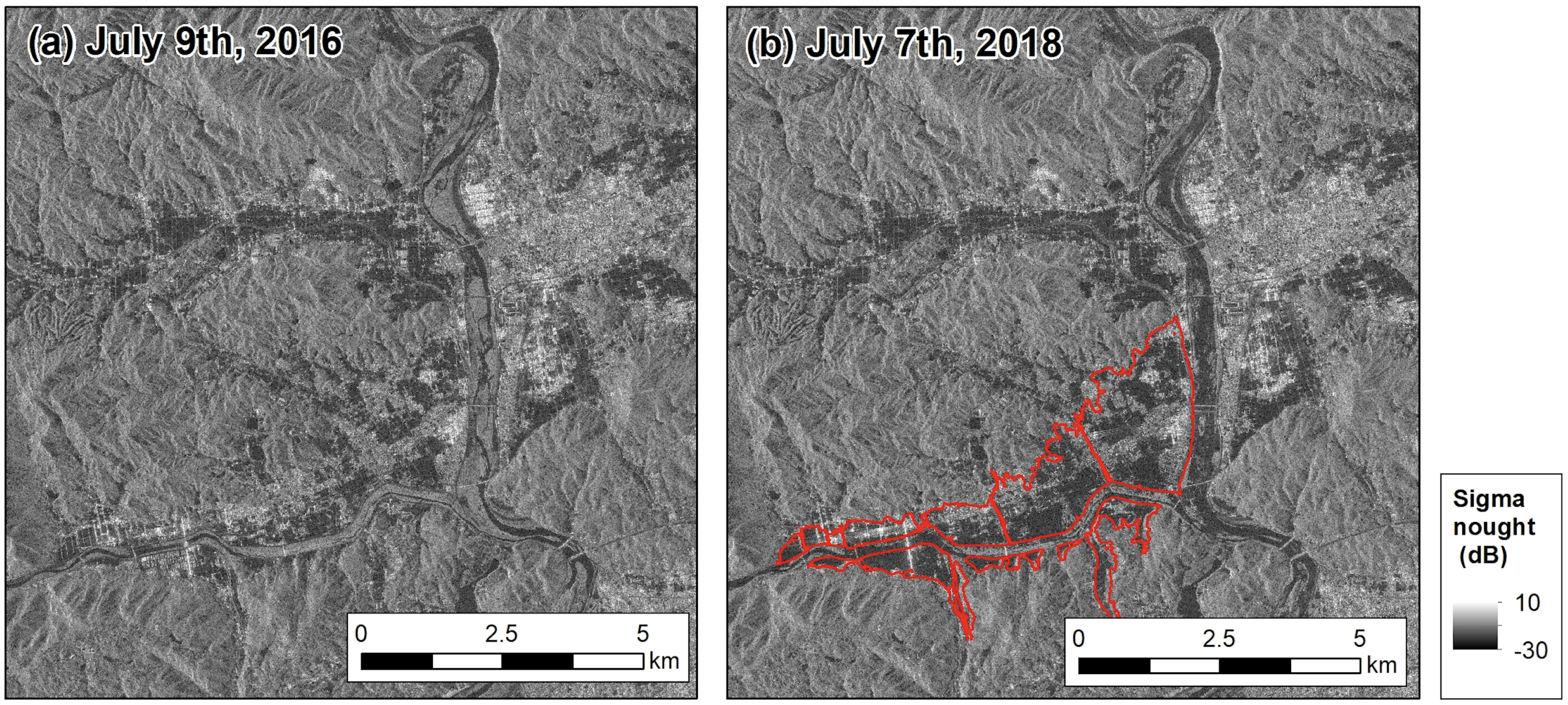
In this study, we used ALOS-2/PALSAR-2 imagery with a spatial resolution of 3 m observed in high-resolution mode (SM). The pixel spacing was 2.5 m, and the observation dates were 9 July 2016 and 7 July 2018. The images were taken in an ascending orbit at an angle of incidence of 38.7 degrees. Pre-event and post-event ALOS-2/PALSAR-2 imageries are shown in Figure 2.
3. Method
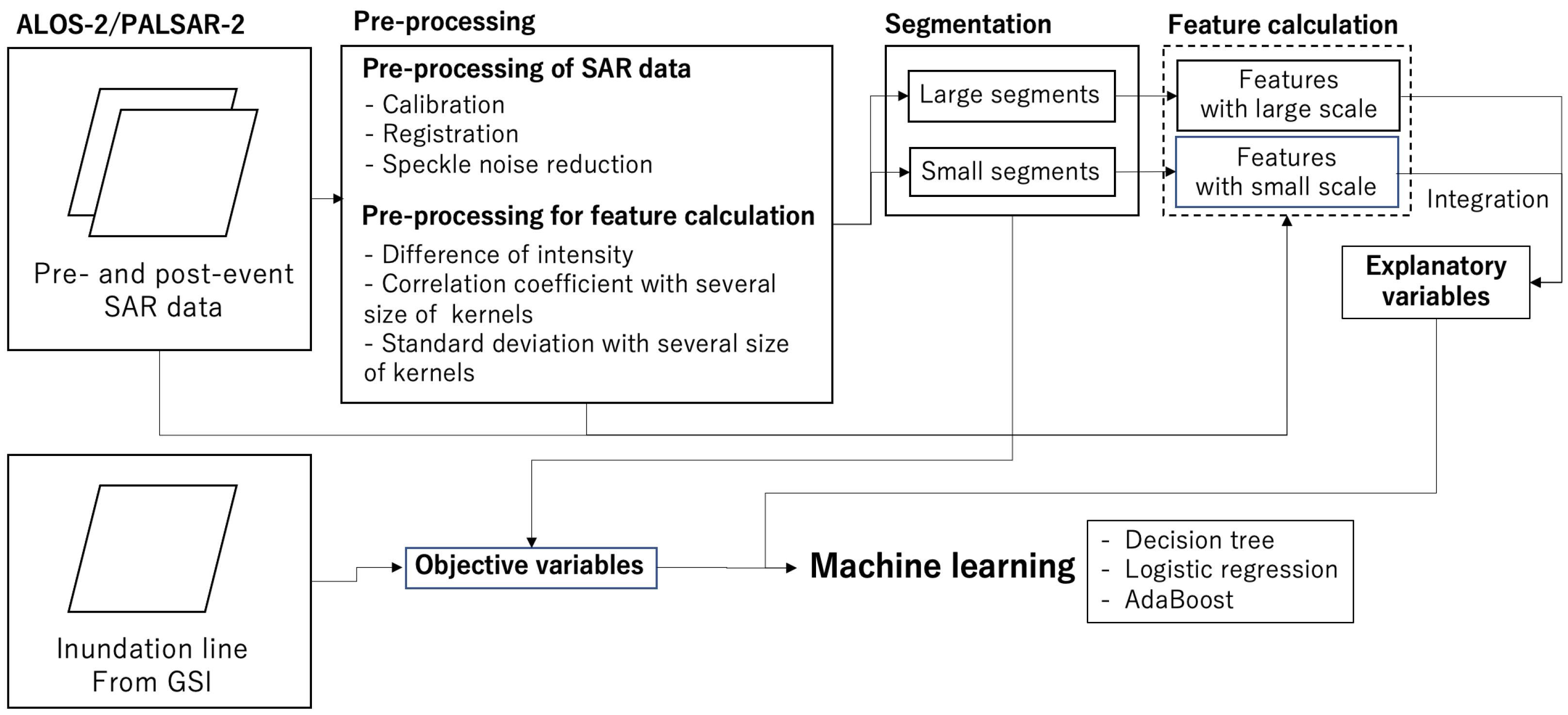
A general overview of this study is shown in Figure 3. First, pre-processing was applied to pre- and post-event ALOS-2/PALSAR-2 images that had been observed before and after the disaster, as shown in Section 3.1. As the ground truth data, data on the areas flooded in the 2018 Japan floods was downloaded from the website of Geospatial Authority of Japan and utilized, as detailed in Section 3.2. Next, feature calculation for creating the classifier was conducted, as described in Section 3.3. Pre-processing included calibration of the SAR imagery and feature detection by calculating the standard deviation of images and changes in the pre- and post-event sigma nought values. Then, a segmentation process was applied to obtain small-scale and large-scale segments, as described in Section 3.4. After that, features were calculated from the respective segments as explanatory variables, and “flood” or “not flood” information was applied to the data as objective variables, as described in in Section 3.5. Finally, three machine learning algorithms, namely, decision tree, logistic regression, and AdaBoost, were applied, and their performance was evaluated through the cross-validation. Based on the results, the performance of the small-scale and multi-scale approaches were compared, with the results of the comparison presented in Section 3.6.
3.1. Preprocessing of ALOS-2/PALSAR Data
First, Level 1.1 of ALOS-2/PALSAR-2 images before and after the disaster were prepared. For preprocessing of the ALOS-2/PALSAR-2 data, ENVI/SARscape software (Ver. 5.6) from Harris Geospatial solutions was used. First, a multi-look process was applied to the single-look complex data to produce an amplitude image. Multiple looks of range direction and azimuth direction were set as 1, and the grid size was set as 2.5 m. As the DEM for the multi-look process, SRTM was applied. After that, the amplitude images were converted to sigma nought images through geocoding and radiometric calibration. Next, the pre- and post-disaster images were registered based on their normalized cross-correlation. Finally, a Lee filter with a 3 * 3 pixel window was used for speck noise reduction. The backscattering coefficient images prepared in this way are shown in Figure 2.
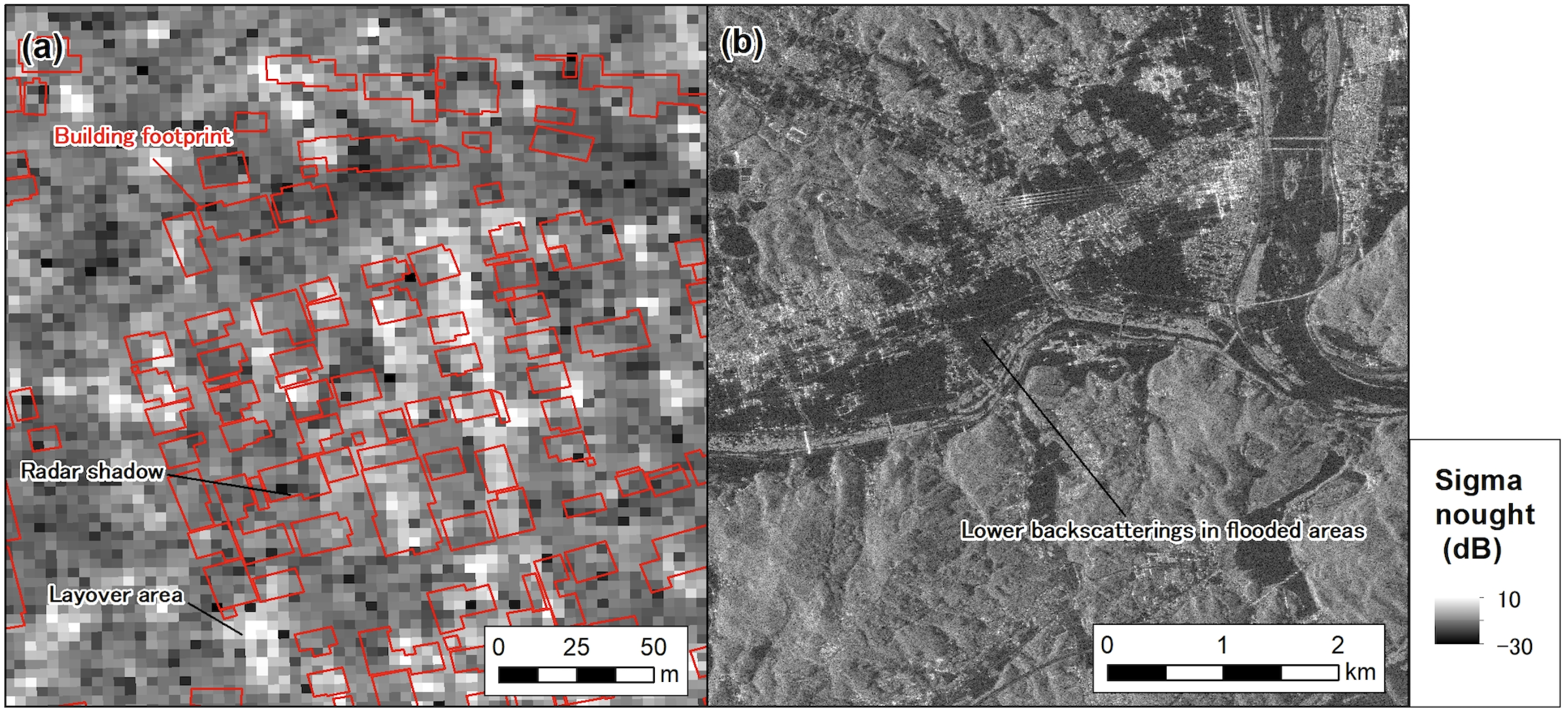
Zoomed images of built-up areas and flooded areas are shown in Figure 4. In Figure 4a, the building outlines are shown in red, and it can be seen that the bright backscattering areas with higher pixel values are concentrated on the locations of building outlines. It may be possible that these pixels were enhanced due to double-bounce reflections and layover effects on the walls facing the radar irradiation direction. On the other hand, other pixels show lower backscattering, which is caused by the radar shadow. In Figure 4b, lower backscattering can be observed in the area which was inundated by the floods. This is caused by the specular reflection. It is difficult to distinguish areas with radar shadows from those with specular reflection based solely on the value of the backscattering coefficient.
3.2. Preparation of Ground Truth Data
For verification, we referred to ground truth data from the Geospatial Information Authority of Japan (GSI). We used inundation area data interpreted by the GSI for Mabi-town, Kurashiki City, Okayama Prefecture, Japan. GSI uses aerial photos and video data taken on-site for the remote interpretation of flooded areas. Even though the reliability of the data on the extent of flooding is quite high, the data must be used carefully, as there is a possibility that certain areas that were inundated may not have been identified, and that areas that were not inundated may have been incorrectly indicated as inundated areas. The inundation line data are shown in Figure 2b.
3.3. Feature Calculation
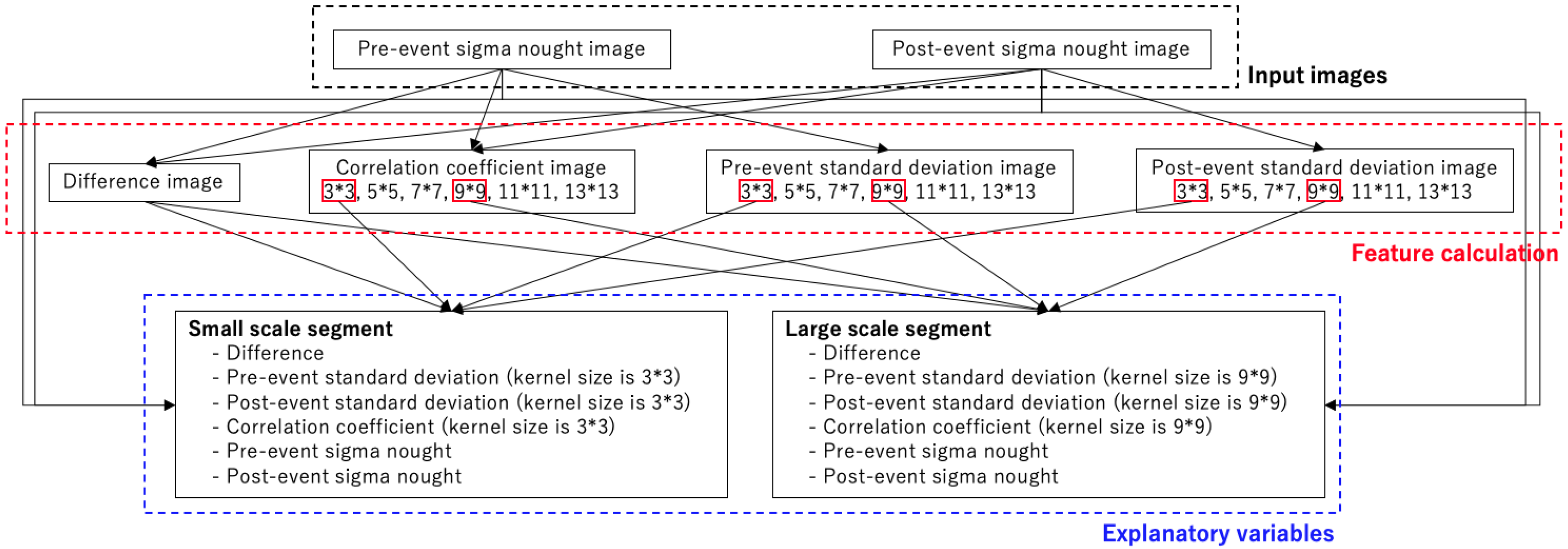
For feature calculation, change detection of pre- and post-event ALOS-2/PALSAR-2 images and texture images were calculated. For change detection, difference values of backscattering coefficients and correlation coefficients were calculated with several sizes of pixel windows. For calculating the texture image, local standard deviations on the pre- and post-event ALOS-2/PALSAR-2 images were calculated. The structure of this subsection is shown in Figure 5.
3.3.1. Differences in Pre- and Post-Event SAR Data
Differences were calculated using the following equation:
where and are the respective backscattering coefficients of the pre- and post-event SAR data.
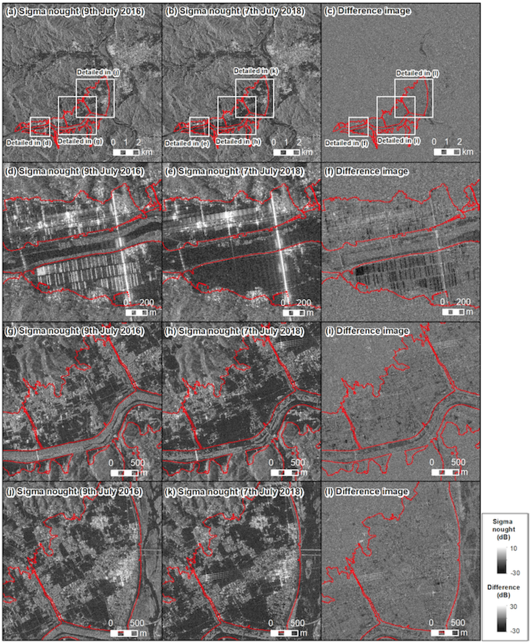
Examples of difference images are shown in Figure 6. Figure 6a is the pre-event sigma nought image, and Figure 6b is the post-event sigma nought image. Figure 6c is the difference image of Figure 6a,b. The other images from Figure 6d–i are zoomed images of them. As shown in Figure 6c, non-inundated areas are a gray color in most of the images, which means that the changes in the pixel values of the pre- and post-event sigma nought values were small. On the other hand, inside the inundation area certain areas in the difference images show a darker color or bright color. Zoomed images of the different regions are shown in Figure 6f,i,l. In Figure 6f, certain areas show a darker color in the lower part of image inside the inundation area. In these areas, uniformly-shaped structures were built pre-event. However, these disappeared in the post-event images; these areas were inundated by the floods. Therefore, the difference images show a darker color. In the upper part of Figure 6f, inside inundation area a darker color can be observed for the same reason. On the other hand, in Figure 6i,l it can be observed that a weak darker color is present in the whole inundation area. In order to extract those inundated areas where the pixel values themselves change little even though similar changes occur over a wide area, the segmentation process is considered more effective than simple thresholding.
The difference images show the location of pixels where changes in the backscattering coefficients occurred before and after the disaster, along with the degree of these changes. Furthermore, it is possible to infer what kind of change in the ground surface occurred by examining difference values calculated on the basis of whether the backscattering coefficient increased or decreased from before the disaster to after. For example, if the pixels of certain locations show higher backscattering in the pre-event image due to double-bounce reflections or layovers and show lower backscattering coefficients in the post-event images, it can be predicted that these pixels may be located in flooded areas. However, because these double reflections and layovers occur in the case of both structures and moving objects such as cars, it cannot be concluded that flooding has necessarily occurred at locations where the backscattering coefficient decreases from pre-event to post-event.
On the other hand, if objects are installed in the earth’s surface after the disaster in areas where no objects existed before the disaster, the backscattering coefficients may show higher values in the post-event image than in the pre-event image due to layover or double reflections. In addition, there might be cases in which layover areas are changed if objects are installed after the disaster.
Therefore, although various physical changes occurring on the ground surface can be predicted from the difference values, it is sometimes difficult to detect flooding in built-up areas simply by thresholding due to the complexity of scattering characteristics.
The degree of change in the difference value at a particular pixel depends on the value of the backscattering coefficient before the disaster, though the simple magnitude of the difference value does not necessarily represent the physical change in the ground surface. For example, in pixels where the backscattering coefficient is originally not strongly enhanced by layover, it can be expected that the backscatter coefficient will not decrease much even if the location is inundated. From the above, it can be understood that while the difference value is an effective indicator in determining the presence or absence of flooding, it is difficult to determine the presence or absence of flooding solely by using difference images.
3.3.2. Correlation Coefficients of Pre- and Post-Event SAR Data
The correlation coefficient image was estimated by calculating the correlation of pixels before and after the disaster in the pixel window based on the following formula:
where the and are the respective backscattering coefficients of pre- and post-event SAR data, is the variance, and is the covariance. The output values range from −1 to 1. Depending on the size of the area to be evaluated, the size of the pixel window needs to be changed. When examining the trend of the change of pixels before and after the disaster in a wide area, a wider pixel window should be used. On the other hand, when analyzing the changes in a local area, the size of the pixel window should be small.
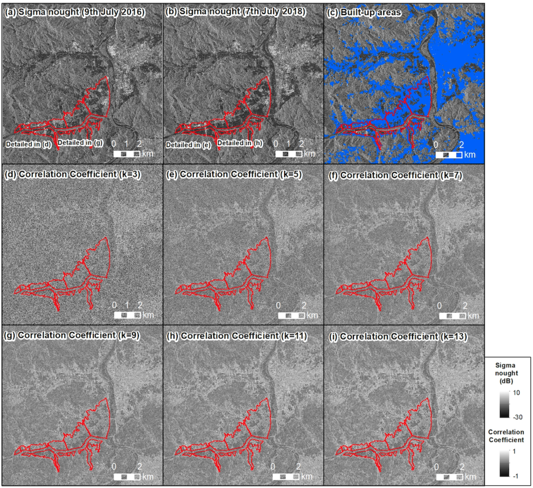
Correlation coefficient images were calculated as shown in Figure 7. Unlike the results of the difference value calculations, this correlation coefficient shows a certain similarity in the pre- and post-event SAR data.
In the correlation coefficient images, structures show higher values because the areas and backscattering coefficients of pre- and post-event sigma nought images do not change drastically without physical changes in the area. Depending on the size of the pixel window, the correlation coefficient values of built-up areas show different characteristics. As shown in Figure 7, built-up areas show higher color in area as a whole, and the boundary of built-up areas and other areas becomes clear. On the other hand, in built-up areas in the correlation coefficient image with the a kernel size of 3, the boundary of built-up areas and other areas are ambiguous, and even the built-up areas show relatively higher color. It can be inferred from this that the built-up areas with flooding have lower correlation coefficient values than those of non-flooded areas, as the radar properties of layover effects and radar shadow are changed. These changes contribute to detection of flooding in built-up areas.
3.3.3. Standard Deviation Images of Pre- and Post-Event SAR Data
We calculated the standard deviation values of each image taken before and after the disaster according to several sizes of kernels:
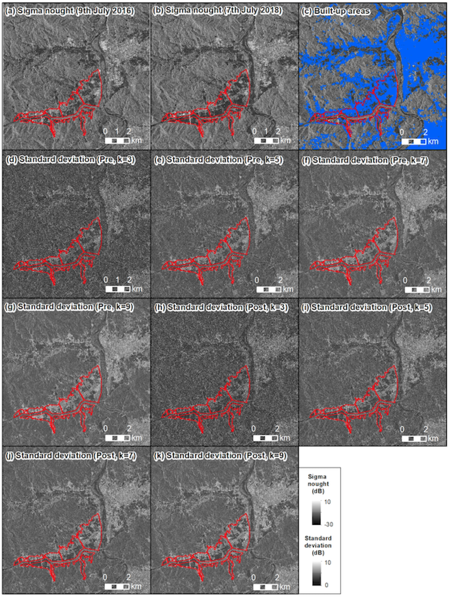
where is the standard deviation, is a pixel value inside the kernel, and is the average of pixel values inside the kernel. If the variance inside the kernel is high, then the standard deviation is higher. This is closely related to the spatial characteristics of the SAR images. The appropriate window size for capturing these spatial characteristics is considered to vary depending on the ground surface object of interest. If ground surface objects change significantly before and after the disaster, the values of these standard deviations can be expected to change significantly as well.
Standard deviation images were calculated as shown in Figure 8. Figure 8 shows that in the built-up areas those pixels with higher and lower backscattering are densely concentrated in a small area resulting, in higher standard deviation values. Comparing the distribution of built-up areas in Figure 8c and the other figures from (d)–(k), it can be seen that the boundaries between built-up areas and other areas become clearer as the kernel size becomes larger. On the other hand, in areas such as those inundated by water, the pixels uniformly show lower values, resulting in a lower standard deviations. In flooded areas inside built-up areas, the standard deviations values show different characteristics from unflooded built-up areas.
These result show that standard deviation changes drastically according to whether or not both the layover area and shadow area are included in the pixel window. For example, if the bright area caused by the layover area and darker area caused by radar shadow are included in the pixel window for the standard deviation, the resulting value of the standard deviation is higher. On the other hand, if only one of the shadow or layover areas is included in the pixel window, the standard deviation shows a lower value. Thus, the standard deviation can be considered a good indicator for understanding the flooding situation in built-up areas.
3.3.4. Feature Comparison
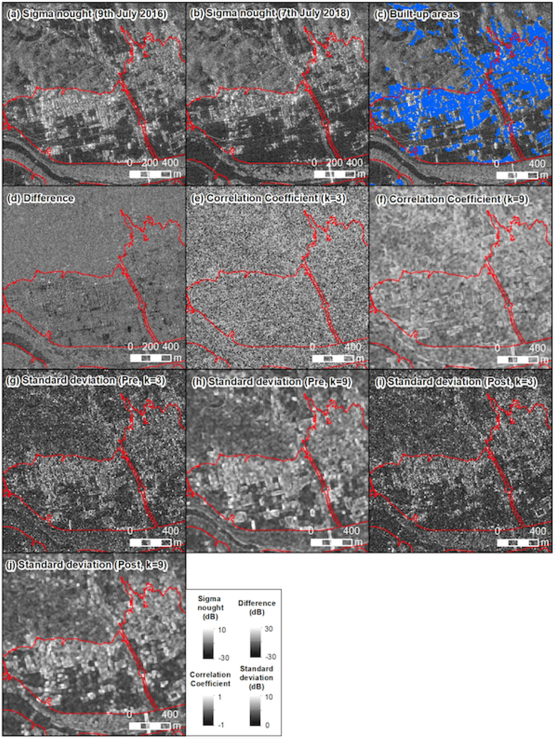
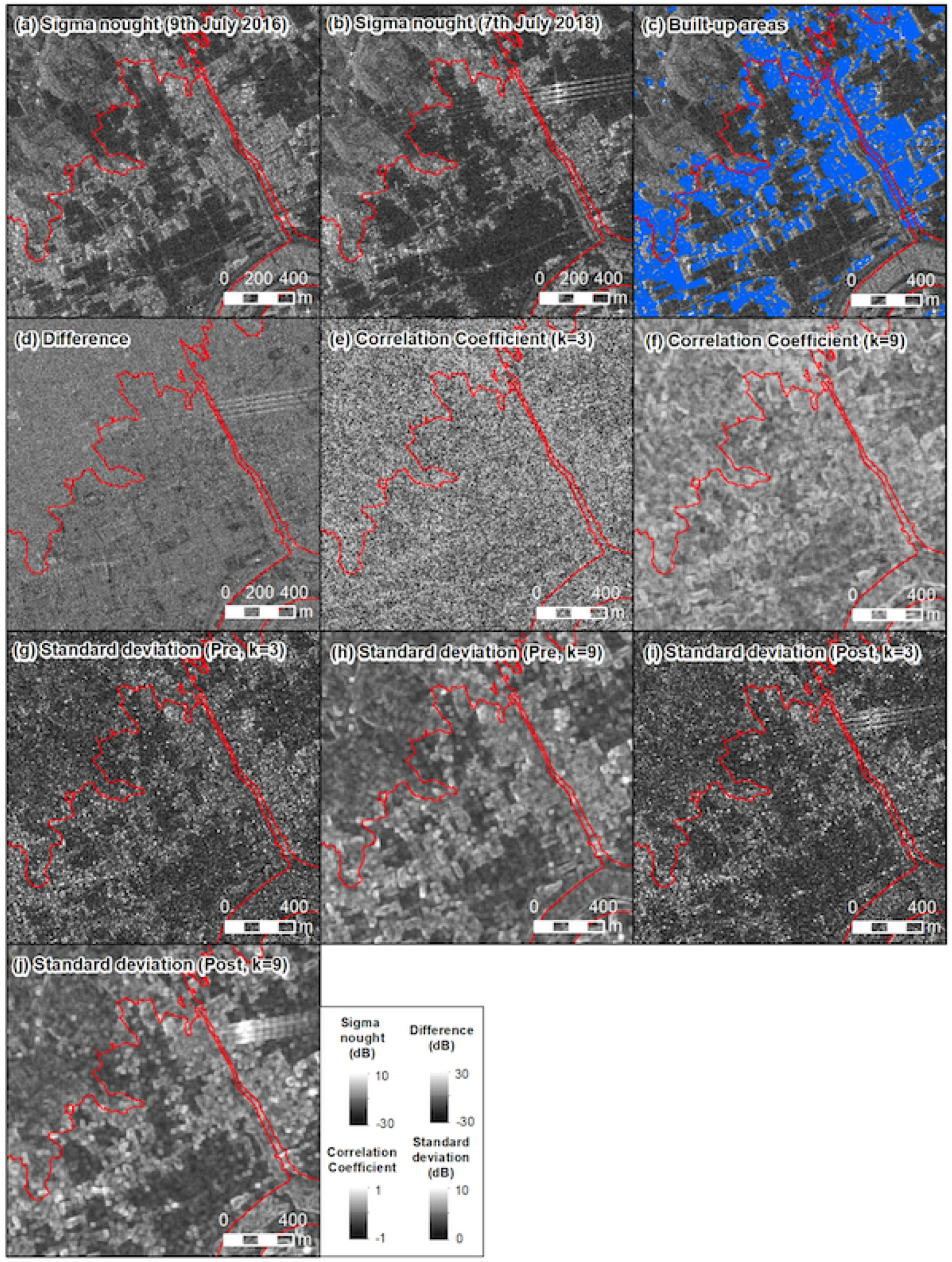
Detailed images of pre- and post-event sigma nought, difference, correlation coefficients and standard deviations are shown in Figure 9 and Figure 10. Different areas from flooded zones were selected and detailed imageries are shown in these figures. Figure 9 shows densely built-up areas. We can confirm that pre-event standard deviation images with a kernel size of 9 show higher values in built-up areas, as shown in Figure 9h. On the other hand, post-event standard deviation images with a kernel size of 9 show changes inside built-up areas, as shown in Figure 9h. From these differences, it can be inferred that standard deviation images might be a good indicator to detect changes in built-up areas caused by flooding. On the other hand, if we focus on Figure 9g,i, it can be seen that there are more localized changes in the standard deviation values. However, the confirmable changes are too sensitive, and the image appears to contains noise. Therefore, it might be considered that results with both smaller and larger kernel sizes should be utilized for flood detection. Regarding the difference image shown in Figure 9a, the flooded areas show relatively lower values. In addition, in the correlation coefficient images with the kernel size 3, as shown in Figure 9b, it is difficult to detect differences in built-up areas inside and outside the flooded area. However, in the correlation coefficient images with a kernel size of 9, as shown in Figure 9f, we can confirm that the correlation coefficient values of built-up areas show relatively lower values inside flooded areas than the outside of them. As can be seen in another zoomed image, shown in Figure 10, we can confirm the same characteristics as those in Figure 9.
3.4. Segmentation
Next, a segmentation process was carried out in order to perform a multi-scale analysis of the difference, correlation coefficient, standard deviation, and backscatter coefficient images. Segmentation was performed by applying the region-growing method using eCognition Developer 10.1 software from the Trimble Company [34].
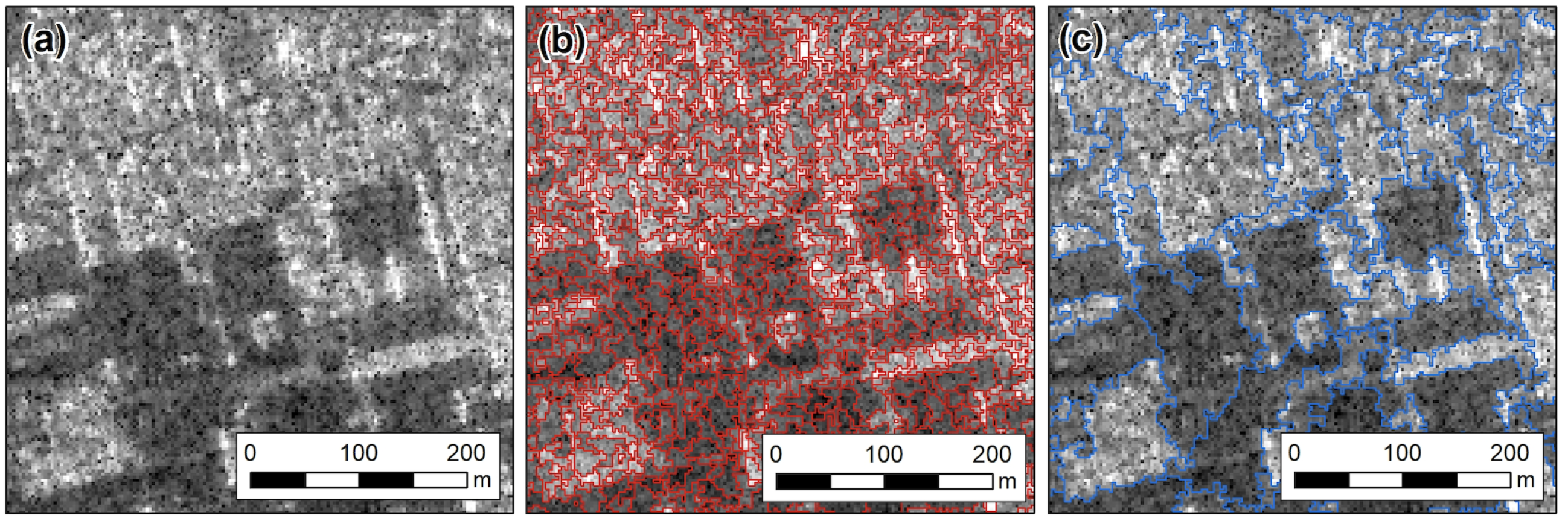
This region-growing method classifies images into homogeneous objects. In this study, the multi-resolution segmentation method was applied. First, the size of segments was decided. The setting of the appropriate segment size was carefully determined by examining the segment size and the characteristics of the surface objects, as shown in Figure 11.
To discuss the appropriate size of the objects, we first focused on the built-up areas. Built-up areas are characterized by the existence of bright areas from layover effects and darker areas from the radar shadow. Therefore, we considered that these bright and shadowed areas should be clearly discriminated by the segmentation process. Figure 11 shows an example of the segmentation process. Through trial and error, we tested several sizes of the scale parameter to classify the images into layover areas and shadowed areas. Finally, we classified the bright areas and darker areas inside the built-up areas when setting the scale parameter, through which we determined the small-scale segment size to be 5 (Figure 11b). On the other hand, we chose the size of the large-scale segment to ensure that the water areas and built-up areas could be distinguished. Through trial and error, we determined the scale parameter that could best classify the water areas shown by lower pixel values and built-up areas shown by higher pixel values to be 20, as shown in Figure 11c.
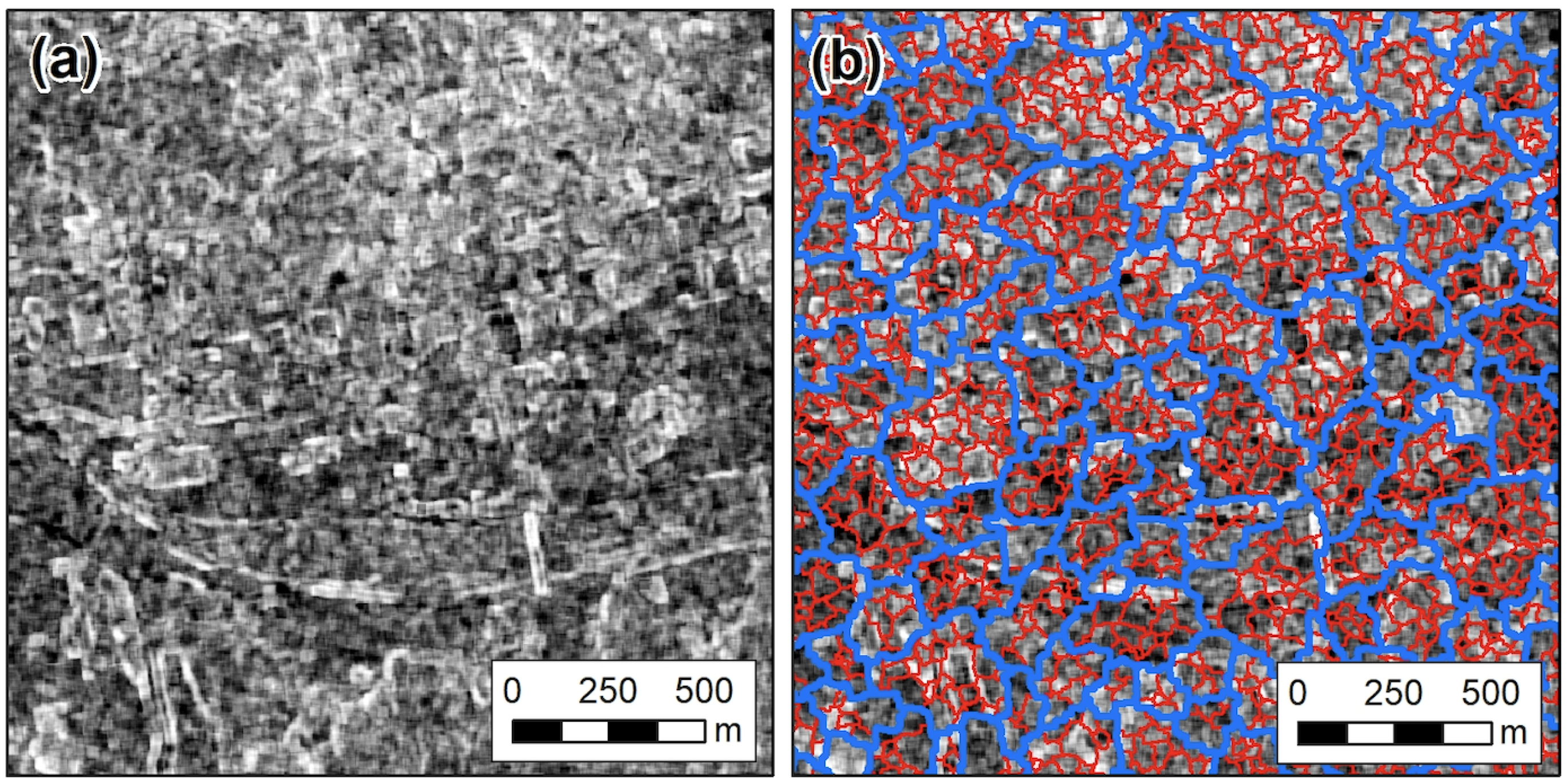
After determining the scale parameter of the large- and small-scale segments, we moved on to the multi-scale analysis. For the creation of large-scale and small-scale segments, the correlation coefficient images were utilized (Figure 12). We considered the correlation coefficient value to be suitable for creating the segments because it shows the similarity of pre- and post-event SAR data. Segments were created according to the degree of change in the pixels before and after the disaster; within each segment, the difference value, correlation coefficient, and standard deviation were calculated, and were used as the feature values for the machine learning performed in the latter part of this study.
We finalized the scale parameter for the small-scale segments as follows: scale parameter 5, shape 0.1, color 0.9, smoothness 0.5, and compactness 0.5; for the large-scale segments, the same values were a scale parameter of 20, shape 0.1, color 0.9, smoothness 0.5, and compactness 0.5.
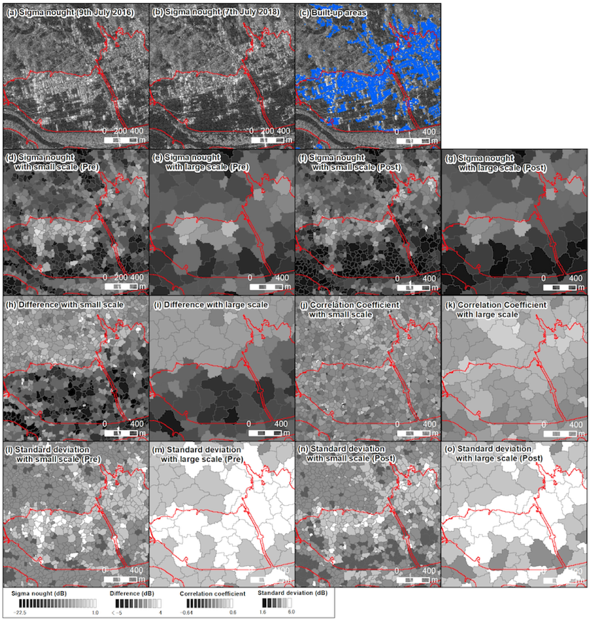
An example of the segmented results is shown in Figure 13. Compared with Figure 9, it can be seen that differences between the flooded and unflooded areas are clear. For example, Figure 9h shows lower values inside the flooded area than outside the flooded area, and the difference is more clear than in Figure 13d. By comparison with Figure 9h,i, it can be seen that Figure 9h shows more comprehensive differences; however, it does not show the more detailed changes visible in Figure 9i.
On the other hand, regarding of the correlation coefficient segments with the smaller scale, as shown in Figure 9j, it is difficult to see clear differences between the flooded and unflooded areas. However, as shown in Figure 9j, segments with built-up areas show higher correlation coefficient values in the large-scale segments.
In addition, small-scale and large-scale segments from standard deviation images show changes between the pre-event and post-event images, as shown in Figure 9i–o.
3.5. Calculation of Explanatory and Objective Variables Used in Machine Learning
The variables used in the calculation of explanatory and objective variables are listed in Table 2. For the detection of flooded in built-up areas, in this study we calculated a difference image, a pre-event standard deviation image, a post-event standard deviation image, correlation coefficient images before and after the disaster, a pre-event sigma nought image, and a post-event sigma nought image. After calculation of small and large scale segments from the correlation coefficient images, the respective mean values of these images were calculated at each segment. These values were used as explanatory variables for the machine learning model to detect flooded areas. In this part, we summarize how the kernel size of filters was selected for the small and large segments. First, the small-scale segment aims to detect local changes in the image before and after the disaster, especially in the layover and shadow regions in built-up areas. Therefore, for this purpose, a relatively smaller size of kernel size of 3 * 3 was selected as the filter size for calculating local standard deviations and correlation coefficients. In these data, the pixel spacing is 2.5 m, which means that the diameter of a single filter is 7.5 m. This is roughly the same size as the length of the layover area of common two-story Japanese houses, an incidence angle of 38.7 degrees. The height of a two-story building, which is a typical Japanese house, is 6 m. Therefore, if the incidence angle of observation is 38.7 degrees, the length of the layover area in the range direction is approximately 7.5 m. On the other hand, the kernel size of the larger area segment was decided to ensure that built-up areas and completely flooded areas could be distinguished. For this classification, a relatively larger perspective is needed. In this study, assuming a range length of the layover area of approximately 7.5 m, we set the kernel size to 9, which is large enough to include a range of layover areas. In this case, the diameter of one filter would be 22.5 m. However, in this study we did not conduct a sensitivity analysis to determine how the accuracy of detecting the flooded area changes when these filter sizes are changed. Therefore, in the future it remains necessary to determine the optimal filter size through sensitivity analysis.
The correlation coefficients and difference values of the pre- and post-event SAR data along with the backscattering coefficients and standard deviations of the pre- and post-event SAR data were utilized to calculate the mean values of these variables at each segment at both large and small scales. After that, by inputting the variables from the large segment to the spatially overlapping small segment, a corresponding set of explanatory variables were aggregated in the small segment.
For calculation of the objective variables, we used flood area maps published by the Geospatial Information Authority of Japan (GSI). Specifically, where the small segment and the inundation area map overlapped, the “flood” variable was assigned to the small segment and the “No flood” variable to the other segments.
Then, three types of machine learning model were tested. In this study, the decision tree, logistic regression, and AdaBoost algorithms were applied.
3.6. Validation of Machine Learning Models by Cross-Validation
Finally, to determine the effectiveness of the variables calculated by multi-scale analysis for detecting flooding in built-up areas, the model was evaluated in two cases: one in which only small segment values were calculated for flood detection, and one in which both the large and small segment values were incorporated into the analysis.
Cross-validation (n = 10) was used to evaluate the models. This study tested the validity of the above variables with the decision tree, logistic regression, and AdaBoost algorithms. Because the purpose of the study was to determine whether multi-scale analysis is effective in determining the inundation status of urban areas, making improvements to the machine learning models was outside of our scope. Therefore, the analysis here is limited to a simple comparison of the accuracy of inundation detection using features obtained from the multi-scale and small-scale approaches when using these simple machine learning models.
4. Results and Discussion
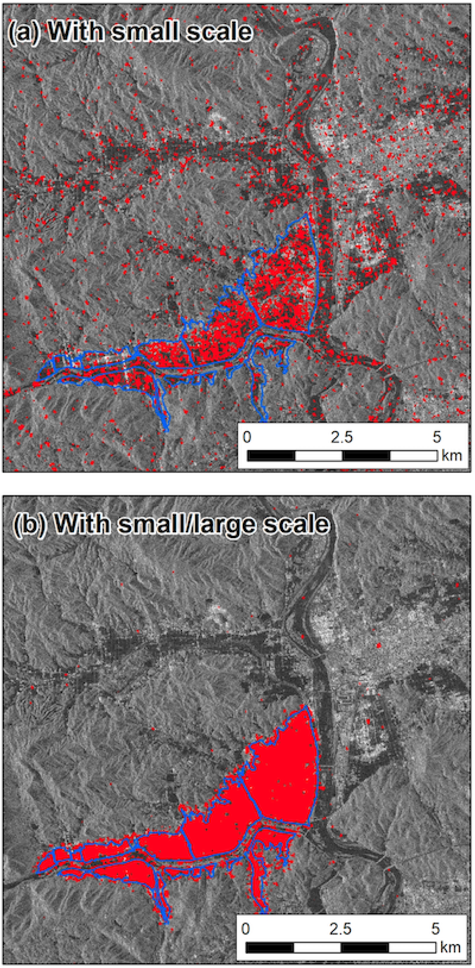
The cross-validation results of the small-scale and multi-scale analyses are shown in Table 3 and Table 4. For both models, the results show that multi-scale analysis is more effective. The inundation area detection results with the AdaBoost model, which enabled detection with particularly good accuracy, are shown in Figure 14 for the small-scale and multi-scale analyses. The blue lines in the figure show the boundary of the flooded area as published by the GSI, while the areas in red are the areas detected by the model proposed in this study; buildings are shown in white. Comparing these figures, it can be seen that both the small-scale and multi-scale analyses are able to identify the flooded areas in the built-up areas to an extent. However, in the small-scale analysis there are areas that are not detected well even within the actual flooded area; on the other hand, there are areas that are incorrectly determined to be flooded even though they are outside of the flooded area. From the results, we are able to confirm that multi-scale analysis greatly reduced such misclassifications, suggesting that accuracy can be improved by conducting an analysis that takes into account both local changes and changes in the surrounding area.
These results suggest that the multi-scale analysis approach proposed in this study is effective in understanding complicated flooded situations in built-up areas. In built-up areas, layovers and radar shadows are generally concentrated within a small area, making it difficult to identify inundation damage using SAR data. This study suggests that analysis based on various spatial scales may be effective in such locations.
5. Conclusions
In this study, we evaluated the effectiveness of multi-scale analysis of ALOS-2/PALSAR-2 data in understanding flood damage in built-up areas, using the flooded areas from the 2018 Japan floods as a case study. To perform a multi-scale analysis, machine learning models were created by segmenting pre- and post-flood event change detection images and correlation coefficient images, then using the features calculated from the pre- and post-disaster images as explanatory variables in large and small segments. Cross-validation was used to validate the model. Three types of models were tested: decision tree, logistic regression, and Adaboost. For all models, multi-scale analysis showed better performance than small-scale analysis alone. The highest accuracy was achieved with the AdaBoost model, which improved the F1 Score from 0.89 in the small-scale analysis to 0.98 in the multi-scale analysis. As our main findings, we can infer from the results that multi-scale analysis is effective for quantitative understanding of flood conditions in built-up areas. However, there are several limitations to this study. First, optimization of the filter size used during feature calculation was not addressed. This issue should be improved in future research through a sensitivity analysis. In addition, there is room for further generalization of the presented method. For example, if certain changes are made in terms of the physical characteristics used to describe built-up areas in the affected region and the observation angles of the SAR data, the proposed methods in this study are not applicable. Regarding the sophistication of the machine learning models, a sufficiently in-depth discussion could not be accomplished in this study. For future study, the different situations that may be present in various cases remains a concern to be addressed. New machine learning approaches could be developed to include adaptive functions in order to respond to such different situations.
Author Contributions
Conceptualization, H.G. and F.E.; methodology, H.G. and F.E.; software, H.G. and S.K.; validation, H.G.; formal analysis, H.G.; investigation, H.G.; resources, H.G. and F.E. and S.K.; data curation, H.G.; writing—original draft preparation, H.G.; visualization, H.G.; supervision, H.G. and S.K.; project administration, H.G. and S.K.; funding acquisition, H.G. and S.K. All authors have read and agreed to the published version of the manuscript.
Funding
This research was supported by a grant-in-aid from the Japanese Advanced Institute of Science and Technology (JAIST) and JSPS Grant-in-Aid for Scientific Research (20K15002, 21H05001).
Data Availability Statement
Not applicable.
Acknowledgments
This research was partly supported by Japan Advanced Institute of Science and Technology, Japan Aerospace Exploration Agency (JAXA), Tough Cyber-physical AI Research Center, Tohoku University, the Core Research Cluster of Disaster Science and the Co-creation Center for Disaster Resilience at Tohoku University. The satellite images were provided by Japan Aerospace Exploration Agency (JAXA) and preprocessed with ArcGIS and ENVI/SARscape 5.6, eCognition Developer ver.9 and the data analysis were implemented in Orange Data Mining software.
Conflicts of Interest
The authors declare no conflict of interest.
Abbreviations
The following abbreviations are used in this manuscript:
| SAR | Synthetic Aperture Radar |
| GSI | Geospatial Information Authority of Japan |
References
- Hettiarachchi, S.; Wasko, C.; Sharma, A. Increase in flood risk resulting from climate change in a developed urban watershed— The role of storm temporal patterns. Hydrol. Earth Syst. Sci. 2018, 22, 2041–2056. [Google Scholar] [CrossRef] [Green Version]
- Xing, Y.; Shao, D.; Liang, Q.; Chen, H.; Ma, X.; Ullah, I. Investigation of the drainage loss effects with a street view based drainage calculation method in hydrodynamic modelling of pluvial floods in urbanized area. J. Hydrol. 2022, 605, 127365. [Google Scholar] [CrossRef]
- Manjusree, P.; Prasanna, Kumar, L.; Bhatt, C.M.; Rao, G.S.; Bhanumurthy, V. Optimization of threshold ranges for rapid flood inundation mapping by evaluating backscatter profiles of high incidence angle SAR images. Int. J. Disaster Risk. Sci. 2012, 3, 113–122. [Google Scholar] [CrossRef] [Green Version]
- DeVriesa, B.; Huang, C.; Armston, J.; Huang, W.; Jones, J.W.; Lang, M.W. Rapid and robust monitoring of flood events using Sentinel-1 and Landsat data on the Google Earth Engine. Remote Sens. Environ. 2020, 240, 111664. [Google Scholar] [CrossRef]
- Huang, M.; Jin, S. Rapid flood mapping and evaluation with a supervised classifier and change detection in Shouguang using Sentinel-1 SAR and Sentinel-2 optical data. Remote Sens. 2020, 12, 2073. [Google Scholar] [CrossRef]
- Rahman, M.R.; Thakur, P.K. Detecting, mapping and analysing of flood water propagation using synthetic aperture radar (SAR) satellite data and GIS: A case study from the Kendrapara District of Orissa State of India. Egypt. J. Remote Sens. Space Sci. 2018, 21, S37–S41. [Google Scholar] [CrossRef]
- Matgen, P.; Hostache, R.; Schumann, G.; Pfister, L.; Hoffmann, L.; Savenije, H.H.G. Towards an automated SAR-based flood monitoring system: Lessons learned from two case studies. Phys. Chem. Earth 2011, 36, 241–252. [Google Scholar] [CrossRef]
- Wan, L.; Liu, M.; Wang, F.; Zhang, T.; You, H.J. Automatic extraction of flood inundation areas from SAR images: A case study of Jilin, China during the 2017 flood disaster. Int. J. Remote Sens. 2019, 40, 5050–5077. [Google Scholar] [CrossRef]
- Moya, L.; Mas, E.; Koshimura, S. Learning from the 2018 Western Japan heavy rains to detect floods during the 2019 Hagibis typhoon. Remote Sens. 2020, 12, 2244. [Google Scholar] [CrossRef]
- Giustarini, L.; Hostache, R.; Matgen, P.; Schumann, G.J.P.; Bates, P.D.; Mason, D.C. A change detection approach to flood mapping in urban areas using TerraSAR-X. IEEE Trans. Geosci. Remote Sens. 2012, 51, 2417–2430. [Google Scholar] [CrossRef]
- Moya, L.; Endo, Y.; Okada, G.; Koshimura, S.; Mas, E. Drawback in the Change Detection Approach: False Detection during the 2018 Western Japan Floods. Remote Sens. 2019, 11, 2320. [Google Scholar] [CrossRef] [Green Version]
- Moya, L.; Mas, E.; Koshimura, S. Sparse Representation-Based Inundation Depth Estimation Using SAR Data and Digital Elevation Model. IEEE J. Sel. Top. Appl. Earth Obs. Remote Sens. 2022, 15, 9062–9072. [Google Scholar] [CrossRef]
- Liang, J.; Liu, D. A local thresholding approach to flood water delineation using Sentinel-1 SAR imagery. ISPRS J. Photogramm. Remote Sens. 2020, 159, 53–62. [Google Scholar] [CrossRef]
- Schumann, G.J.P.; Neal, J.C.; Mason, D.C.; Bates, P.D. The accuracy of sequential aerial photography and SAR data for observing urban flood dynamics, a case study of the UK summer 2007 floods. Remote. Sens. Environ. 2011, 115, 2536–2546. [Google Scholar] [CrossRef]
- Pisut, N.; Fumio, Y.; Wen, L. Automated extraction of inundated areas from multi-temporal dual-polarization RADARSAT-2 images of the 2011 central Thailand flood. Remote Sens. 2017, 9, 78. [Google Scholar]
- Wen, L.; Fumio, Y. Detection of inundation areas due to the 2015 Kanto and Tohoku torrential rain in Japan based on multi-temporal ALOS-2 imagery. Nat. Hazards Earth Syst. Sci. 2018, 18, 1905–1918. [Google Scholar]
- Liu, W.; Yamazaki, F.; Maruyama, Y. Extraction of inundation areas due to the July 2018 Western Japan torrential rain event using multi-temporal ALOS-2 images. J. Disaster Res. 2019, 14, 445–455. [Google Scholar] [CrossRef]
- Li, Y.; Martinis, S.; Wiel, M.; Schlaffer, S.; Natsuaki, R. Urban flood mapping using SAR intensity and interferometric coherence via Bayesian network fusion. Remote Sens. 2019, 11, 2231. [Google Scholar] [CrossRef] [Green Version]
- Liu, W.; Fujii, K.; Maruyama, Y.; Yamazaki, F. Inundation assessment of the 2019 Typhoon Hagibis in Japan using multi-temporal Sentinel-1 intensity images. Remote Sens. 2021, 13, 639. [Google Scholar] [CrossRef]
- Mason, D.C.; Bevington, J.; Dance, S.L.; Revilla-Romero, B.; Smith, R.; Vetra-Carvalho, S.; Cloke, H.L. Improving urban flood mapping by merging Synthetic Aperture Radar-derived flood footprints with flood hazard maps. J. Abbr. 2021, 13, 1577. [Google Scholar] [CrossRef]
- Tanguy, M.; Chokmani, K.; Bernier, M.; Poulin, J.; Raymond, S. River flood mapping in urban areas combining Radarsat-2 data and flood return period data. Remote Sens. Environ. 2017, 198, 442–459. [Google Scholar] [CrossRef] [Green Version]
- Okada, G.; Moya, L.; Mas, E.; Koshimura, S. The potential role of news media to construct a machine learning based damage mapping framework. Remote Sens. 2021, 13, 1401. [Google Scholar] [CrossRef]
- Martinis, S.; Twele, A.; Strobl, C.; Kersten, J.; Stein, E. A multi-scale flood monitoring system based on fully automatic MODIS and TerraSAR-X processing chains. Remote Sens. 2013, 5, 5598–5619. [Google Scholar] [CrossRef] [Green Version]
- Giordan, D.; Notti, D.; Villa, A.; Zucca, F.; Calò, F.; Pepe, A.; Dutto, F.; Pari, P.; Baldo, M.; Allasia, P. Low cost, multiscale and multi-sensor application for flooded area mapping. Nat. Hazards Earth Syst. Sci. 2018, 18, 1493–1516. [Google Scholar] [CrossRef] [Green Version]
- Xu, C.; Zhang, S.; Zhao, B.; Liu, C.; Sui, H.; Yang, W.; Mei, L. SAR image water extraction using the attention U-net and multi-scale level set method: Flood monitoring in South China in 2020 as a test case. Geo-Spat. Inf. Sci. 2021, 25, 155–168. [Google Scholar] [CrossRef]
- Zhang, W.; Xiang, D.; Su, Y. Fast Multiscale Superpixel Segmentation for SAR Imagery. IEEE Geosci. Remote Sens. Lett. 2022, 19, 4001805. [Google Scholar] [CrossRef]
- Lang, F.; Yang, J.; Yan, S.; Qin, F. Superpixel Segmentation of Polarimetric Synthetic Aperture Radar (SAR) Images Based on Generalized Mean Shift. Remote Sens. 2018, 10, 1592. [Google Scholar] [CrossRef] [Green Version]
- Marcin, C. River channel segmentation in polarimetric SAR images: Watershed transform combined with average contrast maximisation. Expert Syst. Appl. 2017, 82, 196–215. [Google Scholar]
- Ijitona, T.B.; Ren, J.; Hwang, P.B. SAR Sea Ice Image Segmentation Using Watershed with Intensity-Based Region Merging. In Proceedings of the 2014 IEEE International Conference on Computer and Information Technology, Washington, DC, USA, 11–13 September 2014; pp. 168–172. [Google Scholar]
- Braga, A.M.; Marques, R.C.P.; Rodrigues, F.A.A.; Medeiros, F.N.S. A Median Regularized Level Set for Hierarchical Segmentation of SAR Images. IEEE Geosci. Remote Sens. Lett. 2017, 14, 1171–1175. [Google Scholar] [CrossRef]
- Jin, R.; Yin, J.; Zhou, W.; Yang, J. Level Set Segmentation Algorithm for High-Resolution Polarimetric SAR Images Based on a Heterogeneous Clutter Model. IEEE J. Sel. Top. Appl. Earth Obs. Remote Sens. 2017, 10, 4565–4579. [Google Scholar] [CrossRef]
- Cao, H.; Zhang, H.; Wang, C.; Zhang, B. Operational Flood Detection Using Sentinel-1 SAR Data over Large Areas. Water 2019, 11, 786. [Google Scholar] [CrossRef] [Green Version]
- JAXA, Advanced Land Observing Sattelite, ALOS-2 Project and PALSAR-2. Available online: https://www.eorc.jaxa.jp/ALOS-2/about/jpalsar2.htm (accessed on 30 May 2022).
- Benz, U.C.; Hofmann, P.; Willhauck, G.; Lingenfelder, I.; Heynen, M. Multi-resolution, object-oriented fuzzy analysis of remote sensing data for GIS-ready information. ISPRS J. Photogramm. Remote Sens. 2004, 58, 239–258. [Google Scholar] [CrossRef]
Figure 1.
Study area: (a) map of Japan, showing detail area; (b) ALOS-2/PALSAR-2 data capturing the study area.
Figure 1.
Study area: (a) map of Japan, showing detail area; (b) ALOS-2/PALSAR-2 data capturing the study area.

Figure 2.
ALOS–2/PALSAR–2 data: (a) Pre-event ALOS–2/PALSAR–2 data observed on 9 July 2016 and (b) post-event ALOS–2/PALSAR–2 data observed on 7 July 2018. The red line in (b) is the boundary of the flooded area as reported by the Geospatial Authority of Japan (GSI).
Figure 2.
ALOS–2/PALSAR–2 data: (a) Pre-event ALOS–2/PALSAR–2 data observed on 9 July 2016 and (b) post-event ALOS–2/PALSAR–2 data observed on 7 July 2018. The red line in (b) is the boundary of the flooded area as reported by the Geospatial Authority of Japan (GSI).

Figure 3.
General overview of the study.

Figure 4.
Zoomed image of ALOS-2/PALSAR-2 data: (a) built-up area and (b) flooded area.

Figure 5.
Structure of feature calculation. Red box indicates the kernel sizes that were selected to be used in the explanatory variables of machine learning models.
Figure 5.
Structure of feature calculation. Red box indicates the kernel sizes that were selected to be used in the explanatory variables of machine learning models.

Figure 6.
Examples of difference images: (a) sigma nought image on 9 July 2016; (b) sigma nought image on 7 July 2018; (c) difference image of (a,b); (d) zoomed image of (a); (e) zoomed image of (b); (f) difference image of (d,e); (g) zoomed image of (a); (h) zoomed image of (b); (i) difference image of (g,h); (j) zoomed image of (a); (k) zoomed image of (b); (l) zoomed image of (j,k).

Figure 7.
Examples of correlation coefficient images: (a) sigma nought image on 9 July 2016; (b) sigma nought image on 7 July 2018; (c) distribution of built-up areas, indicated by the blue color; (d–i) correlation coefficient image with (d) a kernel size of 3, (e) kernel size of 5, (f) kernel size of 7, (g) kernel size of 9, (h) kernel size of 11, and (i) kernel size of 13.

Figure 8.
Examples of standard deviation images: (a) sigma nought image on 9 July 2016; (b) sigma nought image on 7 July 2018; (c) distribution of built-up areas, illustrated by blue color; (d–g) are pre-event standard deviation images with (d) a kernel size of 3, (e) kernel size of 5, (f) kernel size of 7, and (g) kernel size of 9; (h–k) show the post-event standard deviation images with (h) a kernel size of 3, (i) kernel size of 5, (j) kernel size of 7, and (k) kernel size of 9.

Figure 9.
Examples of zoomed difference, correlation coefficient, and standard deviation images: (a) sigma nought image on 9 July 2016; (b) sigma nought image on 7 July 2018; (c) distribution of built-up areas; (d) difference image; (e) correlation coefficient image with kernel size 3; (f) correlation coefficient image with kernel size 9; (g) pre-event standard deviation image with kernel size 3; (h) pre-event standard deviation image with kernel size 9; (i) post-event standard deviation image with kernel size 3; (j) post-event standard deviation image with kernel size 9.

Figure 10.
More examples of zoomed difference, correlation coefficient, and standard deviation images: (a) sigma nought image on 9 July 2016; (b) sigma nought image on 7 July 2018; (c) distribution of built-up areas; (d) difference image; (e) correlation coefficient image with kernel size 3; (f) correlation coefficient image with kernel size 9; (g) pre-event standard deviation image with kernel size 3; (h) pre-event standard deviation image with kernel size 9; (i) post-event standard deviation image with kernel size 3; (j) post-event standard deviation image with kernel size 9.

Figure 11.
An example of segmentation with the smaller and larger scales: (a) pre-event SAR data; (b) small-scale segments; (c) large-scale segments.
Figure 11.
An example of segmentation with the smaller and larger scales: (a) pre-event SAR data; (b) small-scale segments; (c) large-scale segments.

Figure 12.
An example of segmentation in a correlation coefficient image: (a) correlation coefficient image and (b) segments with smaller and larger scales.
Figure 12.
An example of segmentation in a correlation coefficient image: (a) correlation coefficient image and (b) segments with smaller and larger scales.

Figure 13.
Examples of segmentation: (a) sigma nought image on 9 July 2016; (b) sigma nought image on 7 July 2018; (c) distribution of built-up areas; (d–o) segmentations with several types of variables: (d) pre-event sigma nought with small scale, (e) pre-event sigma nought with large scale, (f) post-event sigma nought with small scale, (g) post-event sigma nought with large scale, (h) difference image with small scale, (i) difference image with large scale, (j) correlation coefficient image with small scale, (k) correlation coefficient image with large scale, (l) pre-event standard deviation with small scale, (m) pre-event standard deviation with large scale, (n) post-event standard deviation with small scale, (o) post-event standard deviation with large scale.

Figure 14.
Results of flood detection with (a) small-scale approach and (b) integrated approach using both small and large scales.
Figure 14.
Results of flood detection with (a) small-scale approach and (b) integrated approach using both small and large scales.


Table 1.
Pros and Cons of existing methods.
| Author | Pros and Cons in Existing Approaches |
|---|---|
| Liu et al. (2019) | The authors conducted a combined analysis of coherence and intensity images to detect flooding in built-up areas. They reported that the extraction of flood features in built-up areas and rice fields showed good accuracy, with an F1 score of 0.78. Although this accuracy is good, there is room for improvement [17]. |
| Li et al. (2019) | The results showed that combining coherence and intensity images using a Bayesian network was effective for detecting flooded areas. Good accuracy was reported for built-up areas, with F1 Scores of 0.70–0.79. Although the accuracy was good, there remains room for improvement [18]. |
| Mason et al. (2021) | A flood foresight model was constructed based on flood hazard maps and SAR data. In the manuscript, 94% classification accuracy was offered based on the thresholding-based approach using only SAR data. However, the effectiveness of a multi-scale approach for detecting urban floods was outside the scope of this research [20]. |
| Giordan et al. (2018) | Using free and low-cost data and sensors, a multi-scale multi-sensor analysis was applied for flood detection. However, the authors reported that the accuracy decreased in built-up areas [24]. |
| Xu et al. (2021) | Flooded areas were detected with the attention U-net and multi-scale level set method. However, quantitative accuracy was not reported [25]. |
| Zhang et al. (2022) | A theoretical framework for multiscale analysis using X-band and Ku-band radar was proposed. However, its effectiveness in detecting floods in built-up areas was not evaluated [26]. |
| Cao et al. (2019) | An automatic thresholding approach was applied with the region-growing method to detect flooded areas. The paper reported 99.05% classification accuracy; however, performance with respect to detecting floods of built-up areas was not evaluated [32]. |
Table 2.
Explanatory variables calculated from smaller and larger segments.
| Variables Calculated from Small Segments | Variables Calculated from Large Segments |
|---|---|
| Difference values at small scale | Difference values at large scale |
| Pre-event standard deviation (k = 3) at small scale | Pre-event standard deviation (k = 9) at large scale |
| Post-event standard deviation (k = 3) at small scale | Post-event standard deviation (k = 9) at large scale |
| Correlation coefficient (k = 3) at small scale | Correlation coefficient (k = 9) at large scale |
| Pre-backscattering coefficient at small scale | Pre-backscattering coefficient at large scale |
| Post-backscattering coefficient at small scale | Post-backscattering coefficient at large scale |
Table 3.
Results of cross-validation with small-scale model.
| Model | Precision | Recall | F1 |
|---|---|---|---|
| Tree | 0.908 | 0.924 | 0.912 |
| Logistic regression | 0.889 | 0.918 | 0.892 |
| AdaBoost | 0.894 | 0.891 | 0.892 |
Table 4.
Results of cross-validation with small- and large-scale models.
| Model | Precision | Recall | F1 |
|---|---|---|---|
| Tree | 0.968 | 0.969 | 0.967 |
| Logistic regression | 0.942 | 0.947 | 0.942 |
| AdaBoost | 0.978 | 0.978 | 0.978 |
Disclaimer/Publisher’s Note: The statements, opinions and data contained in all publications are solely those of the individual author(s) and contributor(s) and not of MDPI and/or the editor(s). MDPI and/or the editor(s) disclaim responsibility for any injury to people or property resulting from any ideas, methods, instructions or products referred to in the content. |
© 2023 by the authors. Licensee MDPI, Basel, Switzerland. This article is an open access article distributed under the terms and conditions of the Creative Commons Attribution (CC BY) license (https://creativecommons.org/licenses/by/4.0/).
Share and Cite
MDPI and ACS Style
Gokon, H.; Endo, F.; Koshimura, S. Detecting Urban Floods with Small and Large Scale Analysis of ALOS-2/PALSAR-2 Data. Remote Sens. 2023, 15, 532. https://doi.org/10.3390/rs15020532
AMA Style
Gokon H, Endo F, Koshimura S. Detecting Urban Floods with Small and Large Scale Analysis of ALOS-2/PALSAR-2 Data. Remote Sensing. 2023; 15(2):532. https://doi.org/10.3390/rs15020532
Chicago/Turabian StyleGokon, Hideomi, Fuyuki Endo, and Shunichi Koshimura. 2023. "Detecting Urban Floods with Small and Large Scale Analysis of ALOS-2/PALSAR-2 Data" Remote Sensing 15, no. 2: 532. https://doi.org/10.3390/rs15020532
Note that from the first issue of 2016, this journal uses article numbers instead of page numbers. See further details here.