
MD3: Model-Driven Deep Remotely Sensed Image Denoising
by
 , , , ,
Zhenghua Huang
1,2 ,
,
Zifan Zhu
2,
Yaozong Zhang
2,
Zhicheng Wang
2 ,
,
Biyun Xu
2,
Jun Liu
3,
Shaoyi Li
4 and
Hao Fang
5,* 1
Artificial Intelligence School, Wuchang University of Technology, Wuhan 430223, China
2
School of Electrical and Information Engineering, Wuhan Institute of Technology, Wuhan 430205, China
3
State Key Laboratory of Information Engineering in Surveying, Mapping and Remote Sensing, Wuhan University, Wuhan 430079, China
4
College of Astronautics, Northwestern Polytechnical University (NWPU), Xi’an 710072, China
5
School of Electronic and Information Engineering, Wuhan Donghu University, Wuhan 430212, China
*
Author to whom correspondence should be addressed.
Remote Sens. 2023, 15(2), 445; https://doi.org/10.3390/rs15020445
Submission received: 30 November 2022
/
Revised: 31 December 2022
/
Accepted: 2 January 2023
/
Published: 11 January 2023
(This article belongs to the Special Issue Reinforcement Learning Algorithm in Remote Sensing)
Abstract
:Remotely sensed images degraded by additive white Gaussian noise (AWGN) have low-level vision, resulting in a poor analysis of their contents. To reduce AWGN, two types of denoising strategies, sparse-coding-model-based and deep-neural-network-based (DNN), are commonly utilized, which have their respective merits and drawbacks. For example, the former pursue enjoyable performance with a high computational burden, while the latter have powerful capacity in completing a specified task efficiently, but this limits their application range. To combine their merits for improving performance efficiently, this paper proposes a model-driven deep denoising (MD) scheme. To solve the MD model, we first decomposed it into several subproblems by the alternating direction method of multipliers (ADMM). Then, the denoising subproblems are replaced by different learnable denoisers, which are plugged into the unfolded MD model to efficiently produce a stable solution. Both quantitative and qualitative results validate that the proposed MD approach is effective and efficient, while it has a more powerful ability in generating enjoyable denoising performance and preserving rich textures than other advanced methods.
1. Introduction
Remote sensing imaging technology, based on the theory of electromagnetic waves, is an approach to produce imagery for the visualization of electromagnetic wave information radiated and reflected by long-distance targets [1,2]. Remotely sensed images (RSIs) truly and objectively show the current situation of the distribution of ground objects, the relationship between ground objects or phenomena, and the mutual influences and changes between ground objects [3,4]. Their wide applications, such as real-time monitoring of crop growth, fire detection, geological exploration, dynamic hydrological conditions, and environmental monitoring, have attracted increasing attention. However, they may be degraded by additive white Gaussian noise (AWGN) produced by photo or electronic effects, causing them to have low-level vision, which will cause intelligent systems difficulty in interpreting and analyzing their contents. Assuming an observed RSI f corrupted by AWGN g [5], its degradation process can be easily formulated as [6]
where x is a latent clean RSI to be estimated.
To restore the high-level clean RSI x while preserving rich structures from the degraded RSI f for favorably visualizing and understanding its contents, many noise removal methods have been proposed in recent decades and have made considerable progress. One type of traditional denoising method directly uses the spatial statistical information of adjacent pixels to produce approximation results [7]. These approaches are straightforward and easily implemented, but they may generate results with staircase artifacts. To improve the performance and obtain an enjoyable result, Dabov et al. [8] transferred statistical knowledge from adjacent pixels to neighboring patches and proposed a block matching and 3D collaborative filtering (BM3D) scheme. It can efficiently produce a competitive denoising performance, but may over-smooth the fine irregular structures when an image has insignificant self-similarity properties. The other commonly considered denoising strategy is to construct convex optimization mathematical models (COMMs) with the employment of different priors. Such a COMM can be uniformly formulated as
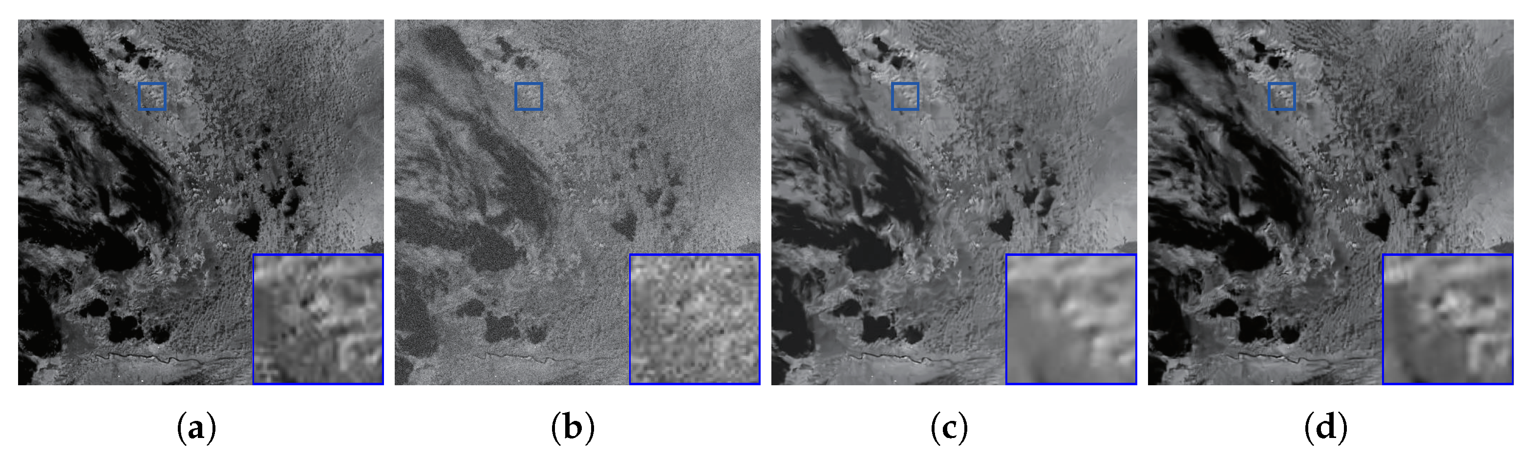
where the first term is a data fidelity term to guarantee its solution in the degradation process, the second term is a regularization prior formed by the properties of the latent image x to ensure its optimal approximation solution, and is a weighting parameter to balance the two terms. The most commonly used model is designated as total variation (TV), first proposed by Rudin et al. [9], which penalizes the -norm on the global gradient as a constraint. Then, some other TV-based strategies [10,11,12,13,14,15,16] were proposed to improve the denoising performance with different handcrafted priors to deal with different inverse problems. However, these TV-based methods have some problems: First, their results are sensitive to the selection of a set of parameters and may produce “staircase” results. Second, they may smooth preferable structures due to the piecewise constant assumption. More importantly, these TV-based methods have a heavy computational burden. Figure 1 shows a visual comparison between a model-based scheme and the proposed MD approach, from which we can observe that the denoising performance of the model-based approach is still to be improved and many rich structures in its result are over-smoothed. Unfortunately, it requires more than 780 s of computational time, which is undesirable for its extensive applications.
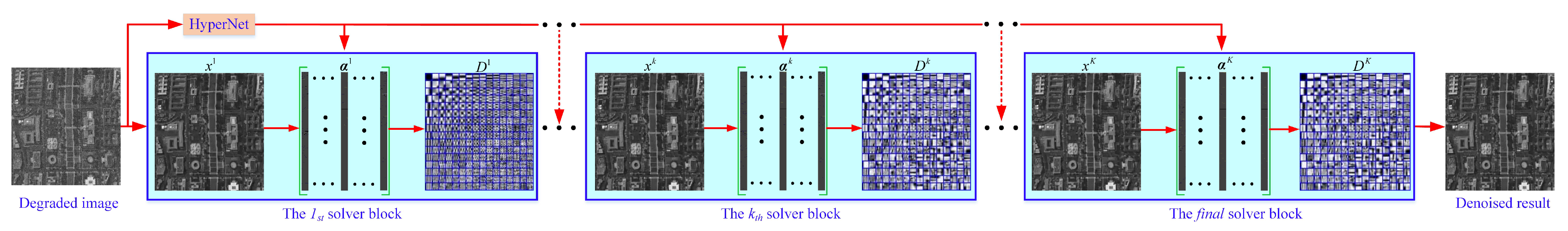
To improve the efficiency, as well as to have a competitive denoising performance, we further studied the sparse coding model and found that its two subproblems decomposed by the alternating direction method of multipliers (ADMM) [17] are pure AWGN removal problems. As mentioned in [18,19,20,21], such pure AWGN removal problems can be replaced by deep denoisers due to their high flexibility, high efficiency, and powerful modeling capacity. As such, two deep denoiser priors, acting as two independent modulars, are proposed to be plugged into the iterative optimization process of the unfolding sparse COMM to speed up its convergence to a promising approximation solution. The flowchart of the proposed framework is shown in Figure 2.
Our main contributions are summarized as follows:
- We propose a novel sparse coding denoising strategy, namely model-driven deep denoising (MD), for the pursuit of pleasing denoising performance efficiently.
- A learnable iterative soft thresholding algorithm (LISTA) is proposed for pursing the solution of sparse coding coefficient, while a lightweight residual network for learning a dictionary.
- The quantitative and qualitative results of experiments on both synthetic and real-life remote sensing images validate that the proposed MD approach is effective and even outperforms the state-of-the-art methods.
The remaining parts of our work are organized as follows. Section 2 briefly reviews the previous related work. Section 3 reports the proposed model-driven deep denoising (MD) strategy and its optimization. Section 4 provides the quantitative and qualitative experimental results. We summarize our work in Section 5.
2. Related Works
In this section, three categories of the previous methods, including sparse-model-based handle-crafted image priors, discriminative learning strategies, and model-guided deep convolutional neural networks (deep unfolding), are briefly introduced.
2.1. Sparse-Model-Based Handle-Crafted Image Priors
Inspired by the performance of BM3D, researchers further studied the neighboring stacked patches having a non-local self-similar (NSS) property that can be further transformed into various forms for model construction. One is low-rank regularization, such as Dong et al. [22], who proposed nonlocal low-rank regularization for compressive sensing. Yang et al. [23] presented a field of expert-regularized nonlocal low-rank matrix approximation (RFoE) denoising models. To make the rank estimation more accurate and obtain a preferable solution, Xue et al. [24] explored two intrinsic priors, including the global correlation across spectrum (GCS) and nonlocal self-similarity (NSS) over space, to avoid tensor rank estimation bias for denoising performance. Liu et al. [25] developed a multigraph-based low-rank tensor approximation for hyperspectral image restoration. Similar to TV problems, the above low-rank matrix factorization (LRMF) problems are also nonconvex optimization problems. There is another direction of research for low-rank matrix approximation: nuclear norm minimization (NNM) [26]. Compared to non-convex LRMF problems, it is the tightest convex relaxation with a certain data fidelity term, so it has attracted great attention and has been extended to many approaches, such as weighted NNM (WNNM) [27], weighted Schatten p-norm minimization (WSNM) [28], and the iterative weighted nuclear norm (IWNN) [29]. These methods assign higher weights to larger singular values, which are flexible for coping with different rank components and generate better approximation solutions than the LRMF problems [30]. Additionally, some methods [31,32,33,34,35] have combined nonlocal low-rank tensor decomposition and total variation regularization for the pursuit of high hyperspectral image denoising performance.
There is also another strategy to represent the non-similar stacked patch, which can be approximated by sparse coding coefficients with a redundant dictionary [36,37,38]. As traditional dictionaries are manually designed and are not flexible in representing the complex image structures, they are commonly learned directly from image data to develop dictionary learning (DL) methods. In sparse DL methods, k-singular-value decomposition (K-SVD) is a well-known approach to alternatively update the sparse coding and dictionary [39]. However, it lacks a shift-invariance property. To cope with this issue, convolutional dictionary learning (CDL) [40,41] replaced matrix multiplication with the convolution operation in signal representation. Inspired by CDL, many CDL-based methods have been proposed and have achieved considerable progress in improving denoising performance [42,43,44,45,46,47,48,49,50]. For instance, convolutional sparse coding (CSC) [42] is proposed to solve the sparse coding problem. Dong et al. [43] proposed a nonlocally centralized sparse representation (NCSR) with the usage of nonlocal self-similar patches for image restoration. Xu et al. [47] developed a trilateral weighted sparse coding (TWSC) strategy by introducing three weight terms into the sparse coding framework. From a multi-scale perspective, an image is separated into high- and low-frequency components, and then, the sparse representation is reconstructed using patch-based structure similarity and singular-value decomposition (SVD) [49]. Ou et al. [50] used multi-scale NSS priors to construct patch groups and proposed a multi-scale weighted group sparse coding model (MS-WGSC) for image denoising with ringing artifact removal while preserving rich details. These methods employ the advantages of the high-order dependency of sparse coefficients for pleasing denoising performance. However, they have their own drawbacks: the weak model representation flexibility of the universal dictionary, several regularization parameters that are required to be manually set, and even a heavy computational time burden.
2.2. Deep Neural Network
In recent years, deep neural network (DNN) approaches have been popularly developed to directly learn a nonlinear mapping function from the space of noisy images to that of clean images [51]. With the employment of its strong learning capacity on large training samples, many DNN-based denoising methods have been proposed [18,19,20,21,52,53,54,55,56,57,58,59,60,61,62,63]. For example, Chen et al. [52] used a loss-based scheme to learn filters from training data and formed a trainable nonlinear reaction diffusion (TNRD) model. Zhang et al. [18] proposed a classical deep image denoising strategy, which is named the deep convolutional neural network (DnCNN), and then proposed a fast and flexible solution for CNN-based image denoising (FFDNet) [21]. Guo et al. [53] presented a convolutional blind denoising network (CBDNet) by incorporating the network architecture, noise modeling, and asymmetric learning to improve the robustness and practicability of deep denoising models. Jia et al. [54] developed a fractional optimal control network (FOCNet) for image denoising. Tian et al. [55] integrated batch renormalization into a deep CNN (DCNN) to obtain good results. Zhang et al. [56] used a memory-efficient hierarchical neural architecture to search for pleasing solutions. COLA-Net [57] and SQAD [58] introduced an attention mechanism into the DNN for denoising performance improvement. The residual network was further extended by Zhang et al. [59] to a residual dense network. Non-local self-similarity [60] and the low rank [25] of stacked patches are both plugged into a convolutional neural network for noise removal. Jia et al. [61], Dong et al. [62], and Xu et al. [63] reduced noise using deep learning technologies from a multi-scale perspective.
The above methods successfully and efficiently achieved leading denoising performance due to their powerful learning capabilities and surpassed the traditional image denoising methods by learning the image denoisers from the training data. However, these DNN-based methods lack good interpretability because they directly map low-quality images to latent noise-free results with a black-box nature, and their application range is greatly limited because they are usually applied to a specialized task.
2.3. Deep Unfolding
To address the above issues of DNN-based methods, deep learning technologies are usually exploited to complete specialized tasks (e.g., denoisers) in the optimization process of sparsity-based models, which can be decoupled by certain algorithms (such as the alternating direction method of multipliers (ADMM) [17] and half-quadratic splitting (HQS) [64]). For instance, Meinhardt et al. [65] replaced the proximal operator of regularization with a denoising neural network. The methods in [66,67,68] unfolded the CSC process and integrated DNN into the CSC problem for an efficient solution. Simon et al. [69] further improved it by using strided convolution. Dong et al. [70] unfolded the iterative process into a feed-forward neural network. Fu et al. [71] proposed a multi-scale feature extraction module for reducing JPEG artifacts. Bertocchi et al. [72] provided a neural network architecture by unfolding a proximal interior point algorithm. Zheng et al. [73] proposed a deep convolutional dictionary learning (DCDicL) framework to learn the priors for both representation coefficients and dictionaries. Sun et al. [74] used low-rank representation and a CNN denoiser (LRR-CNN) to form a hyperspectral image denoising model. Huang et al. [75] proposed a nonlocal self-similar (NSS) block-based deep image denoising scheme, designated the deep low-rank prior (DLRP), to achieve efficient performance. Xu et al. [76] developed an end-to-end deep architecture to follow the process of sparse-representation-based image restoration.
These unfolding iterative denoising strategies successfully improved their interpretability when compared to DNN-based methods. However, the existing deep unfolding methods also have drawbacks as follows: (1) the learning capacity of DNNs is wasted with the usage of fixed priors (without learning the priors from data). (2) The dictionary is universally learned and is not adaptive, resulting in their performance being even lower than that of DNN-based approaches.
3. Model-Driven Deep Denoising
3.1. MD Model Generation
For an exemplar patch of size at position i denoted by , its similar neighborhood patches are ordered lexicographically to construct a data matrix:
where () is a column vector similar to and m is the total number of similar patches that are selected by the following criteria:
where is the position set of similar patches and is a judgment parameter (which is empirically set as 0.4 in the following experiments), and , the correlation coefficient between the i-th patch and the j-th patch, is computed by
where is a function to compute the mean value of a matrix. Generally, this constructed data matrix is sparse and can be characterized by a coding coefficient vector with a given or learned dictionary D [75]. That is, . Compared to the usage of a given dictionary, a learned dictionary is more flexible to be able to adaptively interpret complex structures. By considering the above constraints and the priors on the unknown variables, we can construct a global objective model as follows:
where , is a penalty parameter (which has a direct relationship with the noise level ), while and are regularization parameters to guarantee that the model has an optimized solution.
3.2. MD Model Optimization
The objective function (6) can be decomposed into the following two subproblems and be solved by alternately minimizing them for the latent clean image x, the sparse representation matrix , and dictionary D while keeping the other variables fixed:
3.2.1. Solving x
In the -th iteration, Sub-problem (7a) for x is a quadratic optimization problem and has a fast closed-form solution:
where I is a unit matrix and is the transpose matrix of .
3.2.2. Solving and D
By the usage of the alternating direction method of multipliers (ADMM), Sub-problem (7b) can be further separated into two independent subproblems as follows:
where the sparse coding is estimated by Equation (9a) from with a fixed dictionary D. Alternately, dictionary D is computed by Equation (9b) from with a known sparse coding :
- For sparse coding : Equation (9a) is a restoration task for from , which can be rewritten as
The traditional strategies to construct the sparse coding model usually plug the handle-crafted priors into Problem (10). Specifically, is an -norm, which is an original sparse approximation problem to count the number of non-zero elements in . Unfortunately, the -norm is an N-P problem that is difficult to solve. An -norm () is usually employed to replace the -norm to form a convex and continuous problem, with which Problem (10) is equivalently written as
which can be effectively solved by a popularly representative approach, the iterative soft thresholding algorithm (ISTA) [77], to guarantee its convergence. The solution of the iterative process at the k-th iteration using the ISTA is
where and is a parameter that should meet the following criterion: , where is the largest eigenvalue of . is an elementwise soft-thresholding shrinkage function, which is defined as
to search for the global minimum of the sparse representation model (10). However, this global minimum solution is dependent on the selection of parameters and . Moreover, the obtained solution of the -norm is theoretically approximated to the desired solution of the -norm, but it is not an exact solution and depends on its sparsity and the properties of dictionary D. Actually, the iterative process in Equation (11) can be equivalently written as
Let and , then Equation (14) can be simplified as
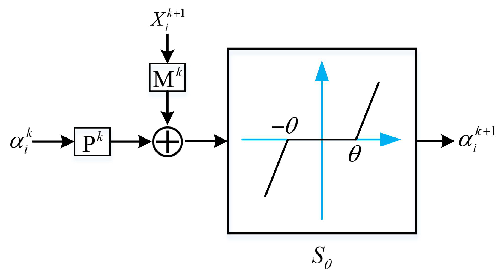
which can be implemented by a learnable ISTA (LISTA) encoder network to obtain a fast sparse coding approximation solution of Equation (10). The LISTA encoder network is viewed as a modular part to be plugged into the denoising model, where the thresholding parameter is learned for the pursuit of the sparse coding , which is then fixed for solving other variables. The framework of the LISTA encoder for Problem (15) is shown in Figure 3.
- For dictionary D: with the aid of the half-quadratic splitting (HQS) algorithm due to its simplicity and fast convergence in many applications. Equation (9b) can be solved by inducing an auxiliary variable to convert the constrained problem (9b) into an unconstrained one:
By employing ADMM, Equation (16) is decomposed into the following two independent problems:
Similar to solving x in Equation (7a), Equation (17a) also has a closed-form solution:
The subproblem (17b) can be further modified as
which is a common Gaussian noise removal issue on with a noise level . For simplicity, it is replaced by a learned deep Gaussian denoiser (DGD) as follows:
Compared to the traditional approaches with handle-crafted priors , the DGD has several advantages. First, the unknown image prior can be implicitly replaced by any Gaussian denoiser. Second, the learned DGD can be jointly utilized as a modular part to efficiently solve many inverse problems due to its high flexibility and powerful modeling capacity.
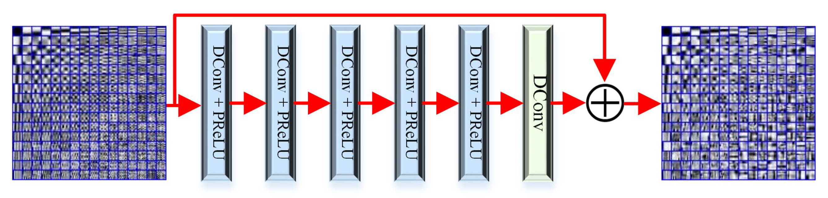
Figure 4 shows the architecture of the deep dictionary network (DDNet) . As D has a lighter structure derived from a deep residual network [78], we designed a simple network whose receptive field and learning capability are sufficient to generate a pleasing result. As shown in Figure 4, DDNet has six layers, including five “DConv + PReLU” layers and one “DConv” layer. DConv preserves the merits of while enlarging the receptive field [79]. PReLU is a parameterized nonlinearity function to generate a high-quality estimation with few filters [80]. The number of channels in each layer is 16.
4. Experimental Results and Analysis
4.1. Experimental Preparation
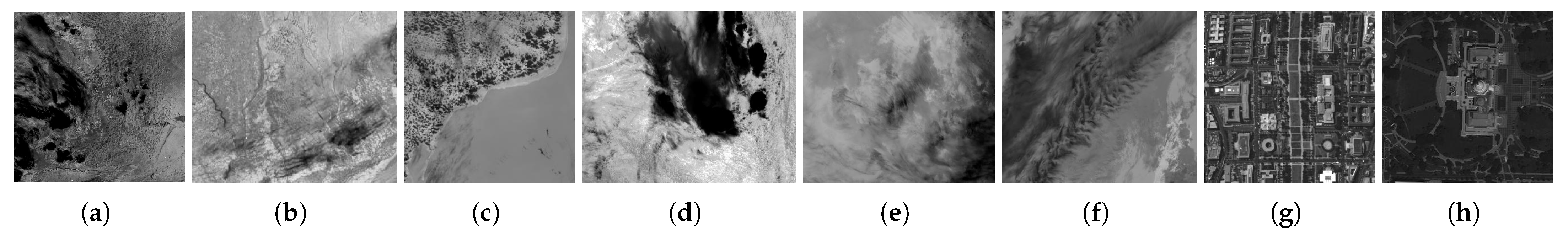
In this section, we present the experiments conducted on both synthetic and real-life RSIs by state-of-the-art methods to obtain quantitative and qualitative results, which were employed to validate the effectiveness of the proposed MD. All comparable approaches were tested on a PC with an Intel Core i7-5960X CPU 3.0 GHz 16.0 GB memory and a GeForce RTX 2080Ti GPU, and the MATLAB 2014b software was used for the model-based methods, while the TensorFlow software package was exploited for the deep learning methods. All training and testing images were downloaded from [81,82], which were randomly cropped into 735,602 patches of size with a ratio of 7:3. Note that hyperspectral images were treated as common RSI images in a band-by-band manner to be proceeded. The Adam optimizer [83,84] was used to minimize the loss function, which was adopted to generate the optimization network parameters shared in each stage. The block size was , while the dictionary size was . The learning rate started from 1e-4, decayed by half every 1e5 iterations, and finally, ended after 100 epochs. The noise level ranged from 1 to 50 with a step size of 1, which is enough for training a set of deep denoisers. The iterative optimization process is finished when the following criterion is satisfied: . Eight selected test images (as shown in Figure 5) from different datasets were experimented on and presented in this section to verify the effectiveness of the proposed MD strategy. For similarity, the eight test images were named MODIS-A1, MODIS-A2, MODIS-A3, MODIS-T1, MODIS-T2, MODIS-T3, Hyper-WDCM, and Multi-WDC.
Parameters setting: The unknown parameters referred to in Section 3 include four regularization factors and the iteration number K. In order to make the proposed MD method image adaptive, a HyperNet module, taking noise level as the inputs, was exploited to learn the four hyper-parameters for each stage. There are two Conv layers with kernel size 1 and a SoftPlus layer to allow regularization parameters to be positive in the HyperNet module. For noise level , the initial value was known in the testing experiments, but it was unknown at other stages and in the experiments on real-life RSIs. To address this issue, we estimated it at each stage by the method presented in [85] to ensure the alternating iterations adaptively converged to a fixed point. The initial D was the DCT dictionary and .
Quantitative index selection: Except for subjective evaluation, we, in the simulated experiments, employed the peak-signal-to-noise ratio (PSNR) and structural similarity index measure (SSIM) to objectively assess the capacity of the state-of-the-art in AWGN removal and structural preservation, respectively [73]. In real-world experiments, two reference-free metrics, the Q-metric (QM) [4] and natural image quality evaluator (NIQE) [86], were used to evaluate their ability to preserve fine structures and improve estimated image quality, respectively. The higher the PSNR is, the better the AWGN noise suppression. The larger the SSIM and the QM are, the richer the structures. The smaller the NIQE is, the better the denoised image quality.
Comparison approaches’ selection: To check the effectiveness of the proposed MD scheme and its advantages, three types of methods described in Section 2, model-based (NCSR [43] and WSSR [6]), DNN-based ([18]), and deep-unfolding-based (DKSVD [68], DCDicL [73], LRR-CNN [74], and DLRP [75]), were selected to be utilized, and their results were compared regarding quantization and qualification.
4.2. Analysis of Convergence and Intermediate Results
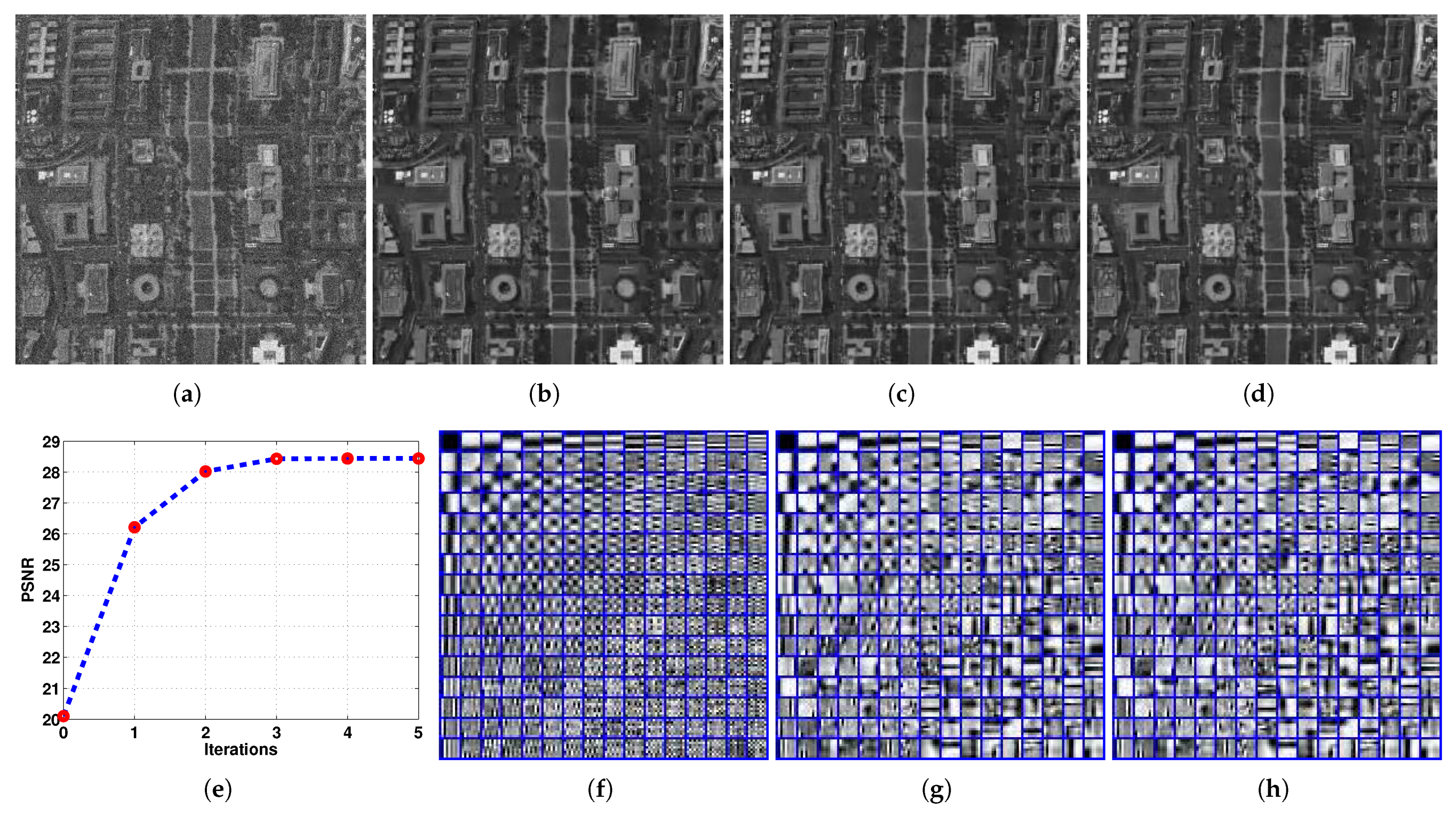
Figure 6 presents the intermediate results generated by the proposed MD method and its convergence on the Hyper-WDCM image with Noise Level 20. With the aid of two learned strategies (including the LISTA encoder and DDNet), the noise in the estimated image (as shown in Figure 6b–d) was more effectively suppressed with the increment of the iterations, while the atoms in the adaptive estimated dictionary (as shown in Figure 6f–h) were much closer to the units of the ground-truth image. The convergence result in Figure 6e shows that the MD method quickly converged to a fixed point with only five iterations, indicating that the two powerful learning modules explored in the optimization process of our method can effectively help it speed up to an enjoyable solution.
4.3. Experiments on the Synthetic RSI Images
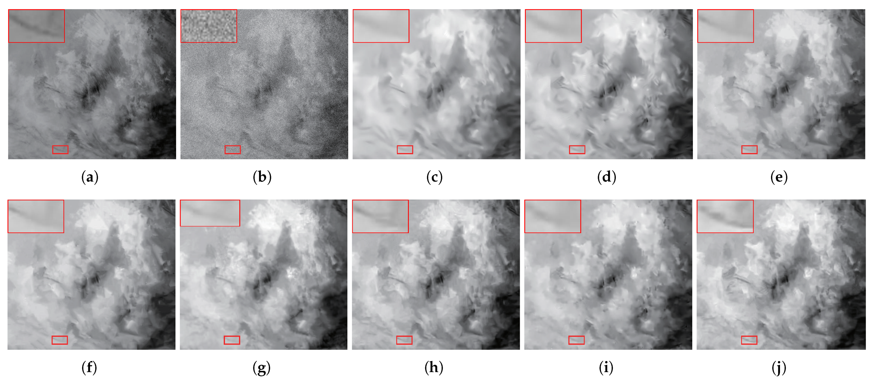
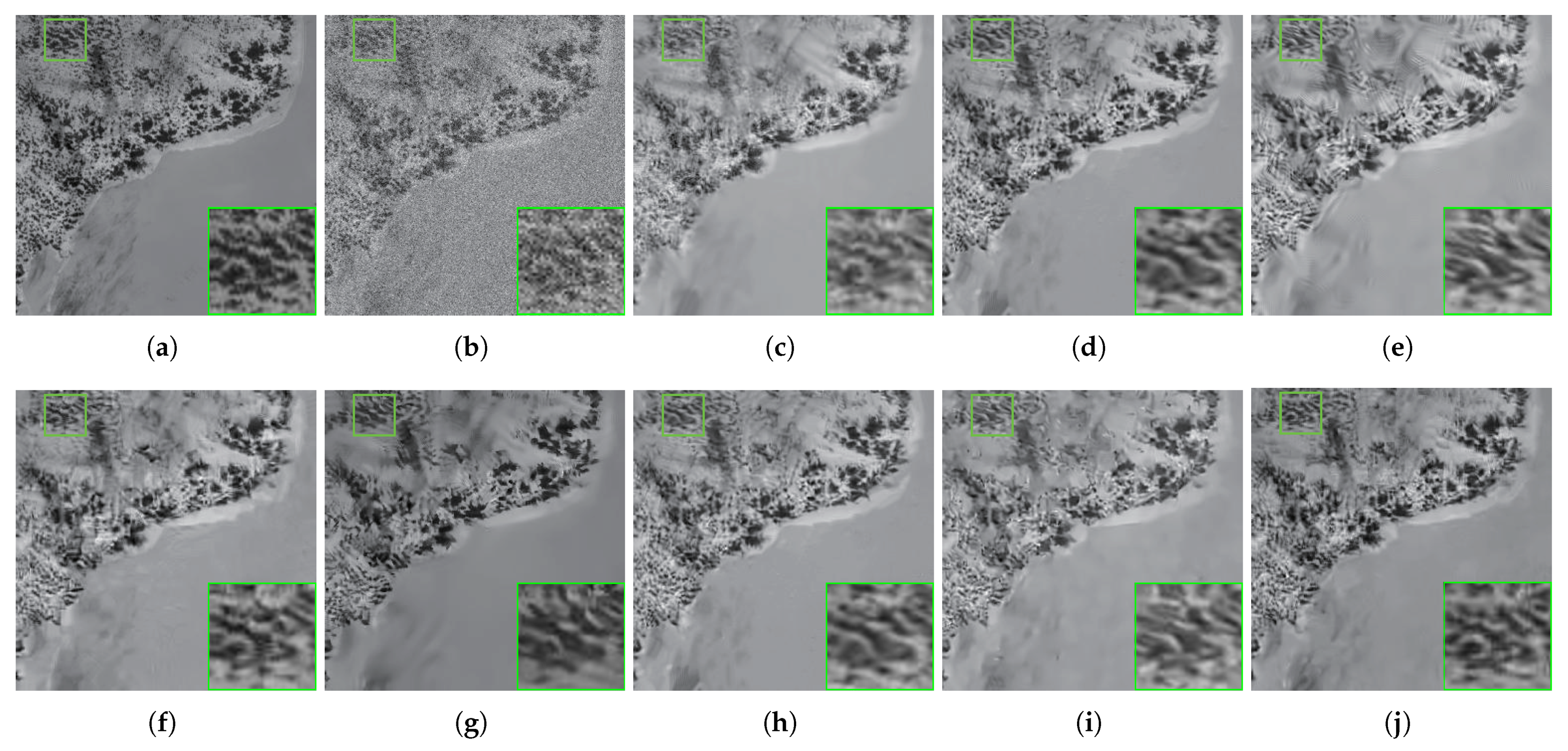
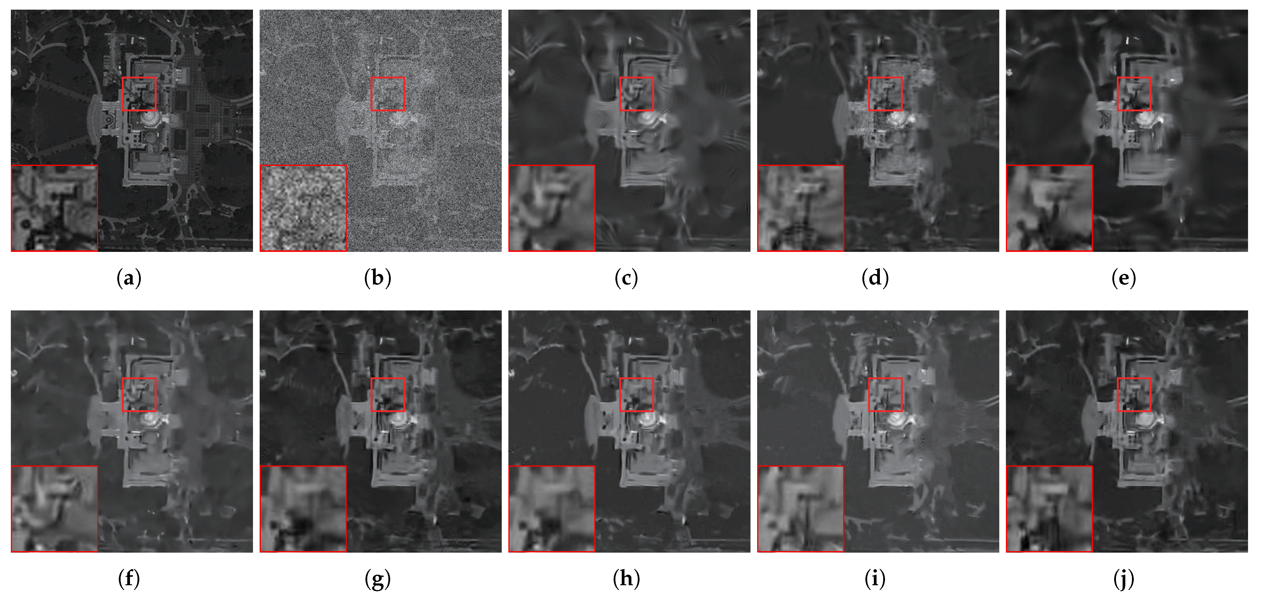
The eight synthetic RSI images shown in Figure 5 were simulated and tested to examine the effectiveness of the MD method. Three respective visual comparisons with different noise levels are presented in Figure 7, Figure 8 and Figure 9. By observing these results, we found that NCSR produced the worst maps with distorted structures. WSSR pursues better results with richer textures than the NCSR’s images at the cost of a z huge time burden. DnCNN directly removes noise with the usage of a learned black-block mapping function and produces enjoyable results; however, its interpretability is ambiguous. The deep unfolding methods (DKSVD, DCDicL, LRR-CNN, and DLRP) enhance the interpretability of the DNN and assign its specialized task, but their results are over-smoothed, which are even worse than those produced by DnCNN. The reason may be that there are too many regularization parameters that are not adaptive. In contrast, the details generated by the proposed MD method are better highlighted and are closer to those of the ground-truth images.
The objective values of PSNR and SSIM are shown in Table 1 and Table 2, respectively, from which some observations can be made. First, MD obtains an enjoyable PSNR and SSIM on all RSI images at each noise level, indicating that MD can yield competitive denoising performance and preferable results with plentiful structures. Second, MD generates the best average PSNR, which outperforms the second-best method (deep unfolding DLRP) from 0.18 dB to 0.39 dB, verifying that MD is effective at noise removal. Such conclusions are consistent with the visual comparisons.
4.4. Experiments on Real-World RSI Images
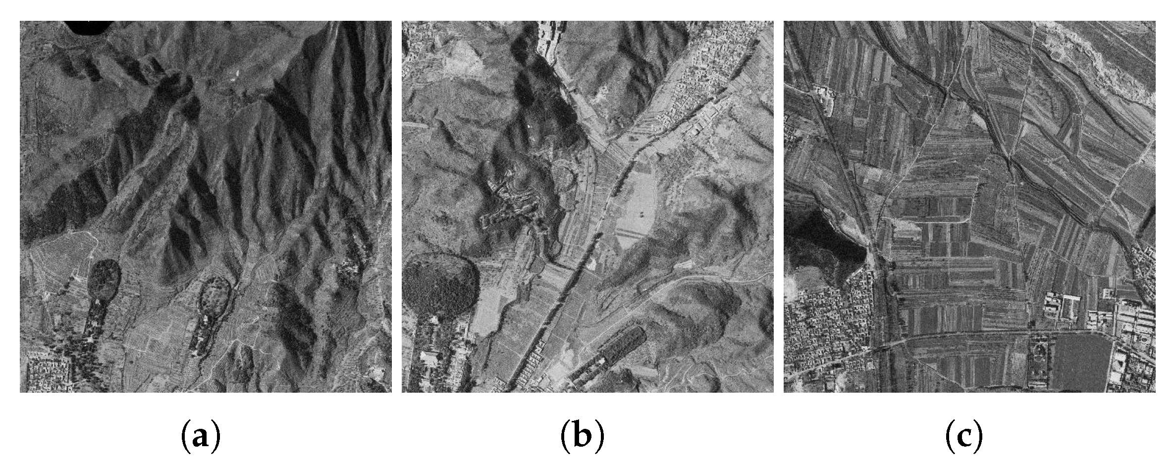
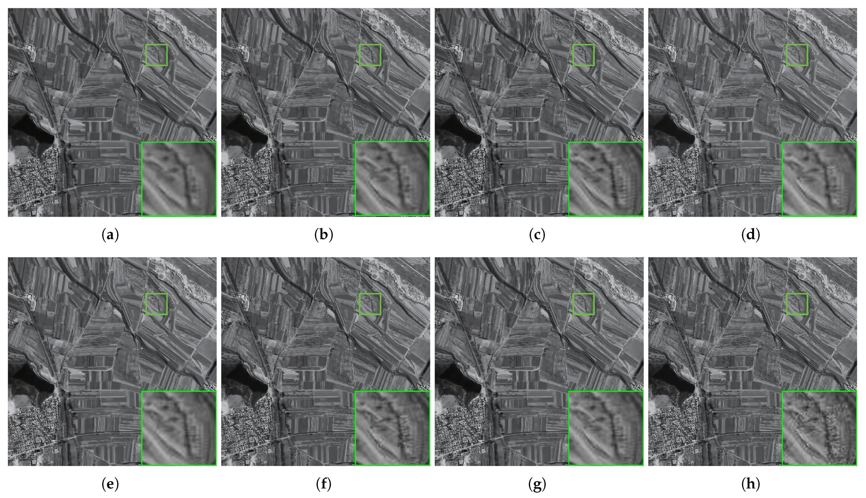
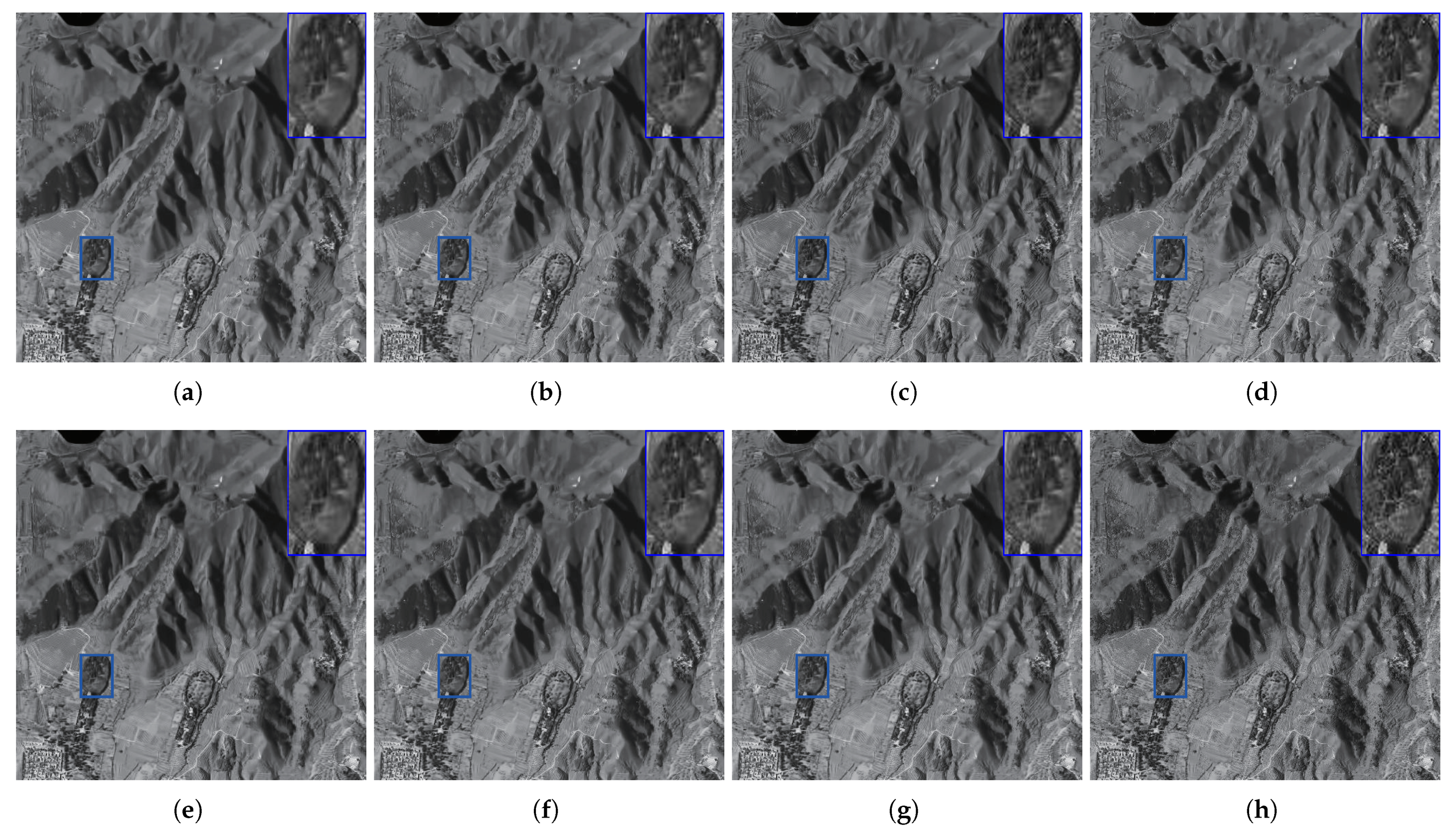
To further examine its advantages, we also applied the state-of-the-art to real-world RSI images (as shown in Figure 10), which are also related in [6]. Their denoised results are compared in Figure 11 and Figure 12, in which we can observe that the details in the results produced by MD are much richer than those generated by the competing methods (the readers can visualize the enlarged parts in these figures by themselves). Meanwhile, the quantitative comparisons are presented in Table 3. For each real-life RSI image, MD achieves the highest QM value, further demonstrating that MD performs extraordinarily well on preferable detail preservation. This is because MD perceives the global information from the input images with an adaptive learning dictionary, making it image-adaptive. More importantly, each result denoised by MD has the smallest NIQE value, validating that its quality is the most comfortable for human visualization.
4.5. Computational Complexity
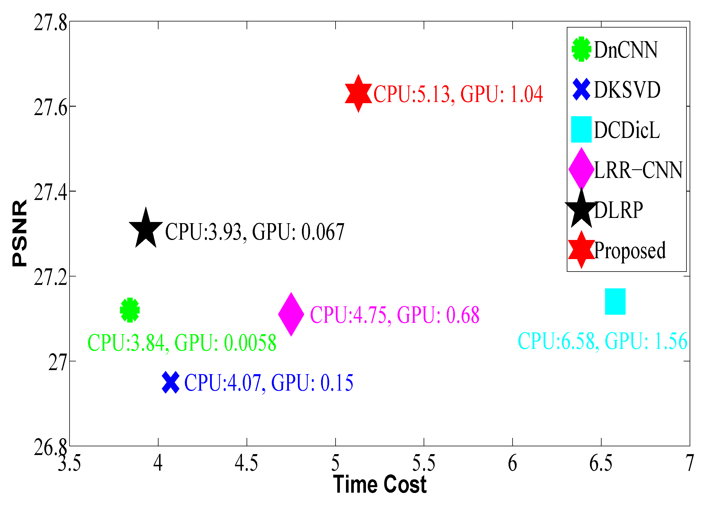
Efficiency is also an important index to evaluate the possibility for extensive applications. As model-based methods have a high time burden (CPU time), which may be 100-times more than those produced by deep-learning-based approaches, they were not selected for efficiency assessment. Figure 13 shows a testing example on the MODIS-A1 image with size , from which we can see that MD is slower than DnCNN, DKSVD, LRR-CNN, and DLRP, but is faster than DCDicL with a complex solution process. However, their denoising performance lags behind that of MD.
In sum, taking all comparisons into account, MD with two deep learning modulars is image-adaptive, can effectively and efficiently obtain a stable solution, and is suitable for extensive applications.
5. Conclusions
In the RSI image denoising task, there are three well-known key points, denoising performance, structure preservation, and efficiency, that should all be considered in designing a good interpretability strategy. To address these issues, this paper reported a deep unfolding scheme, namely model-driven deep denoising (MD), including the following: (1) The MD model was constructed with the rearranged self-similar data matrix, having sparse coding and a learned dictionary. (2) The MD model was separated into two independent subproblems, including the data fidelity term (which has a closed-form solution) for the latent clean image and the regularization term for the sparse coding and dictionary, by using the alternating direction method of multipliers (ADMM). (3) With further separation of the regularization term, the regularization problem was decomposed into two independent subproblems, respectively, for the sparse coding and dictionary. The sparse coding problem was solved by the proposed learnable ISTA (LISTA) encoder network, while the dictionary was learned by a lightweight residual network (namely the deep dictionary network (DDNet)) for adaptive images. (4) The two deep neural networks, acting as two modulars, were plugged into the iterative procedure to speed up the optimization process for a fixed solution. Finally, the proposed MD, as well as the state-of-the-art were evaluated on both synthetic and real-life RSI images, for which the comparison results for the quantitation and qualification validated that it is effective at improving the denoising performance and preserving rich structures. Its satisfactory computation time is beneficial for its extensive application.
Author Contributions
Z.H.: investigation, writing—original draft. Z.Z. and Y.Z.: software. Z.W. and B.X.: visualization, investigation. J.L. and S.L.: writing—review and editing. H.F.: conceptualization, methodology. All authors have read and agreed to the published version of the manuscript.
Funding
This work was supported in part by the National Natural Science Foundation of China under Grant No. 61901309.
Data Availability Statement
Not applicable.
Acknowledgments
We appreciate the critical and constructive comments and suggestions from the Reviewers, which helped improve the quality of this manuscript.
Conflicts of Interest
The authors declare no conflict of interest.
References
- Li, Y.; Zhang, Y.; Zhu, Z. Error-tolerant deep learning for remote sensing image scene classification. IEEE Trans. Cybern. 2021, 51, 1756–1768. [Google Scholar] [CrossRef] [PubMed]
- Li, Y.; Zhang, Y. A new paradigm of remote sensing image interpretation by coupling knowledge graph and deep learning. Geomatics Inf. Sci. Wuhan Univ. 2022, 47, 1176–1190. [Google Scholar] [CrossRef]
- Huang, Z.; Zhang, Y.; Li, Q.; Zhang, T.; Sang, N.; Hong, H. Progressive dual-domain filter for enhancing and denoising optical remote sensing images. IEEE Geosci. Remote Sens. Lett. 2018, 15, 759–763. [Google Scholar] [CrossRef]
- Chang, Y.; Chen, M.; Yan, L.; Zhao, X.; Li, Y.; Zhong, S. Toward universal stripe removal via wavelet-based deep convolutional neural network. IEEE Trans. Geosci. Remote Sens. 2020, 58, 2880–2897. [Google Scholar] [CrossRef]
- Rasti, B.; Chang, Y.; Dalsasso, E.; Denis, L.; Ghamisi, P. Image restoration for remote sensing: Overview and toolbox. arXiv 2021, arXiv:2107.00557. [Google Scholar] [CrossRef]
- Huang, Z.; Zhang, Y.; Li, Q.; Li, X.; Zhang, T.; Sang, N.; Hong, H. Joint analysis and weighted synthesis sparsity priors for simultaneous denoising and destriping optical remote sensing images. IEEE Trans. Geosci. Remote Sens. 2020, 58, 6958–6982. [Google Scholar] [CrossRef]
- Buades, A.; Coll, B.; Morel, J. A non-local algorithm for image denoising. In Proceedings of the 2005 IEEE Computer Society Conference on Computer Vision and Pattern Recognition (CVPR’05), San Diego, CA, USA, 20–25 June 2005; Volume 2, pp. 60–65. [Google Scholar]
- Dabov, K.; Foi, A.; Katkovnik, V.; Egiazarian, K. Image denoising by sparse 3-D transform-domain collaborative filtering. IEEE Trans. Image Process. 2007, 16, 2080–2095. [Google Scholar] [CrossRef]
- Rudin, L.; Osher, S.; Fatemi, E. Nonlinear total variation based noise removal algorithms. Physica D 2007, 60, 259–268. [Google Scholar] [CrossRef]
- Bougleux, S.; Peyré, G.; Cohen, L. Non-local regularization of inverse problems. Inverse Probl. Imaging 2011, 5, 511–530. [Google Scholar]
- Zuo, W.; Zhang, L.; Song, C.; Zhang, D. Texture enhanced image denoising via gradient histogram preservation. In Proceedings of the IEEE Conference on Computer Vision and Pattern Recognition (CVPR), Portland, OR, USA, 23–28 June 2013. [Google Scholar]
- Zhu, H.; Cui, C.; Deng, L.; Cheung, R.; Yan, H. Elastic Net Constraint based Tensor Model for High-order Graph Matching. IEEE Trans. Cybern. 2020, 51, 4062–4074. [Google Scholar] [CrossRef]
- Li, Z.; Malgouyres, F.; Zeng, T. Regularized non-local total variation and application in image restoration. J. Math. Imaging Vis. 2017, 59, 296–317. [Google Scholar] [CrossRef]
- Zhang, H.; Tang, L.; Fang, Z.; Xiang, C.; Li, C. Nonconvex and nonsmooth total generalized variation model for image restoration. Signal Process. 2018, 143, 69–85. [Google Scholar] [CrossRef]
- Liu, J.; Ma, R.; Zeng, X.; Liu, W.; Wang, M.; Chen, H. An efficient non-convex total variation approach for image deblurring and denoising. Appl. Math. Comput. 2021, 397, 125977. [Google Scholar] [CrossRef]
- Shen, Y.; Liu, Q.; Lou, S.; Hou, Y. Wavelet-based total variation and nonlocal similarity model for image denoising. IEEE Signal Process. Lett. 2017, 24, 877–881. [Google Scholar] [CrossRef]
- Boyd, S.; Parikh, N.; Chu, E. Distributed optimization and statistical learning via the alternating direction method of multipliers. Found. Trends® Mach. Learn. 2011, 3, 1–122. [Google Scholar]
- Zhang, K.; Zuo, W.; Chen, Y.; Meng, D.; Zhang, L. Beyond a Gaussian denoiser: Residual learning of deep CNN for image denoising. IEEE Trans. Image Process. 2017, 26, 3142–3155. [Google Scholar] [CrossRef] [Green Version]
- Zhu, H.; Qiao, Y.; Xu, G.; Deng, L.; Yu, F. DSPNet: A lightweight dilated convolution neural networks for spectral deconvolution with self-paced learning. IEEE Trans. Ind. Inform. 2019, 16, 7392–7401. [Google Scholar] [CrossRef]
- Li, Y.; Zhang, Y.; Huang, X.; Zhu, H.; Ma, J. Large-scale remote sensing image retrieval by deep hashing neural networks. IEEE Trans. Geosci. Remote Sens. 2018, 56, 950–965. [Google Scholar] [CrossRef]
- Zhang, K.; Zuo, W.; Zhang, L. FFDNet: Toward a fast and flexible solution for CNN-based image denoising. IEEE Trans. Image Process. 2018, 27, 4608–4622. [Google Scholar] [CrossRef] [Green Version]
- Dong, W.; Shi, G.; Li, X.; Ma, Y.; Huang, F. Compressive sensing via nonlocal low-rank regularization. IEEE Trans. Image Process. 2014, 23, 3618–3632. [Google Scholar] [CrossRef]
- Yang, H.; Lu, J.; Zhang, H.; Luo, Y.; Lu, J. Field of experts regularized nonlocal low rank matrix approximation for image denoising. J. Comput. Appl. Math. 2022, 412, 114244. [Google Scholar] [CrossRef]
- Xue, J.; Zhao, Y.; Liao, W.; Chan, C. Nonlocal low-rank regularized tensor decomposition for hyperspectral image denoising. IEEE Trans. Geosci. Remote Sens. 2019, 57, 5174–5189. [Google Scholar] [CrossRef]
- Liu, N.; Li, W.; Tao, R.; Du, Q.; Chanussot, J. Multi-graph-based low-rank tensor approximation for Hyperspectral image restoration. IEEE Trans. Geosci. Remote Sens. 2022, 60, 5530314. [Google Scholar]
- Donoho, D.; Gavish, M.; Montanari, A. The phase transition of matrix recovery from gaussian measurements matches the minimax mse of matrix denoising. Proc. Natl. Acad. Sci. USA 2013, 110, 8405–8410. [Google Scholar] [CrossRef] [PubMed] [Green Version]
- Gu, S.; Zhang, L.; Zuo, W.; Feng, X. Weighted nuclear norm minimization with application to image denoising. In Proceedings of the IEEE Conference on Computer Vision and Pattern Recognition, Columbus, OH, USA, 23–28 June 2014; pp. 2862–2869. [Google Scholar]
- Xie, Y.; Gu, S.; Liu, Y.; Zuo, W.; Zhang, W.; Zhang, L. Weighted schatten p-norm minimization for image denoising and background subtraction. IEEE Trans. Image Process. 2016, 25, 4842–4857. [Google Scholar] [CrossRef] [Green Version]
- Huang, Z.; Li, Q.; Fang, H.; Zhang, T.; Sang, N. Iterative weighted nuclear norm for X-ray angiogram image denoising. Signal Image Video Process. 2017, 11, 1445–1452. [Google Scholar] [CrossRef]
- Huang, T.; Dong, W.; Xie, X.; Shi, G.; Bai, X. Mixed noise removal via laplacian scale mixture modeling and nonlocal low-rank approximation. IEEE Trans. Image Process. 2017, 26, 3171–3186. [Google Scholar] [CrossRef]
- Zhang, H.; Liu, L.; He, W.; Zhang, L. Hyperspectral image denoising with total variation regularization and nonlocal low-rank tensor decomposition. IEEE Trans. Geosci. Remote Sens. 2020, 58, 3071–3084. [Google Scholar] [CrossRef]
- Zhu, H.; Ni, H.; Liu, S.; Xu, G.; Deng, L. Tnlrs: Target-aware non-local low-rank modeling with saliency filtering regularization for infrared small target detection. IEEE Trans. Image Process. 2020, 29, 9546–9558. [Google Scholar] [CrossRef]
- Li, Y.; Chen, W.; Huang, X.; Gao, Z.; Li, S.; He, T.; Zhang, Y. Mfvnet: Deep adaptive fusion network with multiple field-of-views for remote sensing image semantic segmentation. Sci. China Inf. Sci. 2022. [Google Scholar] [CrossRef]
- Zhu, H.; Zhang, J.; Xu, G.; Deng, L. Tensor field graph-cut for image segmentation: A non-convex perspective. IEEE Trans. Circuits Syst. Video Technol. 2020, 31, 1103–1113. [Google Scholar] [CrossRef]
- Kong, X.; Zhao, Y.; Xue, J.; Chan, J.C.W.; Zang, J. Hyperspectral image denoising based on nonlocal low-rank and TV regularization. Remote Sens. 2020, 12, 1956. [Google Scholar] [CrossRef]
- Li, Y.; Kong, D.; Zhang, Y.; Tan, Y.; Chen, L. Robust deep alignment network with remote sensing knowledge graph for zero-shot and generalized zero-shot remote sensing image scene classification. ISPRS J. Photogramm. Remote Sens. 2021, 179, 145–158. [Google Scholar] [CrossRef]
- Zhu, H.; Liu, S.; Deng, L.; Li, Y.; Xiao, F. Infrared Small Target Detection via Low Rank Tensor Completion with Top-Hat Regularization. IEEE Trans. Geosci. Remote Sens. 2020, 58, 1004–1016. [Google Scholar] [CrossRef]
- Li, Y.; Zhou, Y.; Zhang, Y.; Zhong, L.; Wang, J.; Chen, J. DKDFN: Domain knowledge-guided deep collaborative fusion network for multimodal unitemporal remote sensing land cover classification. ISPRS J. Photogramm. Remote Sens. 2022, 186, 170–189. [Google Scholar] [CrossRef]
- Elad, M.; Aharon, M. Image denoising via sparse and redundant representation over learned dictionaries. IEEE Trans. Image Process. 2006, 15, 3736–3745. [Google Scholar] [CrossRef] [PubMed]
- Bristow, H.; Eriksson, A.; Lucey, S. Fast convolutional sparse coding. In Proceedings of the 2013 IEEE Conference on Computer Vision and Pattern Recognition, Portland, OR, USA, 23–28 June 2013; pp. 391–398. [Google Scholar]
- Cardona, C.G.; Wohlberg, B. Convolutional dictionary learning: A comparative review and new algorithms. IEEE Trans. Comput. Imaging 2018, 4, 366–381. [Google Scholar] [CrossRef] [Green Version]
- Rey-Otero, I.; Sulam, J.; Elad, M. Variations on the CSC model. IEEE Trans. Image Process. 2020, 68, 519–528. [Google Scholar] [CrossRef]
- Dong, W.; Zhang, L.; Shi, G.; Li, X. Nonlocally centralized sparse representation for image restoration. IEEE Trans. Image Process. 2013, 22, 1620–1630. [Google Scholar] [CrossRef] [PubMed] [Green Version]
- Huang, Z.; Li, Q.; Zhang, T.; Sang, N.; Hong, H. Iterative weighted sparse representation for X-ray cardiovascular angiogram image denoising over learned dictionary. IET Image Process. 2018, 12, 254–261. [Google Scholar] [CrossRef]
- Li, Y.; Chen, W.; Zhang, Y.; Tao, C.; Xiao, R.; Tan, Y. Accurate cloud detection in high-resolution remote sensing imagery by weakly supervised deep learning. Remote Sens. Environ. 2020, 250, 112045. [Google Scholar] [CrossRef]
- Zhu, H.; Peng, H.; Xu, G.; Deng, L.; Cheng, Y.; Song, A. Bilateral weighted regression ranking model with spatial-temporal correlation filter for visual tracking. IEEE Trans. Multimed. 2021, 24, 2098–2111. [Google Scholar] [CrossRef]
- Xu, J.; Zhang, L.; Zhang, D. A trilateral weighted sparse coding scheme for real-world image denoising. In Proceedings of the European Conference on Computer Vision (ECCV), Munich, Germany, 8–14 September 2018; pp. 21–38. [Google Scholar]
- Peng, C.; Liu, Y.; Chen, Y.; Wu, X.; Cheng, A.; Kang, Z.; Chen, C.; Cheng, Q. Hyperspectral image denoising using non-convex local low-rank and sparse separation with spatial-spectral total variation regularization. arXiv 2022, arXiv:2201.02812. [Google Scholar]
- Shi, M.; Zhang, F.; Wang, S.; Zhang, C.; Li, X. Detail preserving image denoising with patch-based structure similarity via sparse representation and svd. Comput. Vis. Image Underst. 2021, 206, 103173. [Google Scholar]
- Ou, Y.; Swamy, M.N.S.; Luo, J.; Li, B. Single image denoising via multi-scale weighted group sparse coding. Signal Process. 2022, 200, 108650. [Google Scholar] [CrossRef]
- Sun, L.; Dong, W.; Li, X.; Wu, J.; Li, L.; Shi, G. Deep maximum a posterior estimator for video denoising. Int. J. Comput. Vis. 2021, 129, 2827–2845. [Google Scholar] [CrossRef]
- Chen, Y.; Pock, T. Trainable nonlinear reaction diffusion: A flexible framework for fast and effective image restoration. IEEE Trans. Pattern Anal. Mach. Intell. 2017, 39, 1256–1272. [Google Scholar] [CrossRef] [PubMed] [Green Version]
- Guo, S.; Yan, Z.; Zhang, K.; Zuo, W.; Zhang, L. Toward convolutional blind denoising of real photographs. In Proceedings of the 2019 IEEE/CVF Conference on Computer Vision and Pattern Recognition (CVPR), Long Beach, CA, USA, 15–20 June 2019; pp. 1712–1722. [Google Scholar]
- Jia, X.; Liu, S.; Feng, X.; Zhang, L. FOCNet: A fractional optimal control network for image denoising. In Proceedings of the IEEE/CVF Conference on Computer Vision and Pattern Recognition, Long Beach, CA, USA, 15–20 June 2019; pp. 6054–6063. [Google Scholar]
- Tian, C.; Xu, Y.; Zuo, W. Image denoising using deep cnn with batch renormalization. Neural Netw. 2017, 121, 461–473. [Google Scholar] [CrossRef]
- Zhang, H.; Li, Y.; Chen, H.; Shen, C. Memory-efficient hierarchical neural architecture search for image denoising. In Proceedings of the 2020 IEEE/CVF Conference on Computer Vision and Pattern Recognition (CVPR), Seattle, WA, USA, 13–19 June 2020; pp. 3657–3666. [Google Scholar]
- Mou, C.; Zhang, J.; Fan, X.; Liu, H.; Wang, R. COLA-Net: Collaborative attention network for image restoration. IEEE Trans. Multimed. 2021, 24, 1366–1377. [Google Scholar] [CrossRef]
- Pan, E.; Ma, Y.; Mei, X.; Fan, F.; Huang, J.; Ma, J. SQAD: Spatial-spectral quasi-attention recurrent network for hyperspectral image denoising. IEEE Trans. Geosci. Remote Sens. 2022, 60, 1–14. [Google Scholar] [CrossRef]
- Zhang, Y.; Tian, Y.; Kong, Y.; Zhong, B.; Fu, Y. Residual dense network for image restoration. IEEE Trans. Pattern Anal. Mach. Intell. 2021, 43, 2480–2495. [Google Scholar] [CrossRef] [PubMed] [Green Version]
- Wang, Z.; Ng, M.K.; Zhuang, L.; Gao, L.; Zhang, B. Nonlocal self-similarity-based hyperspectral remote sensing image denoising with 3-D convolutional neural network. IEEE Trans. Geosci. Remote Sens. 2022, 60, 1–17. [Google Scholar] [CrossRef]
- Jia, X.; Peng, Y.; Ge, B.; Li, J.; Liu, S.; Wang, W. A multi-scale dilated residual convolution network for image denoising. Neural Process. Lett. 2022. [Google Scholar] [CrossRef]
- Dong, X.; Lin, J.; Lu, S.; Wang, H.; Li, Y. Multiscale spatial attention network for seismic data denoising. IEEE Trans. Geosci. Remote Sens. 2022, 60, 1–17. [Google Scholar] [CrossRef]
- Xu, J.; Deng, X.; Xu, M. Revisiting convolutional sparse coding for image denoising: From a multi-scale perspective. IEEE Signal Process. Lett. 2022, 29, 1202–1206. [Google Scholar] [CrossRef]
- Zhang, K.; Gool, L.-V.; Timofte, R. Deep unfolding network for image super-resolution. In Proceedings of the 2020 IEEE/CVF Conference on Computer Vision and Pattern Recognition (CVPR), Seattle, WA, USA, 13–19 June 2020; pp. 3217–3226. [Google Scholar]
- Meinhardt, T.; Moeller, M.; Hazirbas, C.; Cremers, D. Learning proximal operators: Using denoising networks for regularizing inverse imaging problems. In Proceedings of the 2017 IEEE International Conference on Computer Vision (ICCV), Venice, Italy, 22–29 October 2017; pp. 1799–1808. [Google Scholar]
- Sreter, H.; Giryes, R. Learned convolutional sparse coding. In Proceedings of the IEEE International Conference on Acoustics, Speech and Signal Processing (ICASSP), Calgary, AB, Canada, 15–20 April 2018; pp. 2191–2195. [Google Scholar]
- Zhu, H.; Zhang, J.; Xu, G.; Deng, L. Balanced ring top-hat transformation for infrared small-target detection with guided filter kernel. IEEE Trans. Aerosp. Electron. Syst. 2021, 56, 3892–3903. [Google Scholar] [CrossRef]
- Scetbon, M.; Elad, M.; Milanfar, P. Deep K-SVD Denoising. IEEE Trans. Image Process. 2021, 30, 5944–5955. [Google Scholar] [CrossRef]
- Simon, D.; Elad, M. Rethinking the csc model for natural images. Adv. Neural Inf. Process. Syst. 2019, 32, 2274–2284. [Google Scholar]
- Dong, W.; Wang, P.; Yin, W.; Shi, G.; Wu, F.; Lu, X. Denoising prior driven deep neural network for image restoration. IEEE Trans. Pattern Anal. Mach. Intell. 2019, 40, 2305–2318. [Google Scholar] [CrossRef] [Green Version]
- Fu, X.; Zha, Z.J.; Wu, F.; Ding, X.; Paisley, J. Jpeg artifacts reduction via deep convolutional sparse coding. In Proceedings of the 2019 IEEE/CVF International Conference on Computer Vision (ICCV), Seoul, Republic of Korea, 27 October–2 November 2019; pp. 2501–2510. [Google Scholar]
- Bertocchi, C.; Chouzenoux, E.; Corbineau, M.C.; Pesquet, J.C.; Prato, M. Deep unfolding of a proximal interior point method for image restoration. Inverse Probl. 2020, 36, 034005. [Google Scholar] [CrossRef] [Green Version]
- Zheng, H.; Yong, H.; Zhang, L. Deep convolutional dictionary learning for image denoising. In Proceedings of the 2021 IEEE/CVF Conference on Computer Vision and Pattern Recognition (CVPR), Nashville, TN, USA, 20–25 June 2021. [Google Scholar]
- Sun, H.; Liu, M.; Zheng, K.; Yang, D.; Li, J.; Gao, L. Hyperspectral image denoising via low-rank representation and CNN denoiser. IEEE J. Sel. Top. Appl. Earth Obs. Remote Sens. 2022, 15, 716–728. [Google Scholar] [CrossRef]
- Huang, Z.; Wang, Z.; Zhu, Z.; Zhang, Y.; Fang, H.; Shi, Y.; Zhang, T. DLRP: Learning deep low-rank prior for remotely sensed image denoising. IEEE Geosci. Remote Sens. Lett. 2022, 19, 1–5. [Google Scholar] [CrossRef]
- Xu, W.; Zhu, Q.; Qi, N.; Chen, D. Deep sparse representation based image restoration with denoising prior. IEEE Trans. Circuits Syst. Video Technol. 2022, 32, 6530–6542. [Google Scholar] [CrossRef]
- Beck, A.; Teboulle, M. A fast iterative shrinkage-thresholding algorithm for linear inverse problems. SIAM J. Imaging Sci. 2009, 2, 183–202. [Google Scholar] [CrossRef] [Green Version]
- He, K.; Zhang, X.; Ren, S.; Sun, J. Deep residual learning for image recognition. In Proceedings of the IEEE Conference on Computer Vision and Pattern Recognition (CVPR), Las Vegas, NV, USA, 27–30 June 2016; pp. 27–30. [Google Scholar]
- Yu, F.; Koltun, V. Multi-scale context aggregation by dilated convolutions. In Proceedings of the 4th International Conference on Learning Representations, San Juan, Puerto Rico, 2–4 May 2016. [Google Scholar]
- He, K.; Zhang, X.; Ren, S.; Sun, J. Delving deep into rectifiers: Surpassing human-level performance on ImageNet classification. In Proceedings of the 2015 IEEE International Conference on Computer Vision (ICCV), Santiago, Chile, 7–13 December 2015; pp. 1026–1034. [Google Scholar]
- MODIS Data. Available online: https://modis.gsfc.nasa.gov/data/ (accessed on 30 January 2018).
- A Freeware Multispectral Image Data Analysis System. Available online: https://engineering.purdue.edu/~biehl/MultiSpec/hyperspectral.html (accessed on 30 January 2018).
- Kingma, D.; Ba, J. Adam: A method for stochastic optimization. In Proceedings of the 3rd International Conference on Learning Representations, Banff, AB, Canada, 14–16 April 2014. [Google Scholar]
- Huang, Z.; Wang, L.; An, Q.; Zhou, Q.; Hong, H. Learning a contrast enhancer for intensity correction of remotely sensed images. IEEE Signal Process. Lett. 2022, 29, 394–398. [Google Scholar] [CrossRef]
- Pyatykh, S.; Hesser, J.; Zheng, L. Image noise level estimation by principal component analysis. SIAM J. Imaging Sci. 2013, 22, 687–699. [Google Scholar] [CrossRef]
- Huang, Z.; Zhu, Z.; An, Q.; Wang, Z.; Zhou, T.; Alshomrani, A. Luminance learning for remotely sensed image enhancement guided by weighted least squares. IEEE Geosci. Remote Sens. Lett. 2021, 22, 1–5. [Google Scholar] [CrossRef]
Figure 1.
An example of a visual comparison between the model-based method (WSSR) (PSNR|SSIM: 27.2 dB|0.7155) and the proposed MD approach (PSNR|SSIM: 27.63 dB|0.7352) on the MODIS-A1 image with size and noise level . (a) Ground-truth. (b) Noised. (c) WSSR [6]. (d) Proposed.
Figure 1.
An example of a visual comparison between the model-based method (WSSR) (PSNR|SSIM: 27.2 dB|0.7155) and the proposed MD approach (PSNR|SSIM: 27.63 dB|0.7352) on the MODIS-A1 image with size and noise level . (a) Ground-truth. (b) Noised. (c) WSSR [6]. (d) Proposed.

Figure 2.
The flowchart of the proposed model-driven deep remotely sensed image denoising.

Figure 3.
Framework of LISTA encoder for updating sparse coding .

Figure 4.
The flowchart of the deep dictionary network . “DConv” denotes dilated convolution, while “PReLU” represents the parametric rectified linear unit. “⨁” is a pixelwise operator used to add feature maps.
Figure 4.
The flowchart of the deep dictionary network . “DConv” denotes dilated convolution, while “PReLU” represents the parametric rectified linear unit. “⨁” is a pixelwise operator used to add feature maps.

Figure 5.
Test images. Images in (a–h) are from the Aqua MODIS dataset, Terra MODIS dataset, hyperspectral dataset, and multispectral dataset, respectively.
Figure 5.
Test images. Images in (a–h) are from the Aqua MODIS dataset, Terra MODIS dataset, hyperspectral dataset, and multispectral dataset, respectively.

Figure 6.
The convergence curve and intermediate results generated by the proposed MD method. (a) Noised (). (b) , PSNR: 26.21 dB. (c) , PSNR: 28.43 dB. (d) , PSNR: 28.44 dB. (e) Convergence. (f) . (g) . (h) .
Figure 6.
The convergence curve and intermediate results generated by the proposed MD method. (a) Noised (). (b) , PSNR: 26.21 dB. (c) , PSNR: 28.43 dB. (d) , PSNR: 28.44 dB. (e) Convergence. (f) . (g) . (h) .

Figure 7.
Visual comparison of experiments on the MODIS-T2 image. (a) Ground-truth. (b) Noised (). (c) NCSR [43]. (d) WSSR [6]. (e) DnCNN [18]. (f) DKSVD [68]. (g) DCDicL [73]. (h) LRR-CNN [74]. (i) DLRP [75]. (j) Proposed.

Figure 8.
Visual comparison of experiments on the MODIS-A3 image. (a) Ground-truth. (b) Noised (). (c) NCSR [43]. (d) WSSR [6]. (e) DnCNN [18]. (f) DKSVD [68]. (g) DCDicL [73]. (h) LRR-CNN [74]. (i) DLRP [75]. (j) Proposed.

Figure 9.
Visual comparison of experiments on the Multi-WDC image. (a) Ground-truth. (b) Noised (). (c) NCSR [43]. (d) WSSR [6]. (e) DnCNN [18]. (f) DKSVD [68]. (g) DCDicL [73]. (h) LRR-CNN [74]. (i) DLRP [75]. (j) Proposed.

Figure 10.
Three real-life noisy RSI images used for further testing. (a) Mountain. (b) City-wall. (c) Factory.
Figure 10.
Three real-life noisy RSI images used for further testing. (a) Mountain. (b) City-wall. (c) Factory.

Figure 11.
Visual comparison of experiments on the real-life Factory image. (a) NCSR [43]. (b) WSSR [6]. (c) DnCNN [18]. (d) DKSVD [68]. (e) DCDicL [73]. (f) LRR-CNN [74]. (g) DLRP [75]. (h) Proposed.

Figure 12.
Visual comparison of experiments on the real-life Mountain image. (a) NCSR [43]. (b) WSSR [6]. (c) DnCNN [18]. (d) DKSVD [68]. (e) DCDicL [73]. (f) LRR-CNN [74]. (g) DLRP [75]. (h) Proposed.

Figure 13.
Computational time vs. PSNR for different approaches on the MODIS-A1 image with size ; the noise level is 25.
Figure 13.
Computational time vs. PSNR for different approaches on the MODIS-A1 image with size ; the noise level is 25.


Table 1.
PSNR (dB) comparisons of the state-of-the-art. For each image at each level, the best result is marked with bold font.
Table 1.
PSNR (dB) comparisons of the state-of-the-art. For each image at each level, the best result is marked with bold font.
| Methods | Noise Level | Noise Level | ||||||||||||||||
|---|---|---|---|---|---|---|---|---|---|---|---|---|---|---|---|---|---|---|
| MODIS- | Hyper-WDCM | Multi-WDC | Ave. | MODIS- | Hyper-WDCM | Multi-WDC | Ave. | |||||||||||
| A1 | A2 | A3 | T1 | T2 | T3 | A1 | A2 | A3 | T1 | T2 | T3 | |||||||
| NCSR | 28.9 | 28.81 | 29.69 | 30.37 | 35.83 | 34.67 | 28.53 | 31.03 | 30.98 | 27.5 | 27.53 | 28.07 | 29 | 34.61 | 33.41 | 27.15 | 30.34 | 29.7 |
| WSSR | 29.58 | 29.32 | 30.47 | 31.21 | 36.48 | 35.32 | 29.62 | 32.63 | 31.85 | 28.22 | 28.2 | 28.94 | 29.64 | 35.27 | 34 | 27.83 | 31.4 | 30.44 |
| DnCNN | 29.39 | 29.24 | 30.37 | 31.02 | 36.32 | 35.19 | 29.5 | 32.61 | 31.71 | 28.06 | 28.06 | 28.67 | 29.44 | 35.04 | 33.9 | 27.59 | 31.1 | 30.23 |
| DKSVD | 29.36 | 29.17 | 30.22 | 30.77 | 36.21 | 35.17 | 29.49 | 32.43 | 31.6 | 27.96 | 27.94 | 28.66 | 29.41 | 35.03 | 33.85 | 27.51 | 31.04 | 30.18 |
| DCDicL | 29.45 | 29.34 | 30.33 | 30.82 | 36.41 | 35.25 | 29.52 | 32.51 | 31.7 | 28.07 | 28.06 | 28.79 | 29.55 | 35.19 | 33.97 | 27.7 | 31.19 | 30.32 |
| LRR-CNN | 29.42 | 29.38 | 30.54 | 30.89 | 36.48 | 35.27 | 29.37 | 32.57 | 31.74 | 28.11 | 28.11 | 28.87 | 29.57 | 35.24 | 33.99 | 27.75 | 31.33 | 30.37 |
| DLRP | 29.58 | 29.5 | 30.56 | 31.09 | 36.61 | 35.38 | 29.65 | 32.65 | 31.88 | 28.3 | 28.25 | 29 | 29.69 | 35.29 | 34.15 | 28.17 | 31.44 | 30.54 |
| Proposed | 29.76 | 29.72 | 30.79 | 31.25 | 36.78 | 35.63 | 29.79 | 32.87 | 32.06 | 28.54 | 28.61 | 29.37 | 29.9 | 35.66 | 34.54 | 28.44 | 31.73 | 30.85 |
| Noise level | Noise level | |||||||||||||||||
| NCSR | 26.87 | 26.95 | 27.08 | 28.18 | 33.86 | 32.7 | 25.99 | 29.55 | 28.9 | 26.03 | 26.23 | 26.08 | 27.55 | 33.25 | 31.88 | 24.8 | 28.53 | 28.04 |
| WSSR | 27.2 | 27.28 | 27.68 | 28.69 | 34.41 | 33.07 | 26.77 | 30.33 | 29.43 | 26.44 | 26.66 | 26.82 | 28.07 | 33.75 | 32.35 | 25.65 | 29.48 | 28.65 |
| DnCNN | 27.12 | 27.2 | 27.56 | 28.51 | 34.23 | 33.02 | 26.6 | 30.06 | 29.29 | 26.14 | 26.51 | 26.57 | 27.96 | 33.45 | 32.22 | 25.53 | 29.16 | 28.44 |
| DKSVD | 26.95 | 27.04 | 27.52 | 28.47 | 34.21 | 33.01 | 26.72 | 29.92 | 29.32 | 26.15 | 26.4 | 26.57 | 27.78 | 33.42 | 32.2 | 25.36 | 29.06 | 28.37 |
| DCDicL | 27.14 | 27.24 | 27.61 | 28.64 | 34.38 | 33.04 | 26.77 | 30.09 | 29.36 | 26.2 | 26.63 | 26.65 | 28.1 | 33.6 | 32.29 | 25.55 | 29.25 | 28.66 |
| LRR-CNN | 27.11 | 27.25 | 27.67 | 28.67 | 34.39 | 33.07 | 26.74 | 30.11 | 29.38 | 26.35 | 26.65 | 26.82 | 28.03 | 33.74 | 32.3 | 25.64 | 29.39 | 28.62 |
| DLRP | 27.31 | 27.32 | 27.75 | 28.81 | 34.47 | 33.16 | 26.81 | 30.32 | 29.49 | 26.47 | 26.69 | 26.83 | 28.36 | 33.79 | 32.36 | 25.7 | 29.52 | 28.72 |
| Proposed | 27.63 | 27.69 | 28.17 | 29.14 | 35.01 | 33.69 | 27.03 | 30.68 | 29.88 | 26.75 | 26.95 | 27.11 | 28.37 | 34 | 32.86 | 26 | 29.7 | 28.97 |
| Noise level | Noise level | |||||||||||||||||
| NCSR | 25.36 | 25.48 | 25.32 | 27.06 | 32.36 | 31.37 | 24.23 | 28.05 | 27.4 | 24.95 | 25.07 | 25.04 | 26.53 | 32.02 | 30.67 | 23.62 | 27.54 | 26.93 |
| WSSR | 25.85 | 26.14 | 26.11 | 27.46 | 33.06 | 31.65 | 25.08 | 28.76 | 28.01 | 25.41 | 25.6 | 25.5 | 27 | 32.46 | 31.13 | 24.26 | 28.18 | 27.44 |
| DnCNN | 25.82 | 25.89 | 25.89 | 27.25 | 32.9 | 31.5 | 24.92 | 28.45 | 27.83 | 25.13 | 25.38 | 25.26 | 26.81 | 32.17 | 31.13 | 24.02 | 27.95 | 27.23 |
| DKSVD | 25.65 | 25.77 | 25.86 | 27.24 | 32.69 | 31.48 | 24.94 | 28.39 | 27.75 | 25.08 | 25.29 | 25.18 | 26.72 | 32.11 | 30.88 | 23.89 | 27.71 | 27.11 |
| DCDicL | 25.81 | 25.98 | 25.89 | 27.43 | 32.99 | 31.51 | 25.01 | 28.51 | 27.89 | 25.34 | 25.47 | 25.31 | 26.87 | 32.34 | 31.05 | 24.11 | 28.03 | 27.32 |
| LRR-CNN | 25.83 | 26.01 | 26.08 | 27.44 | 32.99 | 31.57 | 25.04 | 28.65 | 27.95 | 25.37 | 25.41 | 25.49 | 26.93 | 32.36 | 31.11 | 24.21 | 28.07 | 27.37 |
| DLRP | 25.95 | 26.19 | 26.15 | 27.5 | 33.16 | 31.66 | 25.12 | 28.87 | 28.08 | 25.41 | 25.72 | 25.54 | 27.05 | 32.68 | 31.16 | 24.27 | 28.12 | 27.49 |
| Proposed | 26.11 | 26.4 | 26.32 | 27.76 | 33.34 | 32.02 | 25.21 | 29.01 | 28.27 | 25.62 | 25.97 | 25.58 | 27.22 | 32.86 | 31.29 | 24.65 | 28.55 | 27.72 |
Table 2.
SSIM comparisons of the state-of-the-art. For each image at each level, the best result is marked with bold font.
Table 2.
SSIM comparisons of the state-of-the-art. For each image at each level, the best result is marked with bold font.
| Methods | Noise Level | Noise Level | ||||||||||||||||
|---|---|---|---|---|---|---|---|---|---|---|---|---|---|---|---|---|---|---|
| MODIS- | Hyper-WDCM | Multi-WDC | Ave. | MODIS- | Hyper-WDCM | Multi-WDC | Ave. | |||||||||||
| A1 | A2 | A3 | T1 | T2 | T3 | A1 | A2 | A3 | T1 | T2 | T3 | |||||||
| NCSR | 0.805 | 0.768 | 0.9108 | 0.8401 | 0.8853 | 0.8801 | 0.8912 | 0.861 | 0.8552 | 0.7549 | 0.6973 | 0.8851 | 0.7692 | 0.8788 | 0.869 | 0.8341 | 0.8287 | 0.8146 |
| WSSR | 0.8272 | 0.7983 | 0.9176 | 0.8482 | 0.908 | 0.8998 | 0.9014 | 0.8647 | 0.8708 | 0.7755 | 0.7192 | 0.8844 | 0.7931 | 0.8892 | 0.8751 | 0.8493 | 0.8385 | 0.828 |
| DnCNN | 0.8127 | 0.7763 | 0.9157 | 0.832 | 0.9084 | 0.8989 | 0.8937 | 0.8619 | 0.8625 | 0.7648 | 0.7178 | 0.8795 | 0.7805 | 0.8893 | 0.874 | 0.8474 | 0.8339 | 0.8234 |
| DKSVD | 0.8225 | 0.7778 | 0.9184 | 0.8428 | 0.9078 | 0.8966 | 0.9003 | 0.8694 | 0.8616 | 0.7508 | 0.6929 | 0.8864 | 0.7791 | 0.89 | 0.8735 | 0.8453 | 0.8234 | 0.8177 |
| DCDicL | 0.8156 | 0.7812 | 0.9153 | 0.8372 | 0.9077 | 0.8998 | 0.8578 | 0.8666 | 0.8655 | 0.7581 | 0.7099 | 0.8831 | 0.7887 | 0.8884 | 0.8755 | 0.8535 | 0.8322 | 0.8237 |
| LRR-CNN | 0.8206 | 0.7866 | 0.9144 | 0.8414 | 0.9094 | 0.8971 | 0.8934 | 0.8696 | 0.8666 | 0.7585 | 0.7122 | 0.8827 | 0.7875 | 0.8914 | 0.8743 | 0.8449 | 0.8361 | 0.8235 |
| DLRP | 0.8267 | 0.7971 | 0.9163 | 0.8475 | 0.9126 | 0.9016 | 0.9067 | 0.8716 | 0.8725 | 0.7717 | 0.7271 | 0.887 | 0.7981 | 0.8919 | 0.8804 | 0.8518 | 0.8381 | 0.8308 |
| Proposed | 0.8386 | 0.7992 | 0.9211 | 0.8517 | 0.9148 | 0.9069 | 0.9093 | 0.8743 | 0.8767 | 0.7952 | 0.7488 | 0.9008 | 0.8172 | 0.9025 | 0.8938 | 0.8723 | 0.8537 | 0.848 |
| Noise level | Noise level | |||||||||||||||||
| NCSR | 0.6482 | 0.6381 | 0.8381 | 0.7268 | 0.8695 | 0.8473 | 0.7952 | 0.7858 | 0.7686 | 0.6286 | 0.5862 | 0.8285 | 0.6825 | 0.8521 | 0.8241 | 0.7484 | 0.7497 | 0.7175 |
| WSSR | 0.7155 | 0.6691 | 0.8535 | 0.7472 | 0.8747 | 0.8578 | 0.8104 | 0.8065 | 0.7918 | 0.6637 | 0.6242 | 0.8248 | 0.7227 | 0.8672 | 0.842 | 0.7698 | 0.7791 | 0.7617 |
| DnCNN | 0.6995 | 0.6515 | 0.8481 | 0.7321 | 0.8744 | 0.8566 | 0.8085 | 0.8025 | 0.7842 | 0.6314 | 0.5962 | 0.8173 | 0.6958 | 0.8623 | 0.8395 | 0.769 | 0.7653 | 0.7471 |
| DKSVD | 0.6837 | 0.642 | 0.8453 | 0.7323 | 0.8732 | 0.8529 | 0.8023 | 0.7895 | 0.7777 | 0.6297 | 0.597 | 0.8155 | 0.6911 | 0.8606 | 0.8383 | 0.758 | 0.7579 | 0.7435 |
| DCDicL | 0.6569 | 0.6636 | 0.8563 | 0.7491 | 0.8755 | 0.854 | 0.8117 | 0.8002 | 0.7834 | 0.6571 | 0.6185 | 0.824 | 0.7161 | 0.8614 | 0.8374 | 0.7658 | 0.7739 | 0.7568 |
| LRR-CNN | 0.7036 | 0.6658 | 0.8563 | 0.7454 | 0.8768 | 0.8573 | 0.8094 | 0.8063 | 0.7901 | 0.6619 | 0.621 | 0.8237 | 0.7171 | 0.8644 | 0.8407 | 0.7692 | 0.7791 | 0.7596 |
| DLRP | 0.7297 | 0.6686 | 0.8533 | 0.759 | 0.8801 | 0.8602 | 0.8113 | 0.8076 | 0.7962 | 0.6645 | 0.626 | 0.8299 | 0.7165 | 0.8627 | 0.8392 | 0.7731 | 0.7803 | 0.7615 |
| Proposed | 0.7352 | 0.6884 | 0.8667 | 0.7708 | 0.8875 | 0.8709 | 0.8178 | 0.8103 | 0.806 | 0.6742 | 0.6319 | 0.8328 | 0.7375 | 0.8698 | 0.8531 | 0.79 | 0.7875 | 0.7721 |
| Noise level | Noise level | |||||||||||||||||
| NCSR | 0.5679 | 0.5436 | 0.7778 | 0.658 | 0.8392 | 0.8181 | 0.7115 | 0.7257 | 0.7052 | 0.5234 | 0.5137 | 0.7474 | 0.6333 | 0.832 | 0.7978 | 0.6597 | 0.6972 | 0.6756 |
| WSSR | 0.617 | 0.5903 | 0.8027 | 0.6945 | 0.8555 | 0.8218 | 0.7316 | 0.7536 | 0.7334 | 0.5764 | 0.5563 | 0.7715 | 0.664 | 0.8432 | 0.8132 | 0.6978 | 0.732 | 0.7068 |
| DnCNN | 0.5842 | 0.5656 | 0.79 | 0.6622 | 0.8483 | 0.8194 | 0.7193 | 0.7405 | 0.7162 | 0.5454 | 0.5249 | 0.7595 | 0.642 | 0.8373 | 0.8055 | 0.6757 | 0.712 | 0.6878 |
| DKSVD | 0.5799 | 0.5483 | 0.7834 | 0.662 | 0.8465 | 0.8222 | 0.7133 | 0.7351 | 0.7113 | 0.5333 | 0.5162 | 0.7593 | 0.6332 | 0.8344 | 0.8056 | 0.6765 | 0.7032 | 0.6827 |
| DCDicL | 0.6203 | 0.5886 | 0.7885 | 0.6888 | 0.8555 | 0.8268 | 0.7335 | 0.7493 | 0.7314 | 0.5847 | 0.5452 | 0.766 | 0.661 | 0.8362 | 0.8078 | 0.6961 | 0.7275 | 0.7031 |
| LRR-CNN | 0.6173 | 0.5899 | 0.7941 | 0.6801 | 0.8498 | 0.8242 | 0.7345 | 0.7535 | 0.7304 | 0.5818 | 0.5601 | 0.771 | 0.6554 | 0.8333 | 0.8057 | 0.6998 | 0.7284 | 0.7044 |
| DLRP | 0.6214 | 0.5896 | 0.7996 | 0.6862 | 0.8556 | 0.8255 | 0.7292 | 0.759 | 0.7333 | 0.585 | 0.5598 | 0.7788 | 0.6663 | 0.8463 | 0.8107 | 0.7022 | 0.7306 | 0.71 |
| Proposed | 0.641 | 0.6064 | 0.8055 | 0.703 | 0.8568 | 0.8345 | 0.7403 | 0.7667 | 0.7443 | 0.6036 | 0.5836 | 0.7832 | 0.6854 | 0.8511 | 0.816 | 0.726 | 0.7471 | 0.7245 |
Table 3.
Quantitative comparisons of the QM and NIQE values produced by the state-of-the-art. For each image, the best result is marked with bold font.
Table 3.
Quantitative comparisons of the QM and NIQE values produced by the state-of-the-art. For each image, the best result is marked with bold font.
| Methods | Mountain | City-Wall | Factory | |||
|---|---|---|---|---|---|---|
| QM | NIQE | QM | NIQE | QM | NIQE | |
| NCSR | 18.65 | 4.63 | 16.56 | 7.08 | 33.23 | 5.13 |
| WSSR | 22.72 | 3.61 | 21.05 | 3.57 | 39.35 | 4.09 |
| DnCNN | 21.62 | 3.93 | 20.05 | 5.43 | 37.76 | 4.61 |
| DKSVD | 20.75 | 4.43 | 19.32 | 5.07 | 36.53 | 4.64 |
| DCDicL | 23.5 | 3.77 | 21.48 | 3.61 | 40.36 | 4.31 |
| LRR-CNN | 22.07 | 3.56 | 19.78 | 3.69 | 38.12 | 4.14 |
| DLRP | 22.33 | 3.71 | 19.7 | 4.06 | 38.99 | 3.99 |
| Proposed | 25.34 | 3.5 | 24.46 | 3.42 | 44.19 | 3.83 |
Disclaimer/Publisher’s Note: The statements, opinions and data contained in all publications are solely those of the individual author(s) and contributor(s) and not of MDPI and/or the editor(s). MDPI and/or the editor(s) disclaim responsibility for any injury to people or property resulting from any ideas, methods, instructions or products referred to in the content. |
© 2023 by the authors. Licensee MDPI, Basel, Switzerland. This article is an open access article distributed under the terms and conditions of the Creative Commons Attribution (CC BY) license (https://creativecommons.org/licenses/by/4.0/).
Share and Cite
MDPI and ACS Style
Huang, Z.; Zhu, Z.; Zhang, Y.; Wang, Z.; Xu, B.; Liu, J.; Li, S.; Fang, H. MD3: Model-Driven Deep Remotely Sensed Image Denoising. Remote Sens. 2023, 15, 445. https://doi.org/10.3390/rs15020445
AMA Style
Huang Z, Zhu Z, Zhang Y, Wang Z, Xu B, Liu J, Li S, Fang H. MD3: Model-Driven Deep Remotely Sensed Image Denoising. Remote Sensing. 2023; 15(2):445. https://doi.org/10.3390/rs15020445
Chicago/Turabian StyleHuang, Zhenghua, Zifan Zhu, Yaozong Zhang, Zhicheng Wang, Biyun Xu, Jun Liu, Shaoyi Li, and Hao Fang. 2023. "MD3: Model-Driven Deep Remotely Sensed Image Denoising" Remote Sensing 15, no. 2: 445. https://doi.org/10.3390/rs15020445
Note that from the first issue of 2016, this journal uses article numbers instead of page numbers. See further details here.