
Shallow-to-Deep Spatial–Spectral Feature Enhancement for Hyperspectral Image Classification

1
School of Information and Control Engineering, Qingdao University of Technology, Qingdao 266525, China
2
Faculty of Geosciences and Environmental Engineering, Southwest Jiaotong University, Chengdu 610031, China
*
Author to whom correspondence should be addressed.
Remote Sens. 2023, 15(1), 261; https://doi.org/10.3390/rs15010261
Submission received: 12 December 2022
/
Revised: 24 December 2022
/
Accepted: 28 December 2022
/
Published: 1 January 2023
(This article belongs to the Section Remote Sensing Image Processing)
Abstract
:Since Hyperspectral Images (HSIs) contain plenty of ground object information, they are widely used in fine-grain classification of ground objects. However, some ground objects are similar and the number of spectral bands is far higher than the number of the ground object categories. Therefore, it is hard to deeply explore the spatial–spectral joint features with greater discrimination. To mine the spatial–spectral features of HSIs, a Shallow-to-Deep Feature Enhancement (SDFE) model with three modules based on Convolutional Neural Networks (CNNs) and Vision-Transformer (ViT) is proposed. Firstly, the bands containing important spectral information are selected using Principal Component Analysis (PCA). Secondly, a two-layer 3D-CNN-based Shallow Spatial–Spectral Feature Extraction (SSSFE) module is constructed to preserve the spatial and spectral correlations across spaces and bands at the same time. Thirdly, to enhance the nonlinear representation ability of the network and avoid the loss of spectral information, a channel attention residual module based on 2D-CNN is designed to capture the deeper spatial–spectral complementary information. Finally, a ViT-based module is used to extract the joint spatial–spectral features (SSFs) with greater robustness. Experiments are carried out on Indian Pines (IP), Pavia University (PU) and Salinas (SA) datasets. The experimental results show that better classification results can be achieved by using the proposed feature enhancement method as compared to other methods.
1. Introduction
Abundant spatial information and continuous spectral information are contained in Hyperspectral Images (HSIs), so HSI classification is widely used in mineral exploration [1], environmental management [2], surveillance [3], military reconnaissance [4] and other fields [5,6,7,8]. As satellite sensing technology continues to mature, both the spectral resolution and spatial resolution of HSI are becoming higher and higher and the feature dimension is increasing accordingly. Therefore, more resources are required for the classification task. The number of spectra in currently published hyperspectral image datasets [9] is typically more than 100, but the actual categories of objects are generally less than 20. By observing the spectral information, it can be found that information redundancy exists to a sever degree in different bands. To reduce the information redundancy and feature dimension between spectra, some common spatial domain methods are used, such as Linear Discriminant Analysis (LDA) [10], Independent Component Analysis [11], Principal Component Analysis (PCA) [12], other data preprocessing methods based on Gaussian filtering [13] and so on.
The machine learning method [14] has superior performance on nonlinear complex classification problems and is widely used in HSI classification, such as Multinomial Logistic Regression [15], Relevant Vector Machine [16], Support Vector Machine (SVM) [17] and other methods [18]. Kang et al. [19] proposed a filtering method that can take pixel information into account well, aiming to optimize pixel classification maps in the local filtering framework. Although they can classify the HSI effectively to some extent, their feature learning is mainly based on spectral information, in which the correlation of pixels in the spatial domain is not used fully. To further improve the classification performance, Ma et al. [20] proposed a spectral–spatial classification enhancement method based on active learning and iterative training sampling, which can reduce the inconsistency of classification.
With the development of deep learning in image processing and pattern recognition, remote sensing data classification has progressed tremendously in the last few years [21]. Due to the fact that it considers local connectivity and weight sharing, CNN has a strong feature expression capability. Makantasis et al. [22] proposed a 2D-CNN-based model to extract more high-level spectral features by encoding spatial and spectral information of pixels. Hamida et al. [23] proposed a 3D-CNN-based method that can jointly process spectral and spatial information of HSI. Roy et al. [24] proposed a hybrid CNN method named HybridSN, which uses 3D-CNN and 2D-CNN for spatial–spectral feature (SSF) extraction. It achieved good results and reduced computational complexity to some extent. Overall, these CNN-based methods have obtained better classification results than traditional machine learning methods. However, since there is a wide variety of ground objects in HSI and their spectral characteristics are extremely similar between some objects, the intra-class dissimilarity and inter-class similarity of HSI are high. Thus, the classification accuracies are reduced to some extent. Moreover, as the depth of the network increases, problems such as the “Hughes” phenomenon [25] and network degradation will appear. Therefore, He et al. [26] proposed a residual network that maps shallow features to deep features through skip connections, which can significantly solve the problem of gradient explosion and network degradation due to a deepening network without introducing additional parameters and computational complexity. Zhong et al. [27] proposed a spatial–spectral residual network, in which spectral residual blocks and spatial residual blocks were designed to learn spectral features and spatial semantic features, respectively. The back-propagation of gradients facilitated in the SSRN model partially solved the degradation problem of other models. Chang et al. [28] proposed a consolidated convolutional neural network by combining a 3D-CNN and a 2D-CNN, which can effectively reduce the model complexity and solve the overfitting problem. Yue et al. [29] proposed a spectral–spatial latent reconstruction framework, which can improve the robustness of HSI classification methods. Since hyperspectral data are correlated between both spatial and spectral domains, their correlation information can not be explored fully in a global view using these CNN-based methods to some extent.
Transformer [30] has strong long-range context modeling ability, where the attention mechanism is used to describe global dependencies in the input sequence and global order information is captured through positional encoding. Therefore, the Vision-Transformer (ViT) model proposed by Dosovitskiy et al. [31] is applied to the field of computer vision, which can capture global information of images. Inspired by the idea, more and more people are applying it to the field of HSI classification and achieving advanced results since ViT can capture global information. From the perspective of sequences, Hong et al. [32] proposed a Transformer-based classification architecture named SpectralFormer that can efficiently process and analyze sequential data. He et al. [33] proposed an SST network to extract the features and alleviate the overfitting problem, which includes a well-designed 2D-CNN, an improved dense Transformer and a dynamic feature enhancement module. Zhong et al. [34] proposed a spectral–spatial transformer network consisting of spatial attention and spectral correlation modules to overcome the limitations of the convolution kernel. Chen et al. [35] proposed an SSFTT method to capture high-level semantic features with more discriminative. Although the above methods can obtain global information to a certain extent, they are inadequate in terms of local details.
To compensate for the deficiencies of the above methods, the spatial–spectral joint features extraction with local and global information at different scales is considered in this paper. Therefore, an end-to-end model with spatial–spectral feature enhancement from shallow to deep is designed based on CNN and Transformer. Attention mechanisms [36,37] are added to both shallow and deep feature extraction modules, which can make full use of local details and global information and also improve the discriminative capability of the features. First, since the PCA method can extract the most important spectral components for classification, it is applied to alleviate spectral redundancy and reduce computation costs. Next, a two-layer 3D-CNN is established as a feature extractor to extract shallow simultaneously; then, Residual Squeeze-Excitation Convolutional (Res-SEConv) block is designed to enhance the correlation between shallow spectral features. Finally, the deep features are extracted using ViT to improve the classification performance.
The main contributions are as follows:
- To make full use of both spatial–spectral and global–local feature maps, an effective SDFE (Shallow-to-Deep spatial–spectral Feature Enhancement) method is proposed for HSI classification. It is constructed by cascading the Shallow Spatial–Spectral Feature Extraction (SSSFE) module, the Res-SEConv module and the VTFE module.
- A Res-SEConv module based on the depth-wise convolution and channel attention mechanism is designed to further extract the spatial–spectral joint features, which can improve the robustness of the extracted features.
The remainder of this paper is structured as follows. Section 2 contains the relevant basic theory. Section 3 describes the proposed method. Section 4 introduces the evaluation indicators, the datasets, the parameter settings and the experiments. A discussion is presented in Section 5. Finally, conclusions are presented in Section 6.
2. Related Basics
This section introduces the related theories of 3D-CNN and attention mechanisms.
2.1. 3D-CNN
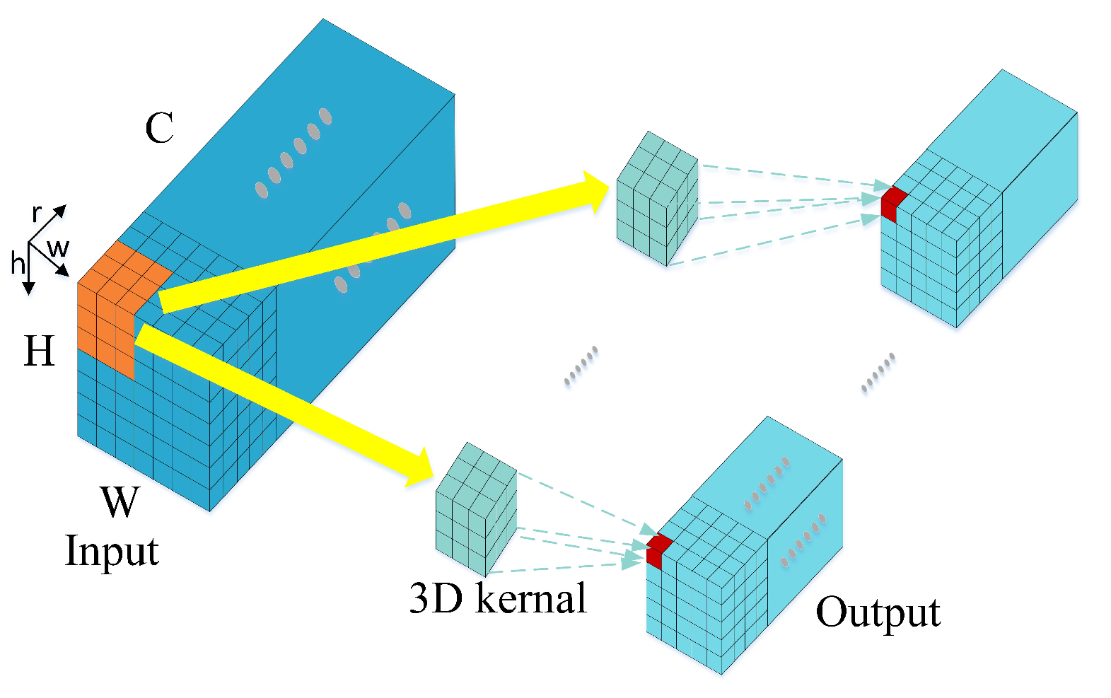
Three-dimensional convolution is an operation that convolves the 3D convolution kernel and 3D data, whose operation process is shown in Figure 1. The input is denoted as , where H is the height, W is the width and C indicates the spectral dimension of the input data. The convolution kernel slides in the input data along the direction of the arrow in Figure 1 and the dot product sum of the 3D convolution kernel and the input data are calculated.
The value v for the j-th feature map at the spatial location in the l-th layer can be given by
where is the number of convolutional kernels in the l-th layer. is the value of the m-th 3D convolution kernel in the j-th layer at the position and is the bias of the l-th layer connected to the j-th 3D feature data. is the activation function.
Activation and batch normalization (BN) [38] operations are performed after the convolution operation of each layer and the result is inputted to the next convolution layer. Since the inter-frame motion information with spatial dimension can be represented well using 3D-CNN, the inter-spectrum correlation with spatial dimension for HSI can be seen as the inter-frame motion information with spatial. Thus, this paper uses 3D-CNN to extract the joint SSFs.
2.2. Attention Mechanism
The attention mechanism can select the information that is more critical to the current target task from a large amount of information and it is broadly used in deep learning tasks such as image recognition and natural language processing [39].
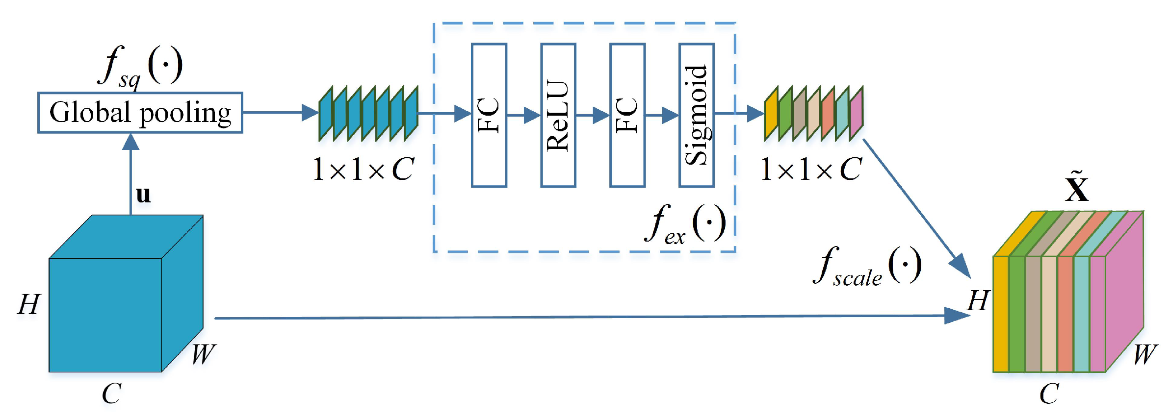
Channel attention enables the network to automatically learn the importance of different feature channels by assigning different weights to each spectral channel. To compensate for the fact that the depth-wise convolution applies a singular filter to every input channel [40], which ignores channel information, a module of depth-wise convolution and channel attention to jointly extract space–spectral information is designed in this paper. This module uses the residual structure to perform identity mapping between the original features and the features after convolution and channel attention processing, which further improves the classification performance of the algorithm. SENet [41] is a representative method for channel attention and its main structure is the SE module, which is shown in Figure 2.
The SE includes three parts: squeeze, excitation and feature recalibration. Specifically, SE mainly consists of a global average pooling (GAP) and two fully connected (FC) layers.
(1) Squeeze
This part adopts GAP. Its operation is to average the original feature map of a spectral band along the spatial dimension. Thus, a real average is obtained for a spectral channel with a global acceptance field to some extent. The formula for the average of channel c is as follows:
where is the compression function and represents the 2D feature map of the c-th channel.
(2) Excitation
The excitation consists of two FC layers. The weight of each feature channel can be calculated by the excitation module, which is used to represent the importance of the feature map channel. The excitation action is shown in detail in Equation (3).
where is the excitation formula, is the squeezed feature map, is the ReLU and is the Sigmoid activation function, which is used after the first and second FC layers, respectively. is the weight between the input and the first connected layer. is the weight between the first and the second FC layer.
(3) Feature recalibration
The principal component features recalibration in the spectral dimension is performed according to the weight of each spectral channel since the weights can represent the correlation between the spectral information and the ground objects. The process is given by
where is the final output of the Res-SEConv module, is the c-th channel weight obtained by the excitation operation and .
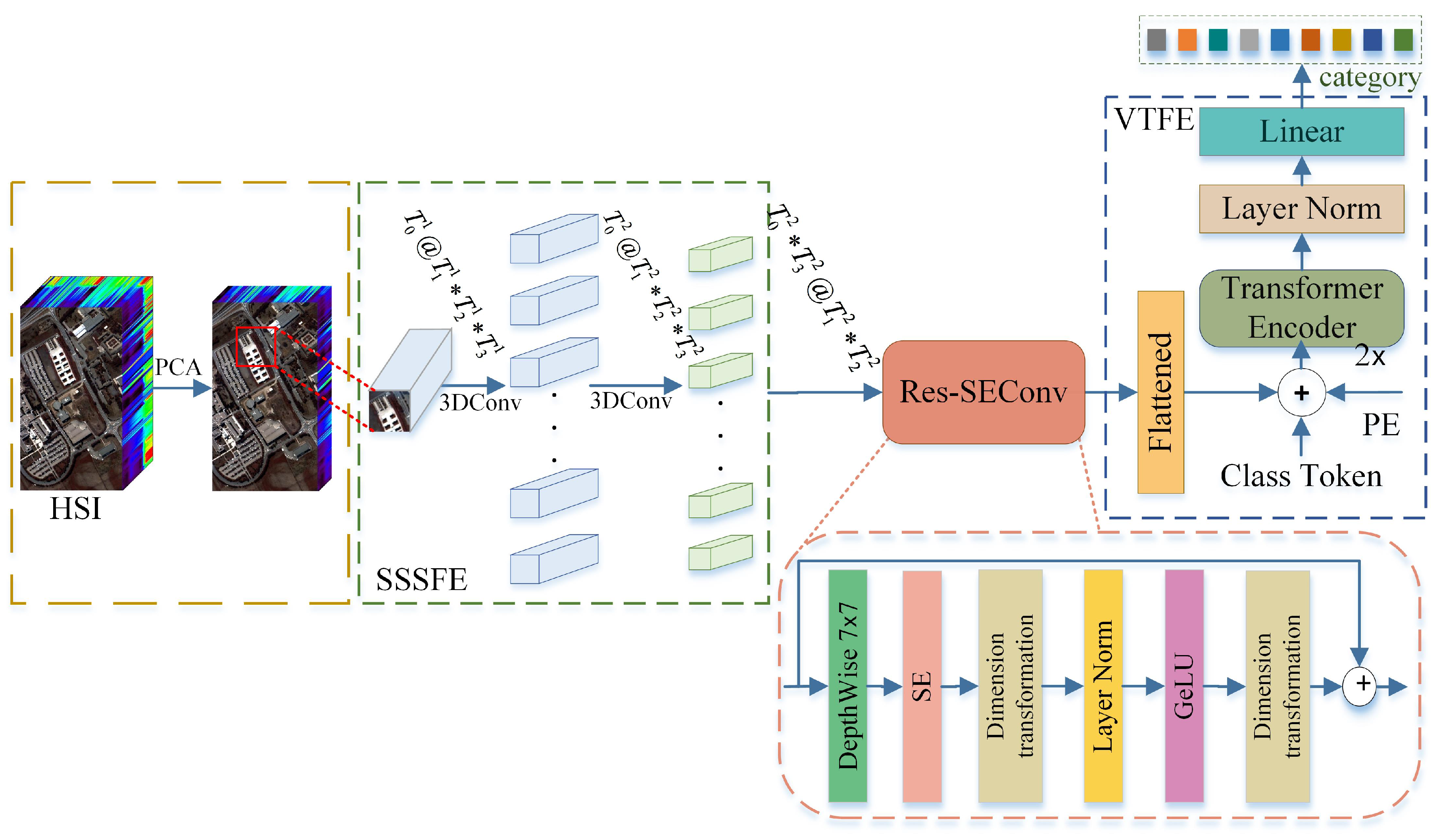
3. Proposed SDFE Method for HSI Classification
To enhance the SSFs from shallow to deep, an end-to-end HSI classification SDFE model (as in Figure 3) is proposed. Firstly, the original hyperspectral HSIs are dimensionally reduced via PCA to retain the spectral components with important contributions. Secondly, the shallow features are extracted via the SSSFE module, which consists of two 3D-CNN layers. Thirdly, the Res-SEConv is designed to strengthen the important channel information. Finally, the VTFE module can further extract SSFs and perform classification. This shallow-to-deep feature extraction method capitalizes on spatial and spectral information at different scales. The approach proposed in this article mainly includes four parts: Band selection, SSSFE module, Res-SEConv module and VTFE module. The specific process is as follows:
3.1. Band Selection
Some bands are not sensitive to ground objects and cannot provide useful ground object information, which results in information redundancy and band noise. Therefore, dimensionality decrease is usually an important pre-processing step in HSI classification.
PCA is a widely used dimensionality reduction algorithm, which aims to find the principal components of the data and uses these principal components to characterize the original data. The raw hyperspectral data are recorded as , where M and N are the width and height of the raw data and L is the spectral band number. After the PCA method, the band number for the original data is reduced from L to B and the obtained data are denoted as . This process only reduces unimportant spectral bands and does not affect spatial information.
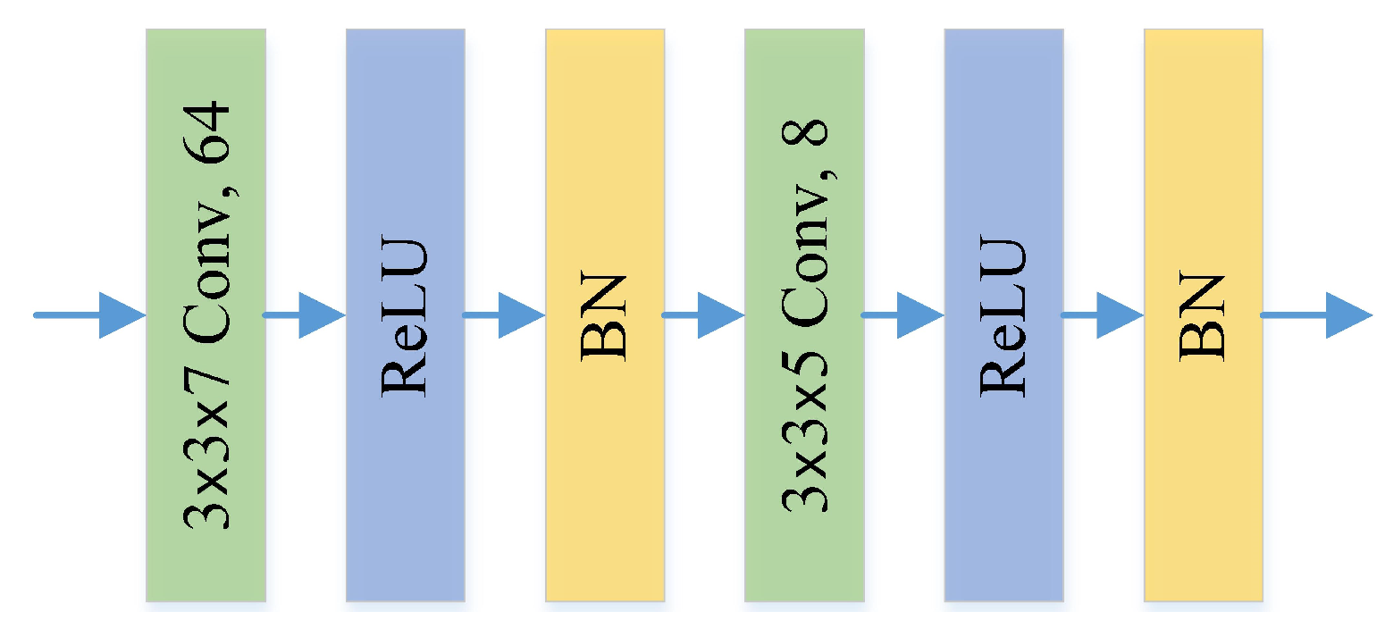
3.2. SSSFE Module
For small training samples, the accuracy will be decreased if the number of layers is increased continually over a certain number. Therefore, to make the most of the high-dimensional features of HSI, an SSSFE module with a two-layer 3D convolution network is designed and a ReLU and BN are performed after each convolutional layer.
To reduce the redundancy of HSI, two different convolution kernels with size and for layers 1 and 2 are set to extract. They not only can reduce the spectral dimension of the input but also effectively reduce the feature redundancy caused by augmenting the number of convolutional layers. The specific details of the SSSFE module are provided in Figure 4.
The image cube is divided into 3D cubes and the size of each cube is , which is the input of the SSSFE module. S is the height and width of the cube and B is the band number of the cube. The ground-truth label of a cube is defined by the center pixel label. Theoretically, the number of 3D convolutional kernels for each 3D convolutional layer is and the size of each kernal is . When the feature block is fed into the 3D convolutional layer, the output dimension becomes . Detailed information concerning the selection of parameters is given in Section 4.3.
3.3. Res-SEConv Module
Compared with ordinary convolution, since a depth-wise convolution kernel can only perform a convolution operation with one channel, the operation parameters are greatly reduced. However, the process of depth-wise convolution does not contain position information and ignores the correlation between channels. Therefore, to enhance the useful spatial and spectral information further and add as few parameters as possible, a Res-SEConv module with depth-wise convolution and channel attention is designed. Its structure (Res-SEConv) is shown in Figure 3. The channel attention adopts SENet [41], which can adaptively obtain correlation for each feature channel. Thus, the important features are enhanced and the unimportant features are weakened according to their correlation.
The process of this module is as follows:
- (1)
- After the SSSFE module, the obtained shallow feature maps are firstly rearranged to obtain feature maps with size . Then, the spatial feature is extracted using the depth-wise convolution module and the channel feature is weighted through the SE module.
- (2)
- The dimension transformation of features is performed after channel attention and the dimension is transformed from to .
- (3)
- Layer Normalization (LN) is first performed on the last dimension. Then, a GeLU activation operation and dimension transformation on the features are carried out. The feature dimension is transformed from to .
- (4)
- The problem of gradient disappearance due to the increasing number of network layers can be solved by the identity mapping of the residual network. Therefore, the skip connection in the Res-SEConv module is designed to prevent overfitting and network degradation.
This module extracts more discriminative space–spectral joint features and only adds a small number of parameters compared to ordinary convolution. The input size of the Res-SEConv module is the same as the output, so it is a plug-and-play module and can be utilized for other computer vision tasks.
3.4. VTFE Module
Although CNN has the features of local connectivity and weight sharing, it is hard to obtain the long-distance spectral correlation. However, the core of HSI analysis is spectral analysis, so we use a ViT to enhance feature maps extracted by the Res-SEConv module. The multi-head attention mechanism of ViT captures the spectral correlation with long-range dependence and maps the global correlations, so it can better represent the spectral features of HSI. The VTFE module consists of the following three parts.
Firstly, the output of the Res-SEConv module is divided into the 2D patches along the spectral dimension and then the 2D patches are mapped to 1D vectors via linear mapping. Secondly, the Position Embedding (PE) is added to each 1D vector. PE can not only preserve the position information of the original 2D block itself before flattening, but can also preserve the relative position information between 2D blocks. Finally, the Class Token for classification is added to the vector with PE. The dimension of the Class Token is the same as that of other tokens and autocorrelation operations are performed between all tokens.
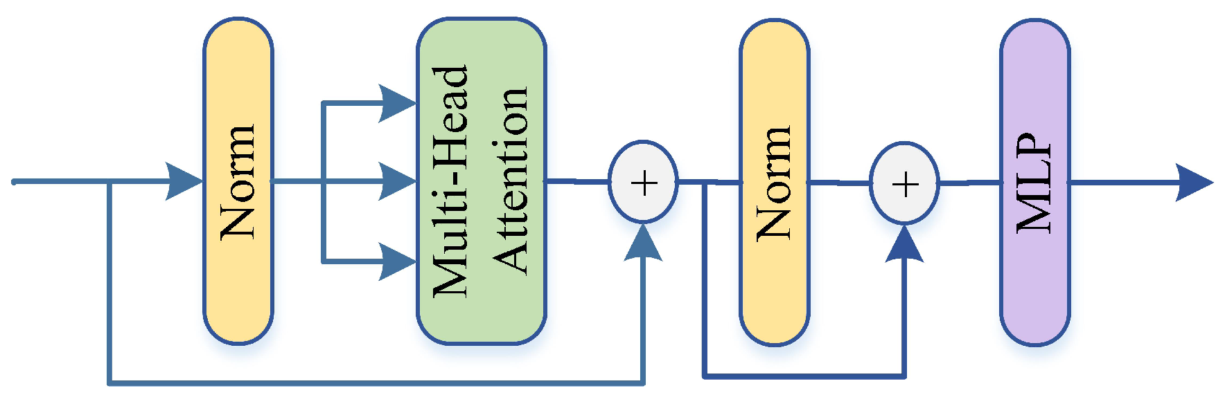
Then, the Transformer Encoder module (as in Figure 5) is the key to the ViT model. The two sub-layers of the LN cascade Multi-head Self-Attention (MSA) and LN cascade MLP layer are alternately connected and the residual connection is used between every two sub-layers.
The attention mechanism of the Transformer can effectively capture the correlation of sequences. Its Self-Attention function essentially maps queries and key-value pairs to the output. Specifically, three learnable weight matrices are defined and the input is linearly changed with the three weight matrices to obtain the matrix of query , key and value . Then, the calculation formula of the output matrix is
where represents the dimension of the input and is also a scale factor. First, the attention score between each and computed in the form of an inner product is scaled by a scaling factor . Then, a softmax operation is performed on the scale scores. Finally, the obtained score is multiplied by the weight of and the output of the attention function is obtained.
The final structure used for the classification is relatively simple, only including an LN and an FC layer. The final classification result can be obtained through the FC layer.
4. Experiments and Results
In this section, the classification performance of the SDFE method and other baselines are analyzed. All experiments in this article have the same experimental environment, in which NVIDIA GeForce RTX3090 GPU, Intel Xeon Gold 6142 [email protected] processor is used and the running memory is 60.9 GB.
The SDFE method adopts the cross-entropy loss function and Adam optimizer, the learning rate is set to 0.0001, the batch size is set to 64, the number of iterations for training on the Indian Pines (IP) dataset is 200 and the number of iterations for training on the Pavia University (PU) and Salinas (SA) datasets is 100.
4.1. Datasets
(1) Indian Pines Dataset
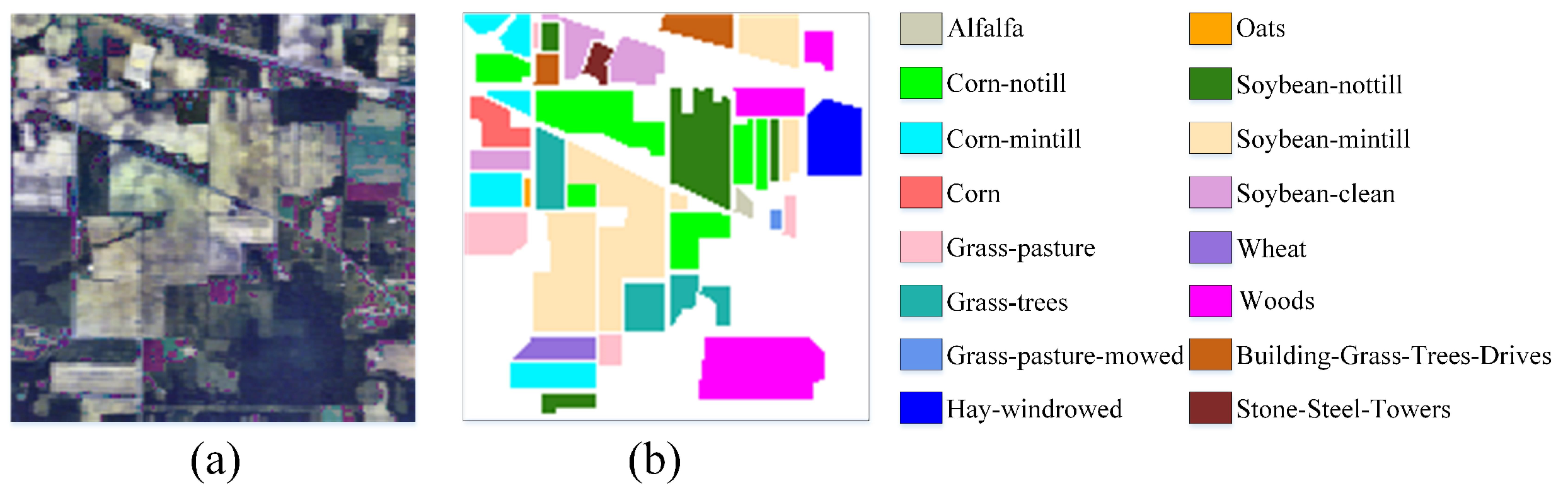
The IP dataset was captured by the AVIRIS imager on an Indian pine tree in the American state of Indiana, which has a spatial resolution of 20 m. There are 16 object categories, 200 bands and 145 × 145 pixels. A total of 10,776 pixels are background and 10,249 pixels are ground objects. Figure 6a is the false-color image and (b) is the ground-truth map.
(2) Pavia University Dataset
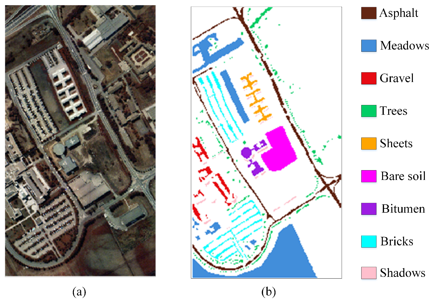
The PU dataset with a resolution of 1.3 m was captured by the ROSIS-03 sensor over the Pavia University in Northern Italy. The number of land cover categories and spectral bands is 9 and 103, respectively. It consists of 610 × 340 pixels and there are only 42,776 ground object pixels. Figure 7a is the false-color image and (b) is the ground-truth map.
(3) Salinas Dataset
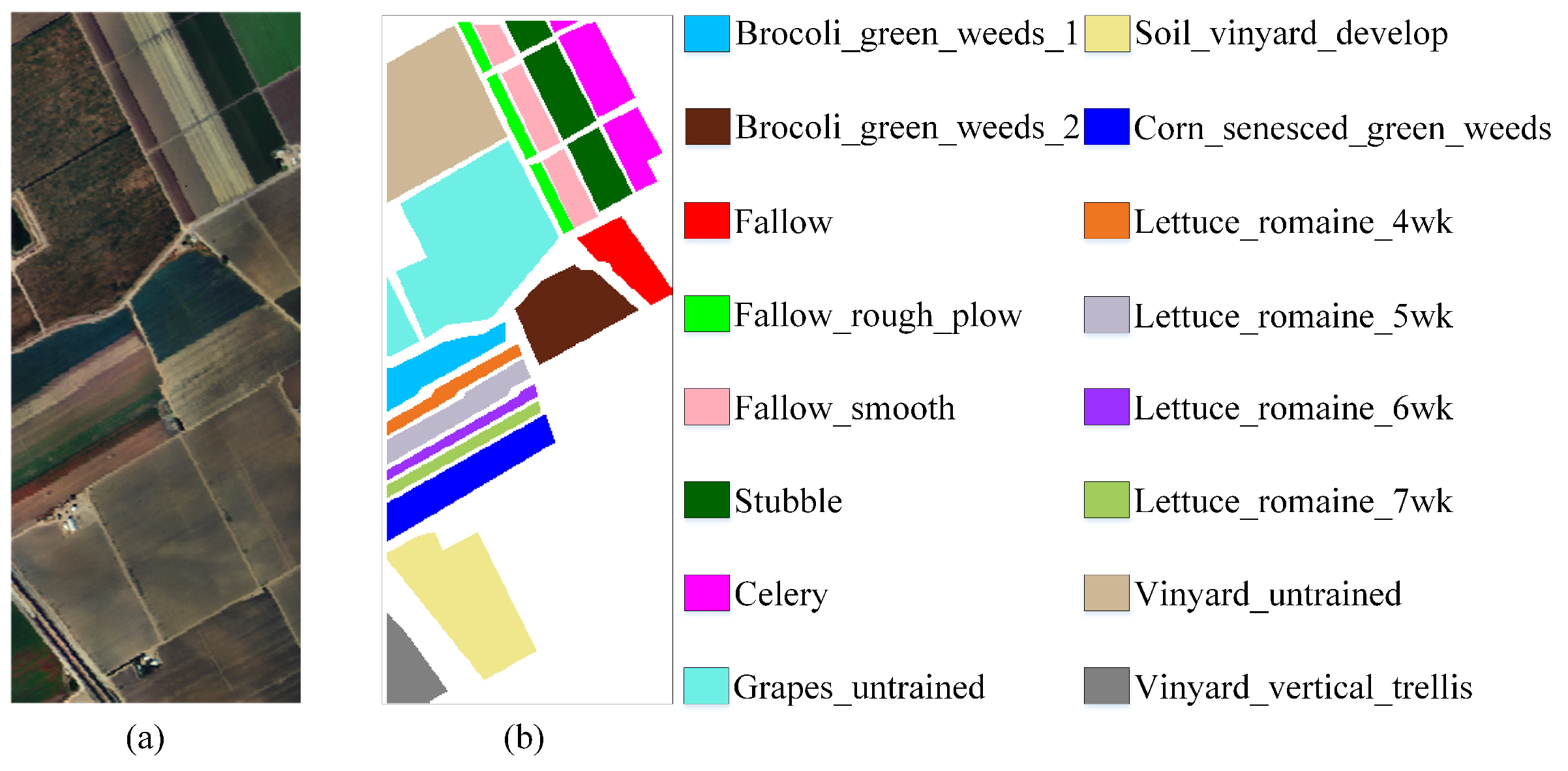
As with the IP dataset, the SA dataset was also captured by the AVIRIS imager. It has a band count of 204 and a spatial resolution of 3.7 m. The dataset contains 512 × 217 pixels and 16 object categories. Among the 111,104 pixels, 54,129 pixels represent the ground objects. Figure 8a is the false-color image and (b) is the ground-truth map.
Table 1 lists the number of training samples, testing samples and land-cover category names for the IP, PU and SA datasets. The training sample number of the IP dataset accounts for 10% of the total and the training sample number of the PU and SA datasets accounts for 5%.
4.2. Evaluation Criterions
The goal of the HSI classification task is to assign a category to each pixel in the image. The assigned categories are compared with the ground truth values. By studying current classification evaluation criteria, the overall accuracy (OA), average accuracy (AA) and Kappa coefficient (Kappa) are selected to evaluate the results of the SDFE method and other methods in this paper. Larger values of these indicators represent better classification effectiveness. OA represents the percentage of correctly classified samples among all test samples, which indicates the correct prediction effect. AA represents the average of the classification accuracies for each category of samples. The Kappa coefficient is a statistical metric that measures the agreement degree between the classification results and ground truth.
OA is formulated by this equation
where is the number of samples that are actually positive and predicted to be positive, is the number of samples that are actually negative and predicted to be negative, is the number of samples that are actually negative but are predicted to be positive and is the number of samples that are actually positive but are predicted to be negative.
AA is formulated by the Equation (7):
where is the of class i, is the of class i and n is the number of categories.
4.3. Model Parameters Selection
In this subsection, we analyze several parameters that have an impact on the classification results, such as the selection of PCA, the input patch size, the 3D convolutional kernel number, the learning rate, batch size and the size of the depth-wise convolutional kernel.
(1) The selection of PCA
HSI contains a lot of redundant and noisy information in the spectral channel. Therefore, it is very challenging to adequately extract spectral information from the images. The comparative experiments using the PCA and LDA preprocessing methods were conducted on the IP dataset and the results are shown in Table 2. It can be seen that the results using PCA are better than those using LDA, so PCA is selected to extract the principal spectra.
The number of the principal components was selected as 20, 30, 50, 100 and 200 for the Indian Pines dataset and 20, 30 and 50 for the Pavia University dataset and Salinas dataset for the experiments. The experimental results on the three datasets are shown in Table 3, Table 4 and Table 5, respectively. It can be found that both the network parameters and the running time increase as the number of the principal components increases, When the principal component number is 30, the optimum classification results can be obtained. Therefore, the principal component number is taken as 30 in this paper. That is, 30 bands of spectra are selected as the HSI spectral features.
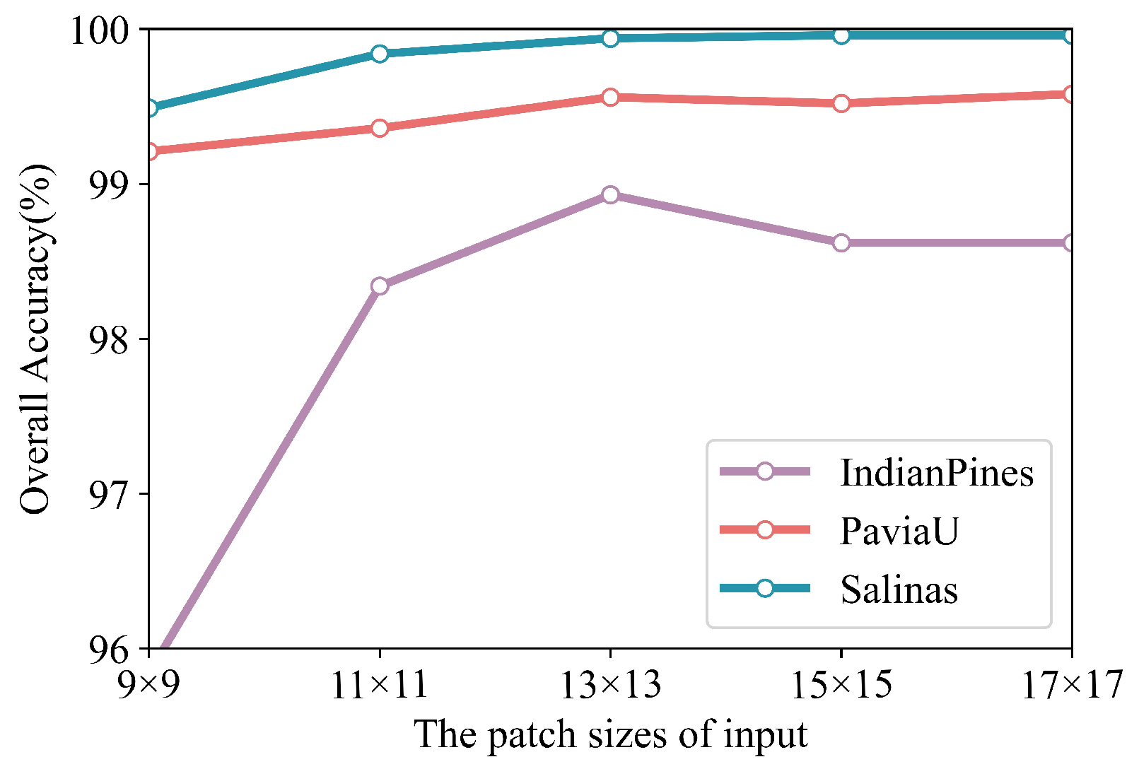
(2) Experiments on the patch size of the input
Different input sizes can affect the classification results of the network, so the selection experiments with different input sizes are carried out. Figure 9 demonstrates the classification metric OA on different patch sizes. We can find that the OA improves with the increase in the input patch and stops improving when the patch reaches . Therefore, the size of the input selected in this paper is .
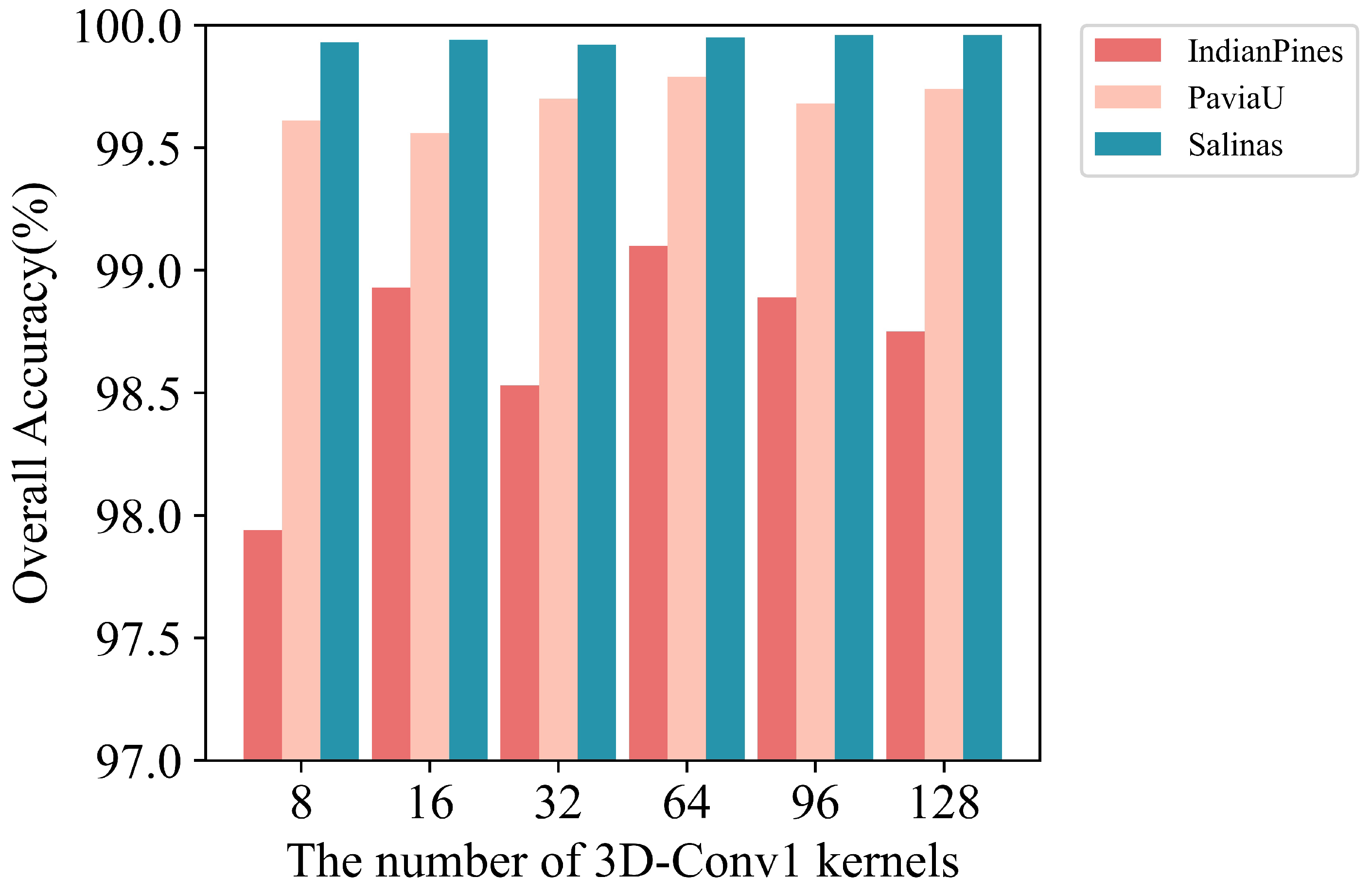
(3) Experiments on the number of 3D convolutional kernels
The number of convolution kernels of the two 3D convolutional layers is denoted as and , respectively. To reduce the amount of data sent to ViT as much as possible, is set to 8. The convolutional kernel number of the 1st layer 3D-CNN is set to 8, 16, 32, 64 and 128 respectively. The overall accuracies are shown in Figure 10. When the convolutional kernel number is 64, the classification accuracies for the three datasets are all the best, so is set to 64 in this paper.
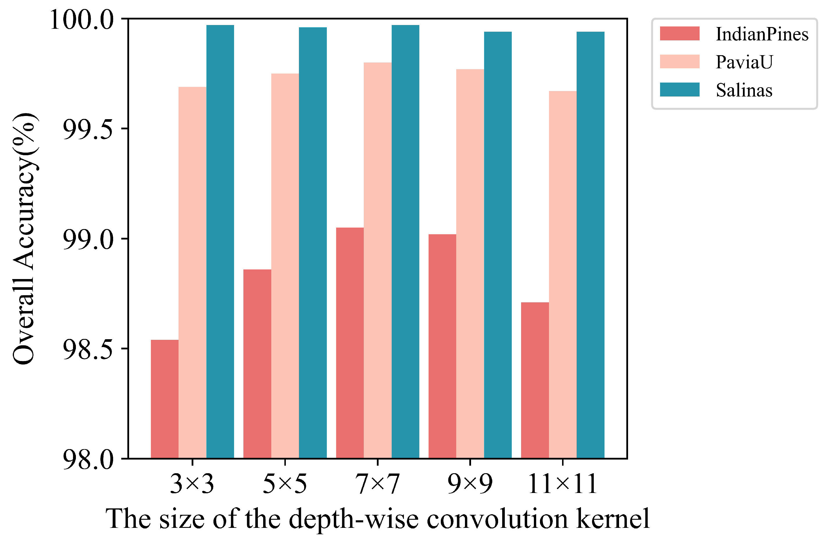
(4) Experiments on the size of the depth-wise convolutional kernels
The depth-wise convolutional kernel size in the Res-SEConv module is set experimentally. The size of the depth-wise convolution kernel is recorded as . For G being 3, 5, 7, 9 and 11, respectively, the classification results are displayed in Figure 11. We can find that the size of the depth-wise convolutional kernel in the Res-SEConv module has the greatest impact on the IP dataset and has less impact on the other two datasets. However, the classification accuracy shows an increasing trend followed by a decreasing trend with an increase in G. The highest OAs are achieved for all three datasets when the kernel size is . Therefore, the depth-wise convolutional kernel size is set to .
(5) Experiments on the activation function of the Res-SEConv module
The activation in the Res-SEConv module is GeLU. Unlike ReLU, GELU weights the inputs according to their magnitude; ReLUs are gated according to the sign of the inputs. GeLU is intuitively more in line with the natural understanding and has been experimentally superior to ReLU in several computer vision tasks. The comparison experiments between ReLu and GeLU in the Res-SEConv module are conducted and the experimental results are shown in Table 6. It can be seen that the general result of using GeLU in the Res-SEConv module is better than using ReLU.
(6) Experiments on the learning rate and batch size
4.4. Ablation Experiments
Five sets of ablation experiments on the SSSFE module, Res-SEConv module and VTFE module are designed (as in Table 9) and the experimental results on the IP dataset further demonstrate the effectiveness of each module in the SDFE method.
From Table 9, we can find that the OA, AA and Kappa are 90.10%, 92.98% and 88.69%, respectively, while using the CNN-based SSSFE module and Res-SEConv module. Compared with it, the OA and Kappa have an increase of about 1%, but AA decreases about 4.74% while only using the VTFE module, which indicates the Transformer is effective in HSI classification. When the SSSFE module is added to the VTFE module, the OA, AA and Kappa are increased by 7.04%, 10.05% and 3.03%, respectively. When the Res-SEConv module is added to the VTFE module, the OA, AA and Kappa are increased by 4.26%, 5.82% and 4.85%, respectively. Overall, the shallow feature extraction using the SSSFE module or Res-SEConv module is superior to no shallow feature extraction before the VTFE module for HSI classification. While the three modules work together, OA, AA and Kappa reach more than 99%, which are the best classification results. This not only proved the effectiveness of the SDFE method but also proved that the constructed SSSFE and Res-SEConv modules can jointly strengthen shallow further.
4.5. Comparison Experiments
To compare the discrepancy between the SDFE method and other baselines, comparative experiments are conducted on the datasets of IP, PU and SA. Representative methods are selected for comparative experiments, which include traditional SVM machine learning method [14], CNN-based methods, such as 2D-CNN [22], 3D-CNN [23], HybridSN [24] and Transformer-based methods ViT [30] and SSFTT [35]. These comparative experiments are described as follows:
- (1)
- 2D-CNN: The network contains two convolutional layers of size with the numbers 30 and 90 and three FC layers. The activation function and classifier are ReLU and SoftMax, respectively.
- (2)
- 3D-CNN: The network contains three convolutional layers and three FC layers.
- (3)
- HybridSN: This contains three 3D convolutional layers and one 2D convolutional layer, as well as three FC layers.
- (4)
- ViT: The input size of the network is . The remaining parameters are the same as those given in [31].
- (5)
- SSFTT: The specific network structure settings are the same as in [35].
The comparisons of the classification performance between SDFE and other baselines on the three datasets are shown in Table 10, Table 11 and Table 12, which proves that the SDFE method can obtain the best classification results.
The accuracies of SDFE are greatly improved compared with other methods for the IP dataset. It significantly outperforms traditional machine learning methods and CNNs and slightly outperforms Transformer-based classification models for the PU and SA datasets. This may be because CNN-based methods lose long-term information to some extent and Transformer-based methods cannot fully extract spatial neighborhood information. However, the SSFTT method and the proposed method make use of the advantages of both CNN and Transformer to some extent. In particular, the shallow spatial and spectrum features are enhanced using the constructed SSSFE module and Res-SEConv module, respectively, which greatly promote the classification effectiveness.
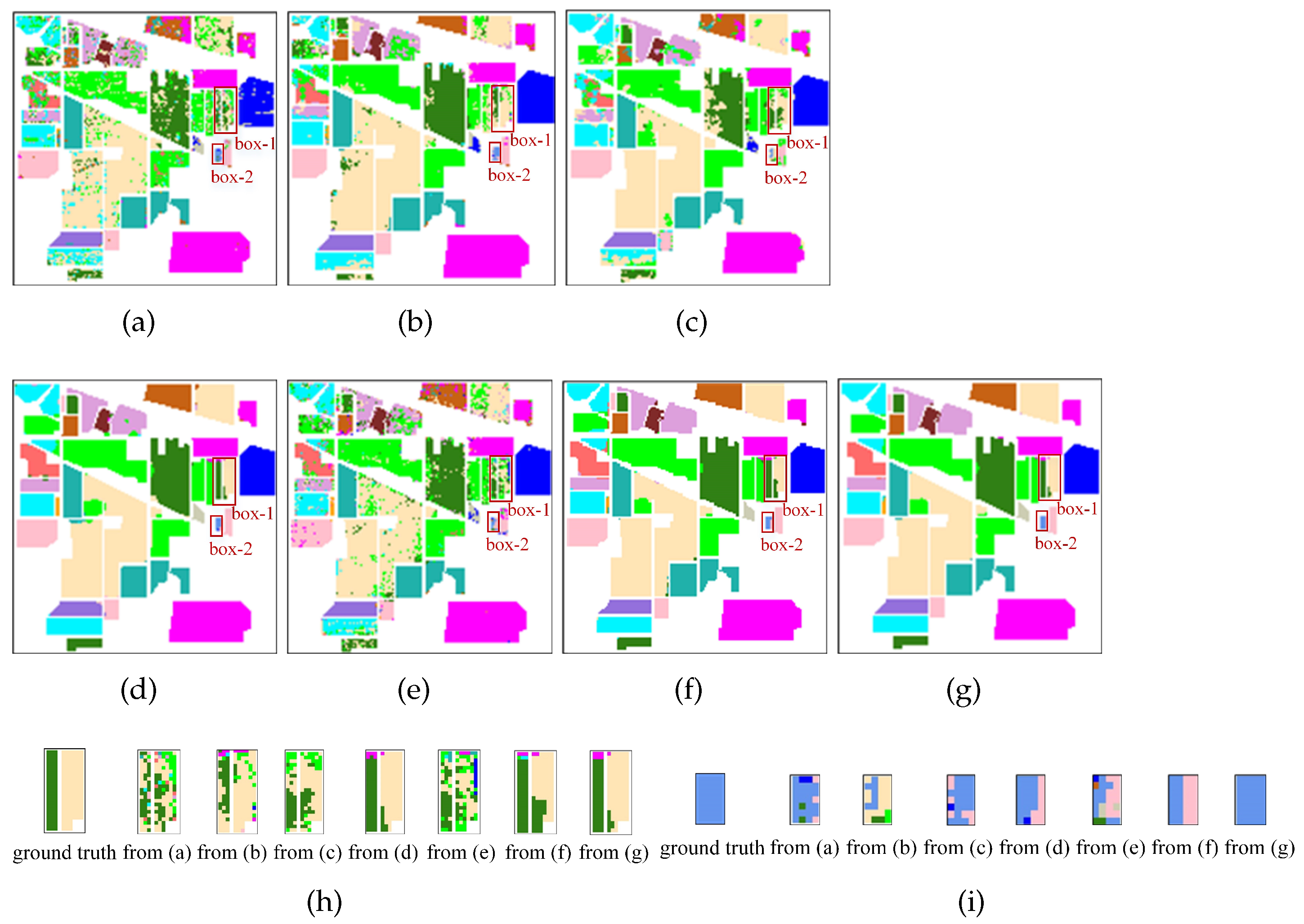
To observe the classification effectiveness, the classification maps using the above methods are given in Figure 12, Figure 13 and Figure 14. For the sake of clear presentation, some illegible misclassification points are framed with red rectangles and are enlarged as shown in Figure 12h,i, Figure 13 and Figure 14h, respectively. The first image is the ground truth and then the remaining images correspond to Figure 12a–g in sequence from left to right for Figure 12h,i and from top to bottom for Figure 13h and Figure 14h. It can be seen that the classification maps obtained by the SDFE network are most similar to the ground truth. SVM, 2D-CNN, HybridSN, 3D-CNN and ViT obviously cannot identify the type accurately and have poor performance.
Figure 12 suggests that the Grass-Pasture-mowed (light blue) marked by the red box-1 in the middle area of the IP dataset is the most difficult to distinguish, which is easily misclassified as the Grass-Pasture (light pink). In addition, the differences between the results are large when using different methods in the areas marked by the red box-2. Compared with using the SSFTT method, the soybean-mintill (dark green) and soybean-nottill (yellow) can be classified better using the SDFE method.
For the PU dataset, the results of the SDFE method for classification are the most prominent in the marked area (Figure 13). The edge misclassification of the Bricks class (light blue) using the other methods is significantly corrected by using the proposed method.
For the SA dataset, the classification maps (Figure 14) demonstrate that the SDFE method is more precise than baselines at the boundaries between the different categories, such as the boundary between the Fallow_rough_plow (pink) and Fallow_smooth (green) marked by a red box. In conclusion, the benefits of the SDFE method are further illustrated.
To investigate the effectiveness of SDFE with different proportions of training data, training samples are randomly selected of 5%, 10%, 15% and 20% of the IP dataset, as well as 2%, 5%, 8% and 11% of the PU and SA datasets. Figure 15 shows the classification accuracies under different training data ratios. It can be found that the classification accuracies of all compared methods show an upward trend as the proportion of training samples increases. The advantage of SDFE is more obvious than baselines under a few training samples, which indicates that SDFE is still useful for fewer samples. However, due to a large amount of computation of the Transformer, the SDFE method has certain limitations on memory consumption and time cost and thus needs to be optimized in future research.
5. Discussion
To evaluate the performance of the proposed SDFE method, we conducted experiments on the training and testing time using 2D-CNN, 3D-CNN, HybridSN, ViT, SSFTT and our method, which are compared as shown in Table 13. It can be seen that the training times of our method on the IP, PU and SA datasets are 239.75 s, 266.09 s and 308.35 s, respectively. It can be seen that the time consumption using the proposed SDFE method is relatively large, but the classification results are the best.
The memory consumptions are shown in Table 14, which includes the total params, the params sizes and Flops. Table 14 suggests that the SDFE method has fewer number parameters but higher Flops. Therefore, the network lightweight will be considered in future work. On the one hand, the number of the training samples can be reduced by the sample augmentation methods, such as some time-frequency analysis and active learning methods. On the other hand, the structure of Transformer can be optimized for the purpose of reducing memory and time consumption.
6. Conclusions
To completely exploit the joint SSFs of shallow and deep scales, we propose an HSI classification framework SDFE based on CNN and Transformer. In SDFE, an SSSFE module (two-layer 3D-CNN) is constructed for shallow SSF extraction first. Then, the spectral features are weighted according to their correlations with the ground objects using a Res-SEConv module. Lastly, the VTFE module is used for extracting deep SSFs and completing the classification. The experiments based on three benchmark datasets indicate that the SDFE method is superior to other models in terms of classification effectiveness. Although SDFE has made good progress in classification results, it is time-consuming for the model training. Therefore, our upcoming work is to improve the network structure and construct a lightweight network.
Author Contributions
Conceptualization, L.Z.; Data curation, X.M.; Formal analysis, S.H.; Funding acquisition, L.Z. and S.H.; Investigation, L.Z. and X.W.; Methodology, L.Z.; Project administration, L.Z.; Resources, Y.Y.; Software, X.M.; Supervision, L.Z. and K.Z.; Validation, X.M. and X.W.; Visualization, X.M.; Writing–original draft, X.M.; Writing–review & editing, L.Z. and K.Z. All authors have read and agreed to the published version of the manuscript.
Funding
This work was partially funded by the National Natural Science Foundation of China (No. 62171247, 41921781) and the Natural Foundation of Shandong Province (ZR2016FQ14).
Data Availability Statement
The datasets presented in this paper can be obtained through https://www.ehu.eus/ccwintco/index.php/Hyperspectral_Remote_Sensing_Scenes accessed on 11 December 2022.
Acknowledgments
We would like to appreciate the National Natural Science Foundation of China and the Natural Foundation of Shandong Province for supporting our work.
Conflicts of Interest
The authors declare no conflict of interest.
Abbreviations
The following abbreviations are used in this manuscript:
| HSI | Hyperspectral Image |
| SDFE | Shallow-to-Deep Feature Enhancement |
| CNN | Convolutional Neural Networks |
| ViT | Vision-Transformer |
| LDA | Linear Discriminant Analysis |
| PCA | Principal Component Analysis |
| SSSFE | Shallow Spatial–Spectral Feature Extraction |
| SSF | Spatial–Spectral Features |
| IP | Indian Pines |
| PU | Pavia University |
| SA | Salinas |
| BN | Batch Normalization |
| GAP | Global Average Pooling |
| FC | Fully Connected |
| PE | Position Embedding |
| MSA | Multi-head Self-Attention |
| LN | Layer Normalization |
| OA | Overall Accuracy |
| AA | Average Accuracy |
| Kappa | Kappa coefficient |
References
- Wang, J.; Zhang, L.; Tong, Q.; Sun, X. The Spectral Crust project—Research on new mineral exploration technology. In Proceedings of the 2012 IEEE 4th Workshop on Hyperspectral Image and Signal Processing: Evolution in Remote Sensing (WHISPERS), Shanghai, China, 4–7 June 2012; pp. 1–4. [Google Scholar]
- Bioucas-Dias, J.M.; Plaza, A.; Camps-Valls, G.; Scheunders, P.; Nasrabadi, N.; Chanussot, J. Hyperspectral remote sensing data analysis and future challenges. IEEE Geosci. Remote Sens. Mag. 2013, 1, 6–36. [Google Scholar] [CrossRef] [Green Version]
- Uzkent, B.; Rangnekar, A.; Hoffman, M. Aerial vehicle tracking by adaptive fusion of hyperspectral likelihood maps. In Proceedings of the IEEE Conference on Computer Vision and Pattern Recognition Workshops, Honolulu, HI, USA, 21–26 July 2017; pp. 39–48. [Google Scholar]
- Ardouin, J.P.; Lévesque, J.; Rea, T.A. A demonstration of hyperspectral image exploitation for military applications. In Proceedings of the IEEE 2007 10th International Conference on Information Fusion, Quebec, QC, Canada, 9–12 July 2007; pp. 1–8. [Google Scholar]
- Vaishnavi, B.B.S.; Pamidighantam, A.; Hema, A.; Syam, V.R. Hyperspectral Image Classification for Agricultural Applications. In Proceedings of the 2022 IEEE International Conference on Electronics and Renewable Systems (ICEARS), Tuticorin, India, 16–18 March 2022; pp. 1–7. [Google Scholar]
- Schimleck, L.; Ma, T.; Inagaki, T.; Tsuchikawa, S. Review of near infrared hyperspectral imaging applications related to wood and wood products. Appl. Spectrosc. Rev. 2022, 57, 2098759. [Google Scholar] [CrossRef]
- Liao, X.; Liao, G.; Xiao, L. Rapeseed Storage Quality Detection Using Hyperspectral Image Technology—An Application for Future Smart Cities. J. Test. Eval. 2022, 51, JTE20220073. [Google Scholar] [CrossRef]
- Jaiswal, G.; Sharma, A.; Yadav, S.K. Critical insights into modern hyperspectral image applications through deep learning. Wiley Interdiscip. Rev. Data Min. Knowl. Discov. 2021, 11, e1426. [Google Scholar] [CrossRef]
- Hyperspectral Remote Sensing Scenes. Available online: https://www.ehu.eus/ccwintco/index.php/Hyperspectral_Remote_Sensing_Scenes (accessed on 11 December 2022).
- Bandos, T.V.; Bruzzone, L.; Camps-Valls, G. Classification of hyperspectral images with regularized linear discriminant analysis. IEEE Trans. Geosci. Remote Sens. 2009, 47, 862–873. [Google Scholar] [CrossRef]
- Villa, A.; Benediktsson, J.A.; Chanussot, J.; Jutten, C. Hyperspectral image classification with independent component discriminant analysis. IEEE Trans. Geosci. Remote Sens. 2011, 49, 4865–4876. [Google Scholar] [CrossRef] [Green Version]
- Licciardi, G.; Marpu, P.R.; Chanussot, J.; Benediktsson, J.A. Linear versus nonlinear PCA for the classification of hyperspectral data based on the extended morphological profiles. IEEE Geosci. Remote Sens. Lett. 2011, 9, 447–451. [Google Scholar] [CrossRef] [Green Version]
- Zhou, L.; Xu, E.; Hao, S.; Ye, Y.; Zhao, K. Data-Wise Spatial Regional Consistency Re-Enhancement for Hyperspectral Image Classification. Remote Sens. 2022, 14, 2227. [Google Scholar] [CrossRef]
- Mitchell, T.M. Machine Learning; McGraw-Hill: New York, NY, USA, 1997; Volume 1, p. 9. [Google Scholar]
- Li, J.; Bioucas-Dias, J.M.; Plaza, A. Semisupervised hyperspectral image segmentation using multinomial logistic regression with active learning. IEEE Trans. Geosci. Remote Sens. 2010, 48, 4085–4098. [Google Scholar] [CrossRef] [Green Version]
- Tipping, M.E. Sparse Bayesian learning and the relevance vector machine. J. Mach. Learn. Res. 2001, 1, 211–244. [Google Scholar]
- Melgani, F.; Bruzzone, L. Classification of hyperspectral remote sensing images with support vector machines. IEEE Trans. Geosci. Remote Sens. 2004, 42, 1778–1790. [Google Scholar] [CrossRef]
- Ghamisi, P.; Maggiori, E.; Li, S.; Souza, R.; Tarablaka, Y.; Moser, G.; De Giorgi, A.; Fang, L.; Chen, Y.; Chi, M.; et al. New frontiers in spectral–spatial hyperspectral image classification: The latest advances based on mathematical morphology, Markov random fields, segmentation, sparse representation and deep learning. IEEE Geosci. Remote Sens. Mag. 2018, 6, 10–43. [Google Scholar] [CrossRef]
- Kang, X.; Li, S.; Benediktsson, J.A. Spectral–spatial hyperspectral image classification with edge-preserving filtering. IEEE Trans. Geosci. Remote Sens. 2013, 52, 2666–2677. [Google Scholar] [CrossRef]
- Ma, K.Y.; Chang, C.I. Iterative Training Sampling Coupled with Active Learning for Semisupervised Spectral–Spatial Hyperspectral Image Classification. IEEE Trans. Geosci. Remote. Sens. 2021, 59, 8672–8692. [Google Scholar] [CrossRef]
- Audebert, N.; Le Saux, B.; Lefèvre, S. Deep learning for classification of hyperspectral data: A comparative review. IEEE Geosci. Remote Sens. Mag. 2019, 7, 159–173. [Google Scholar] [CrossRef] [Green Version]
- Makantasis, K.; Karantzalos, K.; Doulamis, A.; Doulamis, N. Deep supervised learning for hyperspectral data classification through convolutional neural networks. In Proceedings of the 2015 IEEE International Geoscience and Remote Sensing Symposium (IGARSS), Milan, Italy, 26–31 July 2015; pp. 4959–4962. [Google Scholar]
- Hamida, A.B.; Benoit, A.; Lambert, P.; Amar, C.B. 3-D deep learning approach for remote sensing image classification. IEEE Trans. Geosci. Remote Sens. 2018, 56, 4420–4434. [Google Scholar] [CrossRef] [Green Version]
- Roy, S.K.; Krishna, G.; Dubey, S.R.; Chaudhuri, B.B. HybridSN: Exploring 3-D–2-D CNN feature hierarchy for hyperspectral image classification. IEEE Geosci. Remote Sens. Lett. 2019, 17, 277–281. [Google Scholar] [CrossRef] [Green Version]
- Cao, J.; Chen, Z.; Wang, B. Deep convolutional networks with superpixel segmentation for hyperspectral image classification. In Proceedings of the 2016 IEEE International Geoscience and Remote Sensing Symposium (IGARSS), Beijing, China, 10–15 July 2016; pp. 3310–3313. [Google Scholar]
- He, K.; Zhang, X.; Ren, S.; Sun, J. Deep residual learning for image recognition. In Proceedings of the IEEE Conference on Computer Vision and Pattern Recognition, Las Vegas, NV, USA, 27–30 June 2016; pp. 770–778. [Google Scholar]
- Zhong, Z.; Li, J.; Luo, Z.; Chapman, M. Spectral–spatial residual network for hyperspectral image classification: A 3-D deep learning framework. IEEE Trans. Geosci. Remote Sens. 2017, 56, 847–858. [Google Scholar] [CrossRef]
- Chang, Y.L.; Tan, T.H.; Lee, W.H.; Chang, L.; Chen, Y.N.; Fan, K.C.; Alkhaleefah, M. Consolidated Convolutional Neural Network for Hyperspectral Image Classification. Remote Sens. 2022, 14, 1571. [Google Scholar] [CrossRef]
- Yue, J.; Fang, L.; He, M. Spectral–spatial latent reconstruction for open-set hyperspectral image classification. IEEE Trans. Image Process. 2022, 31, 5227–5241. [Google Scholar] [CrossRef]
- Vaswani, A.; Shazeer, N.; Parmar, N.; Uszkoreit, J.; Jones, L.; Gomez, A.N.; Kaiser, Ł.; Polosukhin, I. Attention is all you need. Adv. Neural Inf. Process. Syst. arXiv 2017, arXiv:1706.03762. [Google Scholar]
- Dosovitskiy, A.; Beyer, L.; Kolesnikov, A.; Weissenborn, D.; Zhai, X.; Unterthiner, T.; Dehghani, M.; Minderer, M.; Heigold, G.; Gelly, S.; et al. An image is worth 16x16 words: Transformers for image recognition at scale. arXiv 2020, arXiv:2010.11929. [Google Scholar]
- Hong, D.; Han, Z.; Yao, J.; Gao, L.; Zhang, B.; Plaza, A.; Chanussot, J. SpectralFormer: Rethinking hyperspectral image classification with transformers. IEEE Trans. Geosci. Remote Sens. 2021, 59, 5518615. [Google Scholar] [CrossRef]
- He, X.; Chen, Y.; Lin, Z. Spatial–spectral transformer for hyperspectral image classification. Remote Sens. 2021, 13, 498. [Google Scholar] [CrossRef]
- Zhong, Z.; Li, Y.; Ma, L.; Li, J.; Zheng, W.S. Spectral–spatial transformer network for hyperspectral image classification: A factorized architecture search framework. IEEE Trans. Geosci. Remote Sens. 2021, 59, 5514715. [Google Scholar] [CrossRef]
- Sun, L.; Zhao, G.; Zheng, Y.; Wu, Z. Spectral–Spatial Feature Tokenization Transformer for Hyperspectral Image Classification. IEEE Trans. Geosci. Remote Sens. 2022, 60, 5522214. [Google Scholar] [CrossRef]
- Yang, K.; Sun, H.; Zou, C.; Lu, X. Cross-Attention Spectral–Spatial Network for Hyperspectral Image Classification. IEEE Trans. Geosci. Remote Sens. 2022, 60, 5518714. [Google Scholar] [CrossRef]
- Han, G. A Multibranch Crossover Feature Attention Network for Hyperspectral Image Classification. Remote Sens. 2022, 14, 5778. [Google Scholar]
- Ioffe, S.; Szegedy, C. Batch normalization: Accelerating deep network training by reducing internal covariate shift. In Proceedings of the International Conference on Machine Learning. PMLR, Lille, France, 6–11 July 2015; pp. 448–456. [Google Scholar]
- Hommel, B.; Chapman, C.S.; Cisek, P.; Neyedli, H.F.; Song, J.H.; Welsh, T.N. No one knows what attention is. Atten. Percept. Psychophys. 2019, 81, 2288–2303. [Google Scholar] [CrossRef]
- Howard, A.G.; Zhu, M.; Chen, B.; Kalenichenko, D.; Wang, W.; Weyand, T.; Andreetto, M.; Adam, H. Mobilenets: Efficient convolutional neural networks for mobile vision applications. arXiv 2017, arXiv:1704.04861. [Google Scholar]
- Hu, J.; Shen, L.; Sun, G. Squeeze-and-excitation networks. In Proceedings of the IEEE Conference on Computer Vision and Pattern Recognition, Salt Lake City, UT, USA, 18–23 June 2018; pp. 7132–7141. [Google Scholar]
Figure 1.
The process of 3D convolution.

Figure 2.
The SE module.

Figure 3.
The classification structure of SDFE.

Figure 4.
The SSSFE module.

Figure 5.
The Transformer Encoder.

Figure 6.
The IP dataset. (a) False-color image. (b) Ground-truth map.

Figure 7.
The PU dataset. (a) False-color image. (b) Ground-truth map.

Figure 8.
The SA dataset. (a) False-color image. (b) Ground-truth map.

Figure 9.
The OAs for three datasets with different patch sizes.

Figure 10.
The OAs for the three datasets with the different 3D convolution kernel numbers.

Figure 11.
The OAs for the three datasets with different depth-wise convolution kernel sizes in the Res-SEConv module.
Figure 11.
The OAs for the three datasets with different depth-wise convolution kernel sizes in the Res-SEConv module.

Figure 12.
The classification maps of the IP dataset. (a) SVM. (b) 2D-CNN. (c) 3D-CNN. (d) HybridSN. (e) ViT. (f) SSFTT. (g) SDFE. (h) The enlarged images of box-1. (i) The enlarged images of box-2.
Figure 12.
The classification maps of the IP dataset. (a) SVM. (b) 2D-CNN. (c) 3D-CNN. (d) HybridSN. (e) ViT. (f) SSFTT. (g) SDFE. (h) The enlarged images of box-1. (i) The enlarged images of box-2.

Figure 13.
The classification maps of the PU dataset. (a) SVM. (b) 2D-CNN. (c) 3D-CNN. (d) HybridSN. (e) ViT. (f) SSFTT. (g) SDFE. (h) The enlarged image.
Figure 13.
The classification maps of the PU dataset. (a) SVM. (b) 2D-CNN. (c) 3D-CNN. (d) HybridSN. (e) ViT. (f) SSFTT. (g) SDFE. (h) The enlarged image.

Figure 14.
The classification maps of the IP dataset. (a) SVM. (b) 2D-CNN. (c) 3D-CNN. (d) HybridSN. (e) ViT. (f) SSFTT. (g) SDFE. (h) The enlarged image.
Figure 14.
The classification maps of the IP dataset. (a) SVM. (b) 2D-CNN. (c) 3D-CNN. (d) HybridSN. (e) ViT. (f) SSFTT. (g) SDFE. (h) The enlarged image.

Figure 15.
The OAs of the SDFE method and other baselines at different training sample percentages. (a) IP dataset. (b) PU dataset. (c) SA dataset.
Figure 15.
The OAs of the SDFE method and other baselines at different training sample percentages. (a) IP dataset. (b) PU dataset. (c) SA dataset.


Table 1.
The number of training and testing samples of each category for the IP, PU and SA datasets.
Table 1.
The number of training and testing samples of each category for the IP, PU and SA datasets.
| IP | PU | SA | |||||||
|---|---|---|---|---|---|---|---|---|---|
| No | Class Name | Train | Test | Class Name | Train | Test | Class Name | Train | Test |
| 1 | Alfalfa | 4 | 42 | Asphalt | 331 | 6300 | Brocoli_green_weeds_1 | 100 | 1909 |
| 2 | Corn-notill | 142 | 1286 | Meadows | 932 | 17,717 | Brocoli_green_weeds_2 | 186 | 3540 |
| 3 | Corn-mintill | 82 | 748 | Gravel | 104 | 1995 | Fallow | 98 | 1878 |
| 4 | Corn | 23 | 214 | Trees | 153 | 2911 | Fallow_rough_plow | 69 | 1325 |
| 5 | Grass-pasture | 48 | 435 | Sheets | 67 | 1278 | Fallow_smooth | 133 | 2545 |
| 6 | Grass-trees | 72 | 658 | Bare soil | 251 | 4778 | Stubble | 197 | 3762 |
| 7 | Grass-pasture-mowed | 3 | 25 | Bitumen | 66 | 1264 | Celery | 178 | 3401 |
| 8 | Hay-windrowed | 47 | 431 | Bricks | 184 | 3498 | Grapes_untrained | 563 | 10,708 |
| 9 | Oats | 2 | 18 | Shadows | 47 | 900 | Soil_vinyard_develop | 310 | 5893 |
| 10 | Soybean-nottill | 97 | 875 | Corn_senesced weeds | 163 | 3115 | |||
| 11 | Soybean-mintill | 245 | 2210 | Lettuce_romaine_4wk | 53 | 1015 | |||
| 12 | Soybean-clean | 59 | 534 | Lettuce_romaine_5wk | 96 | 1831 | |||
| 13 | Wheat | 20 | 185 | Lettuce_romaine_6wk | 45 | 871 | |||
| 14 | Woods | 126 | 1139 | Lettuce_romaine_7wk | 53 | 1017 | |||
| 15 | Building-Grass-Trees | 38 | 348 | Vinyard_untrained | 363 | 6905 | |||
| 16 | Stone-Steel-Towers | 9 | 84 | Vinyard_vertical_trellis | 90 | 1717 | |||
| # | Total | 1017 | 9232 | Total | 2135 | 40,641 | Total | 2697 | 51,432 |
Table 2.
Classification results using PCA and LDA on the IP dataset.
| OA (%) | AA (%) | Kappa (×100) | |
|---|---|---|---|
| PCA | 99.16 | 99.07 | 99.04 |
| LDA | 98.72 | 98.83 | 98.54 |
Table 3.
Experimental results with different PCA coefficients on the IP dataset.
| PCA | OA (%) | AA (%) | Kappa (×100) | Time (s) | Params (M) |
|---|---|---|---|---|---|
| 20 | 98.25 | 98.53 | 98.00 | 236.18 | 4.58 |
| 30 | 99.16 | 99.07 | 99.04 | 239.75 | 6.85 |
| 50 | 98.88 | 99.18 | 98.72 | 240.31 | 11.41 |
| 100 | 98.97 | 99.02 | 98.82 | 272.88 | 22.91 |
| 200 | 98.97 | 99.06 | 98.82 | 420.10 | 46.38 |
Table 4.
Experimental results with different PCA coefficients on the PU dataset.
| PCA | OA (%) | AA (%) | Kappa(×100) | Train Time | Params (M) |
|---|---|---|---|---|---|
| 20 | 99.70 | 99.55 | 99.60 | 233.05 | 4.57 |
| 30 | 99.80 | 99.70 | 99.74 | 266.09 | 6.84 |
| 50 | 99.68 | 99.55 | 99.58 | 271.89 | 11.40 |
Table 5.
Experimental results with different PCA coefficients on the SA dataset.
| PCA | OA (%) | AA (%) | Kappa | Train Time | Params (M) |
|---|---|---|---|---|---|
| 20 | 99.95 | 99.73 | 99.94 | 306.29 | 4.58 |
| 30 | 99.97 | 99.80 | 99.97 | 308.35 | 6.85 |
| 50 | 99.95 | 99.94 | 99.94 | 310.90 | 11.41 |
Table 6.
Comparison results using ReLU and GeLU in Res-SEConv module on the IP dataset.
| OA (%) | AA (%) | Kappa (×100) | |
|---|---|---|---|
| ReLU | 98.86 | 99.07 | 98.70 |
| GeLU | 99.16 | 99.07 | 99.04 |
Table 7.
Comparison experiments with different learning rates on the IP dataset.
| Learning Rate | OA (%) | AA (%) | Kappa (×100) |
|---|---|---|---|
| 0.01 | 98.40 | 98.58 | 98.13 |
| 0.001 | 98.85 | 98.96 | 98.69 |
| 0.0001 | 99.16 | 99.07 | 99.04 |
| 0.00001 | 98.78 | 98.87 | 98.61 |
Table 8.
Comparison experiments with different batch sizes on the IP dataset.
| Batch Size | OA (%) | AA (%) | Kappa (×100) |
|---|---|---|---|
| 32 | 98.90 | 98.88 | 98.13 |
| 64 | 99.16 | 99.07 | 98.69 |
| 128 | 98.49 | 98.98 | 99.04 |
Table 9.
The classification results of ablation experiments on the IP dataset.
| Components | Indicators | ||||
|---|---|---|---|---|---|
| SSSFE | Res-SEConv | VTFE | OA (%) | AA (%) | Kappa (×100) |
| √ | √ | - | 90.10 | 92.98 | 88.69 |
| - | - | √ | 91.66 | 88.24 | 90.50 |
| - | √ | √ | 95.92 | 94.06 | 95.35 |
| √ | - | √ | 98.57 | 98.29 | 98.38 |
| √ | √ | √ | 99.16 | 99.07 | 99.04 |
Table 10.
The classification results (in percent) using SDFE and other baselines for the IP dataset.
Table 10.
The classification results (in percent) using SDFE and other baselines for the IP dataset.
| Class | SVM | 2D-CNN | 3D-CNN | HybridSN | ViT | SSFTT | SDFE (Proposed) |
|---|---|---|---|---|---|---|---|
| 1 | 68.29 | 34.15 | 19.52 | 100.00 | 65.85 | 100.00 | 100.00 |
| 2 | 69.73 | 75.18 | 90.89 | 97.82 | 65.84 | 97.43 | 97.85 |
| 3 | 61.58 | 79.79 | 71.89 | 95.45 | 75.1 | 95.45 | 99.22 |
| 4 | 51.64 | 48.83 | 35.21 | 96.71 | 71.36 | 98.59 | 98.97 |
| 5 | 89.66 | 95.40 | 85.98 | 99.54 | 88.05 | 100.00 | 98.46 |
| 6 | 97.41 | 98.17 | 98.33 | 99.85 | 97.41 | 100.00 | 99.16 |
| 7 | 72.00 | 68.00 | 16.00 | 60.00 | 64.00 | 52.00 | 100.00 |
| 8 | 91.86 | 100.00 | 99.30 | 100.00 | 96.51 | 100.00 | 100.00 |
| 9 | 22.22 | 50.00 | 0.00 | 100.00 | 66.67 | 72.22 | 100.00 |
| 10 | 71.66 | 82.97 | 71.66 | 96.46 | 75.89 | 98.51 | 99.24 |
| 11 | 81.36 | 90.95 | 94.75 | 97.33 | 89.28 | 97.51 | 99.85 |
| 12 | 64.04 | 57.87 | 75.66 | 96.07 | 63.67 | 97.19 | 99.78 |
| 13 | 95.68 | 99.46 | 98.38 | 97.30 | 98.38 | 100.00 | 100.00 |
| 14 | 96.40 | 97.72 | 96.22 | 99.21 | 89.29 | 99.65 | 98.93 |
| 15 | 54.18 | 90.49 | 64.55 | 100.00 | 80.98 | 99.42 | 100.00 |
| 16 | 84.52 | 84.52 | 73.81 | 79.76 | 88.10 | 96.43 | 93.67 |
| OA | 78.50 | 85.89 | 85.88 | 97.57 | 82.2 | 98.06 | 99.16 |
| AA | 73.26 | 78.34 | 68.23 | 94.72 | 79.77 | 94.03 | 99.07 |
| Kappa | 75.37 | 83.80 | 83.68 | 97.23 | 79.61 | 97.79 | 99.04 |
Table 11.
The classification results (in percent) using SDFE and other baselines for the PU dataset.
Table 11.
The classification results (in percent) using SDFE and other baselines for the PU dataset.
| Class | SVM | 2D-CNN | 3D-CNN | HybridSN | ViT | SSFTT | SDFE (Proposed) |
|---|---|---|---|---|---|---|---|
| 1 | 93.33 | 95.51 | 97.71 | 99.63 | 96.84 | 99.98 | 99.90 |
| 2 | 97.83 | 99.68 | 99.90 | 99.87 | 98.59 | 100.00 | 99.92 |
| 3 | 74.42 | 85.66 | 84.95 | 96.24 | 88.77 | 98.45 | 99.84 |
| 4 | 92.34 | 95.91 | 94.09 | 93.71 | 95.02 | 98.32 | 99.67 |
| 5 | 99.45 | 99.92 | 100.00 | 99.84 | 100.00 | 99.37 | 99.67 |
| 6 | 86.79 | 95.10 | 96.32 | 100.00 | 96.90 | 100.00 | 100.00 |
| 7 | 84.96 | 98.89 | 96.28 | 100.00 | 69.60 | 100.00 | 100.00 |
| 8 | 90.02 | 87.19 | 95.97 | 99.86 | 71.87 | 98.77 | 98.98 |
| 9 | 100.00 | 96.11 | 95.33 | 92.78 | 99.22 | 91.44 | 99.29 |
| OA | 93.32 | 96.37 | 97.44 | 99.07 | 94.24 | 99.49 | 99.80 |
| AA | 91.02 | 94.89 | 95.62 | 97.99 | 90.76 | 98.48 | 99.70 |
| Kappa | 91.10 | 95.17 | 96.60 | 98.77 | 92.37 | 99.31 | 99.74 |
Table 12.
The classification results (in percent) using SDFE and other baselines for the SA dataset.
Table 12.
The classification results (in percent) using SDFE and other baselines for the SA dataset.
| Class | SVM | 2D-CNN | 3D-CNN | HybridSN | ViT | SSFTT | SDFE (Proposed) |
|---|---|---|---|---|---|---|---|
| 1 | 99.16 | 100.00 | 100.00 | 100.00 | 99.90 | 100.00 | 100.00 |
| 2 | 99.41 | 100.00 | 99.75 | 99.97 | 100.00 | 100.00 | 100.00 |
| 3 | 99.36 | 100.00 | 100.00 | 99.84 | 100.00 | 100.00 | 100.00 |
| 4 | 99.40 | 99.32 | 99.47 | 100.00 | 98.72 | 99.70 | 100.00 |
| 5 | 97.09 | 98.31 | 98.03 | 99.72 | 99.37 | 99.37 | 100.00 |
| 6 | 99.73 | 99.92 | 100.00 | 100.00 | 99.87 | 99.68 | 100.00 |
| 7 | 99.82 | 100.00 | 99.91 | 100.00 | 99.56 | 99.76 | 100.00 |
| 8 | 91.45 | 94.60 | 96.56 | 99.15 | 97.07 | 99.97 | 99.98 |
| 9 | 99.85 | 100.00 | 100.00 | 100.00 | 100.00 | 100.00 | 99.98 |
| 10 | 92.68 | 99.36 | 98.33 | 99.10 | 97.56 | 99.49 | 99.80 |
| 11 | 95.86 | 100.00 | 100.00 | 100.00 | 99.90 | 99.80 | 100.00 |
| 12 | 100.00 | 99.67 | 100.00 | 99.78 | 99.56 | 100.00 | 100.00 |
| 13 | 97.93 | 100.00 | 100.00 | 100.00 | 99.89 | 100.00 | 100.00 |
| 14 | 95.47 | 99.70 | 99.41 | 99.21 | 98.82 | 100.00 | 100.00 |
| 15 | 62.13 | 96.48 | 96.55 | 95.52 | 90.15 | 99.99 | 99.92 |
| 16 | 98.14 | 99.53 | 98.25 | 99.24 | 99.59 | 99.42 | 100.00 |
| OA | 92.12 | 98.22 | 98.52 | 99.10 | 97.76 | 99.86 | 99.97 |
| AA | 95.47 | 99.18 | 99.14 | 99.47 | 98.75 | 99.79 | 99.80 |
| Kappa | 91.20 | 98.02 | 98.35 | 98.99 | 97.50 | 99.84 | 99.97 |
Table 13.
Training time and testing time in seconds (s) between the contrast methods and the proposed methods.
Table 13.
Training time and testing time in seconds (s) between the contrast methods and the proposed methods.
| Methods | IP | PU | SA | |||
|---|---|---|---|---|---|---|
| Train (s) | Test (s) | Train (s) | Test (s) | Train (s) | Test (s) | |
| 2D-CNN | 83.55 | 1.11 | 202.62 | 3.81 | 146.91 | 4.95 |
| 3D-CNN | 21.18 | 1.23 | 18.72 | 4.33 | 18.17 | 3.77 |
| HybridSN | 82.85 | 2.92 | 83.23 | 13.85 | 95.37 | 18.58 |
| ViT | 131.28 | 3.75 | 609.87 | 33.30 | 574.19 | 33.15 |
| SSFTT | 20.72 | 0.47 | 40.41 | 2.17 | 53.24 | 2.81 |
| SDFE (Proposed) | 239.75 | 1.51 | 266.09 | 8.16 | 308.35 | 10.06 |
Table 14.
The memory consumption of the SDFE method and other baseline methods (the Unit M represents million bytes).
Table 14.
The memory consumption of the SDFE method and other baseline methods (the Unit M represents million bytes).
| Methods | Indian Pines | Pavia University | Salinas | ||||||
|---|---|---|---|---|---|---|---|---|---|
| Total Params | Params Size (M) | Flops (M) | Total Params | Params Size (M) | Flops (M) | Total Params | Params Size (M) | Flops (M) | |
| 2D-CNN | 2,627,836 | 10.02 | 30.2 | 2,626,569 | 10.02 | 30.2 | 2,627,836 | 10.02 | 30.2 |
| 3D-CNN | 5,122,816 | 19.54 | 14.4 | 769,913 | 2.93 | 2.16 | 2,491,136 | 9.50 | 7.0 |
| HybridSN | 796,800 | 3.04 | 63.5 | 795,897 | 3.03 | 63.5 | 796,800 | 3.04 | 63.5 |
| ViT | 50,430,992 | 192.38 | 4130 | 50,423,817 | 192.35 | 4130 | 50,430,992 | 192.38 | 4130 |
| SSFTT | 148,488 | 0.57 | 11.4 | 148,033 | 0.56 | 11.4 | 148,488 | 0.57 | 11.4 |
| SDFE (Proposed) | 85,880 | 0.33 | 54.2 | 85,425 | 0.33 | 54.2 | 85,880 | 0.33 | 54.2 |
Disclaimer/Publisher’s Note: The statements, opinions and data contained in all publications are solely those of the individual author(s) and contributor(s) and not of MDPI and/or the editor(s). MDPI and/or the editor(s) disclaim responsibility for any injury to people or property resulting from any ideas, methods, instructions or products referred to in the content. |
© 2023 by the authors. Licensee MDPI, Basel, Switzerland. This article is an open access article distributed under the terms and conditions of the Creative Commons Attribution (CC BY) license (https://creativecommons.org/licenses/by/4.0/).
Share and Cite
MDPI and ACS Style
Zhou, L.; Ma, X.; Wang, X.; Hao, S.; Ye, Y.; Zhao, K. Shallow-to-Deep Spatial–Spectral Feature Enhancement for Hyperspectral Image Classification. Remote Sens. 2023, 15, 261. https://doi.org/10.3390/rs15010261
AMA Style
Zhou L, Ma X, Wang X, Hao S, Ye Y, Zhao K. Shallow-to-Deep Spatial–Spectral Feature Enhancement for Hyperspectral Image Classification. Remote Sensing. 2023; 15(1):261. https://doi.org/10.3390/rs15010261
Chicago/Turabian StyleZhou, Lijian, Xiaoyu Ma, Xiliang Wang, Siyuan Hao, Yuanxin Ye, and Kun Zhao. 2023. "Shallow-to-Deep Spatial–Spectral Feature Enhancement for Hyperspectral Image Classification" Remote Sensing 15, no. 1: 261. https://doi.org/10.3390/rs15010261
Note that from the first issue of 2016, this journal uses article numbers instead of page numbers. See further details here.