Hyperspectral Multispectral Image Fusion via Fast Matrix Truncated Singular Value Decomposition

Abstract

Recently, methods for obtaining a high spatial resolution hyperspectral image (HR-HSI) by fusing a low spatial resolution hyperspectral image (LR-HSI) and high spatial resolution multispectral image (HR-MSI) have become increasingly popular. However, most fusion methods require knowing the point spread function (PSF) or the spectral response function (SRF) in advance, which are uncertain and thus limit the practicability of these fusion methods. To solve this problem, we propose a fast fusion method based on the matrix truncated singular value decomposition (FTMSVD) without using the SRF, in which our first finding about the similarity between the HR-HSI and HR-MSI is utilized after matrix truncated singular value decomposition (TMSVD). We tested the FTMSVD method on two simulated data sets, Pavia University and CAVE, and a real data set wherein the remote sensing images are generated by two different spectral cameras, Sentinel 2 and Hyperion. The advantages of FTMSVD method are demonstrated by the experimental results for all data sets. Compared with the state-of-the-art non-blind methods, our proposed method can achieve more effective fusion results while reducing the fusing time to less than 1% of such methods; moreover, our proposed method can improve the PSNR value by up to 16 dB compared with the state-of-the-art blind methods.

1. Introduction

High spatial resolution hyperspectral images are of great significance in agriculture [1], military [2,3,4], image processing [5,6], and remote sensing [7,8,9,10] because of their ability to possess rich spectral and spatial information at the same time. However, due to limitations of the physical components, the LR-HSI can only be obtained with low spatial information but high spectral information, and the HR-MSI of the same scene has high spatial information but low spectral information. The most common economical way to obtain HR-HSI is, therefore, to fuse the LR-HSI and HR-MSI.

As we know, HR-MSI, LR-HSI, and HR-HSI are images of the same scene with different degrees of spatial and spectral information. When applying most fusion methods, HR-MSI is considered to contain most of the spatial information of HR-HSI, while LR-HSI contains most of the spectral information of HR-HSI. For example, Dian et al. [11] assumed that LR-HSI contains a large amount of spectral information of HR-HSI, and the spectral basis was obtained from LR-HSI by TMSVD. Long et al. [12] found a significant correlation between the singular values of HR-HSI and LR-HSI. For both methods, a TMSVD operation is carried out on LR-HSI, and the different factor matrices from LR-HSI are used as prior information in these proposed methods. We assume the HR-MSI should have properties similar to LR-HSI and HR-HSI.

As mentioned, these works [11,12] have shown that the first two TMSVD factor matrices of HR-HSI and LR-HSI have strong similarity. A feature of singular value decomposition (SVD) is that most of the image information can be saved by only keeping the first few terms. Inspired by this, we can reasonably assume that HR-HSI can be represented as the product of three TMSVD factor matrices. The last TMSVD factor matrix of HR-HSI contains a lot of spatial information, and it obviously comes from HR-MSI. The relationship between the second TMSVD factor matrix of LR-HSI and HR-HSI has been clearly experimentally demonstrated in [12], but the relationship between first TMSVD factor matrix of LR-HSI and HR-HSI was not clearly shown. We will verify the relationship of the first matrix as shown in the experimental results that follow.

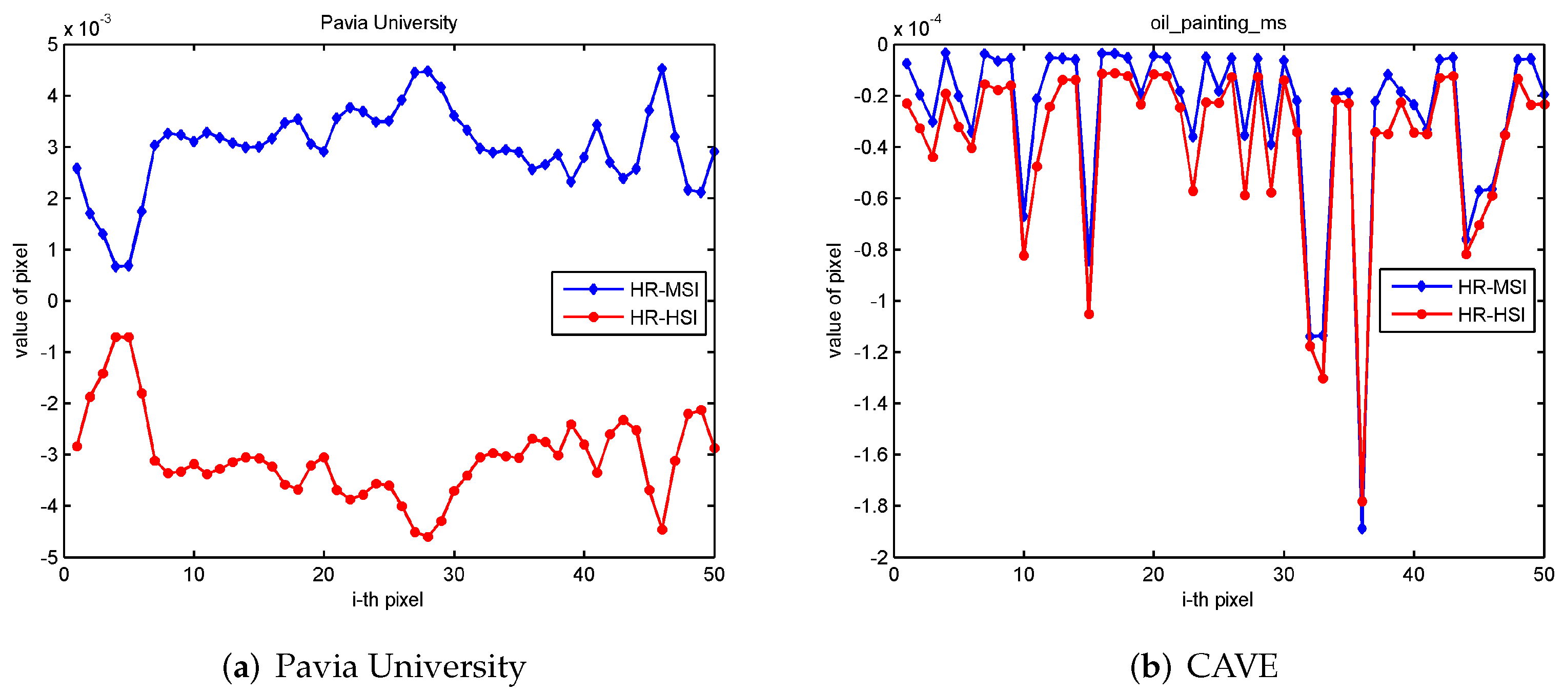
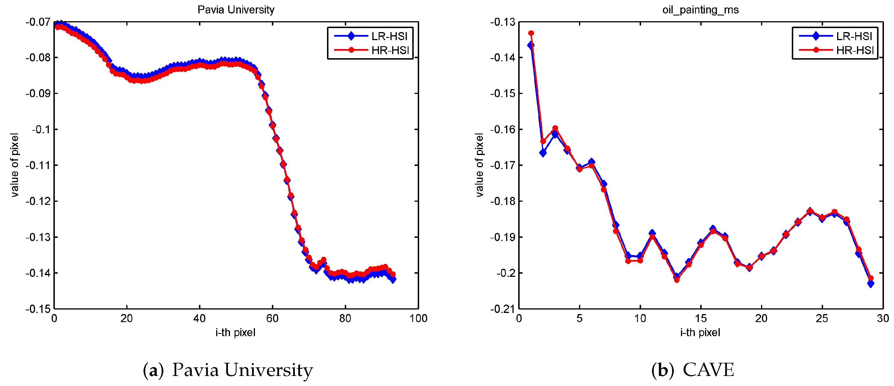
As shown in Figure 1, we found a strong correlation between HR-HSI and HR-MSI. The values of the third TMSVD factor matrix from the HR-MSI and HR-HSI are similar or opposite in the same position. As we can see from Figure 2, the first factor matrix value from HR-HSI and LR-HSI by TMSVD are also approximately the same at the same position, which can explain why the spectral basis comes from the LR-HSI based on matrix similarity, where there was previously no tangible evidence to explain this. We estimate the three SVD factor matrices of HR-HSI from LR-HSI and HR-MSI using TMSVD, and the three factor matrices are then used to construct the HR-HSI, which is different from estimating the spectral basis and the corresponding spectral coefficient matrix.

However, compared with SVD, TMSVD is limited by a truncated value. It only saves part of the original matrix information, which will cause the loss of some critical information. To further improve the fusion effect, we assume that the first TMSVD factor matrix of HR-MSI also contains some information about HR-HSI. Therefore, we introduce the first TMSVD factor matrix of HR-MSI into the fusion process.

We integrate the prior information of TMSVD on HR-MSI and LR-HSI to reconstruct HR-HSI, obtaining the factor matrices from LR-HSI and HR-MSI by TMSVD. We then recombine the obtained factor matrices to obtain a rough HR-HSI and, through a multiplicative iterative process, can finally solve the optimization question.

The main contributions of this paper are as follows:

• We explain that the reason for the spectral basis comes from LR-HSI from the perspective of the matrix similarity after truncated singular value decomposition. No such quantitative analysis has been conducted prior to our work.
• We found a strong correlation between HR-MSI and HR-HSI. All prior information about TMSVD was integrated into a new proposed fusion model without using the SRF and based only on the TMSVDfactor matrices from LR-HSI and HR-HSI.
• We propose a new idea for the hyperspectral fusion method. We reconstruct the HR-HSI by estimating the three SVD factor matrices of HR-HSI from LR-HSI and HR-MSI.
• We test our proposed method on two simulated data sets, Pavia University and CAVE, and a real data set in which the remote sensing images are generated by two different spectral cameras, Sentinel 2 and Hyperion. Compared with the non-blind methods, our proposed method achieves a more effective fusio result while reducing fusing time to less than 1% of such methods. Compared with the blind methods on the simulated data sets, our proposed method can improve the PSNR value by up to 16 dB. Moreover, our proposed method demonstrates a better performance on the real data set, which validates its practicality.

The rest of this paper is organized as follows. In Section 2, some background knowledge and the representative hyperspectral image super-resolution literature are presented. The FTMSVD method is presented in Section 3. The experimental details are outlined in Section 4. Presented in Section 5 are our experimental results and analysis, and the conclusion is found in Section 6.

2. Related Work

In recent years, the exploration of hyperspectral image (HSI) super-resolution methods has been gradually increasing. These methods can be broadly divided into three categories: matrix factorization-based methods, tensor factorization-based methods, and other methods.

In the matrix factorization-based methods, it is assumed that HR-HSI is a matrix formed by the multiplication of the spectral basis and the corresponding spectral coefficient matrix. The fusion problem is transformed into the problem of how to estimate the spectral basis and coefficient matrix. There are many ways to estimate the spectral basis and coefficient matrix, such as non-negative dictionary learning [13], K-SVD [14], and online dictionary learning [15]. Wycoff et al. [16] made full use of the prior information of non-negativity and sparsity of HR-HSI and conducted non-negative sparse matrix factorization for HR-MSI and LR-HSI to obtain the approximation of a non-negative spectral basis and sparse coefficient matrix, and the alternative direction multiplier method (ADMM) was then used in their optimization to obtain the HR-HSI. Akhtar et al. [17] estimated a non-negative dictionary based on the principle of local similarity of images. In [18], the spectral basis and coefficient matrix were learned from LR-HSI and MR-HSI under some prior information. Huang et al. [19] proposed obtaining the learning spectral basis by using K-SVD on LR-HSI. Han et al. [20] clustered image blocks and assumed that similar image blocks can linearly represent the given block, learning of the local similarity of HR-HSI was based on image segmentation. The method we propose in this paper is also a matrix factorization-based method. However, our FTMSVD method differs in two aspects. Firstly, in our FTMSVD method, information is directly obtained from LR-HSI and HR-MSI by TMSVD without the need for a complex operation such as dictionary learning. Secondly, in our proposed method, it is assumed that HR-HSI is composed of three SVD factor matrices, and we estimate the three SVD factor matrices of HR-HSI from LR-HSI and HR-MSI, but not the spectral basis and coefficient matrix.

Tensor factorization-based methods allow for preserving the 3D characteristics of hyperspectral images to a great extent. That is, tensors represent hyperspectral images, and the structure information of the image is better preserved. The question for fusion then concerns how to estimate the tensors. Dian et al. [21] used Tucker decomposition to decompose HR-HSI into three dictionaries of three dimensions and used a kernel tensor to describe the relationship between the dictionaries. Li et al. [22] proposed a method based on coupled sparse tensor representation (CSTF) in which HR-HSI is regarded as a three-dimensional tensor. The tensor could be approximated as a core tensor multiplied by three subtensors. In [11], subspace representation and low-rank tensor representation are combined. The spectral subspace is approximated by the singular value decomposition of LR-HSI, and the coefficients are estimated by the low-rank tensor. Prvost et al. [23] obtained the dictionary of the third modes by the operation of TMSVD, and they solved the generalized Sylvester equation to obtain the kernel tensor.

Other methods mainly include the Bayesian-based and deep convolutional neural network (CNN)-based methods. In the Bayesian-based methods, the prior distribution is used to solve the fusion problem. A representative example is the proposal in [24]. The method based on CNN also plays an important role in the realization of hyperspectral image fusion. Dong et al. [25,26] constructed a deep CNN for solving single image super-resolution and achieved excellent performance. Liu et al. [27] proposed a deep CNN named SSAU-Net, by introducing the spectral-spatial attention module to extract the shallow and deep features information from LR-HSI and HR-HSI. Work [28] cleverly combined subspace representation with CNN denoisier, which only need to train on the gray images. This method solves the difficult problem about the training for CNN model.

These methods are also roughly divided into two categories, depending on whether PSF and SRF are known during the fusion process, as blind fusion methods and non-blind fusion methods. Methods that are non-blind indicate that both PSF and SRF are known. On the contrary, PSF and SRF are unknown in blind methods. Hysure (blind version) [29] and CNMF [18] are blind methods in which the fusion process is achieved by estimating both SRF and PSF from HR-MSI and LR-HSI. The method in [30] is also a blind method because it only estimates the SRF and does not use the PSF during the fusion process. In either case, our proposed method demonstrates good performance without using SRF. When the PSF is known, we use it directly. If the PSF cannot be directly obtained, we can use the PSF that we set. Our experiments demonstrate that our method achieves good results in both cases.

3. Fusion Model

We denote the target HR-HSI as a three-dimensional tensor $\mathcal{Z}\in {\mathbb{R}}^{W\times H\times L}$, which has $W\times H$ pixels and L bands. The LR-HSI is regarded as $\mathcal{X}\in {\mathbb{R}}^{w\times h\times L}$, which has $w\times h$ pixels and L bands. $\mathcal{Y}\in {\mathbb{R}}^{W\times H\times l}$ represents the observed HR-MSI, with $W\times H$ pixels and l bands. It is observed that $w<W$, $h<H$, and $l<L$. $\mathcal{X}$ can be seen as a spatially downsampled version of $\mathcal{Z}$, i.e.,

$$\mathbf{X}=\mathbf{Z}\mathbf{BS}$$

(1)

where $\mathbf{X}\in {\mathbb{R}}^{L\times wh}$ and $\mathbf{Z}\in {\mathbb{R}}^{L\times WH}$ represent mode-n matricization matrix of $\mathcal{X}$ and $\mathcal{Z}$, respectively. The matrices $\mathbf{B}\in {\mathbb{R}}^{WH\times WH}$ and $\mathbf{S}\in {\mathbb{R}}^{WH\times wh}$ represent the convolutional blur and downsampling matrix, respectively. In a practical situation, the PSF represents $\mathbf{B}$, which is uncertain, and $\mathbf{S}$ can be obtained by the proportion of spatial dimensions of LR-HSI and HR-MSI.

The $\mathcal{Y}\in {\mathbb{R}}^{W\times H\times l}$ can also be seen as the spectral downsampling version of $\mathcal{Z}$, i.e.,

$$\mathbf{Y}=\mathbf{R}\mathbf{Z}$$

(2)

where $\mathbf{Y}\in {\mathbb{R}}^{l\times WH}$ and $\mathbf{R}\in {\mathbb{R}}^{l\times L}$ represent the mode-n matricization matrix of $\mathcal{Y}$ and the spectral response matrix, respectively. $\mathbf{R}$ represents the SRF, which is uncertain in most cases.

In [31], SVD was used for image compression, because it can denoise and represent most information of an image with a few elements. Therefore, if we can obtain the three SVD factor matrices of $\mathbf{Z}$, we can recover the original HR-HSI, i.e.,

$$\mathbf{Z}=\mathbf{U}\mathbf{\Sigma }{\mathbf{V}}^T$$

(3)

where ${\mathbf{U}}_z\in {\mathbb{R}}^{L\times d}$, ${\mathbf{\Sigma }}_z\in {\mathbb{R}}^{d\times d}$ and ${\mathbf{V}}_z^T\in {\mathbb{R}}^{d\times WH}$ are the corresponding factor matrices of Z by SVD. However, it is difficult to directly obtain the SVD factor matrices of $\mathbf{Z}$. To approximate the SVD factor matrices of $\mathbf{Z}$, we estimate the SVD factor matrices of $\mathbf{Z}$ from $\mathbf{X}$ and $\mathbf{Y}$ by using TMSVD, i.e.,

$$\mathbf{Z}={\mathbf{U}}_z{\mathbf{\Sigma }}_z{\mathbf{V}}_z^T$$

(4)

where ${\mathbf{U}}_z\in {\mathbb{R}}^{L\times q}$, ${\mathbf{\Sigma }}_z\in {\mathbb{R}}^{q\times q}$, and ${\mathbf{V}}_z^T\in {\mathbb{R}}^{q\times WH}$ are the corresponding estimation factor matrices obtained by TMSVD, and $\mathbf{q}$ is the truncated value. Therefore, Equations (1) and (2) can be converted to the following equation.

$$\mathbf{X}={\mathbf{U}}_z{\mathbf{\Sigma }}_z{\mathbf{V}}_z^T\mathbf{B}\mathbf{S}$$

(5)

$$\mathbf{Y}=\mathbf{R}{\mathbf{U}}_z{\mathbf{\Sigma }}_z{\mathbf{V}}_z^T$$

(6)

The fusion problem turns into the problem of estimating three factor matrices ${\mathbf{U}}_z$, ${\mathbf{\Sigma }}_z$, and ${\mathbf{V}}_z^T$ from HR-MSI and LR-HSI. To distinguish it from the target matrix $\mathbf{Z}$, we denote ${\mathbf{Z}}_s$ as the fusion matrix, i.e.,

$${\mathbf{Z}}_s={\mathbf{U}}_s{\mathbf{\Sigma }}_s{\mathbf{V}}_s^T$$

(7)

where ${\mathbf{U}}_s\in {\mathbb{R}}^{L\times q}$, ${\mathbf{\Sigma }}_s\in {\mathbb{R}}^{q\times q}$ and ${\mathbf{V}}_s^T\in {\mathbb{R}}^{q\times WH}$ are the corresponding factor matrices of fusion result ${\mathbf{Z}}_s$ by TMSVD. Since $l<L$, the truncated singular value $\mathbf{q}$ is constrained below l, and we set l as the truncated singular value for the consistency of TMSVD factor matrix dimensions. Through performing the TMSVD operation on $\mathbf{Y}$ and $\mathbf{X}$ with truncated value $\mathbf{q}$, we can obtain the TMSVD factor matrices of $\mathbf{Y}$ and $\mathbf{X}$, respectively, i.e.,

$$\mathbf{Y}={\mathbf{U}}_y{\mathbf{\Sigma }}_y{\mathbf{V}}_y^T$$

(8)

$$\mathbf{X}={\mathbf{U}}_x{\mathbf{\Sigma }}_x{\mathbf{V}}_x^T$$

(9)

where ${\mathbf{U}}_y\in {\mathbb{R}}^{l\times q}$, ${\mathbf{\Sigma }}_y\in {\mathbb{R}}^{q\times q}$ and ${\mathbf{V}}_y^T\in {\mathbb{R}}^{q\times WH}$, and ${\mathbf{U}}_x\in {\mathbb{R}}^{L\times q}$, ${\mathbf{\Sigma }}_x\in {\mathbb{R}}^{q\times q}$ and ${\mathbf{V}}_x^T\in {\mathbb{R}}^{q\times wh}$. They are the corresponding TMSVD factor matrices of X and Y.

As shown in Figure 1 and Figure 2, $|{\mathbf{V}}_y^T|\approx |{\mathbf{V}}_z^T|$ and ${\mathbf{U}}_x\approx {\mathbf{U}}_z$, and it was found in [12] that ${\mathbf{\Sigma }}_z\approx sf\times {\mathbf{\Sigma }}_x$, where $sf$ is the downsampling factor. Hence, we can obtain the following equations.

$${\mathbf{U}}_s={\mathbf{U}}_y$$

(10)

$${\mathbf{\Sigma }}_s=sf\times {\mathbf{\Sigma }}_x$$

(11)

$${\mathbf{V}}_s^T={\mathbf{V}}_y^T$$

(12)

However, constrained by the spectral dimension of HR-MSI, the $\mathbf{q}$ value is limited in l. Therefore, if we use ${\mathbf{U}}_s$, ${\mathbf{\Sigma }}_s$ and ${\mathbf{V}}_s^T$ to reconstruct HR-HSI, much important information about HR-HSI will be lost, and the fusion effect is unsatisfactory. Due to the features of SVD, ${\mathbf{U}}_y$ also obtains information of $\mathbf{Y}$, and $\mathbf{Y}$ contains most of the spatial information of $\mathbf{Z}$, so we introduce it in the reconstruction of ${\mathbf{V}}_s^T$ to improve the fusion performance, i.e.,

$${\mathbf{V}}_s^T={\mathbf{U}}_y\times {\mathbf{V}}_y^T$$

(13)

The detailed process for estimating the SVD factor matrices of HR-HSI is presented in Algorithm 1.

Based on Equations (1) and (9), we can further optimize the quality of ${\mathbf{Z}}_s$ as the following equation, i.e.,

$$\underset{{\mathbf{U}}_s{\mathbf{\Sigma }}_s{\mathbf{V}}_s^T}{min}{∥\mathbf{X}-{\mathbf{U}}_s{\mathbf{\Sigma }}_s{\mathbf{V}}_s^T\mathbf{B}\mathbf{S}∥}_F^2$$

(14)

where ${\parallel \mathbf{A}\parallel }_F^2$ means the Frobenius norm of $\mathbf{A}$ in this paper.

Algorithm 1 Estimate three rough SVD factor matrices of HR-HSI

Require:$\mathcal{X}$$\mathcal{Y}$ obtain the downsampling factor $sf$ and the truncated value q from $\mathcal{X}$ and $\mathcal{Y}$ $[nr,\sim ,q]=size(\mathcal{Y})$ $[n{r}_1,\sim ,\sim ]=size(\mathcal{X})$ $sf=nr/n{r}_1$ Matrix $\mathcal{X}$ and $\mathcal{Y}$ to $\mathbf{X}$ and $\mathbf{Y}$ The truncated singular value decomposition on $\mathbf{X}$ and $\mathbf{Y}$ with truncated value q $\left[{\mathbf{U}}_x,{\mathbf{\Sigma }}_x,\sim \right]=SVD(\mathbf{X},q)$ $\left[{\mathbf{U}}_y,\sim ,{\mathbf{V}}_y^T\right]=SVD(\mathbf{Y},q)$ ${\mathbf{U}}_s={\mathbf{U}}_x$ ${\mathbf{\Sigma }}_s=sf\times {\mathbf{\Sigma }}_x$ ${\mathbf{V}}_s^T={\mathbf{U}}_y{\mathbf{V}}_y^T$ return${\mathbf{U}}_s,{\mathbf{\Sigma }}_s,{\mathbf{V}}_s^T$

Because of the correlation in Figure 1 and [12], we assume that ${\mathbf{\Sigma }}_s$ and ${\mathbf{V}}_s^T$ are approximately equal to ${\mathbf{\Sigma }}_z$ and ${\mathbf{V}}_z^T$, which means ${\mathbf{\Sigma }}_s$ and ${\mathbf{V}}_s^T$ are fixed during the fusion process. We therefore simplify Equation (14), i.e.,

$$\underset{{\mathbf{U}}_s}{min}{∥\mathbf{X}-{\mathbf{U}}_s\mathbf{C}∥}_F^2$$

(15)

We set $\mathbf{C}={\mathbf{\Sigma }}_s{\mathbf{V}}_s^T\mathbf{B}\mathbf{S}$ as constant throughout the fusion process. The meaning of $\mathbf{C}$ here is similar to the coefficient matrix in the work [11], except that we get it directly by the connection between HSI and MSI, without any additional operations. Note that there are two cases of $\mathbf{B}$. If PSF is known in practice, we use it directly. If PSF is unknown, we use the one we set, which is a $5\times 5$ Gaussian blur (standard deviation 1) in this paper, and solve the uncertainty of $\mathbf{B}$ in this way. Finally, a multiplicative iterative process as in [18] is introduced to optimize ${\mathbf{U}}_s$ in Equation (15), i.e.,

$${\mathbf{U}}_s={\mathbf{U}}_s.\times (\mathbf{X}{\mathbf{C}}^T)./({\mathbf{U}}_s\mathbf{C}{\mathbf{C}}^T)$$

(16)

After several iterative rounds of optimization, we obtain a more accurate ${\mathbf{U}}_s$. We reconstruct it using ${\mathbf{\Sigma }}_s$ and ${\mathbf{V}}_s^T$ to obtain a satisfactory $\mathbf{Z}$. The whole process of our method is shown in Algorithm 2.

Algorithm 2 FTMSVD Algorithm

Require:$\mathcal{X}$$\mathcal{Y}$ Obtain the ${\mathbf{U}}_s$${\mathbf{\Sigma }}_s$${\mathbf{V}}_s^T$ via TMSVD with a truncated singular value q in Algorithm 1 if PSF is known then    Use it directly else [PSF is unknown]    Set PSF as a $5\times 5$ Gaussian blur (standard deviation 1) end if Set $\mathbf{C}={\mathbf{\Sigma }}_s{\mathbf{V}}_s^T\mathbf{B}\mathbf{S}$ ${\mathbf{Z}}_f={\mathbf{U}}_s\mathbf{C}$ Use a multiplicative iterative processe to optimize the ${\mathbf{U}}_s$ for k = 1:K do    Update ${\mathbf{U}}_s$ by Equation (16) end for ${\mathbf{Z}}_f={\mathbf{U}}_s{\mathbf{\Sigma }}_s{\mathbf{V}}_s^T$ $\mathbf{Z}={\mathbf{Z}}_f$ return$\mathbf{Z}$

4. Experiments

4.1. Data Set

To demonstrate the universality and effectiveness of our proposed FTMSVD method, we conduct experiments on two simulated data sets, the CAVE [32] and Pavia University [33] data sets. In addition, we test our proposed method on a real data set of remote sensing images generated by Sentinel 2 and Hyperion spectral cameras.

In the CAVE data set, each HSI has $512\times 512$ pixels and 31 spectral bands and consists of 32 indoor scenes with high quality and a spectral range from 400 to 700 nm. We removed the final two fuzzy bands and kept the remaining 29 bands. The Pavia University data set was acquired by the ROSIS sensor, which has $610\times 340$ space pixels with 115 spectral bands (0.43–0.86 $\mathsf{\mu }$m) from around Pavia University, northern Italy. We removed the final fuzzy bands and kept the remaining 93 bands to use the upper left corner ($256\times 256\times 93$). Compared with non-blind methods, we filter each HR-HSI band with the $7\times 7$ Gaussian blur (standard deviation 2) and conduct downsampling every 32 pixels in two spatial modes to simulate the LR-HSI in the simulated data sets. The HR-MSIs of the Pavia University data set are obtained using the IKONOS class reflection spectral response filter [34]. The HR-MSIs (RGB image) from the CAVE data set are generated by a Gf-1-16m multispectral camera response function. Specifically, for the Pavia University data set, each LR-HSI is $8\times 8\times 93$ and HR-MSI is $256\times 256\times 4$. For the CAVE data set, the LR-HSI is $16\times 16\times 29$ and the HR-MSI is $512\times 512\times 3$. For comparison, we set the downsampling as 8 for blind methods and kept other settings the same as for non-blind in generating the LR-HSI ($32\times 32\times 93$) and the LR-HSI ($64\times 64\times 29$) from the Pavia University and CAVE data sets, respectively. The HR-MSIs are the same as in non-blind fusion processes.

For the real remote sensing data set, the LR-HSI was obtained by the Hyperion sensor on the Earth Observation 1 satellite, which has 220 spectral bands. Our experiments use one part of it as the LR-HSI ($100\times 100\times 89$). The corresponding HR-MSI is $300\times 300\times 4$, generated by the Sentinel-2A satellite.

All experiments were implemented in MATLAB R2014a on localhost with 2.90 GHz Intel i5-9400F CPU and 8.0 GB DDR3.

4.2. Experimental Settings

To demonstrate the superiority of our proposed method in different situations (non-blind and blind), we organize the experiments in the following order.

First of all, through two simulated data sets, we compare our proposed method with five state-of-the-art non-blind fusion methods, including Hysure(NB) (non-blind version) [29], CSTF [22], STEREO(NB) (non-blind version) [35], NLSTF [21], and LTTR [36]. We chose the parameters to obtain the best performance for each method in different data sets when the downsampling factor is 32. The experiment results demonstrate that our method results in a better performance in less execution time. The specific parameters of the five state-of-the-art methods are given below in

Table 1. Parameters of non-blind methods on the Pavia University data set.

Method	Parameters
Hysure(NB)	basis = ’VCA’, ${\lambda }_{\phi }=1\times {10}^{-7}$, ${\lambda }_m=1\times {10}^3$, ${\lambda }_B={\lambda }_R=10$, mu = 0.05, iters = 200
CSTF	$n_w=400$, $n_h=400$, $n_s=8$, and $\lambda =1\times {10}^{-6},$$\beta =0.001$, K = 20
STEREO(NB)	$\lambda =1\times {10}^{-3}$, $s\_iter=2$, $t\_rank=40$, $maxit=5$, $kernel\_length=21$
NLSTF	$W=H=10$, $S=14$, $K=151$, $\lambda =1\times {10}^{-6}$, ${\lambda }_1={\lambda }_2={\lambda }_3=1\times {10}^{-5}$
LTTR	$K=3900$, $eta=0.002$

and

Table 2. Parameters of non-blind methods on the CAVE data set.

Method	Parameters
Hysure(NB)	basis = ’VCA’, ${\lambda }_{\phi }=1\times {10}^{-1}$, ${\lambda }_m=1\times {10}^5$, ${\lambda }_B={\lambda }_R=10$, mu = 0.05, iters = 200
CSTF	$n_w=400$, $n_h=400$, $n_s=10$, and $\lambda =1\times {10}^{-5}$, $\beta =0.001$, K = 20
STEREO(NB)	$\lambda =1\times {10}^{-4}$, $s\_iter=1$, $t\_rank=40$, $maxit=100$, $kernel\_length=31$
NLSTF	$W=H=10$, $S=14$, $K=151$, $\lambda =1\times {10}^{-6}$, ${\lambda }_1={\lambda }_2={\lambda }_3=1\times {10}^{-5}$
LTTR	$K=760$, $eta=0.0009$

.

Secondly, we verify the validity of ${\mathbf{V}}_s^T$ extracted from our finding in Figure 1 by using a randomly selected factor matrix to replace ${\mathbf{V}}_s^T$ and intuitively display the influence of ${\mathbf{V}}_s^T$.

We then compare our proposed method with five state-of-the-art blind methods on two simulated data sets, in which the LR-HSI and HR-MSI are simulated based on different SRF and PSF values. The compared blind methods we used include the Hysure (https://github.com/alfaiate/HySure/ (blind version) accessed on 1 October 2022) [29], CNMF [18], GSA [37], SFIMHS [38], and MAPSMM [39]. Our proposed FTMSVD method, GSA, and SFIMHS do not require additional setting parameters. In fact, it is very difficult to debug the optimal parameters in the real blind fusion scenario, so we keep the parameter settings of Hysure, CNMF, and MAPSMM in the original literature for a realistic and reliable comparison in blind fusion experiments.

After that, we will use the different PSF to replace the one we set in our proposed method to show the impact of the fixed PSF and to further illustrate the generalization of our proposed method.

Finally, we take the experiment on the real data set and show the fusion visual fidelity.

4.3. Quantitative Metrics

To evaluate the effectiveness of our proposed method in all aspects, we use subjective and objective evaluation metrics. For the subjective metrics, we show the effectiveness of our proposed method through the visual presentation of the fused images. We used six objective indexes to simultaneously reflect the fusion results. Regarding the peak signal-to-noise ratio (PSNR) [11], the larger the value of PSNR, the better the spatial reconstruction quality of each band; regarding the Erreur Relative Globale Adimensionnelle de Synthese (ERGAS) [40], the smaller the ERGAS, the better the overall quality of the fused image; regarding spectral angle mapper (SAM) [34], the smaller the SAM, the better the quality of fusion; regarding the structural similarity (SSIM) [41], which is used to evaluate the similarity of two images by brightness, contrast, and structure, the closer the metric is to 1, the better the effect; regarding the universal Image Quality Index (UIQI) [42], which is used to address simultaneously spectral and radiometric quality, the closer the UIQI is to 1 the better result and regarding fusion time, which is used to evaluate the speed of the fusion method, the smaller the value, the faster the fusion.

5. Results and Analysis

5.1. Compared with Non-Blind Methods

The results of the non-blind situation are shown in

Table 3. Average quantitative results of the non−blind methods on the Pavia University data set.

Method	PSNR	ERGAS	SAM	UIQI	SSIM	TIME
Hysure(NB)	42.494	0.154	2.205	0.992	0.988	54.925
CSTF	43.077	0.144	2.140	0.993	0.989	258.772
STEREO(NB)	27.263	0.792	8.732	0.772	0.696	1.370
NLSTF	29.556	0.672	7.382	0.924	0.936	60.850
LTTR	32.438	0.676	7.675	0.908	0.932	236.399
FTMSVD	43.168	0.140	2.049	0.993	0.989	0.287

and

Table 4. Average quantitative results of the non−blind methods on the CAVE data set.

Method	PSNR	ERGAS	SAM	UIQI	SSIM	TIME
Hysure(NB)	40.138	0.423	15.350	0.934	0.956	220.819
CSTF	40.674	0.463	8.032	0.914	0.957	335.912
STEREO(NB)	31.348	0.690	16.927	0.739	0.837	16.549
NLSTF	24.648	1.518	14.377	0.717	0.814	185.460
LTTR	33.947	1.219	13.132	0.790	0.906	319.596
FTMSVD	41.115	0.387	13.916	0.937	0.959	0.835

, and the values in bold are the best results in the metric. All the data values in the table are the average of the five experiments. For visual comparison, we introduce the image of the experimental results for comparison. Figure 3 and Figure 4 are the corresponding images. Table 3 shows the average objective metrics on the Pavia University data set. Our FTMSVD method has the best performance compared with other non-blind methods on all objective metrics, which means that HR-HSI reconstructed by our FTMSVD method has the best spatial and spectral qualities. More specifically, the PSNR of our FTMSVD method is higher than that of CSTF method by 0.091 dB, but we reduce the execution time by about 258.485 s. From Table 4, it can be seen that our proposed method achieves the best result on the CAVE data set. The main improvement reason is that our method extracts the reconstruction information from $\mathbf{X}$ and $\mathbf{Y}$ based directly on TMSVD and without complex operations. The optimization we used is multiplicative iterative processes, which only optimize the ${\mathbf{U}}_s$ in a short time. The reason why the optimization is so fast is because the optimize process only works on smaller matrices ${\mathbf{U}}_s$. Most matrix-based fusion methods take a large amount of time because they need to optimize both the spectral subspace and the corresponding coefficient matrix. In [11], the approximate estimation of subspace through LR-HSI can reduce the operation, but the coefficient matrix is still very large, and the fusion time is long. The data volume of the coefficient matrix is much larger than the spectral base. Due to the discovery of Figure 1, we can make an approximate substitution of the last two SVD factor matrices of HR-HSI by combining the work [12] with our findings. Therefore, we propose the optimization method in Equation (15) only need to optimize a smaller matrix.

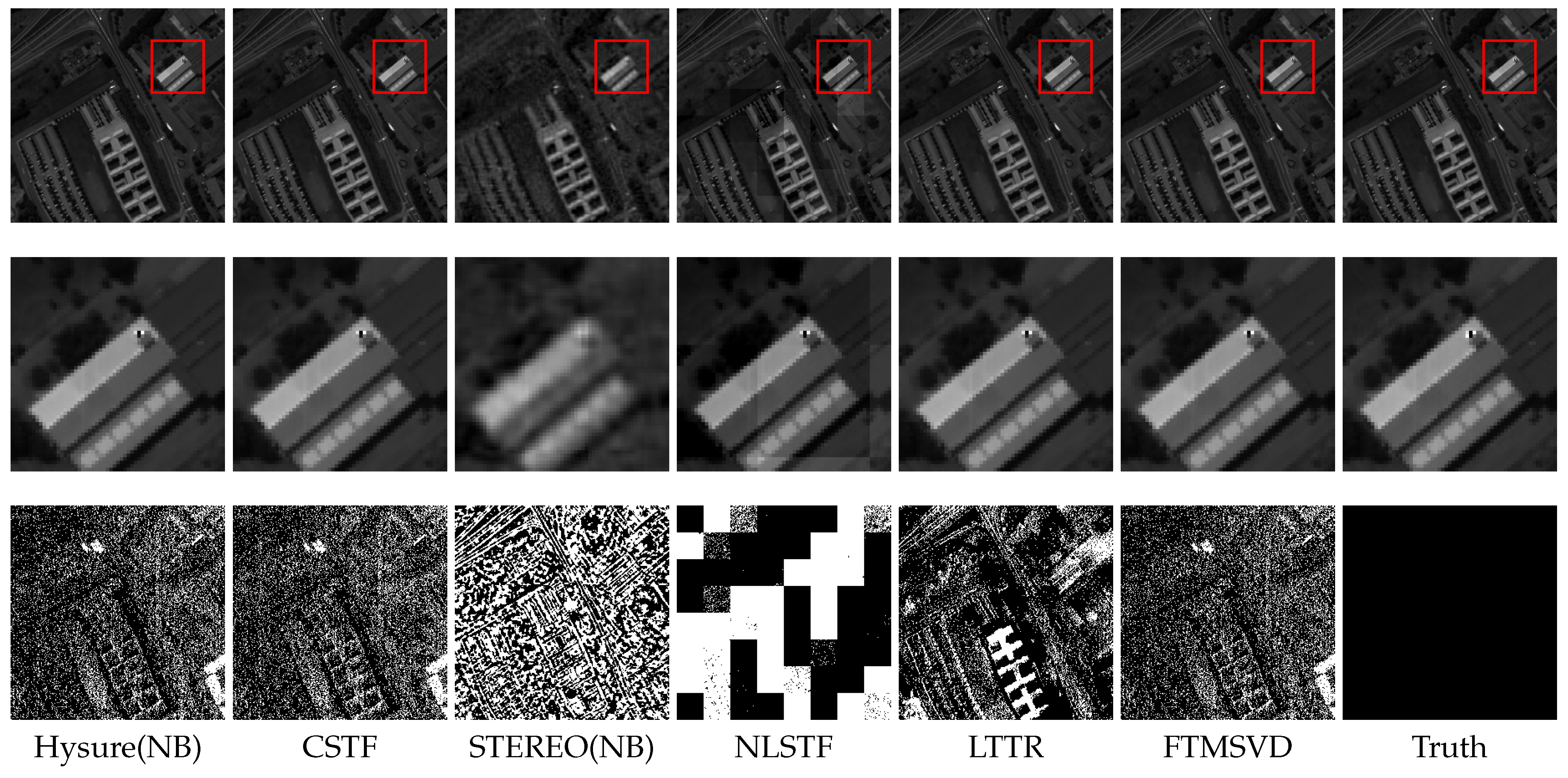
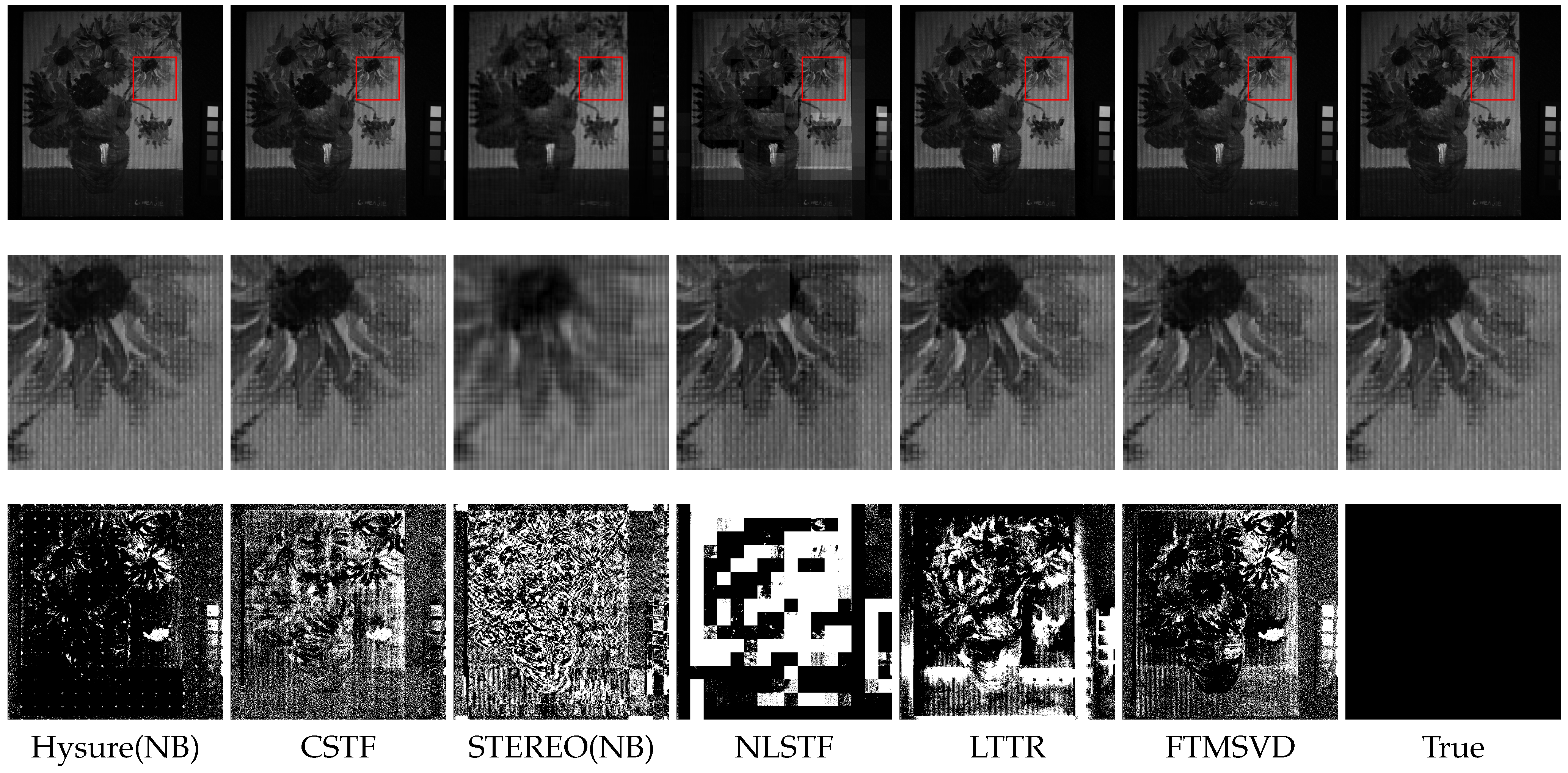
As we can see from Figure 3 and Figure 4, the first row shows the fused images of each method at band 30, and the second row is the enlarged one of the marked area in the first row. The third row shows the error images at band 30, and the more black pixels there are, the closer the fused image is to the ground true image. Take a comprehensive view from Figure 3, when the downsampling factor is 32, the Hysure(NB), CSTF and our proposed method FTMSVD have the better visual effect than STEREO(NB), NLSTF and LTTR. Although the error images of the Hysure(NB) appears to perform better than FTMSVD on the CAVE data set, the FTMSVD still has a better performance than others. In combination with Table 3 and Table 4, FTMSVD method has better performance on both data sets.

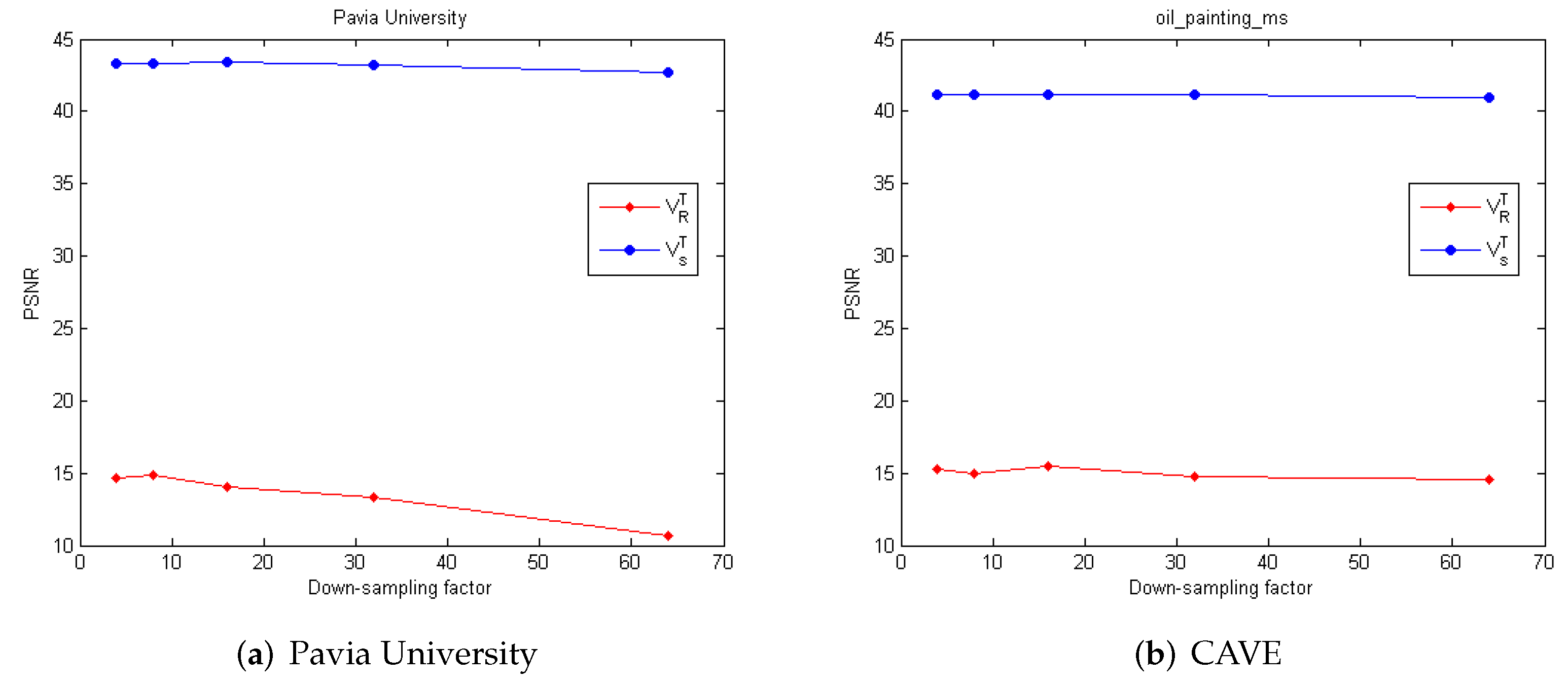
5.2. Impact of the ${\mathbf{V}}_s^T$ to Fusion Effect

Here, we use a randomly selected factor matrix ${\mathbf{V}}_R^T$ to replace ${\mathbf{V}}_s^T$ in Algorithm 1 to verify the impact of our finding in Figure 1 on the fusion result. Figure 5 shows the PSNR values in two simulated data sets. One uses ${\mathbf{V}}_s^T$ and the other uses ${\mathbf{V}}_R^T$. We can see that in using ${\mathbf{V}}_R^T$, the value of PSNR is very low in the two data sets, which indicates poor fusion effect. The PSNR is much higher when using ${\mathbf{V}}_s^T$ in all data sets, which verifies that ${\mathbf{V}}_s^T$ can be effectively used to improve the fusion performance, and the improvement effect is pronounced. The main reason for this result is that ${\mathbf{V}}_s^T$ is directly obtained from the truncated singular value decomposition on HR-MSI, which contains large spatial information of HR-MSI. Due to the HR-MSI being a spectral downsampling of HR-HSI, ${\mathbf{V}}_s^T$ is a better approximation of ${\mathbf{V}}_z^T$. Therefore, we can obtain a better fusion result by using ${\mathbf{V}}_s^T$ to reconstruct HR-HSI.

5.3. Comparison with Blind Methods

To comprehensively evaluate the superiority of our proposed method in blind fusion cases, we compare it with five state-of-the-art blind methods in this section. To make a more direct comparison, we will compare the two simulated data sets, in which the HR-HSI (which we obtain) can be compared with the fusion results of blind methods in terms of objective metrics. We exchange the PSF of CAVE and Pavia University to generate six LR-HSI and HR-MSI pairs. Here, we refer to the IKONOS class reflection spectral response filter as SRF1 and the Gf-1-16m multispectral camera response as SRF2. The $7\times 7$ Gaussian blur (standard deviation 2) is defined as PSF1, and the $3\times 3$ average blur is PSF2. Different combinations of these are used to generate the LR-HSI and the HR-MSI. We keep the PSF1 for the Pavia University data set and only use different SRFs. We change both the SRF and the PSF for the CAVE data set. The downsampling factor is 8. We compared the blind methods on the simulated data sets according to the objective fusion metrics, and the image of the fusion result of some data sets is visually displayed.

Table 5. Average quantitative results of the blind methods on the Pavia University data set.

SRF & PSF	Method	PSNR	ERGAS	SAM	UIQI	SSIM	TIME
SRF1 PSF1	Hysure	38.180	0.958	3.007	0.986	0.981	52.678
	CNMF	26.323	3.527	6.099	0.824	0.805	14.823
	GSA	27.599	3.152	8.029	0.919	0.910	0.882
	MAPSMM	23.144	5.412	8.061	0.701	0.715	40.453
	SFIMHS	23.974	4.959	6.831	0.766	0.778	0.301
	FTMSVD	40.122	0.740	2.357	0.990	0.987	0.356
SRF1 PSF2	Hysure	36.445	1.148	3.264	0.980	0.974	53.378
	CNMF	24.638	4.201	7.842	0.781	0.741	15.305
	GSA	24.262	4.593	11.461	0.864	0.836	0.790
	MAPSMM	21.634	6.349	9.348	0.586	0.617	41.387
	SFIMHS	22.503	5.822	8.038	0.699	0.727	0.197
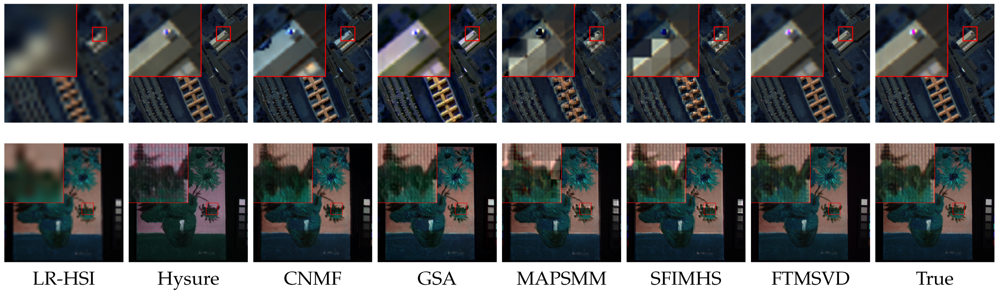
	FTMSVD	43.274	0.548	2.014	0.994	0.989	0.380

shows the fusion result on the Pavia University data set. As we can see, our proposed method achieved the best performance on most metrics in either case. The PSNR value of our proposed method is much better than other blind methods, where the maximum PSNR reached is almost 16 dB, and the minimum is almost 5 dB. The improvement in PSNR demonstrates the superiority of our proposed method in the blind fusion effect. Although the fusion time of our proposed method is not the best, it can still achieve the second best fusion time, which is only slightly longer than the time for the best performance.

Table 6. Average quantitative results of the blind methods on the CAVE data set.

SRF & PSF	Method	PSNR	ERGAS	SAM	UIQI	SSIM	TIME
SRF1 PSF1	Hysure	28.801	3.619	19.493	0.799	0.851	230.795
	CNMF	30.735	3.251	7.411	0.792	0.874	54.099
	GSA	33.646	2.262	10.210	0.875	0.910	1.061
	MAPSMM	27.069	4.563	7.949	0.738	0.849	173.955
	SFIMHS	26.309	5.136	6.834	0.797	0.880	0.276
	FTMSVD	40.438	1.044	6.270	0.950	0.972	0.840
SRF1 PSF2	Hysure	26.977	4.463	22.177	0.740	0.805	243.398
	CNMF	27.908	4.422	8.220	0.730	0.825	59.904
	GSA	32.708	2.482	11.918	0.850	0.878	1.111
	MAPSMM	26.093	5.095	8.784	0.662	0.813	166.409
	SFIMHS	25.580	5.484	7.408	0.766	0.864	0.257
	FTMSVD	41.614	0.964	5.147	0.954	0.979	0.961
SRF2 PSF1	Hysure	35.563	1.740	8.274	0.922	0.955	256.527
	CNMF	31.860	2.630	7.276	0.817	0.896	51.648
	GSA	34.974	1.967	9.306	0.898	0.926	1.066
	MAPSMM	27.186	4.450	7.875	0.786	0.870	140.832
	SFIMHS	26.792	4.664	6.533	0.813	0.885	0.250
	FTMSVD	40.806	1.542	13.995	0.938	0.959	0.852
SRF2 PSF2	Hysure	35.344	1.795	8.126	0.919	0.953	249.050
	CNMF	29.929	3.395	8.131	0.772	0.867	45.055
	GSA	33.665	2.221	10.838	0.876	0.899	1.017
	MAPSMM	26.235	4.962	8.388	0.741	0.849	138.072
	SFIMHS	25.778	5.240	7.168	0.773	0.865	0.213
	FTMSVD	41.123	1.535	13.977	0.938	0.959	0.733

shows the experimental results on the CAVE data set. Our proposed method achieves the best result on all metrics except fusion time. In the case of SRF1 and PSF2, our proposed method can achieve 43.274 dB for PSNR, while the second best is only 36.445 dB. The fusion time of our proposed method is still a little longer than that of SFIMHS, but the PSNR value of SFIMHS is only 22.503 dB. From Table 5 and Table 6, our proposed method is seen to be significantly better than other methods in terms of fusion quality. Due to page limitations, we only show the fusion images using the SRF1 and PSF1 on both data sets. Figure 6 are the fusion images of six blind methods on two data sets. In the upper left corner of each image is an enlargement of the portion marked in that image. From the performance on the two data sets in Figure 6, we can intuitively see from the visual fidelity that the image produced from our method is closer to the original image than those of other compared blind methods. From Figure 6, we can intuitively see that our fusion effect is closer to the original image than other compared blind methods. The main reason is that the information we extract from LR-HSI and HR-MSI can effectively simulate the corresponding three SVD factor matrices of HR-HSI, which saves the primary spectral information of LR-HSI and the main spatial information of HR-MSI. In addition, the method is independent of SRF, which allows avoiding the error and the time cost associated with SRF estimation. In addition, our proposed method does not depend on SRF, which can avoid the error of estimating the SRF and save a lot of fusion time.

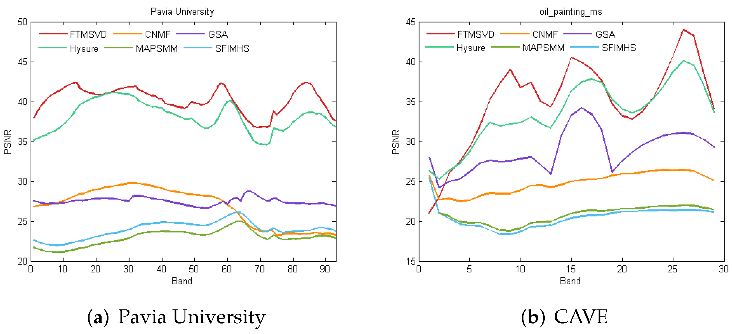
To further contrast the superiority of our method, we compare the performance of the compared methods in each spectral band. Figure 7 shows the change of PSNR for each spectral band over two data sets. As we can see from Figure 7a, the FTMSVD has the best performance than the other methods in each band. Figure 7b shows that the FTMSVD performs better than the compared methods at the most of the spectral bands. A higher PSNR value means that the spectral reflectance of the fusion result is more similar to the ground truth, which further demonstrates the advantages of our method.

5.4. The Impact of the PSF Set in the FTMSVD Method

Table 7. The results of the different PSF set in FTMSVD on the Pavia University data set.

Method	PSNR	ERGAS	SAM	UIQI	SSIM	TIME
PSFS1	40.122	0.740	2.357	0.990	0.987	0.453
PSFS2	42.976	0.559	2.044	0.993	0.990	0.228
PSFS3	42.473	0.591	2.090	0.993	0.988	0.255
PSFS4	43.000	0.564	2.040	0.993	0.989	0.211
PSFS5	42.529	0.591	2.043	0.993	0.989	0.203

and

Table 8. The results of the different PSF set in FTMSVD on the CAVE data set.

Method	PSNR	ERGAS	SAM	UIQI	SSIM	TIME
PSFS1	40.438	1.044	6.270	0.950	0.972	0.994
PSFS2	41.431	0.977	5.478	0.955	0.978	0.737
PSFS3	41.448	0.987	5.089	0.953	0.977	0.818
PSFS4	41.544	0.976	5.084	0.954	0.978	0.792
PSFS5	41.171	0.994	5.507	0.955	0.978	0.804

show the impact of different typical blur types as PSF set in our method. The data sets we used are the same as in Table 5 and Table 6 with SRF1 and PSF1. PSFS1 is the $5\times 5$ Gaussian blur (standard deviation 1) (which we used in this paper), PSFS2 is the $5\times 5$ average blur, PSFS3 is the $7\times 7$ average blur, PSFS4 is the $9\times 9$ Gaussian blur (standard deviation 2), and PSFS5 is the motion blur (len is 9 and theta is 0).

As we can see from Table 7 and Table 8, the PSF set in our proposed method can influence the fusion effect, but no matter which PSF we used, the fusion result is better than for the five compared blind methods in Table 5 and Table 6. The main reason is that the PSF is only used to optimize the first SVD factor matrix ${\mathbf{U}}_s$, and ${\mathbf{U}}_s$ mainly contains the spectral information of HR-HSI, and its size of is smaller than ${\mathbf{V}}_s^T$. For different PSF, the optimization effect of ${\mathbf{U}}_s$ is not significantly different. Moreover, most spatial information of HR-HSI is in ${\mathbf{\Sigma }}_s$ and ${\mathbf{V}}_s^T$ and unaffected by PSF. In this way, our proposed method only needs to assume a fixed PSF to replace its estimation. A multiplicative iterative process is then used to optimize ${\mathbf{U}}_s$, which can take a concise time to converge, so our proposed method can achieve a good fusion result within a short time.

5.5. Practicality of the Proposed Method

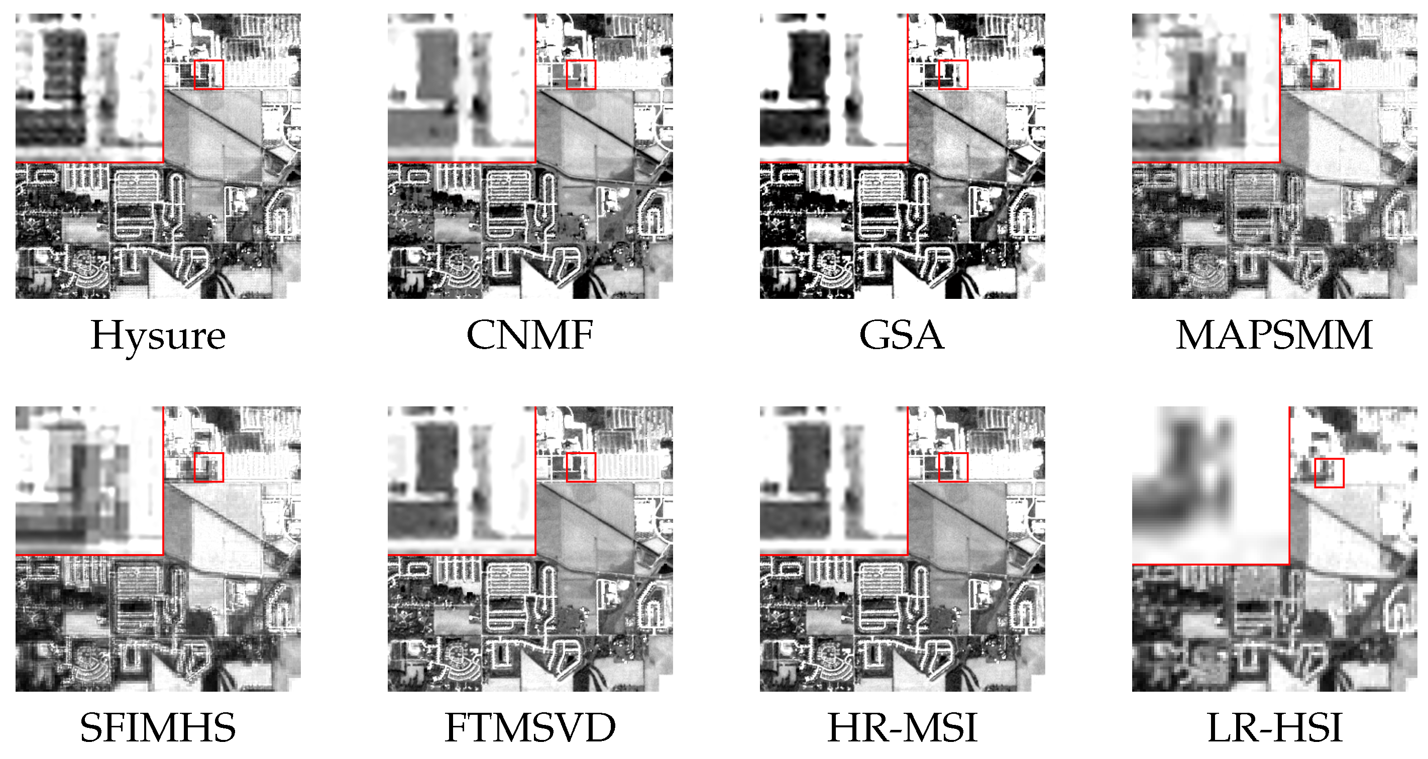
To demonstrate the practicality of our proposed method, we test our method with the five blind methods on the real remote sensing data set. The LR-HSI ($100\times 100\times 89$) and HR-MSI ($300\times 300\times 4$) are extracted from the real remote sensing data set. Figure 8 shows the LR-HSI, HR-MSI, and the corresponding fusion images of the different blind methods with enlargement of the marked position. Since the HR-HSI of the real data set is unknown, we directly compared the fusion effect from the fusion images. As Figure 8 shows, our proposed method has a better visual fidelity than others, and it is closer to the HR-MSI, which demonstrates its practicality.

6. Conclusions

In this paper, we find a strong correlation between the HR-MSI and HR-HSI. We experimentally verified the reason why the basic spectral values can be estimated from LR-HSI. We propose a fast fusion method based on TMSVD without SRF to implement the process of HR-MSI and LR-HSI fusion, which is suitable for both non-blind and blind fusion situations. Since LR-HSI contains the most spectral information of HR-HSI, the spatial information is mainly in HR-MSI. We estimated the SVD factor matrices of HR-HSI from HR-MSI and LR-HSI by TMSVD. Our proposed method solves the problems associated with the uncertainty of PSF and SRF, and a satisfactory fusion result can be rapidly produced. Our experimental results on the simulated hyperspectral data sets and real remote sensing data set all indicate the superiority of our proposed method. However, our pre-set PSF still has a slight impact on the fusion results of our proposed methods. Therefore, it is necessary for us to estimate a more suitable PSF based on the LR-HSI in future studies. The findings in this paper can be used as prior information for future fusion methods. Moreover, estimating SVD factor matrices of HR-HSI also represents a novel concept for conducting hyperspectral image fusion.

References

- Samiappan, S. Spectral Band Selection for Ensemble Classification of Hyperspectral Images with Applications to Agriculture and Food Safety. Ph.D. Thesis, Mississippi State University, Starkville, MS, USA, 2014. [Google Scholar]
- Tiwari, K.; Arora, M.; Singh, D. An assessment of independent component analysis for detection of military targets from hyperspectral images. Int. J. Appl. Earth Obs. Geoinf. 2011, 13, 730–740. [Google Scholar] [CrossRef]
- Gu, Y.; Wang, C.; Wang, S.; Zhang, Y. Kernel-based regularized-angle spectral matching for target detection in hyperspectral imagery. Pattern Recognit. Lett. 2011, 32, 114–119. [Google Scholar] [CrossRef]
- Luft, L.; Neumann, C.; Freude, M.; Blaum, N.; Jeltsch, F. Hyperspectral modeling of ecological indicators—A new approach for monitoring former military training areas. Ecol. Indic. 2014, 46, 264–285. [Google Scholar] [CrossRef]
- Cui, Y.; Zhang, B.; Yang, W.; Wang, Z.; Li, Y.; Yi, X.; Tang, Y. End-to-End Visual Target Tracking in Multi-Robot Systems Based on Deep Convolutional Neural Network. In Proceedings of the 2017 IEEE International Conference on Computer Vision Workshops (ICCVW), Venice, Italy, 22–29 October 2017. [Google Scholar]
- Cui, Y.; Zhang, B.; Yang, W.; Yi, X.; Tang, Y. Deep CNN-based Visual Target Tracking System Relying on Monocular Image Sensing. In Proceedings of the 2018 International Joint Conference on Neural Networks, IJCNN 2018, Rio de Janeiro, Brazil, 8–13 July 2018. [Google Scholar]
- van der Meer, F.D.; van der Werff, H.M.; van Ruitenbeek, F.J.; Hecker, C.A.; Bakker, W.H.; Noomen, M.F.; van der Meijde, M.; Carranza, E.J.M.; Smeth, J.B.d.; Woldai, T. Multi- and hyperspectral geologic remote sensing: A review. Int. J. Appl. Earth Obs. Geoinf. 2012, 14, 112–128. [Google Scholar] [CrossRef]
- Bioucas-Dias, J.M.; Plaza, A.; Camps-Valls, G.; Scheunders, P.; Nasrabadi, N.; Chanussot, J. Hyperspectral Remote Sensing Data Analysis and Future Challenges. IEEE Geosci. Remote Sens. Mag. 2013, 1, 6–36. [Google Scholar]
- Zhong, P.; Wang, R. Learning Conditional Random Fields for Classification of Hyperspectral Images. IEEE Trans. Image Process. Publ. IEEE Signal Process. Soc. 2010, 19, 1890–1907. [Google Scholar]
- He, N.; Fang, L.; Li, S.; Plaza, A.; Plaza, J. Remote Sensing Scene Classification Using Multilayer Stacked Covariance Pooling. IEEE Trans. Geosci. Remote Sens. 2018, 56, 6899–6910. [Google Scholar] [CrossRef]
- Dian, R.; Li, S. Hyperspectral Image Super-resolution via Subspace-Based Low Tensor Multi-Rank Regularization. IEEE Trans. Image Process. Publ. IEEE Signal Process. Soc. 2019, 28, 5135–5146. [Google Scholar] [CrossRef]
- Peng, Y.; Li, J.; Zhang, L.; Xu, Y.; Long, J. Hyperspectral image super-resolution via subspace-based fast low tensor multi-rank regularization. Infrared Phys. Technol. 2021, 116, 103631. [Google Scholar]
- Dong, W.; Fu, F.; Shi, G.; X, C.; JJ, W.; GY, L.; X, L. Hyperspectral Image Super-Resolution via Non-Negative Structured Sparse Representation. IEEE Trans. Image Process. Publ. IEEE Signal Process. Soc. 2016, 25, 2337–2352. [Google Scholar]
- Bruckstein, M.A.E. K-SVD: An algorithm for designing overcomplete dictionaries for sparse representation. IEEE Trans. Signal Process. 2006, 54, 4311–4322. [Google Scholar]
- Mairal, J.; Bach, F.; Ponce, J.; Sapiro, G. Online dictionary learning for sparse coding. In Proceedings of the ICML’09: 26th Annual International Conference on Machine Learning, Montreal, QC, Canada, 14–18 June 2009. [Google Scholar]
- Wycoff, E.; Chan, T.H.; Jia, K.; Ma, W.K.; Ma, Y. A non-negative sparse promoting algorithm for high resolution hyperspectral imaging. In Proceedings of the 2013 IEEE International Conference on Acoustics, Speech and Signal Processing, Vancouver, BC, Canada, 26–31 May 2013. [Google Scholar]
- Akhtar, N.; Shafait, F.; Mian, A. Sparse Spatio-spectral Representation for Hyperspectral Image Super-resolution. In Proceedings of the ECCV 2014, Zurich, Switzerland, 6–12 September 2014. [Google Scholar]
- Yokoya, N.; Yairi, T.; Iwasaki, A. Coupled Nonnegative Matrix Factorization Unmixing for Hyperspectral and Multispectral Data Fusion. IEEE Trans. Geosci. Remote Sens. 2012, 50, 528–537. [Google Scholar] [CrossRef]
- Huang, B.; Song, H.; Cui, H.; Peng, J.; Xu, Z. Spatial and Spectral Image Fusion Using Sparse Matrix Factorization. IEEE Trans. Geosci. Remote Sens. 2014, 52, 1693–1704. [Google Scholar] [CrossRef]
- Han, X.; Shi, B.; Zheng, Y. Self-Similarity Constrained Sparse Representation for Hyperspectral Image Super-Resolution(Article). IEEE Trans. Image Process. 2018, 27, 5625–5637. [Google Scholar] [CrossRef]
- Dian, R.; Fang, L.; Li, S. Hyperspectral image super-resolution via non-local sparse tensor factorization. In Proceedings of the 2017 IEEE Conference on Computer Vision and Pattern Recognition (CVPR), Honolulu, HI, USA, 21–26 July 2017. [Google Scholar]
- Li, S.; Dian, R.; Fang, L.; Bioucas-Dias, J. Fusing Hyperspectral and Multispectral Images via Coupled Sparse Tensor Factorization. IEEE Trans. Image Process. 2018, 27, 4118–4130. [Google Scholar] [CrossRef]
- Prévost, C.; Usevich, K.; Comon, P.; Brie, D. Hyperspectral super-resolution with coupled Tucker approximation: Recoverability and SVD-based algorithms. IEEE Trans. Signal Process. 2020, 68, 931–946. [Google Scholar] [CrossRef] [Green Version]
- Hardie, R.C.; Eismann, M.T.; Wilson, G.L. MAP estimation for hyperspectral image resolution enhancement using an auxiliary sensor. IEEE Trans. Image Process. Publ. IEEE Signal Process. Soc. 2004, 13, 1174–1184. [Google Scholar] [CrossRef]
- Dong, C.; Loy, C.; He, K.M.; Tang, X.O. Learning a Deep Convolutional Network for Image Super-Resolution. In Proceedings of the 2014 European Conference on Computer Vision, Zurich, Switzerland, 6–12 September 2014. [Google Scholar]
- Dong, C.; Loy, C.C.; He, K.; Tang, X. Image Super-Resolution Using Deep Convolutional Networks. arXiv 2016, arXiv:1501.00092. [Google Scholar] [CrossRef] [Green Version]
- Zhang, S.L.L.Z.L.H.D. SSAU-Net: A Spectral–Spatial Attention-Based U-Net for Hyperspectral Image Fusion. IEEE Trans. Geosci. Remote Sens. 2022, 60, 5542116. [Google Scholar]
- Kang, R.D.L. Regularizing Hyperspectral and Multispectral Image Fusion by CNN Denoiser. IEEE Trans. Neural Netw. Learn. Syst. 2021, 32, 1124–1135. [Google Scholar]
- Simões, M.; Bioucas-Dias, J.; Almeida, L.B.; Chanussot, J. A Convex Formulation for Hyperspectral Image Superresolution via Subspace-Based Regularization. IEEE Trans. Geosci. Remote Sens. 2015, 53, 3373–3388. [Google Scholar] [CrossRef] [Green Version]
- Peng, Y.; Long, J. Blind Fusion of Hyperspectral Multispectral Images Based on Matrix Factorization. Remote Sens. 2021, 13, 4219. [Google Scholar]
- Swathi, H.; Sohini, S.; Surbhi; Gopichand, G. Image compression using singular value decomposition. IOP Conf. Ser. Mater. Sci. Eng. 2017, 263, 042082. [Google Scholar] [CrossRef]
- Yasuma, F.; Mitsunaga, T.; Iso, D. Generalized Assorted Pixel Camera: Postcapture Control of Resolution, Dynamic Range, and Spectrum. IEEE Trans. Image Process. 2010, 19, 2241–2253. [Google Scholar] [CrossRef] [Green Version]
- Dell’Acqua, F.; Gamba, P.; Ferrari, A.; Palmason, J.; Benediktsson, J.; Arnason, K. Exploiting spectral and spatial information in hyperspectral urban data with high resolution. Geosci. Remote Sens. Lett. IEEE 2004, 1, 322–326. [Google Scholar] [CrossRef]
- Wei, Q.; Bioucas-Dias, J.; Dobigeon, N.; Tourneret, J.Y. Hyperspectral and Multispectral Image Fusion Based on a Sparse Representation. IEEE Trans. Geosci. Remote Sens. 2015, 53, 3658–3668. [Google Scholar] [CrossRef] [Green Version]
- Kanatsoulis, C.; Fu, X.; Sidiropoulos, N.; Ma, W. Hyperspectral Super-Resolution: A Coupled Tensor Factorization Approach. IEEE Trans. Signal Process. 2018, 66, 6503–6517. [Google Scholar] [CrossRef] [Green Version]
- Dian, R.; Li, S.; Fang, L. Learning a Low Tensor-Train Rank Representation for Hyperspectral Image Super-Resolution. IEEE Trans. Neural Netw. Learn. Syst. 2019, 30, 2672–2683. [Google Scholar] [CrossRef]
- Aiazzi, B.; Baronti, S.; Selva, M. Improving Component Substitution Pansharpening Through Multivariate Regression of MS +Pan Data. IEEE Trans. Geosci. Remote Sens. 2007, 45, 3230–3239. [Google Scholar] [CrossRef]
- Liu, J.G. Smoothing Filter-based Intensity Modulation: A spectral preserve image fusion technique for improving spatial details. Int. J. Remote Sens. 2000, 21, 3461–3472. [Google Scholar] [CrossRef]
- Eismann, M.T. Resolution Enhancement of Hyperspectral Imagery Using Maximum a Posteriori Estimation with a Stochastic Mixing Model. Ph.D. Thesis, University of Dayton, Dayton, OH, USA, 2004. [Google Scholar]
- Wald, L. Quality of high resolution synthesised images: Is there a simple criterion ? In Proceedings of the Third Conference “Fusion of Earth Data: Merging Point Measurements, Raster Maps and Remotely Sensed Images”, Sophia Antipolis, France, 26–28 January 2000; pp. 99–103. [Google Scholar]
- Yokoya, N.; Grohnfeldt, C.; Chanussot, J. Hyperspectral and Multispectral Data Fusion A comparative review of the recent literature. IEEE Geosci. Remote Sens. Mag. 2017, 5, 29–56. [Google Scholar] [CrossRef]
- Wang, Z.; Bovik, A. A universal image quality index. IEEE Signal Process. Lett. 2002, 9, 81–84. [Google Scholar] [CrossRef]
Figure 1.
The correlation of the third factor matrix (the first row of matrix) after TMSVD of HR-HSI and HR-MSI.
Figure 2.
The correlation of the first factor matrix after TMSVD of HR-HSI and LR-HSI.
Figure 3.
The first row shows the fused images by the competing method for Pavia University at band 30. The second row shows the magnified version of the marked area. The third row shows the error images of the test methods for Pavia University at band 30.
Figure 4.
The first row shows the fused images by the competing methods for oil_painting_ms (CAVE data set) at band 16. The second row shows the magnified version of the marked area. The third row shows the error images of the test methods for oil_painting_ms at band 16.
Figure 5.
Impact of to the fusion effect.
Figure 6.
The first row shows LR-HSI, fusion images, and ground truth images’ false-color images in Pavia university data set (formed by bands 30th, 60th, and 90th). The second row shows LR-HSI, fusion images, and ground truth images’ false-color images in CAVE data set (formed by bands 10th, 19th, and 28th). All fusion images and LR-HSI are obtained using SRF1 and PSF1.
Figure 7.
The PSNR of each spectral band for the compared methods using SRF1 and PSF1.
Figure 8.
The fusion results of the blind methods on the real data set (the first band).