
The Troposphere-to-Stratosphere Transport Caused by a Rossby Wave Breaking Event over the Tibetan Plateau in Mid-March 2006


1
Key Laboratory of Meteorological Disaster, Ministry of Education (KLME)/Joint International Research Laboratory of Climate and Environment Change (ILCEC)/Collaborative Innovation Center on Forecast and Evaluation of Meteorological Disasters (CIC-FEMD), Nanjing University of Information Science and Technology, Nanjing 210044, China
2
Suzhou Meteorological Bureau, Suzhou 215100, China
*
Author to whom correspondence should be addressed.
Remote Sens. 2023, 15(1), 155; https://doi.org/10.3390/rs15010155
Submission received: 7 November 2022
/
Revised: 23 December 2022
/
Accepted: 23 December 2022
/
Published: 27 December 2022
(This article belongs to the Special Issue Effects of Stratosphere-Troposphere-Land-Ocean Interaction on the Atmospheric Environment and Ecosystem)
Abstract
:Based on reanalysis data, satellite ozone concentration observations, and a Lagrangian trajectory simulation, a Rossby wave breaking (RWB) event and its effect on stratosphere–troposphere exchange (STE) over the Tibetan Plateau in mid-March 2006 were investigated. Results showed that the increased eddy heat flux from the subtropical westerly jet magnified the amplitude of the Rossby wave, which contributed to the occurrence of the cyclonic RWB event. The quasi-horizontal cyclonic motion of the isentropic potential vorticity in the RWB cut the tropical tropospheric air mass into the extratropical stratosphere, completing the stratosphere–troposphere mass exchange. Meanwhile, the tropopause folding zone extended polewards by 10° of latitude and the tropospheric air mass escaped from the tropical tropopause layer into the extratropical stratosphere through the tropopause folding zone. The particles in the troposphere-to-stratosphere transport (TST) pathway migrated both eastwards and polewards in the horizontal direction, and shifted upwards in the vertical direction. Eventually, the mass of the TST particles reached about 3.8 × 10¹⁴ kg, accounting for 42.2% of the particles near the tropopause in the RWB event. The rest of the particles remained in the troposphere, where they moved eastwards rapidly along the westerly jet and slid down in the downstream upper frontal zone.
1. Introduction
The upper troposphere and lower stratosphere (UTLS) is the key region of stratosphere–troposphere coupling. There are large spatial gradients of water vapor and ozone in this area, the concentrations of which will change dramatically during various weather processes from the troposphere or the stratosphere [1,2,3,4,5,6]. These weather processes play important roles in stratosphere–troposphere exchange (STE) [7,8,9,10], and then affect the radiation balance of the global climate system. Therefore, this research field has received much attention.
There are different scales of STE in the atmosphere corresponding to various transport processes. For instance, Brewer–Dobson circulation, a large-scale meridional circulation, can convey tropical materials to the mid and high latitudes; on the warm front conveyor belt associated with an extratropical cyclone, the air can slide up close to the stratosphere from the ground; near the upper front related to the tropopause folding zone, stratospheric air can intrude into the troposphere along isentropic surfaces; and deep convection can directly or indirectly vertically transport surface-layer air to the stratosphere. In addition, Rossby wave breaking (RWB) above the subtropical high-level jet can also affect the thermal and dynamic structure of the UTLS, and its poleward or equatorward transport can also cause strong STE [7,11]. According to the direction of transport, STE can be divided into two types—namely, troposphere-to-stratosphere transport (TST) and stratosphere-to-troposphere transport (STT).
Due to the large-scale circulation system induced by the dynamic and thermal effects of the vast local terrain, the STE in the Asian summer monsoon region occupies the largest proportion of all STE globally [8,12,13]. For example, an anomalous distribution of the atmospheric composition in the UTLS can be caused by the cut-off low in Northeast Asia, where the convective transport in front of the cold front mostly belongs to TST [14,15,16]. However, the type of STE in the lower reaches of the Changjiang river during the Meiyu period is mainly STT [17]. Under the influence of the small-scale vertical convective transport and large-scale summertime anticyclonic circulation in the upper troposphere, the Tibetan Plateau is an active region of TST [18,19,20]. Moreover, small-scale orographic gravity waves can be propagated upwards to the UTLS and then broken, which can also drive the local tropospheric air to the stratosphere, promoting the STE [21]. There are two types of STE associated with subtropical high-level jets. One is a typical STT in which stratospheric air intrudes into the troposphere along the isentropic surfaces in the upper front zone below the jet [11,22,23]. The other is the RWB above the jet, which also has an important impact on the atmospheric structure and STE in the UTLS. STE induced by RWB usually occurs on isentropic surfaces in the quasi-horizontal direction. When the airmass migrates meridionally near the sub-tropospheric tropopause folding zone, the relevant STE is completed [24,25,26]. Although the vertical motion in this type of RWB is not significant, the intensity of the STE cannot be ignored. The regional distribution of RWB is uneven and the seasonal difference is obvious. Therefore, the STE associated with RWB in some places is also not yet clear.
The RWB can be identified when a positive-to-negative inversion of the meridional gradient of the isentropic potential vorticity occurs [27,28]. There are significant regional and seasonal characteristics for the subtropical high-level westerly jet in the Asia-Pacific region [29,30]. Specifically, it is stronger in this region than in any other part of the world in winter and can be maintained until spring. However, it becomes unstable and prone to synoptic-scale variations, such as fracture, reconstruction, and an east–west swing in late spring and summer, especially over the northern Tibetan Plateau. The subtropical high-level jet can be considered as a barrier to the horizontal meridional transport in the UTLS. The baroclinic instability and RWB are more likely to cause such horizontal transport and isentropic mixing when the jet is weak. Based on a statistical analysis of the climatological distribution of RWB on the isentropic surfaces between 350 K and 500 K, Homeyer et al. [26,31] and Kunz et al. [32] pointed out that the poleward transport caused by RWB across the interruption of the jet is an important channel of STE. Due to the limitations of observational data, RWB and related STE events have mostly been reported in Europe and the United States. However, an RWB event did occur over the Tibetan Plateau in March 2006, and the related STE processes were monitored by several satellites, thus providing a great opportunity to further understand the characteristics of RWB and the related STE in this region.
2. Data and Methods
2.1. Data
2.1.1. ERA-Interim Reanalysis Data
The ERA-Interim global reanalysis data [33] of the ECMWF (European Center for Medium-Range Weather Forecasts) include the geopotential height, temperature, zonal wind, and potential vorticity. The data are archived on 31 pressure levels spanning from 1000 to 1 hPa with a 1° × 1° horizontal resolution. ERA-Interim data have been applied previously to study stratosphere–troposphere interaction [34].
2.1.2. Aura-HIRDLS Satellite Data
The High Resolution Dynamics Limb Sounder (HIRDLS) onboard NASA’s Aura satellite can observe the global distributions of temperature and several trace species in the stratosphere and upper troposphere at high vertical and horizontal resolution. It can cover the globe twice every day. The profile range of the ozone product is from 422 hPa to 0.1 hPa, containing about 110 atmospheric pressure layers, and has a 1 km vertical by 10 km horizontal resolution. The actual vertical resolution above 300 hPa can reach 500 m to 700 m [35]. Therefore, HIRDLS data can be used to investigate fluxes of mass and chemical constituents between the troposphere and stratosphere.
2.2. Methods
2.2.1. Definition of RWB
2.2.2. Local Eliassen–Palm Flux
Calculating the local Eliassen–Palm flux [37] is an effective way to diagnose the interaction between transient waves and time-mean flow during RWB. The formulas of local EP flux and its divergence are as follows:
in which an overbar and a prime indicate the time average and a disturbance, respectively; u, v, T, Φ, f, φ are the zonal wind, meridional wind, temperature, geopotential, planetary vorticity, and latitude, respectively; S = (∂T)/∂z + (κT)/H, κ ≈ 0.286, and H = 8 km. The second and third terms in the formula (1) are mainly determined by eddy momentum flux () and eddy heat flux (), respectively.
2.2.3. Weather Research and Forecasting Model
The Weather Research and Forecasting (WRF) model is a mesoscale forecasting and assimilation model widely used in modern meteorological research and operations. The upper boundary of the numerical simulation was set at 20 hPa and there were 70 layers to greatly improve the vertical resolution of the UTLS. The Grell–Freitas cumulus convection scheme [38], Rapid Radiative Transfer Model longwave radiation scheme [39], Dudhia shortwave radiation scheme [40], Yonsei University planetary boundary layer scheme [41], and National Severe Storms Laboratory two-moment microphysics scheme [42] were the main schemes used in the simulation. The initial field and boundary conditions were generated by National Centers for Environmental Prediction FNL (Final) analysis data. The simulated regional center was at (40°N, 150°E), the zonal and meridional grid points were 1500 × 550, and the simulation ran from 0000 UTC 14 March 2006 to 0000 UTC 20 March 2006. The horizontal resolution of the simulation output was 15 × 15 km.
2.2.4. FLEXPART Lagrangian Trajectory Model
FLEXPART is a Lagrangian trajectory transmission and diffusion model for simulating large-scale atmospheric transmission processes [43]. The high-resolution meteorological field from the WRF simulation output was used to drive the FLEXPART model to track the detailed trajectory of the air mass. Euclidean distance clustering was used in this study; the optimal number of clusters can be confirmed by the maximum variation of total spatial variance in response to the number of clusters. The effectiveness of this method in studying STE has been proven [18].
3. Results
3.1. Dynamic Background of the RWB Event
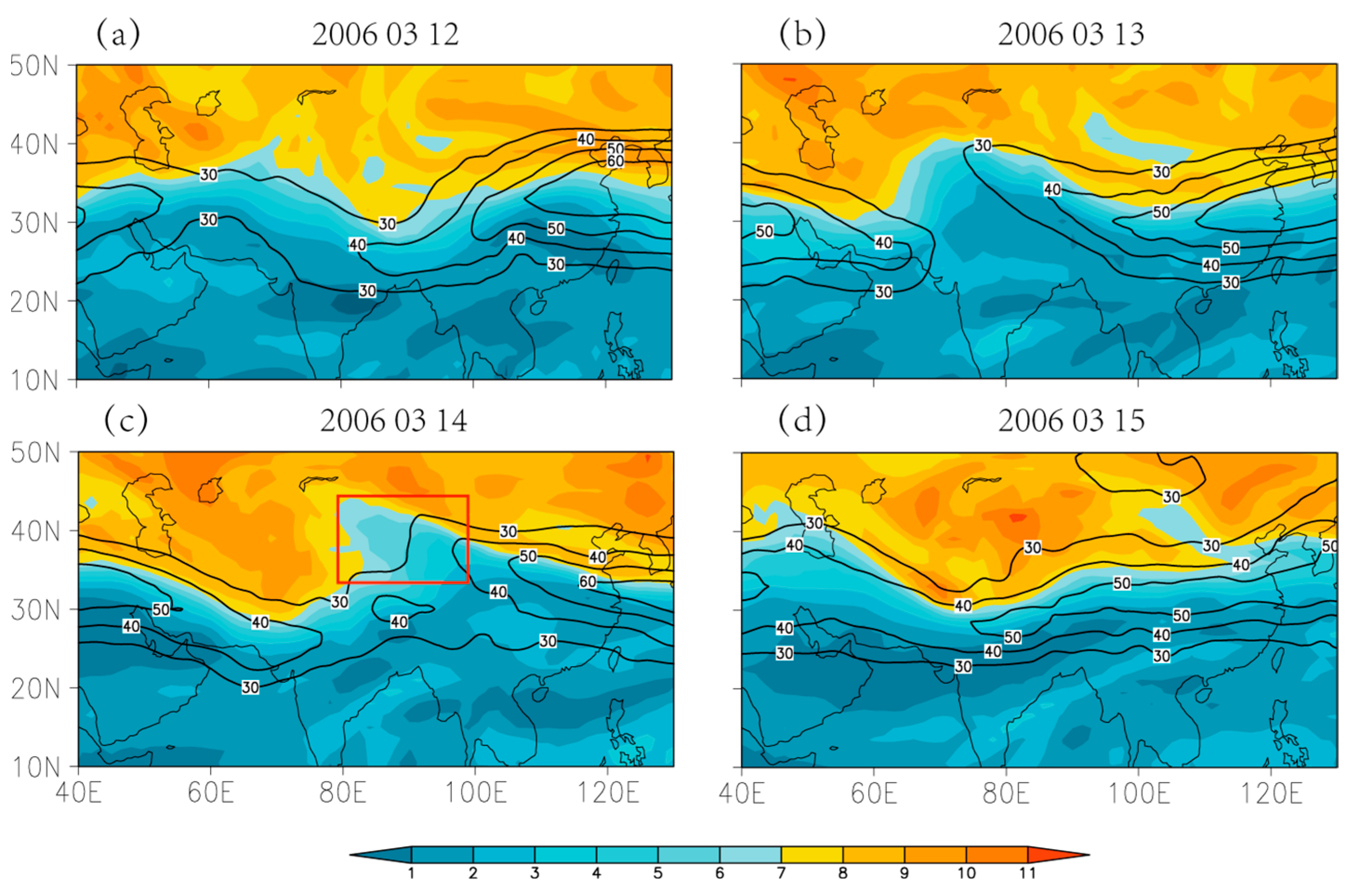
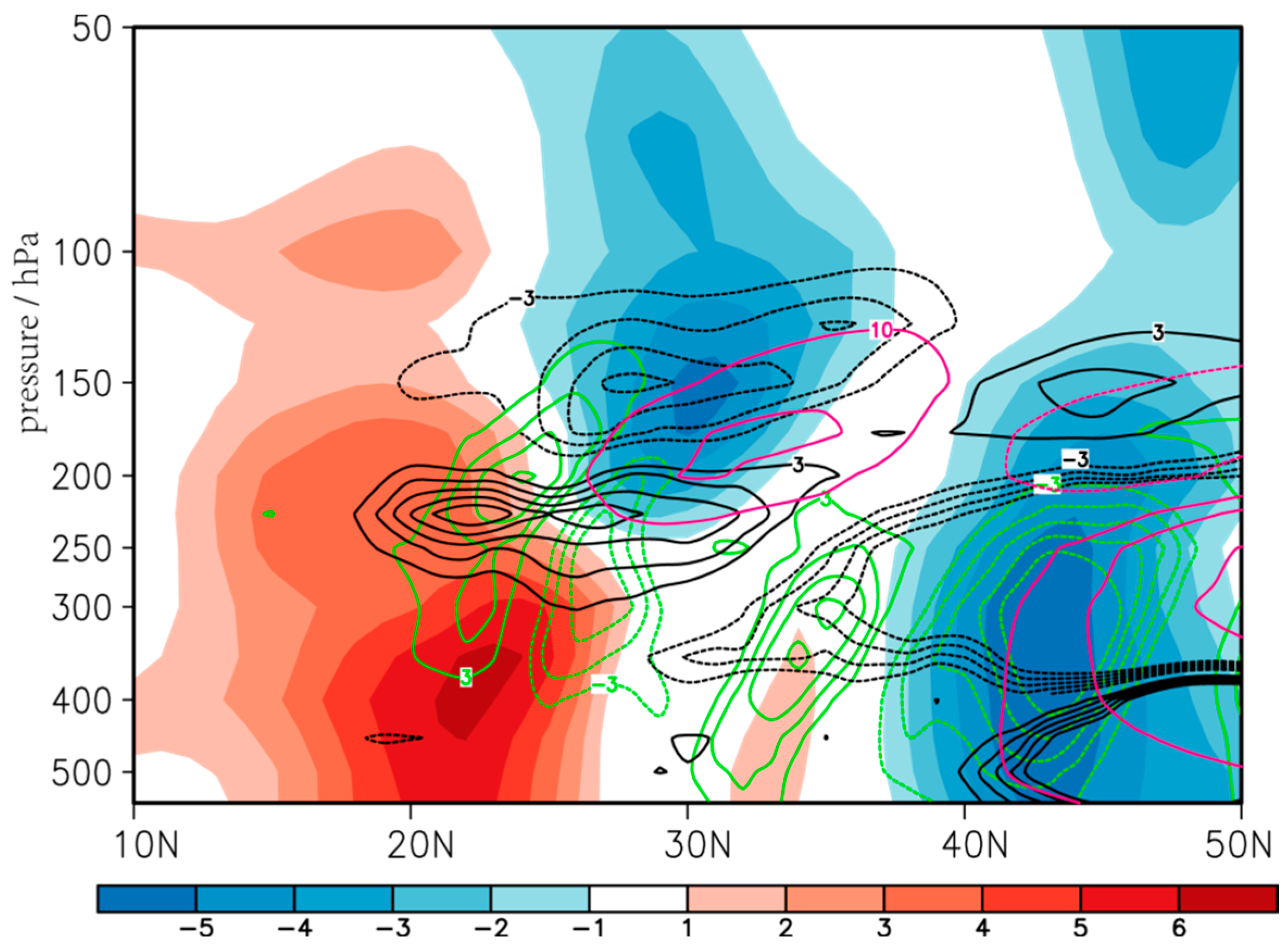
The evolution of potential vorticity (PV) on the 370-K isentropic surface can indicate the activity of Rossby waves near the subtropical high-level jet [44]. The amplitude of Rossby waves characterized by 5–8 PVU contours increased from 12 to 13 March 2006 (Figure 1). On 14 March, air mass with low PV extended to the northwest near 80°E and high-PV air mass occupied its south side, and thus there was a negative meridional gradient of PV instead of the conventional positive one. Hence, a cyclonic RWB event occurred. In the early stage of RWB, the subtropical high-level westerly jet slowed down and ended near 30°N on 13 March. The local Eliassen–Palm flux was used to diagnose the wave–mean flow interaction during 10–13 March (Figure 2), from which it can be seen there was a larger center of poleward transient eddy heat flux in the subtropical westerly jet region (pink contours >10 K⋅ms−1 in Figure 2), indicating that the baroclinic disturbance energy from the westerly jet promoted the development of a Rossby wave (also seen in Figure 1 during this period). On the other hand, the convergence of the vertical component of local Eliassen–Palm flux (black dotted contours in Figure 2, less than −5 m⋅s−1⋅day−1 near 30°N) decelerated the subtropical westerly jet (blue shaded area at 150 hPa in Figure 2, less than −5 m⋅s−1⋅day−1 near 30°N) according to the matched positions and values of those two anomalous centers. However, a corresponding relationship between the variation in the subtropical jet and the development of the Rossby wave was not evident in the eddy momentum flux (green contours in Figure 2). Hence, in the early stage, the eddy heat flux played an important role in the baroclinic development of RWB as mentioned by Simmons and Hoskins [45,46]. However, after the strongest stage of the disturbance, the occurrence of the RWB, the westerly jet can be strengthened by the energy feedback of the RWB, the barotropic conversion from eddy kinetic to zonal kinetic [45,46]. From 14 to 15 March, the subtropical westerly jet in Figure 1 was reconstructed.
3.2. Evolution of Thermal Structure and Ozone Concentration in the UTLS during the RWB
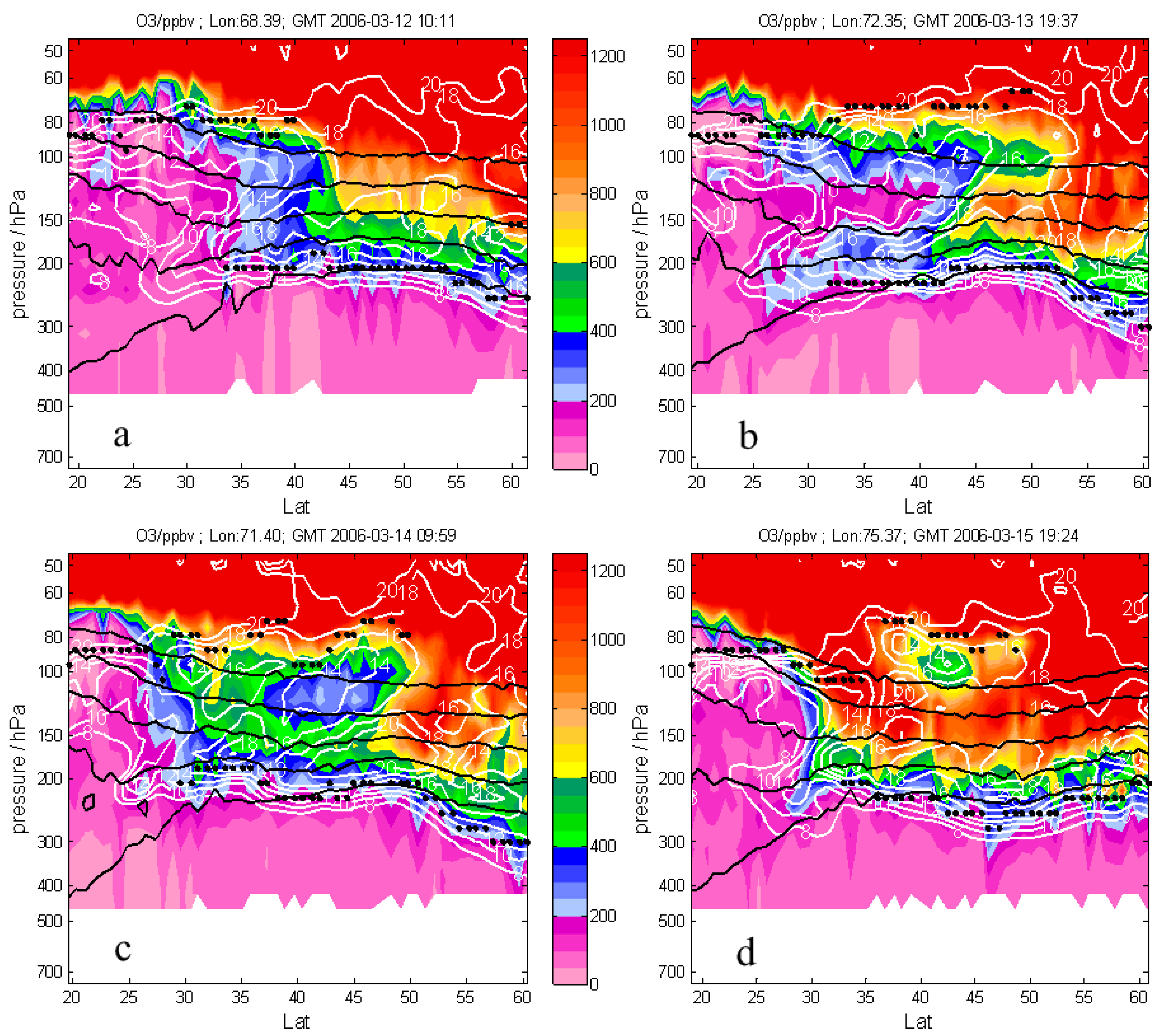
During the RWB in Asia in March 2006, a relatively complete STE process was detected by the HIRDLS ozone observations from the Aura satellite. On 12 March, there was a continuous high-level westerly jet greater than 30 m⋅s−1 on the 370-K isentropic surface (Figure 1a). The first and second thermodynamic tropopause (tropopause folding) were found above 35°–40°N on the vertical section along the satellite orbit near 70°E at the adjacent time, and the tropical tropopause layer (TTL) extended from the tropics to 35°–40°N where the discontinuity zones divided the tropospheric ozone-poor air with static stability less than 14 K⋅km−1 from the stratospheric ozone-rich air with static stability greater than 16 K⋅km−1 (Figure 3a). When the high-level westerly jet slowed on 13 March, the air mass with low PV invaded polewards along the gap of the jet greater than 30 m⋅s−1 over the Tibetan Plateau (Figure 1b). In the vertical section, the ozone-poor air with concentrations between 100 and 400 ppbv and static stability less than 14 K⋅km−1 intruded polewards from the TTL tropopause to 45°N at 150–100 hPa, and the second thermodynamic tropopause extended to 50°N. The meridional extent of the tropopause folding zone, indicated by the maximum gradients of ozone concentration and stability, extended polewards by 10° of latitude (Figure 3b). When the meridional gradients between the 6–8 PVU were reversed on 14 March near (80°E, 35°N) where a cyclonic wave-breaking event occurred, the low PV air with the value of 6–8 PVU invaded the Balkhash Lake region (Figure 1c) and the high-level jet that had broken off on the previous day was restored. In the vertical profile, the tropospheric air with ozone concentrations between 200 and 400 ppbv and static stability less than 14 K⋅km−1 had been transported polewards and separated from the TTL, and the front edge of the air mass reached 50°N in the mid-latitude stratosphere (Figure 3c). After being cut horizontally by the polar high-PV air on the south side, and after the tropospheric air had been surrounded by stratospheric air (ozone concentration greater than 400 ppbv and static stability greater than 16 K⋅km−1), a large-scale TST was completed (Figure 3c). On 15 March, the jet was further strengthened following reconstruction (Figure 1d) and the tropospheric characteristics of the air mass that entered the mid-latitude stratosphere (ozone concentration and stability) were weakening and were close to the environmental field including the ozone concentration and stability after turbulent exchange and mixing (Figure 3d).
3.3. Transport Pathway and Equivalent Mass of STE
The temporal and spatial resolution of the ERA-Interim dataset is limited. Although it could be used to analyze the dynamic mechanism of the large-scale RWB, a higher spatiotemporal resolution of data was required to accurately evaluate the STE transport caused by the RWB. Therefore, the WRF model, version 3.8.1, was used to conduct a high-resolution numerical simulation of the weather process, which particularly improved the vertical resolution of the UTLS, and a “sponge layer” with a thickness of 5 km was added to the upper boundary. The previous work of Shi et al. 2017 [20] proved the effectiveness of this scheme for structural simulation of the UTLS. This RWB case was also well simulated by the WRF model (figures omitted). When we detect whether an STE occurred for an air mass, its PV value is compared with the 7-PVU surface selected as the dynamic tropopause of the extratropical area in the Northern Hemisphere [31].
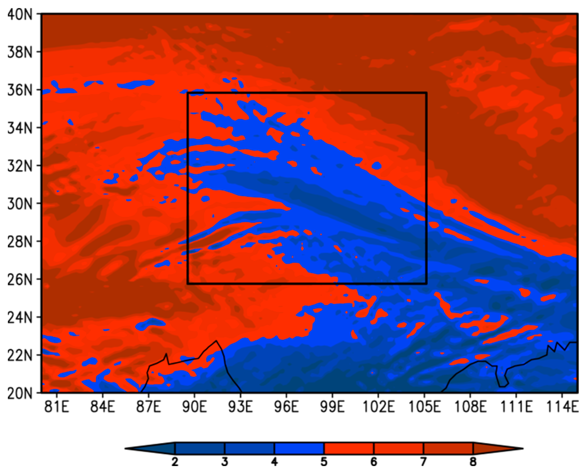
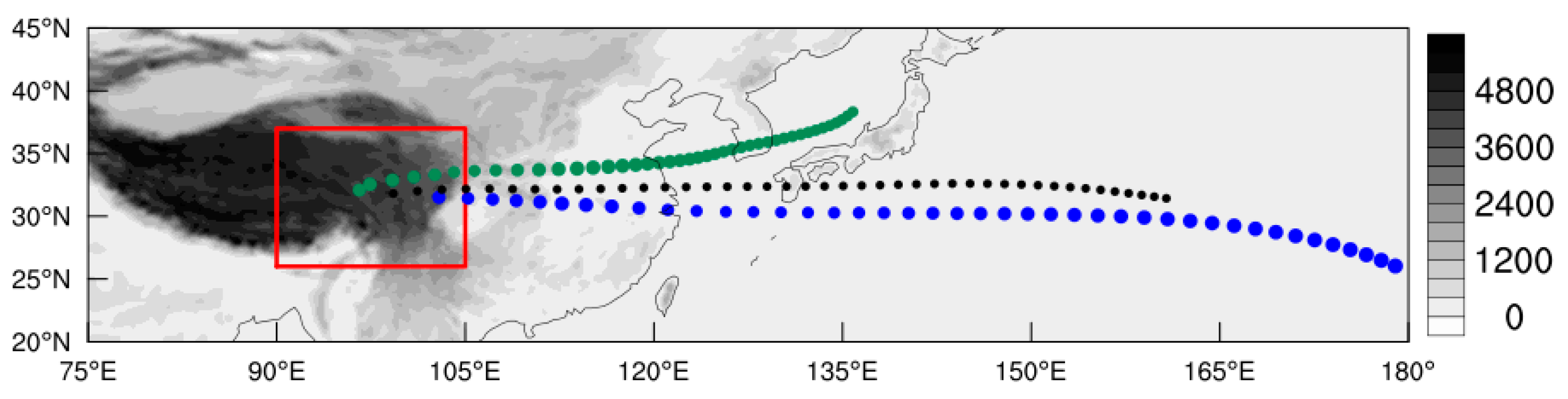
The WRF model recreated this RWB event well. The position where the RWB occurred in Figure 4 was situated between the locations in Figure 1c,d due to the differences of the time in those figures. The air mass between 13 km and 15 km near the tropopause in the black-framed area in Figure 4 was divided into 10,000 equal volumes of initial particles for trajectory analysis. According to reference [34], the average mass of each particle within a local spatial range was about 9.1 × 10¹⁰ kg. The main transport pathways along the southern or northern channels in the horizontal direction and along the upward or downward channels in the vertical direction for the particles were found, respectively, in Figure 5 and Figure 6, based on clustering analysis of the forward trajectory for 42 h. The particles in the northern branch (green dots in Figure 5) were initially located farther away from the core of the westerly jet than those in the southern branch (bule), which is also illustrated by the locations of the two white rectangles in Figure 7c,d. Due to the effect of cyclonic shearing to the north of the westerly jet core, the particles in the northern branch (green) broke away from the initial RWB region and migrated polewards. They were transported eastwards more slowly than those in the southern branch, spanning 40° of longitude compared with 85° of longitude.
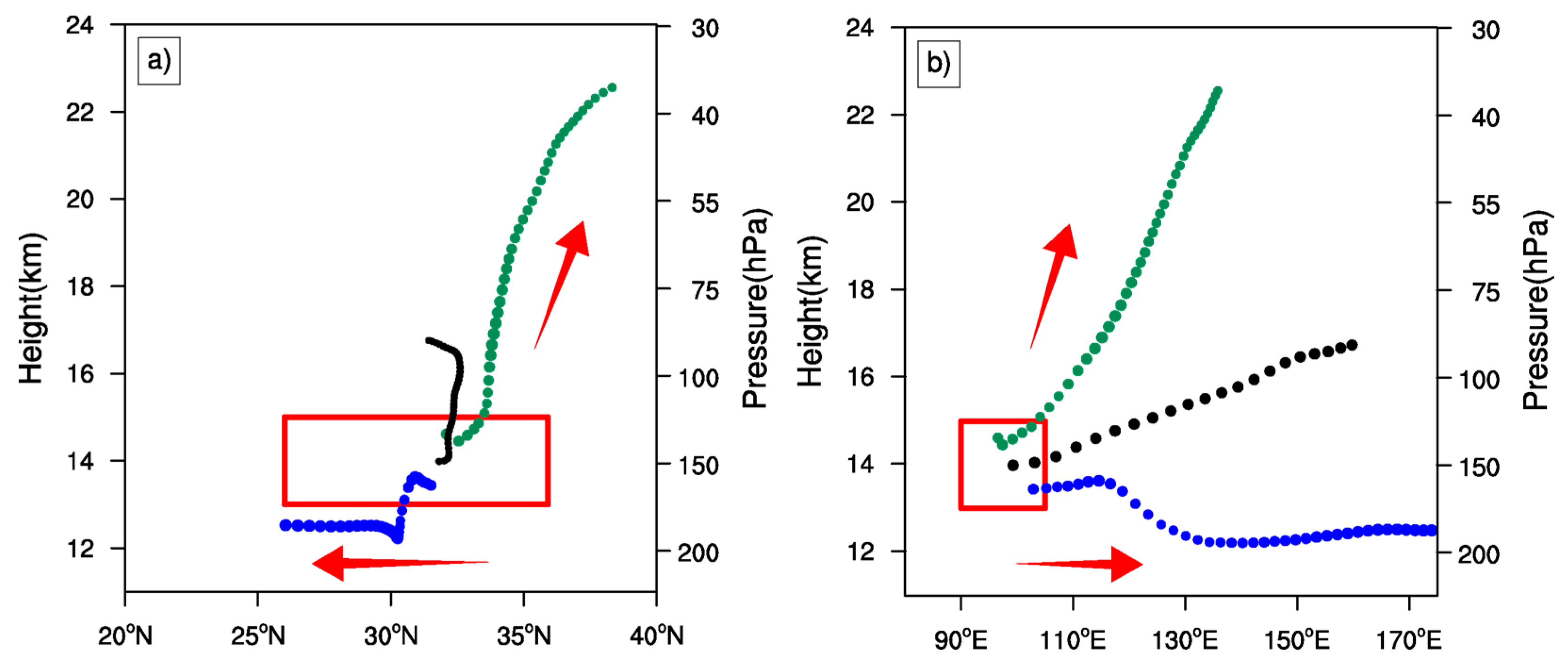
In the corresponding vertical profile, the particles in the northern branch (green dots in Figure 6) migrated from 32°N to 38°N and climbed up to 22 km from 14 km during a period of 42 h, which is also illustrated by the air masses with PV less than 7 PVU in the upper rectangle in Figure 7d. They were transported from the tropical troposphere to the extratropical stratosphere by the updrafts above the maximum convergence zone caused by the ageostrophic wind on the north side of the entrance of the downstream westerly jet core. Thus, the eastward migration of the particles (green dots in Figure 5 and Figure 6) with the convergence zone and the updrafts above on the north side of the westerly jet lasted 42 h (the northern rectangle in Figure 7c,d). After 42 h of forward transportation, 42.2% of the total 10,000 particles were transported from the tropical troposphere to the extratropical stratosphere. According to the average mass of each particle, 9.1 × 10¹⁰ kg estimated by volume, the mass of the TST was about 3.8 × 10¹⁴ kg. This result is comparable to a case study with a TST mass of 4.9 × 10¹⁴ kg in a tropopause folding event mentioned by Lamarque and Hess [47]. Other particles in the southern branch were transported eastwards to 110°E and then sank to 12 km in the tropical troposphere along the isentropic surface in the local upper frontal area (shown in Figure 6 and the lower rectangle in Figure 7d). These particles remained in the troposphere.
4. Conclusions and Discussion
Accompanying active and variable high-level jets in East Asia, RWB events often occur, which can play an important role in STE on synoptic scales. Based on satellite remote sensing data, numerical weather modeling, and Lagrangian trajectory analysis, we took an RWB event over the Tibetan Plateau in mid-March 2006 as an example to study the effects of RWB on the thermal structure and atmospheric composition near the tropopause and the features of the STE thereafter.
The increased eddy heat flux from the subtropical high-level westerly jet led to magnification of the amplitude of the Rossby wave, which was the dynamic background of the occurrence of the RWB event. The quasi-horizontal cyclonic shear of the Rossby wave cut the tropospheric air mass into the extratropical stratosphere, completing the stratosphere–troposphere mass exchange. During the RWB event, the tropopause folding zone extended polewards by 10° of latitude and the tropospheric air mass (ozone concentration between 100 and 400 ppbv; static stability less than 14 K⋅km−1) escaped from the TTL into the extratropical stratosphere through the tropopause folding zone. The particles migrated both eastwards and polewards in the horizontal direction, and upwards in the vertical direction along the TST pathway. Eventually, the total mass of the TST particles was about 3.8 × 10¹⁴ kg, accounting for 42.2% of the particles near the tropopause in the RWB event. The other particles remained in the troposphere. They moved eastwards faster in the westerly jet and flowed downslope along the isentropic surface in the downstream of the high-level front.
Although this study was based on an individual case analysis and may not be sufficiently representative, it is nevertheless valuable and reliable that this whole process was captured by the satellite remote sensing data. In future, we intend to identify more cases to reveal additional features of RWB and related STE in East Asia.
Author Contributions
Conceptualization, J.Z. and C.S.; Data curation, Formal analysis, J.Z., X.J. and C.S.; Investigation, Resources, Validation, Visualization, J.Z. and X.J.; Writing—original draft, J.Z. and C.S.; Writing—review and editing, C.S. and D.C. All authors have read and agreed to the published version of the manuscript.
Funding
This work is supported by the National Natural Science Foundation of China, under grants 41875048 and 91837311.
Data Availability Statement
The dataset from ERA-Interim for this study can be found at https://www.ecmwf.int/en/forecasts/dataset/ecmwf-reanalysis-interim, accessed on 20 September 2022. The Aura-HIRDLS satellite data can be found at https://disc.gsfc.nasa.gov/datasets?keywords=HIRDLS&page=1, accessed on 20 September 2022.
Acknowledgments
We thank NASA and ECMWF for the data provision. We acknowledge the high performance computing center of Nanjing University of Information Science and Technology for their support of this work. We are grateful to Dong Guo and Ziqian Zheng from Nanjing University of Information Science and Technology for their suggestions and help.
Conflicts of Interest
The authors declare no conflict of interest.
References
- Xia, Y.; Hu, Y.; Zhang, J.; Xie, F.; Tian, W. Record arctic ozone loss in spring 2020 is likely caused by north pacific warm sea surface temperature anomalies. Adv. Atmos. Sci. 2021, 38, 1723–1736. [Google Scholar] [CrossRef]
- Xie, F.; Tian, W.; Zhou, X.; Zhang, J.; Xia, Y.; Lu, J. Increase in lower stratospheric water vapor in the past 100 years related to tropical Atlantic warming. Geophys. Res. Lett. 2021, 47, e2020GL090539. [Google Scholar] [CrossRef]
- Yu, P.; Davis, S.M.; Toon, O.B.; Portmann, R.W.; Bardeen, C.G.; Barnes, J.E.; Telg, H.; Maloney, C.; Rosenlof, K.H. Persistent stratospheric warming due to 2019-20 Australian wildfire. Geophys. Res. Lett. 2021, 48, e2021GL092609. [Google Scholar] [CrossRef]
- Zhang, J.; Tian, W.; Xie, F.; Chipperfield, M.P.; Feng, W.; Son, S.W. Stratospheric ozone loss over the Eurasian continent induced by the polar vortex shift. Nat. Comm. 2018, 9, 206. [Google Scholar] [CrossRef] [Green Version]
- Zhou, X.; Chen, Q.; Li, Y.; Zhao, Y.; Lin, Y.; Jiang, Y. Impacts of the Indo-Pacific warm pool on lower stratospheric watervapor: Seasonality and hemispheric contrasts. J. Geophys. Res. Atmos. 2021, 126, e2020JD034363. [Google Scholar] [CrossRef]
- Chang, S.; Li, Y.; Shi, C.; Guo, D. Combined effects of the ENSO and the QBO on the ozone valley over the Tibetan Plateau. Remote Sens. 2022, 14, 4935. [Google Scholar] [CrossRef]
- Holton, J.; Haynes, P.; Mcintyre, M.; Douglass, A.; Rood, R.; Pfister, L. Stratosphere-troposphere exchange. Rev. Geophys. 1995, 33, 403–439. [Google Scholar] [CrossRef]
- Bian, J.; Li, D.; Bai, Z.; Li, Q.; Lyu, D.; Zhou, X. Transport of Asian surface pollutants to the global stratosphere from the Tibetan Plateau region during the Asian summer monsoon. Natl. Sci. Rev. 2020, 7, 516–533. [Google Scholar] [CrossRef] [Green Version]
- Chen, H.; Bian, J.; Lü, D. Advances and Prospects in the Study of Stratosphere-Troposphere Exchange. Chin. J. Atmos. Sci. 2006, 30, 813–820. (In Chinese) [Google Scholar]
- Wang, W.; Zuo, Q.; Wang, H.; Fan, W.; Bian, J.; Peng, Y.; Li, X. The structure of O3/H2O mixing relationships in the tropopause transition layer in middle and high latitudes of the Northern Hemisphere. Chin. J. Geophys. 2010, 53, 2805–2816. [Google Scholar]
- Pan, L.L.; Bowman, K.P.; Atlas, E.L.; Wofsy, S.; Zhang, F.; Bresch, J.; Ridley, B.; Pittman, J.; Homeyer, C.; Romashkin, P.; et al. The stratosphere–troposphere analyses of regional transport 2008 Experiment. Bul. Am. Meteorol. Soc. 2010, 91, 327–342. [Google Scholar] [CrossRef]
- Tian, H.; Tian, W.; Luo, J.; Zhang, J.; Zhang, M. Climatology of cross-tropopause mass exchange over the Tibetan Plateau and its surroundings. Inter. J. Clim. 2017, 37, 3999–4014. [Google Scholar] [CrossRef]
- Yu, P.; Rosenlof, K.H.; Liu, S.; Telg, H.; Bai, X.; Portmann, R.W.; Rollins, A.W.; Pan, L.L.; Toon, O.B.; Bian, J.; et al. Efficient transport of tropospheric aerosol into the stratosphere via the Asian summer monsoon anticyclone. Proc. Natl. Acad. Sci. USA 2017, 114, 6972–6977. [Google Scholar] [CrossRef] [PubMed] [Green Version]
- Li, D.; Bian, J. Case analyses and numerical simulation of transport process caused by convection associated with northeast cold vortex. Chin. J. Geophys. 2018, 61, 3607–3616. [Google Scholar]
- Shi, C.; Guo, D.; Li, H.; Zheng, B.; Liu, R. Stratosphere-troposphere exchange corresponding to a deep convection in warm sector and abnormal subtropical front induced by a cutoff low over East Asia. Chin. J. Geophys. 2014, 57, 1–10. [Google Scholar]
- Chen, Q.; Gao, G.; Li, Y.; Cai, H.; Zhou, X.; Wang, Z. Main detrainment height of deep convection systems over the Tibetan plateau and its southern slope. Adv. Atmos. Sci. 2019, 36, 1078–1088. [Google Scholar] [CrossRef]
- Yan, Q.; Luo, J.; Shang, L.; Li, Y.; Suo, C.; Cui, Q. A case study of stratosphere -troposphere exchange during meiyu season. J. Arid. Meteorol. 2017, 35, 12–22. (In Chinese) [Google Scholar]
- Chen, B.; Xu, X.; Yang, S.; Zhao, T. Climatological perspectives of air transport from atmospheric boundary layer to tropopause layer over Asian monsoon regions during boreal summer inferred from Lagrangian approach. Atmos. Chem. Phys. 2012, 13, 5827–5839. [Google Scholar] [CrossRef] [Green Version]
- Chen, D.; Zhou, T.; Ma, L.; Shi, C.; Guo, D.; Chen, L. Statistical analysis of the spatiotemporal distribution of ozone induced by cut-off lows in the upper troposphere and lower stratosphere over northeast Asia. Atmosphere 2019, 10, 696. [Google Scholar] [CrossRef] [Green Version]
- Shi, C.; Cai, W.; Guo, D. Composition and thermal structure of the upper troposphere and lower stratosphere in a penetrating mesoscale convective complex determined by satellite observations and model simulations. Adv. Meteorol. 2017, 2017, 6404796. [Google Scholar] [CrossRef] [Green Version]
- Wei, D.; Tian, W.; Chen, Z.; Zhang, J. Upward transport of air mass during a generation of orographic waves in the UTLS over the Tibetan Plateau. Chin. J. Geophys. 2016, 59, 791–802. [Google Scholar]
- Cooper, O.; Foster, C.; Parrish, D.; Dunlea, E.; Hübler, G.; Fehsenfeld, F.; Holloway, J.; Oltmans, S.; Johnson, B.; Wimmers, A.; et al. On the life cycle of a stratospheric intrusion and its dispersion into polluted warm conveyor belts. J. Geophys. Res. Atmos. 2004, 109, D23S09. [Google Scholar] [CrossRef]
- Li, D.; Bian, J.; Fan, Q. A deep stratospheric intrusion associated with an intense cut-off low event over East Asia. Sci. Chin. Earth. Sci. 2015, 58, 116–128. [Google Scholar] [CrossRef]
- Pan, L.L.; Randel, W.J.; Gille, J.C.; Hall, W.; Nardi, B.; Massie, S.; Yudin, V.; Khosravi, R.; Konopka, P.; Tarasick, D. Tropospheric intrusions associated with the secondary tropopause. J. Geophys. Res. Atmos. 2009, 114, D10302. [Google Scholar] [CrossRef] [Green Version]
- Hofmann, C.; Kerkweg, A.; Hoor, P.; Jöckel, P. Stratosphere-troposphere exchange in the vicinity of a tropopause fold. Atmos. Chem. Phys. 2016, 16, 1–26. [Google Scholar]
- Homeyer, C.R.; Bowman, K.P. Rossby Wave Breaking and Transport between the Tropics and Extratropics above the Subtropical Jet. J. Atmos. Sci. 2013, 70, 607–626. [Google Scholar] [CrossRef] [Green Version]
- Postel, G.A. A climatology of Rossby wave breaking along the subtropical tropopause. J. Atmos. Sci. 1999, 56, 3605–3611. [Google Scholar] [CrossRef]
- Wernli, H.; Sprenger, M. Identification and ERA-15 Climatology of Potential Vorticity Streamers and Cutoffs near the Extratropical Tropopause. J. Atmos. Sci. 2007, 64, 1569–1586. [Google Scholar] [CrossRef]
- Waugh, D.W.; Polvani, L.M. Climatology of intrusions into the tropical upper troposphere. Geophys. Res. Lett. 2000, 27, 3857–3860. [Google Scholar] [CrossRef] [Green Version]
- Manney, G.L.; Hegglin, M.I.; Daffer, W.H.; Schwartz, M.; Santee, M.; Pawson, S. Climatology of Upper Tropospheric–Lower Stratospheric (UTLS) Jets and Tropopauses in MERRA. J. Clim. 2014, 27, 3248–3271. [Google Scholar] [CrossRef]
- Homeyer, C.; Bowman, K.; Pan, L.; Atlas, E.; Gao, R.; Campos, T. Dynamical and chemical characteristics of tropospheric intrusions observed during START08. J. Geophys. Res. Atmos. 2011, 116, D06111. [Google Scholar] [CrossRef] [Green Version]
- Kunz, A.; Sprenger, M.; Wernli, H. Climatology of potential vorticity streamers and associated isentropic transport pathways across PV gradient barriers. J. Geophys. Res. Atmos. 2015, 120, 3802–3821. [Google Scholar] [CrossRef]
- Dee, D.P.; Uppala, S.M.; Simmons, A.J.; Berrisford, P.; Poli, P.; Kobayashi, S. The ERA-Interim reanalysis: Configuration and performance of the data assimilation system. Quart. J. Roy. Meteor. Soc. 2011, 137, 553–597. [Google Scholar] [CrossRef]
- Skerlak, B.; Sprenger, M.; Wernli, H. A global climatology of stratosphere –troposphere exchange using the ERA-Interim data set from 1979 to 2011. Atmos. Chem. Phys. 2014, 14, 913–937. [Google Scholar] [CrossRef] [Green Version]
- Gille, J.; Barnett, J.; Arter, P.; Barker, M.; Bernath, P.; Boone, C. High Resolution Dynamics Limb Sounder: Experiment overview, recovery, and validation of initial temperature data. J. Geophys. Res. Atmos. 2008, 113, D16S43. [Google Scholar] [CrossRef] [Green Version]
- Thorncroft, C.D.; Hoskins, B.J.; Mcintyre, M.E. Two paradigms of baroclinic -wave life-cycle behaviour. Quart. J. Roy. Meteor. Soc. 1993, 119, 17–55. [Google Scholar] [CrossRef]
- Trenberth, K.E. An assessment of the impact of transient eddies on the zonal flow during a blocking episode using localized Eliassen-Palm flux diagnostics. J. Atmos. Sci. 1986, 43, 2070–2087. [Google Scholar] [CrossRef]
- Grell, G.A.; Freitas, S.R. A scale and aerosol aware stochastic convective parameterization for weather and air quality modeling. Atmos. Chem. Phys. 2014, 14, 5233–5250. [Google Scholar] [CrossRef] [Green Version]
- Mlawer, E.J.; Taubman, S.J.; Brown, P.D. Radiative transfer for inhomogeneous atmosphere: RRTM, a validated correlated-k model for the longwave. J. Geophys Res. 1997, 102, 16663–16682. [Google Scholar] [CrossRef] [Green Version]
- Dudhia, J. Numerical study of convection observed during the winter Monsoon experiment using a mesoscale two-dimensional model. J. Atmos. Sci. 1989, 46, 3077–3107. [Google Scholar] [CrossRef]
- Hong, S.Y. A new vertical diffusion package with an explicit treatment of entrainment processes. Mon. Weather. Rev. 2006, 134, 2318. [Google Scholar] [CrossRef] [Green Version]
- Mansell, E.R.; Ziegler, C.L.; Bruning, E.C. Simulated Electrification of a Small Thunderstorm with Two-Moment Bulk Microphysics. J. Atmos. Sci. 2020, 67, 171. [Google Scholar] [CrossRef]
- Stohl, A.; Forster, C.; Frank, A.; Seibert, P.; Wotawa, G. Technical note: The Lagrangian particle dispersion model FLEXPART version 6.2. Atmos. Chem. Phys. 2005, 5, 2461–2474. [Google Scholar] [CrossRef] [Green Version]
- Kunz, A.; Konopka, P.; Müller, R.; Pan, L. Dynamical tropopause based on isentropic potential vorticity gradients. J. Geophys. Res. Atmos. 2011, 116, D01110. [Google Scholar] [CrossRef] [Green Version]
- Simmons, A.J.; Hoskins, B.J. Barotropic influences on the growth and decay of nonlinear baroclinic waves. J. Atmos. Sci. 1980, 37, 1679–1684. [Google Scholar] [CrossRef]
- Simmons, A.J.; Hoskins, B.J. The Life Cycles of Some Nonlinear Baroclinic Waves. J. Atmos. Sci. 1978, 35, 414–432. [Google Scholar] [CrossRef]
- Lamarque, J.F.; Hess, P.G. Cross-tropopause mass exchange and potential vorticity budget in a simulated tropopause folding. J. Atmos. Sci. 1994, 51, 2246–2269. [Google Scholar] [CrossRef]
Figure 1.
Diurnal evolution of the PV (shaded; unit: PVU, 1 PVU = 10−6 m2⋅s−1⋅K⋅kg−1) and zonal wind (contours; unit: m⋅s−1) on the 370-K isentropic surface at (a) 1200 UTC 12 March 2006, (b) 1200 UTC 13 March 2006, (c) 1200 UTC 14 March 2006 and (d) 1200 UTC 15 March 2006.
Figure 1.
Diurnal evolution of the PV (shaded; unit: PVU, 1 PVU = 10−6 m2⋅s−1⋅K⋅kg−1) and zonal wind (contours; unit: m⋅s−1) on the 370-K isentropic surface at (a) 1200 UTC 12 March 2006, (b) 1200 UTC 13 March 2006, (c) 1200 UTC 14 March 2006 and (d) 1200 UTC 15 March 2006.

Figure 2.
Zonal mean temporal variation of zonal wind (shaded; unit: m⋅s−1⋅day−1), eddy heat flux (pink contours; interval: 10 K⋅m⋅s−1), and local Eliassen–Palm flux divergence (green contours representing the horizontal component and black contours representing the vertical component; interval: 2 m⋅s−1⋅day−1) between 50°E and 70°E from 10 to 13 March 2006.

Figure 3.
Vertical sections near the RWB along the satellite track on (a) 12 March 2006, (b) 13 March 2006, (c) 14 March 2006 and (d) 15 March 2006 of the ozone concentrations from HIRDLS (shaded; unit: ppbv), potential temperature (black contours for 330 K, 350 K, 370 K, 390 K, and 410 K) and its vertical gradients (white contours; unit: K km−1). The black spots represent the positions of the tropopause defined by the temperature lapse rate.

Figure 4.
Mean PV (shaded; unit: PVU) of WRF outputs between the 100 hPa and 200 hPa isobaric surfaces at 0600 UTC 15 March 2006. The initial positions of the released particles are located in the black frame.
Figure 4.
Mean PV (shaded; unit: PVU) of WRF outputs between the 100 hPa and 200 hPa isobaric surfaces at 0600 UTC 15 March 2006. The initial positions of the released particles are located in the black frame.

Figure 5.
Horizontal forward trajectories of the released particles determined by cluster analysis from 0600 UTC 15 March 2006 to 0000 UTC 17 March 2006. Green dots and blue dots represent the two cluster analysis trajectories. Black dots represent the trajectory of the total mass center. The terrain height (unit: m) is shaded.

Figure 6.
As in Figure 5 but along (a) a meridional cross section and (b) a zonal cross section.
Figure 6.
As in Figure 5 but along (a) a meridional cross section and (b) a zonal cross section.

Figure 7.
Vertical sections along (a) 80°E, (b) 90°E, (c) 100°E and (d) 110°E, from 13 to 16 March 2006, respectively, of PV (shading; unit: PVU), zonal wind (black contours; unit: m s−1), and potential temperature (grey contours; unit: K). The white rectangles illustrate the two clustering locations of air particles.

Disclaimer/Publisher’s Note: The statements, opinions and data contained in all publications are solely those of the individual author(s) and contributor(s) and not of MDPI and/or the editor(s). MDPI and/or the editor(s) disclaim responsibility for any injury to people or property resulting from any ideas, methods, instructions or products referred to in the content. |
© 2022 by the authors. Licensee MDPI, Basel, Switzerland. This article is an open access article distributed under the terms and conditions of the Creative Commons Attribution (CC BY) license (https://creativecommons.org/licenses/by/4.0/).
Share and Cite
MDPI and ACS Style
Zhu, J.; Jin, X.; Shi, C.; Chen, D. The Troposphere-to-Stratosphere Transport Caused by a Rossby Wave Breaking Event over the Tibetan Plateau in Mid-March 2006. Remote Sens. 2023, 15, 155. https://doi.org/10.3390/rs15010155
AMA Style
Zhu J, Jin X, Shi C, Chen D. The Troposphere-to-Stratosphere Transport Caused by a Rossby Wave Breaking Event over the Tibetan Plateau in Mid-March 2006. Remote Sensing. 2023; 15(1):155. https://doi.org/10.3390/rs15010155
Chicago/Turabian StyleZhu, Jinyao, Xin Jin, Chunhua Shi, and Dan Chen. 2023. "The Troposphere-to-Stratosphere Transport Caused by a Rossby Wave Breaking Event over the Tibetan Plateau in Mid-March 2006" Remote Sensing 15, no. 1: 155. https://doi.org/10.3390/rs15010155
Note that from the first issue of 2016, this journal uses article numbers instead of page numbers. See further details here.