

Assessment of the Impact of Rubber Plantation Expansion on Regional Carbon Storage Based on Time Series Remote Sensing and the InVEST Model


1
State Key Laboratory of Resources and Environmental Information System, Institute of Geographic Sciences and Natural Resources Research, Chinese Academy of Sciences, Beijing 100101, China
2
CAS Engineering Laboratory for Yellow River Delta Modern Agriculture, Institute of Geographic Sciences and Natural Resources Research, Chinese Academy of Sciences, Beijing 100101, China
*
Author to whom correspondence should be addressed.
†
These authors contributed equally to this work.
Remote Sens. 2022, 14(24), 6234; https://doi.org/10.3390/rs14246234
Submission received: 15 October 2022
/
Revised: 26 November 2022
/
Accepted: 5 December 2022
/
Published: 9 December 2022
(This article belongs to the Special Issue Monitoring Forest Carbon Sequestration with Remote Sensing)
Abstract
:Rubber plantations in southeast Asia have grown at an unprecedented rate in recent decades, leading to drastic changes in regional carbon storage. To this end, this study proposes a systematic approach for quantitatively estimating and assessing the impact of rubber expansions on regional carbon storage. First, using Sentinel-1 and Sentinel-2 satellite data, the distributions of forest and rubber, respectively, were extracted. Then, based on the Landsat time series (1999–2019) remote sensing data, the stand age estimation of rubber plantations was studied with the improved shapelet algorithm. On this basis, the Ecosystem Services and Tradeoffs model (InVEST) was applied to assess the regional carbon density and storage. Finally, by setting up two scenarios of actual planting and hypothetical non-planting of rubber forests, the impact of the carbon storage under these two scenarios was explored. The results of the study showed the following: (1) The area of rubber was 1.28 × 10⁵ ha in 2019, mainly distributed at an elevation of 200–400 m (accounting for 78.47% of the total of rubber). (2) The average age of rubber stands was 13.85 years, and the total newly established rubber plantations were converted from cropland and natural forests, accounting for 54.81% and 45.19%, respectively. (3) With the expansion of rubber plantations, the carbon density increased from only 2.25 Mg·C/ha in 1999 to more than 15 Mg·C/ha in 2018. Among them, the carbon sequestration increased dramatically when the cropland was replaced by rubber, while deforestation and replacement of natural forests will cause a significant decrease. (4) The difference between the actual and the hypothetical carbon storage reached −0.15 million tons in 2018, which means that the expansion of rubber led to a decline in carbon storage in our study area. These research findings can provide a theoretical basis and practical application for sustainable regional rubber forest plantation and management, carbon balance maintenance, and climate change stabilization.
1. Introduction
Carbon sequestration in terrestrial ecosystems is critical to the effects of carbon dioxide (CO2)-driven global climate change [1,2,3]. As an important part of the terrestrial ecosystem and the largest carbon pool, the annual carbon sequestration of forests accounts for about two-thirds of the entire terrestrial ecosystem, playing an important role in reducing the rise in atmospheric CO2 concentration and stabilizing global climate change [4,5]. Therefore, the study of carbon storage in the forest ecosystem is a hotspot of carbon neutralization research and focus of current global climate change research [6]. However, today’s research is mainly focused on the carbon stock of primary natural forests, and relatively less research has been conducted on the carbon sink balance of the artificial forests, which accounts for seven percent of the world’s overall forest area [5,7]. Therefore, it is necessary to study the change in carbon storage in key plantation forest types.
Rubber forests, as the second largest tropical plantation ecosystem after oil palm [8], are planted for their large economic value, and they have a strong carbon sequestration capacity that plays an important role in the economic development and ecosystem service value [9,10]. Southeast Asia is the world’s major natural rubber growing region because of its suitable climate and growing conditions, accounting for more than 80% of the global natural rubber forest plantation area [11,12]. With the rapid development of economic globalization, the importance of rubber products in the national economy is increasing, the rigid demand for natural rubber is growing, and the planting area of rubber is expanding [13,14]. According to the statistics, the area planted with rubber forests in Thailand increased by nearly 800% from about 400,000 ha in 1961 to more than 3 million ha in 2017 [15]. However, most rubber forests are planted at the expense of the primary tropical rainforests or secondary forests, which inevitably leads to a certain loss of carbon sinks [7,16,17]. In addition, the deforestation of the tropical rainforest caused by rubber forest plantations will inevitably lead to the continuous reduction in the tropical rainforest-based biological habitat, the gradual reduction of soil and water conservation capacity, regional environmental degradation, and serious damage to biodiversity and the ecological environment [18,19,20,21]. Therefore, it is of great significance to understand the quantitative impact of rubber forests on carbon storage for the rational development of rubber plantations, the protection of forest ecosystems, the maintenance of the carbon sink balance, and the stability of climate change.
The age information of rubber is the key parameter of carbon storage assessment and can improve the accuracy of rubber carbon storage estimation [7]. Traditional rubber forest age monitoring is mainly based on the ground survey of sampling theory, which is time-consuming, labor-intensive, not comprehensive, and may be less accurate for regional estimations [10,22,23,24,25]. Access to information about the age of rubber on each plantation is even more difficult in areas where rubber plantations are small, fragmented, flexible cropping systems, with high variability in planting status, and which are mainly established and managed by smallholders, e.g., in Thailand, where an estimated 90% of rubber is produced by smallholders [16]. With the development of earth observation technology, remote sensing, which is macro, rapid, dynamic, and rich in information acquisition capacity, has been used to map rubber plantations and become an effective means of extracting age information from rubber in recent years [10,22,26,27].
The methods for age identification of rubber forests using remote sensing can commonly be divided into four main categories: post-classification comparison (PCC) [28], threshold method [29,30], regression method [10,23,25], and trajectory analysis method [14,31]. The PCC method first extracts rubber results at different times and then analyzes the classifications by superposition and statistics to obtain the age of rubber forests [32]. However, images of key phenological periods are often not available owing to the frequent cloud cover in tropical regions. In most cases, because of the extreme spectral similarity between rubber and natural forests, classification errors may result in high uncertainty of the rubber forest change detection and age extraction [15,33,34]. The threshold method sets certain thresholds to extract change information according to the pattern of vegetation indices (VIs) over time [29,30]. However, the threshold value of the VIs may fluctuate owing to the different rubber species, phenological period, or geographical environment, and setting a specific threshold value may cause some uncertainty in the extraction of the age information [18]. The regression method estimates stand age by establishing a regression model between spectral bands, vegetation indices or backscatter coefficients of synthetic aperture radar (SAR) images, and stand age of rubber [23,25]. However, because the coefficients saturate after a certain stand age, the reflectance values of young and open canopy stands are likely to be influenced by ground cover crops, and the regression method may seriously overestimate young stands and underestimate old stands. Compared with the previous three methods, the trajectory analysis method is considered more robust to inherent noise in the data (e.g., interannual variation) and has become an important research hotspot for the extraction of land-related type change information [14,22]. The trajectory analysis method also contains many algorithms, such as Landtrendr [35] and shapelet [14] to extract the age of rubber forests. However, these algorithms require a large amount of storage and incur high computational costs. Fortunately, with the free sharing of the Google Earth Engine (GEE) remote sensing cloud computing platform [36,37], which provides fast processing and analysis of massive remote sensing data, there is strong technical support for the real-time processing of large-scale and long-term remote sensing data. Therefore, combined with long time series satellite remote sensing data and GEE cloud platform, the relevant algorithms of the trajectory analysis method can be developed to achieve the identification of rubber tree age and pre-conversion land cover in large areas.
For the carbon storage of rubber forests, traditional estimation methods, such as the stockpile method, biomass method, and box method for the field monitoring of carbon storage, are clear and explicit, easy to apply, and more widely used [38,39]. However, because of the inconsistency of measurement methods, sampling locations, and study scales, the results vary and cannot accurately reflect the changes in carbon storage over long periods of time and large scales. With the development of information technology, remote sensing biomass estimation transformation methods and remote sensing-driven model simulation methods have emerged [40,41,42,43]. However, these methods either need extensive ground survey data to support them or have problems with complicated model-driven data [40,44]. With the carbon storage model of the Integrated Valuation of Ecosystem Services and Tradeoffs model (InVEST) proposal [45,46], more and more scholars at home and abroad have started to use the carbon storage module [47] of the InVEST model to estimate regional carbon storage in terrestrial ecosystems [48,49,50]. Compared with the traditional carbon storage estimation methods, the carbon module of InVEST has the advantages of simple and easy access to driving data (e.g., types and carbon densities of the land use/land cover (LULC)), simple operation, fast running speed, and strong visibility of output results. It can realize mapping of spatial distribution and dynamic changes of carbon storage [41] and reflect the relationship between land-use change and carbon storage under different scenarios [9]. However, existing studies [50,51,52] generally focus on the effects of all types of LULC on total carbon stock, and relatively little research has been conducted on the effects of single land-use types (e.g., rubber forests) on total carbon storage, which may be important for forest carbon neutralization [19]. In addition, the existing studies [50,51,52] on carbon storage estimation in rubber forests are basically converted from biomass by assuming a constant value or approximating the multi-year average rate, which will inevitably lead to large uncertainties in the actual carbon storage simulations. Therefore, using the age data of rubber, the InVEST model can improve the temporal dynamic evolution of carbon storage in the rubber forest, improving the accuracy of carbon storage simulation to a certain extent.
Thus, this study takes northeast Thailand, where rubber plantations are expanding rapidly, as an example to assess the impact of spatial and temporal changes in rubber planting on carbon storage over the past two decades. The objectives of this study are (1) to develop an algorithm for mapping the stand ages of rubber plantations and identify the land-cover types prior to rubber plantation conversion; (2) to analyze the spatial and temporal patterns of carbon sequestration under the expansion of rubber plantations using the InVEST model; and (3) to explore the differences in carbon sequestration processes between planted and non-rubber-planted conditions.
2. Materials and Methods
2.1. Study Area
The province of Loei is located in northeast Thailand with elevation ranging from 100 to 1798 m (Figure 1). This area features a humid subtropical monsoon climate with two main seasons: a rainy season from May to October and a dry season from November to April. The southwest monsoon brings abundant precipitation to the study area, and the heavy rainfall is concentrated in August or September [36].
Traditionally, northeastern Thailand has been an important cultivation area with fewer rubber plantations. Encouraged by an active government policy for rubber plantations since 2003, the rubber plantation area has expanded rapidly in northeastern Thailand [33]. As a result, rapid land use and land cover change has taken place in most of its territory. Many patches of natural forest and cropland have been encroached on by rubber plantations, which can nowadays be found all over Loei from the highland areas down to the low-lying plains [16]. Therefore, it is of great practical value to assess the rubber plantations impact on carbon storage in the study area for the development of sustainable rubber plantations and forest conservation.
2.2. Data
2.2.1. Remote Sensing Data and Preprocessing
- Sentinel-1 data and preprocessing
A total of 170 scenes of Sentinel-1A and Sentinel-1B interferometric wide swath ground range detected (GRD) images of 2019 from the GEE platform [53] were used to generate a forest map (including rubber plantations). The Sentinel-1 data in GEE were pre-processed with the Sentinel-1 Toolbox using orbit metadata update, GRD border noise removal, thermal noise removal, radiometric calibration, and terrain correction [36]. The final terrain-corrected digital number (DN) values were converted to decibels (dB) in each pixel via log scaling 10log10(DN). A Refined Lee filter was applied to de-speckle the images. Two additional indices, including (1) the ratio of the dual polarization of vertical transmit and vertical receive (VV) to vertical transmit and horizontal receive (VH) dB data (Ratio = dBVV/dBVH), and (2) the difference between VV and VH dB data (Difference = dBVV − dBVH), were also calculated for each image. The annual mean value indicators (i.e., VV_mean, VH_mean, Ratio_mean, and Difference_mean) were generated for forest mapping, since the mean images can reduce the geometric and radiometric distortion of Sentinel-1 SAR images [54].
- Sentinel-2 data and preprocessing
Four Sentinel-2 Level 1C data (tile: 47QQU, 47QQV, 47QRU, 47QRV) were downloaded from the European Space Agency’s (ESA) Copernicus Scihub [55]. The acquired Sentinel-2 data were obtained on 23 March 2019. Radiometric and geometric corrections were conducted to acquire top-of-atmosphere (TOA) reflectance. We conducted atmospheric correction and obtained surface reflectance using ESA’s Sen2Cor in Sentinel Application Platform (SNAP) 7.0 software [56]. The spatial resolution of Sentinel-2 data varies from 10 to 60 m. Bands of 1, 9, and 10 were excluded from the dataset owing to their sensitivity to aerosol and clouds and their spatial resolution (60 m). Then, the images were resampled at 10 m using a bilinear method [56]. In all, 33 spectral indices were calculated based on the surface reflectance [57], including the Normalized Difference Vegetation Index (NDVI) [58], the Enhanced Vegetation Index (EVI) [59], and the Red-edge Normalized Difference Vegetation Index 1 (NDVIre1) [60]. A full list detailing all spectral indices can be found in the Supplementary Material (Table S1). Eight textural features were derived using a gray-level co-occurrence matrix (GLCM) [61], including mean (MEAN), variance (VAR), homogeneity (HOM), contrast (CON), dissimilarity (DIS), entropy (ENT), angular second moment (ASM), and correlation (COR).
- Landsat data and preprocessing
We obtained cloud-free Landsat thematic mapper (TM), enhanced thematic mapper plus (ETM+), operational land imager (OLI) images spanning 1999–2019 with one image per year for the study region (worldwide reference system 2 (WRS-2) path/row = 129/48) (Table 1). To reduce the errors and uncertainties caused by different months and clouds/rain, cloud-free satellite images were only collected for the dry season (mid-October to mid-May of the following year). The Landsat data were downloaded from the USGS [62]. Radiometric calibration, atmospheric correction, and geometric correction were conducted for each image. All acquired data were georeferenced in the WGS_84_UTM_ZONE_47N, and additional relative geometric corrections were also conducted to improve the geometric consistency of image time series. For the year 2012, we gap-filled the Landsat 7 scan lines corrector off (SLC-off) data using the neighborhood similar pixel interpolator method [63]. The NDVI was calculated for each image to build the interannual time-series image stack. Several studies [11,32,64,65] have utilized the NDVI as a monitoring indicator of tropical forest disturbance.
2.2.2. Ground Reference Data
Ground reference data were acquired from random sample points generated in ArcGIS 10.5 [9] and were checked by visual interpretation based on Google Earth high resolution images. A total of 1700 sample points were generated, and those at the boundary between the two categories were eliminated. Finally, a total of 1628 sample points were selected for training and validation, including 352 natural forest points, 504 rubber plantation points, 458 cropland points, 74 water body points, and 240 built-up points.
In the mapping of the forest, the sample points of the rubber forest and natural forest were merged into “forest” sample points. Of the sample points, 70% were used to train the forest extraction algorithm for mapping the forest/non-forest base map, and the remaining 30% were used for accuracy verification [34,36]. After generating the forest base map, 70% of the rubber forest and natural forest samples were used to train the rubber forest extraction algorithm, and the remaining 30% were used for accuracy verification of the rubber forest extraction results.
The validation of the rubber forest age was difficult because of the few year-by-year Google Earth high-resolution images from 2000 to 2019. Therefore, the age of rubber was divided into five groups for accuracy verification, with the age composition of 1–5 years (2014–2018), 6–10 years (2009–2013), 10–15 years (2004–2008), 16–19 years (2000–2003), and ≥20 years (before 2000). In combination with Google Earth historical high-resolution images, 3678 validation points were randomly selected for the accuracy validation of rubber forest age results.
2.2.3. Carbon Density Data of Different Land Cover Types in Different Years
Because it is difficult to measure carbon storage in rubber forests and primary tropical rainforests, this study referred to the Intergovernmental Panel on Climate Change’s (IPCC) 2006 methodology [66] for determining greenhouse gas inventories in the agriculture, forestry, and other land use (AFOLU) sector, the calculation methods and result criteria for carbon storage of agricultural and forestry land (updated and refined in 2019) [67], and the data from related studies on rubber forest carbon storage [7,68].
Since this study focused on the annual change in carbon storage in the process of rubber planting, the aboveground biomass and belowground biomass ratios of rubber forests were variable dynamic values with reference to the relevant calculation methods and result criteria in the IPCC report in the forest sector [67]. The annual increases in the aboveground and belowground biomass of natural forests were set as 3 Mg·C/ha and 1 Mg·C/ha, respectively, and the type of cropland was set as a fixed value after referring to the relevant literature [69]. Finally, the reference carbon density values for different planting years of rubber forests, the natural forest, and cropland in this study were formed and are displayed in Table S2.
2.2.4. Auxiliary Data
The digital elevation model (DEM) data were available from the NASA SRTM V3 digital elevation products [30]. The spatial resolution of these data was 30 m. These DEM products were directly used to analyze the distribution characteristics of rubber forests in terms of altitude.
2.3. Methods
A systematic approach for quantitatively assessing the impact of rubber expansions on regional carbon storage was proposed in this study. Our method consisted of five main stages (Figure 2): (1) mapping the forest distribution of 2019 using Sentinel-1 time-series satellite data; (2) extracting the rubber forest by integrating Sentinel-1 and Sentinel-2 data; (3) identifying the rubber planting year and pre-conversion land cover; (4) estimating the carbon storage using the InVEST model; and (5) assessing the impact of rubber expansions on regional carbon storage under actual planted and hypothetical non-rubber-planted scenarios.
2.3.1. Rubber Plantation Delineation by Integrating Sentinel-1 and Sentinel-2 Data
The random forest (RF) algorithm [70] and Sentinel-1 10 m data (VV_mean, VH_mean, Ratio_mean, and Difference_mean images) were used to classify forest from other land-cover types (cropland, water, and built-up). The number of decision trees was set at 100, and the number of variables per split was set at the square root of the number of variables. Finally, the forest map with 10 m resolution was obtained by merging non-forest categories and then used to derive rubber plantations from natural forests in 2019.
The annual mean value indicators of Sentinel-1 data, spectral indices, and the textural features of Sentinel-2 data were combined to derive rubber plantations. The mean decrease in Gini (MDG) was used to measure a feature importance, and the out-of-bag (OOB) score determined which Sentinel-2 features were involved in the classification process. Finally, 13 spectral indices (NDWI2, BAI, B3, NDVIre1, B8A, GI, NDVIre2, LAnthoC, B4, B5, Chlorgreen, DVI, and SR-BlueRededge1—the full list detailing the feature importance of spectral indices can be found in Figure S1), and 4 textural features (HOM, ENT, ASM and COR) were selected to identify rubber plantations combined with Sentinel-1 mean features in 2019.
Ground reference data described in Section 2.2.2 were used in confusion matrices [71] to assess the accuracy of forest/non-forest and rubber plantation maps, including overall accuracy, kappa coefficient, producer accuracy, and user accuracy.
2.3.2. Shapelet-Based Planting Monitoring of Rubber Plantations
Once the rubber plantation mask was conducted, each rubber plantation pixel possessed an NDVI interannual time series with 21 time points from 1999 to 2019. were arranged in chronological order. Figure 3 shows the temporal changes in the annual NDVI for three scenes. A rubber pixel NDVI series may be characterized as stable high (i.e., rubber planted before 2000) (Figure 3a) or could suddenly decline and then increase owing to the land clearing and planting preparation and the typical open canopy period of the juvenile rubber tree cover (Figure 3b,c). Therefore, the unique subset of the NDVI time series representing the time period of planting event characterization was used to distinguish the rubber plantations that lasted for 20 years from the rubber plantations converted from other land-cover types.
A shapelet algorithm was applied to detect the unique characteristics of clear-cut fields and newly cultivated rubber plantations in the rubber NDVI time series [11]. The shapelet consisted of two main steps: (1) shapelet detection and (2) time-series classification. The detection step found the most representative “shapelet” of a time-series category by searching all possible shapelet locations in one image time series, whereas the time-series classification distinguished between rubber plantations that have remained intact for 20 years and those where planting activities have occurred. A candidate shapelet is characterized by two time-position parameters: s is the starting point of the shapelet, and w is the width of the shapelet. A shapelet is a continuous subsequence of a time series, and the remaining time points belong to a non-shapelet. Both the minimum shapelet width and the minimum non-shapelet width were set to 3 time points (3 years). A separation metric called GAP [72] (i.e., the difference between the mean and standard deviation of the non-shapelet group and the candidate shapelet group) was used to find the final “shapelet” among the shapelet candidates. A paired-sample t test was used to detect the discrepancy between the shapelet and non-shapelet and to construct a decision tree (for details, see [11]). For this study area, we used α = 0.01, and the threshold was t(18,0.99) = 2.552. The parameter α is the significant level for the t-test. A lower α value means that the time series for a rubber pixel has a higher discrepancy between its shapelet and non-shapelet segments, i.e., rubber plantation activity has occurred.
As shown in Figure 3, the dashed rectangles represent the detected shapelet of the rubber time series. Because of the absence of disturbance in the intact rubber plantation example, the NDVI value of the shapelet was very similar to that of the non-shapelet (Figure 3a). Accordingly, the discrepancy between its shapelet and non-shapelet segments was low with t * = 1.521, which was lower than the threshold (t = 2.552). Figure 3b shows an example of rubber plantations converted from cropland and Figure 3c shows rubber plantations planted after natural forests were cut down. These two rubber plantation conversion scenarios had a relatively longer period of consistently and significantly low NDVI values of non-vegetated timespan, which is related to the land clearing, land preparation, and open canopy period typical of juvenile rubber tree cover. As a result, the t test showed that the rubber plantation pixels with planting events had a t statistic (t * = 16.423 and t * = 5.428) higher than the threshold.
Using the shapelet as the smallest unit of analysis captures the continuous process of true change or the constant state and reduces the effects of noise owing to seasonal and radiometric changes. For further details and applications of shapelets, see [11].
In the same way as the verification of the forest mapping, the accuracy of rubber age was validated based on the confusion matrix [71] and reference data.
2.3.3. Rubber Planting Year and Pre-Conversion Land Cover Identification
After the shapelet detection and time-series classification algorithms were performed, each time-series rubber plantation pixel was assigned a shapelet. Year of deforestation (YD) was defined as the starting time point of a shapelet. The last vertex in the shapelet was recorded as the year of rubber planting (YRP) because only the latest vertex was associated with a rubber planting event, where “vertex” was defined as a point that met the condition of that the value of the point is smaller than that of both the previous and the next time points ().
In order to identify the pre-conversion land cover (PCLC), the interval between YD and YRP was calculated and called the planting temporal interval (PTI). The PTI varied owing to the different land-cover status (i.e., natural forest or cropland) prior to planting rubber [11]. If the PTI was short enough (Figure 3c showed only 5.2 years), it implied that the rubber plantation was established shortly after the deforestation events, and therefore, the PCLC was “natural forest”. Otherwise, the non-forest status existed before the rubber was planted, so the PCLC was “non-forest”, i.e., cropland. The threshold for PTI (3 years) was determined based on the manual statistical analysis of extensive NDVI time-series (1387 samples). However, PTI alone cannot fully describe the complex rubber planting process (flexible cropping system, high variability in planting status, and fragmentation) [13]. Therefore, we introduced NDVIinitial, the NDVI value of the first time point before the shapelet, to the PCLC identification process. The PCLC was identified with the decision rule that if PTI is less than or equal to 3 years and NDVIinitial is greater than or equal to 0.5869 then the PCLC is natural forest, otherwise PCLC is cropland.
The threshold for NDVIinitial (0.5869) was selected based on the statistical analysis of 50 regions of interest (ROIs) for rubber plantations (25 ROIs converted from natural forest and the remaining 25 from cropland). The NDVIinitial range of cropland fluctuates widely in southeast Asia because of the flexible cropping system, while the NDVIinitial value of the natural forest is more stable owing to consistently high cover, so we set the lowest value of NDVIinitial of the natural forest (0.5869) as the NDVIinitial threshold.
2.3.4. Carbon Storage Estimation Based on InVEST Model
The simulation and assessment of carbon storage in rubber forest in this study were implemented using the InVEST model [9,45,73], which has been widely used to estimate various ecosystem services [45,47]. The carbon storage calculation in the model took the land-use/cover type as the assessment unit and calculated the carbon storage of the ecosystem according to different land-use/cover types in the study area. It divided the carbon storage of each land use/land cover (LULC) type into four basic carbon pools: aboveground carbon pool, belowground carbon pool, soil carbon pool, and apoplastic carbon pool (i.e., dead organic carbon pool). The outputs of the model were carbon density and carbon storage, which were calculated by the formula [11,47]:
where i represents a certain land-use/cover type; Ci is the carbon density of the i-th type; Ci_above, Ci_below, Ci_soil and Ci_dead are the aboveground, belowground, soil, and apoplastic carbon densities of the i-th LULC type, respectively. The unit is megagrams·carbon/hectare (Mg·C/ha). Ctotal represents the total carbon storage in the study area (tons/year, t/a), n represents the number of land-use/cover types in the study area, Si is the area of the ith type of area (hectare, ha).
For the acquisition and definition of carbon density data for rubber forests, primary forests and croplands in different years were detailed in Section 2.2.3 and Table S2.
2.3.5. Defining Different Scenarios
In order to further analyze the differences in the influences of the regional carbon storage under planted and non-planted rubber forest conditions, two different scenarios were set: (1) the actual planted scenario of rubber forest, i.e., the rubber forest expansion occupied cropland and deforestation and land reclamation. The carbon density and carbon storge evolution characteristics under actual planted rubber forest conditions over 20 years were simulated using the age data of the rubber forest from remote sensing time-series data and carbon density obtained in different years; (2) the hypothetical non-rubber-planted scenario, i.e., the rubber forest, was unexpanded over 20 years. That is, there is no occupation of cropland or deforestation and land reclamation. Under such conditions, the regional carbon density and carbon storge were directly simulated using the maps of rubber and related land types in 1999 and the carbon density of different land-cover/use types in different years (Table S2).
3. Results
3.1. Forest and Rubber Plantation Mapping for 2019
The forest map produced with Sentinel-1 data is shown in Figure 4a. Forests were mainly concentrated in higher elevations of the hilly area. The overall accuracy of the forest map was 0.92 with a kappa coefficient of 0.84 (Table S3). The forest had reasonably good accuracy, with both high user accuracy (92.58%) and producer accuracy (92.22%), implying that the resultant Sentinel-1 forest map could be used as a reliable base map for rubber plantation identification.
The spatial distribution of rubber plantations is shown in Figure 4b. Most rubber plantations were distributed in the central and northeastern parts in the study area. The overall accuracy was 0.91 and the kappa coefficient was 0.82. The interpretation accuracy for the rubber plantations was high with both user and producer accuracies greater than 90%. The forest area was estimated at 6.67 × 10⁵ ha in 2019, while the rubber plantation area was 1.28 × 10⁵ ha in Loei Province.
According to the results of rubber plantation areas at different elevations in 2019 (Figure 5), most rubber forests were distributed in hilly areas at 200–400 m, accounting for 78.47% of the total area of rubber forests, while there were few rubber plantations at the other altitudes.
3.2. Age Estimation and Pre-Conversion Land-Cover Identification of Rubber Plantations
Based on the 2019 rubber plantation mask (Figure 4b), the rubber plantations where planting activities occurred were identified from the inter-annual NDVI time series using the shapelet approach. The results (Table S4) showed that the overall accuracy was 0.83 and the kappa coefficient was 0.78. This indicated that the automatic identification of rubber planting years had good estimation accuracy.
Then, YRP and PCLC maps (Figure 6) were produced from the shapelet segment. Figure 7 shows the statistics for annual planting area and pre-conversion land-cover types for each year. The area of rubber plantations increased nearly 8-fold from 0.14 × 10⁵ ha or 1.3% of Loei Province before 2000 to 1.28 × 10⁵ ha or 12.2% in 2019, showing clear expansion trends from centralization to scattering. The average plantation age in Loei Province was 13.85 years (assuming an age of 20 years for all plantations older than 19 years). Rubber plantations in Loei Province were mainly planted before 2008, where the areas planted between 2004 and 2006 accounted for 61.8% of all new planted areas, reflecting a close relationship with the increase in rubber price before 2009 and the vigorous support of the first phase (2004–2006) of the Thai government’s promotion of rubber forest plantations in the northeast. Plantations began to increase slightly again after 2012, at an average rate of about 2767 ha/year. Spatially, the newly established rubber plantations were distributed on the periphery of the existing rubber plantations.
Most of the total newly established rubber plantations in Loei Province were converted from cropland, accounting for 54.81% (61,708.75 ha), while 45.19% were converted from natural forests (50,871.24 ha). Before 2004, rubber was planted mainly by encroaching on cropland. The conversion from natural forests began to increase after 2004, and the conversion area of natural forests was larger than that of cropland in 2005–2007 and 2013–2017.
We assumed natural forests in 2019 to be stable natural forests that had not been disturbed in the last 20 years. The natural forests in 2000 were obtained by combining the 2019 natural forests with the natural forests encroached upon by rubber plantations in 2000–2018 (rubber plantations established in 2019 were ignored). The proportion of natural forest disturbance in Loei Province related to rubber plantations was 6.01% in 2000–2012, and 7.21% in 2000–2018.
3.3. Spatial and Temporal Distribution of Carbon Density and Cumulative Carbon Sequestration
With the continuous expansion of rubber plantations over the past 20 years, the carbon storage capacity has varied significantly among these years (Figure 8a–e shows only the spatial distribution of carbon density for five years (1999, 2004, 2009, 2014, and 2018)).
The results indicated that the central and northeastern parts of Loei Province were mainly cultivated before 2000, with a low carbon storage capacity and a carbon density value of only 2.25 Mg·C/ha, while the western, southern, and eastern areas were mainly natural forests with a high carbon storage capacity and a carbon density value of approximately 20.00 Mg·C/ha. The carbon sequestration capacity of some cropland in the northeast area was greatly increased after it was converted to rubber forest in 2004. On the contrary, the carbon sequestration capacity of natural forests in central and eastern areas was decreased after they were converted to rubber plantations, resulting in carbon density within the threshold range of 10–15 Mg·C/ha for rubber plantations. By 2009, most of the cropland in the central part of the area had been converted to rubber forests, which further increased the carbon sequestration capacity, but the overall carbon density was still mostly distributed in the 10–15 Mg·C/ha range. Up to 2014, the expansion of rubber gradually slowed down, mainly by encroachment on natural forests, and the carbon density values of scattered distributed rubber forests increased to 15–20 Mg·C/ha; subsequently, up to 2018, the carbon density of rubber forests exceeded 15 Mg·C/ha, except for some newly planted rubber plantations.
Comparing the changes in the carbon density of rubber forests in the study area over 20 years from 1999–2018 (Figure 8a–e), we found that the carbon storage capacity of each type was significantly different. The carbon storage capacity of cropland was the smallest at only 2.25 Mg·C/ha and did not change over time. By 2009, most of the cropland was replaced by rubber forests, and the carbon sequestration increased dramatically. On the contrary, the deforestation and replacement of natural forests—which have high carbon storage—with rubber reduced the carbon sequestration, causing the carbon density to drop from about 20.00 Mg·C/ha to 10–15 Mg·C/ha. However, with the growth of rubber forests, their carbon sequestration capacity gradually increased again and basically returned to the carbon sequestration level before deforestation in 2018.
For the scenario assuming no rubber planting over 20 years, we recalculated the results of carbon density from 1999–2018 (Figure 8f–j) and found that under this scenario, the study area was mainly dominated by cropland and natural forest types, and the carbon sequestration of cropland remained unchanged over time, while that of the natural forest increased from 15–20 Mg·C/ha to 25–31 Mg·C/ha over the past 20 years.
Comparing the changes in carbon storage under the actual rubber plantation scenario (Figure 8a–e), we found that the carbon storage gradually increased over time in the area where the cropland was replaced by rubber forest. The carbon storage in the area where the natural forest land was replaced by rubber showed a process of first decreasing and then gradually increasing and returning to the carbon sequestration level before the forests were cut down. However, it was still much smaller than that under the no-rubber-planting scenario (Figure 8f–j), and because of that the carbon sequestration of the original forest is also gradually increasing.
Based on the results of carbon density, the spatiotemporal evolution pattern of cumulative carbon sequestration was further obtained over a 20-year period by using the difference calculations (Figure 9a–d). Before 2004, the cumulative carbon sequestration was mainly distributed between −10 and 15 Mg·C/ha. In the eastern and south-central regions, the forest was replaced by rubber forests resulting in carbon emissions, and carbon sequestration ranged from −10 to −5 Mg·C/ha. The carbon sink in the cultivated area replaced by rubber increased, and the distribution ranged from 10 to 15 Mg·C/ha. By 2009, the carbon sequestration of rubber plantations was distributed in the range of 10–15 Mg·C/ha in most of the occupied croplands, and the carbon sequestration in deforested rubber plantations was the same as in the previous five years. By 2014, with the expansion of rubber forests and increasing carbon sequestration, the distribution of carbon sequestration was more complex, with that in the central region distributed at 10–15 Mg·C/ha, in the southern region at −10 to −5 Mg·C/ha, and in the eastern region at −5 to 0 Mg·C/ha. By 2018, carbon sequestration was mainly distributed at 10–15 Mg·C/ha in the central area and −5 to 0 Mg·C/ha in the southern and eastern areas. There were some areas of −15 to −10 Mg·C/ha where short-term deforestation and land reclamation occurred and 15–20 Mg·C/ha obtained from sporadic early planted rubber forests accumulated over time.
For the hypothetical no-rubber-planting scenario, the evolution pattern of carbon sequestration in the past 20 years is shown in Figure 9e–h. For cropland, because the default carbon sequestration capacity remained unchanged and at zero over 20 years, we focused here on the natural forest. From 1999 to 2004, the cumulative carbon sequestration was mainly distributed in the range of 0 to 5 Mg·C/ha. In 2009, the cumulative carbon sequestration increased to 5–10 Mg·C/ha. From then to 2014, although the carbon sequestration gradually increased, it did not exceed the 5–10 Mg·C/ha range. Until 2018, the cumulative carbon sequestration increased to 10–15 Mg·C/ha.
Compared with the actual rubber forest plantation scenario, we found that rubber forest expansion occupied cropland, which can improve the level of carbon sequestration to a certain extent, but deforestation and land reclamation remained the main reasons for the decrease in overall cumulative carbon sequestration in our study.
3.4. Temporal Characteristics of Carbon Storage
In the past 20 years, the actual storage decreased only slightly in 2001 and 2004 and showed a fluctuating growth in the other years (Figure 10). The overall carbon storage gradually increased from 1.58 million tons to 2.12 million tons. The carbon storage increased by 0.54 million tons in the past 20 years, with an average annual growth rate of 2.69 × 10⁴ t/a, while under the hypothetical no-rubber-planting scenario, the overall carbon storage increased from 1.57 million tons to 2.27 million tons, and the carbon storage increased by 0.69 million tons over the past 20 years, with an annual average growth rate of 3.46 × 10⁴ t/a. Comparison between the actual planting and the hypothetical no-rubber-planting scenarios indicated that rubber plantations caused a decrease in carbon storage in all years except 1999 and 2000, and the difference between the actual and the hypothetical carbon storage reached −0.15 million tons in 2018.
In order to further analyze the inter-annual variation pattern of carbon storage caused by rubber plantations, we considered the difference in the inter-annual cumulative value of carbon storage under the actual and hypothetical scenarios (Figure 11). The results showed that before 2000, the planting of rubber did not cause a reduction in carbon storage. However, since 2001, the annual cumulative difference in carbon storage was less than 0 t, and the overall trend was decreasing. The annual cumulative difference in carbon storage from 2004 to 2006 increased significantly from −0.24 million tons to −0.12 million tons, mainly because of the large occupation of cropland, which increased the level of carbon sequestration. Subsequently, the annual cumulative difference of carbon storage after 2006 gradually decreased to −0.29 million tons in 2018.
4. Discussion
4.1. Potential of the Optical and SAR Imagery-Based Approach for Identifying and Mapping Rubber Plantations
An accurate rubber forest base map is a prerequisite for accurate age estimation and pre-conversion land-cover identification of rubber plantations. Previous studies combining optical (e.g., MODIS and Landsat) and SAR data (e.g., PALSAR) for rubber mapping mostly classified forested versus non-forested land types based on differences in the backscatter coefficients of SAR data, while the distinction between rubber and natural forest relied more on spectral features [22,74]. However, because rubber plantations at their peak of growth or after the stand reaches a certain age have similar spectral characteristics to natural forests [10,18], greater uncertainty exists in the extraction of rubber. In addition, these two different types of satellite sensors differ greatly in terms of spatial resolution and image acquisition time, which limits the synergistic application effect to a certain extent.
In order to reduce the spectral confusion between rubber and natural forests, this study extended the identification features of rubber forests from the spectral dimension to the spectral, spatial (texture), and structural (backscattering structural features) dimensions. The spatial information can effectively reduce the spectral confusion between rubber and natural forests, effectively reduce the “pretzel phenomenon”, and improve the integrity and classification accuracy of patches [34,75]. In addition, SAR data can provide additional information including vegetation surface information and surface roughness, which are highly sensitive to differences in forest structure, such as biomass, density, and vertical stratification in different stands [76], and can improve the discrimination between rubber forest and natural forest. By adding distinguishing features from spatial and structural dimensions and integrating the advantages of different sensors, the limitations of any sensor can be overcome or supplemented to obtain a more accurate and spatially finer forest and rubber forest base map in our study, which provides the basis for accurate identification of rubber age and pre-conversion land-cover types.
4.2. Advantages of Time-Series Remote Sensing Methods for Age Estimation and Pre-Conversion Land-Cover Identification of Rubber Plantations
The identification of forest age and initial land state is the basis for the fine estimation of carbon storage in rubber plantation areas. Our results indicated some advantages to utilizing the time-series Landsat-based method using shapelets to identify the establishment year of rubber plantations and pre-conversion land-cover types. First, the shapelet makes full use of temporal information and eliminates the cumulative error caused by the underestimation of young rubber forests by single-period classification [22]. Second, the consistency requirement of the shapelet algorithm is not very strict for the time-series data, and it ignores the influence of cloud noise and other factors over a short period of time [14]. Finally, the shapelet algorithm does not consider the saturation of spectral coefficients and SAR backscattering coefficients in the regression methods [10], which improves the stand age differentiation of mature rubber forests. In addition, the shapelet algorithm focuses on detecting the changes in only one specific type, i.e., the conversion of natural forest (or cropland) to rubber forest. With fewer parameters, it can determine when the change occurred and the specific type of change. Compared with the Landtrendr algorithm [31,35], the Breaks for Additive Season and Trend Monitor (BFAST) algorithm [77], the Vegetation Change Tracker (VCT) [65], and other timing change detection algorithms, the identification process is simpler and more efficient.
Here, we refined the shapelet algorithm in two ways: (a) by using a rubber plantation mask instead of a forest mask in 2019; and (b) by adding statistical boundary constraints for the NDVI (i.e., NDVIinitial) when identifying the pre-conversion land-cover (PCLC) types. By selecting the rubber plantations in 2019 as the mask, we avoided the possibility that the intact rubber plantation pixels were mistakenly detected as natural forests. In addition, the introduction of NDVIinitial can provide the greenness difference information between different PCLC types (i.e., natural forest and cropland), and it has been widely used in the forest and cropland classification process [75,78]. The combination of planting event and greenness features provides an acceptable method for a flexible cropping system and high variability in planting status and fragmentation areas, and is expected to be effective for identifying the PCLC in other similar rubber-planting regions [25].
4.3. Changes in Carbon Storage Because of Rubber Forest Expansion
Over the past two decades, rubber forests in northeast Thailand have expanded rapidly, gradually making it one of the largest natural rubber production bases in Thailand. However, smallholders dominate rubber production in this region, producing 90% of the rubber [16]. Attractive economic returns and agricultural extension interventions are the most important drivers of land-use conversion to rubber plantations [79]. Therefore, the expansion of rubber plantations was more complex and fragmented in the study area, owing to the combined influences of natural rubber market price fluctuations, government interventions, and the flexible cropping system and high variability in planting status [80], which posed a greater challenge to the calculation of regional rubber carbon storage.
The InVEST carbon storage model was applied to calculate the carbon stocks of rubber plantations under actual planted and hypothetical non-rubber-planted conditions in this study. However, this model is based on a simplified carbon cycle, where the carbon storage is a static inventory, assuming that each hectare of land is identical and constant [52]. This may bias the carbon storage estimates for rubber and natural forests, whose carbon storage gradually accumulates and increases with time [80]. To this end, based on obtaining the rubber forest stand age and initial land-cover types before rubber planting and referring to the IPCC calculation methods and result criteria for carbon storage of agricultural and forestry land [67], each carbon storage component of rubber and natural forests in different years over time was given a new definition and assignment, and then was added to the InVEST carbon storage model to improve the accuracy of carbon storage simulation to some extent. This theoretical approach has not been reported in previous related InVEST carbon storage simulation studies [9,11,51].
According to the carbon storage results under the actual rubber forest plantation scenario, we found that rubber forest plantation can increase regional carbon density when occupying cropland, but through deforestation and clearing it would cause a rapid decrease in carbon density, and then gradually increase and recover to the storage stock level before deforestation. This result was consistent with the findings of some existing studies [9,69,81]. By comparing the hypothetical scenario of no rubber planting, we found that rubber planting reduced the regional carbon storage and caused regional carbon emissions. Moreover, with the expansion of rubber forests, the difference between the actual carbon storage and the hypothetical scenario became larger and larger, causing a large carbon storage gap of −0.15 million tons in 2018. This result was also consistent with the findings of some studies on carbon emissions caused by rubber plantations in tropical regions [7,80,82,83]. In order to achieve sustainable rubber forest plantation and management, the carbon storage gap caused by deforestation and clearing must be bridged by partial replacement of cropland with rubber in the future to achieve the carbon balance of rubber forest plantation and environmental sustainability.
4.4. Limitations
In this study, the impact of rubber forest expansion on regional carbon storage was investigated through rubber forest extraction, forest age estimation, pre-planting land cover type identification, carbon storage estimation, and different scenario simulations. However, it should be noted that eight spatial texture features and four structural features of the optical and SAR images were combined in the rubber forest mapping. How to further combine the diverse textural and structural features of both to improve the accuracy of fine rubber forest mapping will be the focus of later research.
Second, the tree age estimation of a rubber forest relies only on the remote sensing NDVI to construct time-series curves. During the planting and growing process of rubber forests, the land-cover state undergoes a transformation from natural forest/cropland to bare land, rubber with a low canopy cover, and rubber with a high canopy cover. Different land-cover states also have obvious differences in texture characteristics, and the application of texture characteristic time series to the tree age estimation of rubber forests will be explored in the future.
Finally, the application of the InVEST model for carbon storage estimation is more sensitive to the input data. Researchers generally collect carbon density data from the literature or field experimental observations in their study area [9,11,52]; because of the lack of observation data, only the relevant research algorithms and results of the IPCC [66,67] were used as input for carbon storage simulation in this study. This may cause uncertainty in the simulation results, and it poses difficulties in the validation of the model results owing to the lack of measured data [11,19,50]. Although the results simulated by the carbon storage module of the InVEST model have been shown to be reasonably accurate [51] and representative [9,11], validation of the measured data can increase the effect of the carbon density simulation to some extent [52]. In the future, when conditions permit, partial field observations will be carried out to compare the field data with IPCC data for testing whether the data consistent, to then further correct the results of the carbon density-related components and improve the simulation accuracy. On the other hand, the carbon accumulation process of cropland was not considered in the carbon storage simulation. Later, the law and process of cropland soil carbon sequestration in tropical regions will be further explored to improve the simulation accuracy and eventually improve the simulation accuracy of regional carbon storage caused by rubber expansion.
5. Conclusions
Based on the multi-source satellite time series data of Sentinel-1, Sentinel-2, and Landsat, coupled with random forest, shapelet, and InVEST carbon storage model, a systematic approach was proposed for estimating the carbon storage of regional rubber forests, and then explored the impact of rubber forest expansion on regional carbon storage. The conclusions of the study are as follows.
- High accuracy extractions of forest and rubber forest were achieved, by using the Sentinel-1/2 time-series satellite images, extended spectral, spatial, and structural features, and random forest algorithm. The overall accuracies are 0.92 and 0.91, respectively, which provide accurate background data for tree age and carbon storage estimation.
- Using Landsat time-series satellite imagery, combined with the improved shapelet algorithm, the high accuracy extraction of rubber tree age can be achieved. The overall accuracy was 0.83 and the kappa coefficient was 0.78. The average age of rubber stands was 13.85 years (assuming that all plantations older than 19 years are 20 years old). Before 2004, rubber was mainly grown through encroachment on cropland. After that, rubber conversion from natural forests started to increase.
- Regional carbon storage estimation of rubber forest was achieved using the InVEST model. The carbon density increased from only 2.25 Mg·C/ha in 1999 to more than 15 Mg·C/ha in 2018, except for some newly planted rubber plantations. The use of cropland for rubber plantations will increase carbon storage, while for deforestation the carbon storage will decrease, then gradually increase, and recover to the storage stock level before deforestation.
- The expansion of rubber caused a decline in regional carbon storage. The difference and annual cumulative difference between the actual and the hypothetical carbon storage reached −0.15 million tons and −0.29 million tons in 2018, respectively.
Supplementary Materials
The following supporting information can be downloaded at: https://www.mdpi.com/article/10.3390/rs14246234/s1. Table S1. List of spectral indices generated for Sentinel-2 imagery; Table S2: Carbon density of each component in different land-cover types in different years (units: t/ha); Table S3: Confusion matrix of the forest and rubber plantation mapping; Table S4: Confusion matrix of identification results of rubber planting years.; Figure S1. Importance statistics of spectral features. References [84,85,86,87,88,89,90,91,92,93,94] are citied in the Supplementat Materials.
Author Contributions
Conceptualization, C.H. and H.L.; methodology, C.Z. and H.L.; data curation, C.Z. and H.L.; writing—original draft preparation, H.L.; writing—review and editing, C.H.; supervision, C.H.; project administration, C.H.; funding acquisition, C.H. All authors have read and agreed to the published version of the manuscript.
Funding
This study was supported by the National Natural Science Foundation of China (42130508) and the CAS Earth Big Data Science Project (XDA19060302).
Acknowledgments
We acknowledge all who contributed to the data collection and processing, as well as the constructive and insightful comments by the editor and anonymous reviewers.
Conflicts of Interest
The authors declare no conflict of interest.
References
- Sasmito, S.D.; Taillardat, P.; Clendenning, J.N.; Cameron, C.; Friess, D.A.; Murdiyarso, D.; Hutley, L.B. Effect of land-use and land-cover change on mangrove blue carbon: A systematic review. Glob. Chang. Biol. 2019, 25, 4291–4302. [Google Scholar] [CrossRef] [PubMed]
- Luo, Y.; Keenan, T.F.; Smith, M. Predictability of the terrestrial carbon cycle. Glob. Chang. Biol. 2015, 21, 1737–1751. [Google Scholar] [CrossRef] [PubMed] [Green Version]
- Hararuk, O.; Smith, M.J.; Luo, Y. Microbial models with data-driven parameters predict stronger soil carbon responses to climate change. Glob. Chang. Biol. 2015, 21, 2439–2453. [Google Scholar] [CrossRef] [PubMed]
- Yu, Z.; Ciais, P.; Piao, S.; Houghton, R.A.; Lu, C.; Tian, H.; Agathokleous, E.; Kattel, G.R.; Sitch, S.; Goll, D.; et al. Forest expansion dominates China’s land carbon sink since 1980. Nat. Commun. 2022, 13, 5374. [Google Scholar] [CrossRef]
- Brinck, K.; Fischer, R.; Groeneveld, J.; Lehmann, S.; Dantas De Paula, M.; Pütz, S.; Sexton, J.O.; Song, D.; Huth, A. High resolution analysis of tropical forest fragmentation and its impact on the global carbon cycle. Nat. Commun. 2017, 8, 14855. [Google Scholar] [CrossRef] [Green Version]
- Cook-Patton, S.C.; Leavitt, S.M.; Gibbs, D.; Harris, N.L.; Lister, K.; Anderson-Teixeira, K.J.; Briggs, R.D.; Chazdon, R.L.; Crowther, T.W.; Ellis, P.W.; et al. Mapping carbon accumulation potential from global natural forest regrowth. Nature 2020, 585, 545–550. [Google Scholar] [CrossRef]
- Blagodatsky, S.; Xu, J.; Cadisch, G. Carbon balance of rubber (Hevea brasiliensis) plantations: A review of uncertainties at plot, landscape and production level. Agric. Ecosyst. Environ. 2016, 221, 8–19. [Google Scholar] [CrossRef]
- Warren-Thomas, E.M.; Edwards, D.P.; Bebber, D.P.; Chhang, P.; Diment, A.N.; Evans, T.D.; Lambrick, F.H.; Maxwell, J.F.; Nut, M.; Kelly, H.J.O.; et al. Protecting tropical forests from the rapid expansion of rubber using carbon payments. Nat. Commun. 2018, 9, 911. [Google Scholar] [CrossRef] [Green Version]
- Li, Y.X.; Liu, Z.S.; Li, S.J.; Li, X. Multi-Scenario Simulation Analysis of Land Use and Carbon Storage Changes in Changchun City Based on FLUS and InVEST Model. Land 2022, 11, 647. [Google Scholar] [CrossRef]
- Azizan, F.A.; Kiloes, A.M.; Astuti, I.S.; Abdul Aziz, A. Application of Optical Remote Sensing in Rubber Plantations: A Systematic Review. Remote Sens. 2021, 13, 429. [Google Scholar] [CrossRef]
- Babbar, D.; Areendran, G.; Sahana, M.; Sarma, K.; Raj, K.; Sivadas, A. Assessment and prediction of carbon sequestration using Markov chain and InVEST model in Sariska Tiger Reserve, India. J. Clean Prod. 2021, 278, 123333. [Google Scholar] [CrossRef]
- Kusakabe, K.; Myae, A.C. Precarity and Vulnerability: Rubber Plantations in Northern Laos and Northern Shan State, Myanmar. J. Contemp. Asia. 2019, 49, 586–601. [Google Scholar] [CrossRef]
- Ye, S.; Rogan, J.; Sangermano, F. Monitoring rubber plantation expansion using Landsat data time series and a Shapelet-based approach. Isprs-J. Photogramm. Remote Sens. 2018, 136, 134–143. [Google Scholar] [CrossRef]
- Dong, J.; Xiao, X.; Sheldon, S.; Biradar, C.; Xie, G. Mapping tropical forests and rubber plantations in complex landscapes by integrating PALSAR and MODIS imagery. Isprs-J. Photogramm. Remote Sens. 2012, 74, 20–33. [Google Scholar] [CrossRef]
- Statistical Database of the Food and Agricultural Organization of the United Nations; Food and Agriculture Organization (FAO): Rome, Italy, 2020.
- Fox, J.; Castella, J. Expansion of rubber (Hevea brasiliensis) in Mainland Southeast Asia: What are the prospects for smallholders? J. Peasant. Stud. 2013, 40, 155–170. [Google Scholar] [CrossRef]
- Ziegler, A.D.; Fox, J.M.; Xu, J.C. The Rubber Juggernaut. Science 2009, 324, 1024–1025. [Google Scholar] [CrossRef]
- Gao, S.; Liu, X.; Bo, Y.; Shi, Z.; Zhou, H. Rubber Identification Based on Blended High Spatio-Temporal Resolution Optical Remote Sensing Data: A Case Study in Xishuangbanna. Remote Sens. 2019, 11, 496. [Google Scholar] [CrossRef] [Green Version]
- von Essen, M.; Do Rosário, I.T.; Santos-Reis, M.; Nicholas, K.A. Valuing and mapping cork and carbon across land use scenarios in a Portuguese montado landscape. PLoS ONE 2019, 14, e212174. [Google Scholar] [CrossRef] [Green Version]
- Chaya Sarathchandra, Y.A.A.F.; Wijerathne, L.; Ma, H.; Yingfeng, B.; Jiayu, G.; Chen, H.; Yan, Q.; Geng, Y.; Weragoda, D.S.; Li, L.; et al. Impact of land use and land cover changes on carbon storage in rubber dominated tropical Xishuangbanna, South West China. Ecosyst. Health Sustain. 2021, 7, 1915183. [Google Scholar] [CrossRef]
- Li, Y.; Liu, C.; Zhang, J.; Zhang, P.; Xue, Y. Monitoring Spatial and Temporal Patterns of Rubber Plantation Dynamics Using Time-Series Landsat Images and Google Earth Engine. IEEE J. Sel. Top. Appl. Earth Observ. Remote Sens. 2021, 14, 9450–9461. [Google Scholar] [CrossRef]
- Dong, J.; Xiao, X.; Chen, B.; Torbick, N.; Jin, C.; Zhang, G.; Biradar, C. Mapping deciduous rubber plantations through integration of PALSAR and multi-temporal Landsat imagery. Remote Sens. Environ. 2013, 134, 392–402. [Google Scholar] [CrossRef]
- Chen, B.; Cao, J.; Wang, J.; Wu, Z.; Tao, Z.; Chen, J.; Yang, C.; Xie, G. Estimation of rubber stand age in typhoon and chilling injury afflicted area with Landsat TM data: A case study in Hainan Island, China. For. Ecol. Manag. 2012, 274, 222–230. [Google Scholar] [CrossRef]
- Liu, X.; Jiang, L.; Feng, Z.; Li, P. Rubber Plantation Expansion Related Land Use Change along the Laos-China Border Region. Sustainability 2016, 8, 1011. [Google Scholar] [CrossRef] [Green Version]
- Chen, G.; Thill, J.C.; Anantsuksomsri, S.; Tontisirin, N.; Tao, R. Stand age estimation of rubber (Hevea brasiliensis) plantations using an integrated pixel- and object-based tree growth model and annual Landsat time series. Isprs-J. Photogramm. Remote Sens. 2018, 144, 94–104. [Google Scholar] [CrossRef]
- Trisasongko, B.H. Mapping stand age of rubber plantation using ALOS-2 polarimetric SAR data. Eur. J. Remote Sens. 2017, 50, 64–76. [Google Scholar] [CrossRef] [Green Version]
- Koedsin, W.; Huete, A. Mapping Rubber Tree Stand Age using Pléiades Satellite Imagery: A Case Study in Talang District, Phuket, Thailand. Eng. J. 2015, 19, 45–56. [Google Scholar] [CrossRef] [Green Version]
- Xiao, C.; Li, P.; Feng, Z.; Liu, X. An updated delineation of stand ages of deciduous rubber plantations during 1987-2018 using Landsat-derived bi-temporal thresholds method in an anti-chronological strategy. Int. J. Appl. Earth Obs. Geoinf. 2019, 76, 40–50. [Google Scholar] [CrossRef]
- Kou, W.; Xiao, X.; Dong, J.; Gan, S.; Zhai, D.; Zhang, G.; Qin, Y.; Li, L. Mapping Deciduous Rubber Plantation Areas and Stand Ages with PALSAR and Landsat Images. Remote Sens. 2015, 7, 1048–1073. [Google Scholar] [CrossRef] [Green Version]
- Beckschäfer, P. Obtaining rubber plantation age information from very dense Landsat TM & ETM + time series data and pixel-based image compositing. Remote Sens. Environ. 2017, 196, 89–100. [Google Scholar]
- Grogan, K.; Pflugmacher, D.; Hostert, P.; Kennedy, R.; Fensholt, R. Cross-border forest disturbance and the role of natural rubber in mainland Southeast Asia using annual Landsat time series. Remote Sens. Environ. 2015, 169, 438–453. [Google Scholar] [CrossRef]
- Xiao, C.; Li, P.; Feng, Z. Monitoring annual dynamics of mature rubber plantations in Xishuangbanna during 1987–2018 using Landsat time series data: A multiple normalization approach. Int. J. Appl. Earth Obs. Geoinf. 2019, 77, 30–41. [Google Scholar] [CrossRef]
- Li, Z.; Fox, J.M. Mapping rubber tree growth in mainland Southeast Asia using time-series MODIS 250 m NDVI and statistical data. Appl. Geogr. 2012, 32, 420–432. [Google Scholar] [CrossRef]
- Zhang, C.; Huang, C.; Li, H.; Liu, Q.; Li, J.; Bridhikitti, A.; Liu, G. Effect of Textural Features in Remote Sensed Data on Rubber Plantation Extraction at Different Levels of Spatial Resolution. Forests 2020, 11, 399. [Google Scholar] [CrossRef] [Green Version]
- Kennedy, R.E.; Yang, Z.; Cohen, W.B. Detecting trends in forest disturbance and recovery using yearly Landsat time series: 1. LandTrendr—Temporal segmentation algorithms. Remote Sens. Environ. 2010, 114, 2897–2910. [Google Scholar] [CrossRef]
- Li, H.; Fu, D.; Huang, C.; Su, F.; Liu, Q.; Liu, G.; Wu, S. An Approach to High-Resolution Rice Paddy Mapping Using Time-Series Sentinel-1 SAR Data in the Mun River Basin, Thailand. Remote Sens. 2020, 12, 3959. [Google Scholar] [CrossRef]
- Gong, P.; Liu, H.; Zhang, M.; Li, C.; Wang, J.; Huang, H.; Clinton, N.; Ji, L.; Li, W.; Bai, Y.; et al. Stable classification with limited sample: Transferring a 30-m resolution sample set collected in 2015 to mapping 10-m resolution global land cover in 2017. Sci. Bull. 2019, 64, 370–373. [Google Scholar] [CrossRef] [Green Version]
- Sun, W.; Liu, X. Review on carbon storage estimation of forest ecosystem and applications in China. For. Ecosyst. 2020, 7, 4. [Google Scholar] [CrossRef] [Green Version]
- Houghton, R.A. Counting terrestrial sources and sinks of carbon. Clim. Chang. 2001, 48, 525–534. [Google Scholar] [CrossRef]
- Issa, S.; Dahy, B.; Ksiksi, T.; Saleous, N. A Review of Terrestrial Carbon Assessment Methods Using Geo-Spatial Technologies with Emphasis on Arid Lands. Remote Sens. 2020, 12, 2008. [Google Scholar] [CrossRef]
- Gómez, C.; Alejandro, P.; Hermosilla, T.; Montes, F.; Pascual, C.; Ruiz, L.A.; Álvarez-Taboada, F.; Tanase, M.; Valbuena, R. Remote sensing for the Spanish forests in the 21st century: A review of advances, needs, and opportunities. For. Syst. 2019, 28, R1. [Google Scholar] [CrossRef]
- Brunet Navarro, P.; Jochheim, H.; Muys, B. Modelling carbon stocks and fluxes in the wood product sector: A comparative review. Glob. Chang. Biol. 2016, 22, 2555–2569. [Google Scholar] [CrossRef] [PubMed]
- Pan, Y.; Birdsey, R.A.; Fang, J.; Houghton, R.; Kauppi, P.E.; Kurz, W.A.; Phillips, O.L.; Shvidenko, A.; Lewis, S.L.; Canadell, J.G.; et al. A large and persistent carbon sink in the world’s forests. Science 2011, 333, 988–993. [Google Scholar] [CrossRef] [PubMed] [Green Version]
- Goetz, S.; Dubayah, R. Advances in remote sensing technology and implications for measuring and monitoring forest carbon stocks and change. Carbon Manag. 2011, 2, 231–244. [Google Scholar] [CrossRef]
- Project, N.C. InVEST: A Tool for Integrating Ecosystem Services into Policy and Decision-Making. Int. J. Biodivers. Sci. Ecosyst. Serv. Manag. 2015, 11, 205–215. [Google Scholar]
- Nelson, E.; Polasky, S.; Lewis, D.J.; Plantinga, A.J.; Lonsdorf, E.; White, D.; Bael, D.; Lawler, J.J. Efficiency of incentives to jointly increase carbon sequestration and species conservation on a landscape. Proc. Natl. Acad. Sci. USA 2008, 105, 9471–9476. [Google Scholar] [CrossRef] [Green Version]
- Natural Capital Project. Land-based carbon offsets with InVEST; Stanford University: Stanford, CA, USA, 2015; Available online: https://naturalcapitalproject.stanford.edu/sites/default/files/publications/investinpractice_carbon.pdf (accessed on 1 May 2022).
- Xiao, D.; Niu, H.; Guo, J.; Zhao, S.; Fan, L. Carbon Storage Change Analysis and Emission Reduction Suggestions under Land Use Transition: A Case Study of Henan Province, China. Int. J. Environ. Res. Public Health 2021, 18, 1844. [Google Scholar] [CrossRef]
- Chaplin-Kramer, R.; Ramler, I.; Sharp, R.; Haddad, N.M.; Gerber, J.S.; West, P.C.; Mandle, L.; Engstrom, P.; Baccini, A.; Sim, S.; et al. Degradation in carbon stocks near tropical forest edges. Nat. Commun. 2015, 6, 10158. [Google Scholar] [CrossRef] [Green Version]
- Ouyang, Z.; Zheng, H.; Xiao, Y.; Polasky, S.; Liu, J.; Xu, W.; Wang, Q.; Zhang, L.; Xiao, Y.; Rao, E.; et al. Improvements in ecosystem services from investments in natural capital. Sci. Am. Assoc. Adv. Sci. 2016, 352, 1455–1459. [Google Scholar] [CrossRef]
- Nel, L.; Boeni, A.F.; Prohaszka, V.J.; Szilagyi, A.; Kovacs, E.T.; Pasztor, L.; Centeri, C. InVEST Soil Carbon Stock Modelling of Agricultural Landscapes as an Ecosystem Service Indicator. Sustainability 2022, 14, 9808. [Google Scholar] [CrossRef]
- Trisasongko, B.H.; Paull, D. A review of remote sensing applications in tropical forestry with a particular emphasis in the plantation sector. Geocarto Int. 2020, 35, 317–339. [Google Scholar] [CrossRef]
- Gorelick, N.; Hancher, M.; Dixon, M.; Ilyushchenko, S.; Thau, D.; Moore, R. Google Earth Engine: Planetary-scale geospatial analysis for everyone. Remote Sens. Environ. 2017, 202, 18–27. [Google Scholar] [CrossRef]
- Quin, G.; Pinel-Puyssegur, B.; Nicolas, J.; Loreaux, P. MIMOSA: An Automatic Change Detection Method for SAR Time Series. Ieee Trans. Geosci. Remote Sens. 2014, 52, 5349–5363. [Google Scholar] [CrossRef]
- Copernicus Open Access Hub. Available online: https://scihub.copernicus.eu/ (accessed on 1 May 2022).
- Zuhlke, M.; Fomferra, N.; Brockmann, C.; Peters, M.; Veci, L.; Malik, J.; Regner, P. SNAP (Sentinel Application Platform) and the ESA Sentinel 3 Toolbox.:Sentinel-3 for Science Workshop. Sentin. -3 Sci. Workshop 2015, 734, 21. [Google Scholar]
- Zeng, Y.; Hao, D.; Huete, A.; Dechant, B.; Berry, J.; Chen, J.M.; Joiner, J.; Frankenberg, C.; Bond-Lamberty, B.; Ryu, Y.; et al. Optical vegetation indices for monitoring terrestrial ecosystems globally. Nat. Rev. Earth Environ. 2022, 3, 477–493. [Google Scholar] [CrossRef]
- Broge, N.H.; Mortensen, J.V. Deriving green crop area index and canopy chlorophyll density of winter wheat from spectral reflectance data. Remote Sens. Environ. 2002, 81, 45–57. [Google Scholar] [CrossRef]
- Huete, A.; Didan, K.; Miura, T.; Rodriguez, E.P.; Gao, X.; Ferreira, L.G. Overview of the radiometric and biophysical performance of the MODIS vegetation indices. Remote Sens. Environ. 2003, 83, 195–213. [Google Scholar] [CrossRef]
- Gitelson, A.; Merzlyak, M.N. Spectral Reflectance Changes Associated with Autumn Senescence of Aesculus hippocastanum L. and Acer platanoides L. Leaves. Spectral Features and Relation to Chlorophyll Estimation. J. Plant Physiol. 1994, 143, 286–292. [Google Scholar] [CrossRef]
- Berberoğlu, S.; Akin, A.; Atkinson, P.M.; Curran, P.J. Utilizing image texture to detect land-cover change in Mediterranean coastal wetlands. Int. J. Remote Sens. 2010, 31, 2793–2815. [Google Scholar] [CrossRef] [Green Version]
- United States Geological Survey. Available online: https://earthexplorer.usgs.gov/ (accessed on 30 April 2022).
- Chen, J.; Zhu, X.; Vogelmann, J.E.; Gao, F.; Jin, S. A simple and effective method for filling gaps in Landsat ETM+ SLC-off images. Remote Sens. Environ. 2011, 115, 1053–1064. [Google Scholar] [CrossRef]
- Tsalyuk, M.; Kelly, M.; Getz, W.M. Improving the prediction of African savanna vegetation variables using time series of MODIS products. Isprs-J. Photogramm. Remote Sens. 2017, 131, 77–91. [Google Scholar] [CrossRef] [Green Version]
- Huang, C.; Goward, S.N.; Masek, J.G.; Thomas, N.; Zhu, Z.; Vogelmann, J.E. An automated approach for reconstructing recent forest disturbance history using dense Landsat time series stacks. Remote Sens. Environ. 2010, 114, 183–198. [Google Scholar] [CrossRef]
- Intergovernmental Panel on Climate Change. 2006 IPCC Guidelines for National Greenhouse Gas Inventories; IPCC: Geneva, Switzerland, 2006. [Google Scholar]
- Intergovernmental Panel on Climate Change. 2019 Refinement to the 2006 IPCC Guidelines for National Greenhouse Gas Inventories; IPCC: Geneva, Switzerland, 2019. [Google Scholar]
- de Blecourt, M.; Brumme, R.; Xu, J.; Corre, M.D.; Veldkamp, E. Soil carbon stocks decrease following conversion of secondary forests to rubber (Hevea brasiliensis) plantations. PLoS ONE. 2013, 8, e69357. [Google Scholar] [CrossRef] [PubMed] [Green Version]
- Yang, X.; Blagodatsky, S.; Lippe, M.; Liu, F.; Hammond, J.; Xu, J.; Cadisch, G. Land-use change impact on time-averaged carbon balances: Rubber expansion and reforestation in a biosphere reserve, South-West China. For. Ecol. Manage. 2016, 372, 149–163. [Google Scholar] [CrossRef]
- Breiman, L. Random Forests. Mach. Learn. 2001, 5, 5–32. [Google Scholar] [CrossRef] [Green Version]
- Foody, G.M. Status of land cover classification accuracy assessment. Remote Sens. Environ. 2002, 80, 185–201. [Google Scholar] [CrossRef]
- Zakaria, J.; Mueen, A.; Keogh, E. Clustering Time Series using Unsupervised-Shapelets. In Proceedings of the 12th IEEE International Conference on Data Mining (ICDM), Brussels, Belgium, 10–13 December 2012. [Google Scholar]
- Sharp, R.; Douglass, J.; Wolny, S. VEST 3. 9. 0 User’s Guide; The Natural Capital Project; Stanford University: Stanford, CA, USA, 2020. [Google Scholar]
- Gutiérrez-Vélez, V.H.; DeFries, R. Annual multi-resolution detection of land cover conversion to oil palm in the Peruvian Amazon. Remote Sens. Environ. 2013, 129, 154–167. [Google Scholar] [CrossRef]
- Huang, C.; Zhang, C.; He, Y.; Liu, Q.; Li, H.; Su, F.; Liu, G.; Bridhikitti, A. Land Cover Mapping in Cloud-Prone Tropical Areas Using Sentinel-2 Data: Integrating Spectral Features with Ndvi Temporal Dynamics. Remote Sens. 2020, 12, 1163. [Google Scholar] [CrossRef] [Green Version]
- Torbick, N.; Ledoux, L.; Salas, W.; Zhao, M. Regional Mapping of Plantation Extent Using Multisensor Imagery. Remote Sens. 2016, 8, 236. [Google Scholar] [CrossRef] [Green Version]
- Verbesselt, J.; Hyndman, R.; Newnham, G.; Culvenor, D. Detecting trend and seasonal changes in satellite image time series. Remote Sens. Environ. 2010, 114, 106–115. [Google Scholar] [CrossRef]
- Lunetta, R.S.; Shao, Y.; Ediriwickrema, J.; Lyon, J.G. Monitoring agricultural cropping patterns across the Laurentian Great Lakes Basin using MODIS-NDVI data. Int. J. Appl. Earth Obs. Geoinf. 2010, 12, 81–88. [Google Scholar] [CrossRef]
- Kenney-Lazar, M. Plantation rubber, land grabbing and social-property transformation in southern Laos. J. Peasant. Stud. 2012, 39, 1017–1037. [Google Scholar] [CrossRef]
- Arunyawat, S.; Shrestha, R. Assessing Land Use Change and Its Impact on Ecosystem Services in Northern Thailand. Sustainability 2016, 8, 768. [Google Scholar] [CrossRef] [Green Version]
- Charoenjit, K.; Zuddas, P.; Allemand, A.P.; Sura Pattanakiat, C.A.K.P. Estimation of biomass and carbon stock in Para rubber plantations using object-based classification from Thaichote satellite data in Eastern Thailand. J. Appl. Remote Sens. 2015, 9, 096072. [Google Scholar] [CrossRef]
- Fang, Z.; Bai, Y.; Jiang, B.; Alatalo, J.M.; Liu, G.; Wang, H. Quantifying variations in ecosystem services in altitude-associated vegetation types in a tropical region of China. Sci. Total Environ. 2020, 726, 138565. [Google Scholar] [CrossRef]
- Liu, S.; Yin, Y.; Cheng, F.; Hou, X.; Dong, S.; Wu, X. Spatio-temporal variations of conservation hotspots based on ecosystem services in Xishuangbanna, Southwest China. PLoS ONE. 2017, 12, e189368. [Google Scholar] [CrossRef] [Green Version]
- Bolyn, C.; Michez, A.; Gaucher, P.; Lejeune, P.; Bonnet, S. Forest mapping and species composition using supervised per pixel classification of Sentinel-2 imagery. Biotechnol. Agron. Soc. 2018, 22, 172–187. [Google Scholar] [CrossRef]
- Wulf, H.; Stuhler, S. Sentinel-2: Land cover, preliminary user feedback on Sentinel-2a data. In Proceedings of the Sentinel-2a Expert Users Technical Meeting, Frascati, Italy, 29–30 September 2015. [Google Scholar]
- Radoux, J.; Chomé, G.; Jacques, D.; Waldner, F.; Bellemans, N.; Matton, N.; Lamarche, C.; D Andrimont, R.; Defourny, P. Sentinel-2’s Potential for Sub-Pixel Landscape Feature Detection. Remote Sens. 2016, 8, 488. [Google Scholar] [CrossRef] [Green Version]
- Fernández-Manso, A.; Fernández-Manso, O.; Quintano, C. SENTINEL-2A red-edge spectral indices suitability for discriminating burn severity. Int. J. Appl. Earth Obs. Geoinf. 2016, 50, 170–175. [Google Scholar] [CrossRef]
- le Maire, G.; François, C.; Dufrêne, E. Towards universal broad leaf chlorophyll indices using PROSPECT simulated database and hyperspectral reflectance measurements. Remote Sens. Environ. 2004, 89, 1–28. [Google Scholar] [CrossRef]
- Lichtenthaler, H.K.; Lang, M.; Sowinska, M.; Heisel, F.; Miehé, J.A. Detection of Vegetation Stress Via a New High Resolution Fluorescence Imaging System. J. Plant Physiol. 1996, 148, 599–612. [Google Scholar] [CrossRef]
- Immitzer, M.; Vuolo, F.; Atzberger, C. First Experience with Sentinel-2 Data for Crop and Tree Species Classifications in Central Europe. Remote Sens. 2016, 8, 166. [Google Scholar] [CrossRef]
- Gitelson, A.A.; Gritz, Y.; Merzlyak, M.N. Relationships between leaf chlorophyll content and spectral reflectance and algorithms for non-destructive chlorophyll assessment in higher plant leaves. J. Plant Physiol. 2003, 160, 271–282. [Google Scholar] [CrossRef] [PubMed]
- VanDeventer, A.; Ward, A.; Gowda, P.; Lyon, J. Using Thematic Mapper data to identify contrasting soil plains and tillage practices. Photogramm. Eng. Remote Sens. 1997, 63, 87–93. [Google Scholar]
- Sripada, R.P.; Heiniger, R.W.; White, J.G.; Meijer, A.D. Aerial Color Infrared Photography for Determining Early In-Season Nitrogen Requirements in Corn. Agron. J. 2006, 98, 968–977. [Google Scholar] [CrossRef]
- Gao, B. NDWI—A normalized difference water index for remote sensing of vegetation liquid water from space. Remote Sens. Environ. 1996, 58, 257–266. [Google Scholar] [CrossRef]
Figure 1.
The location and spatial distribution of digital elevation model (DEM) of Loei Province, Thailand.
Figure 1.
The location and spatial distribution of digital elevation model (DEM) of Loei Province, Thailand.

Figure 2.
Workflow of the method adopted for this study to assess the impact of rubber expansions on regional carbon storage.
Figure 2.
Workflow of the method adopted for this study to assess the impact of rubber expansions on regional carbon storage.

Figure 3.
Inter-annual NDVI time series with related Landsat imagery (RGB = 3-2-1 for Landsat TM/ETM+, RGB = 4-3-2 for Landsat OLI) for (a) rubber plantations that last for 20 years, (b) rubber plantations converted from cropland, and (c) rubber plantations planted after natural forests are cut down.

Figure 4.
Distribution of the forest (a) and rubber plantations (b) of Loei Province in 2019.

Figure 5.
Statistics of rubber plantation areas at different elevations in 2019.

Figure 6.
(a) Planting year estimation, and (b) pre-conversion land-cover types of cropland and natural forest in Loei Province.
Figure 6.
(a) Planting year estimation, and (b) pre-conversion land-cover types of cropland and natural forest in Loei Province.

Figure 7.
The statistics for annual planting area and pre-conversion land-cover types of cropland and natural forest in Loei Province for each year. Year < “2000” indicates rubber planted before 2000.
Figure 7.
The statistics for annual planting area and pre-conversion land-cover types of cropland and natural forest in Loei Province for each year. Year < “2000” indicates rubber planted before 2000.

Figure 8.
Spatial and temporal pattern distribution of carbon density in Loei Province (where (a–e)/(f–j) correspond to 1999, 2004, 2009, 2014, and 2018, respectively; (a–e) and (f–j) represent the scenarios under actual rubber plantations and hypothetical non-rubber plantations, respectively).
Figure 8.
Spatial and temporal pattern distribution of carbon density in Loei Province (where (a–e)/(f–j) correspond to 1999, 2004, 2009, 2014, and 2018, respectively; (a–e) and (f–j) represent the scenarios under actual rubber plantations and hypothetical non-rubber plantations, respectively).

Figure 9.
Spatial and temporal patterns of cumulative carbon sequestration in different periods (corresponding to 1999–2004, 2005–2009, 2010–2014, and 2015–2018; (a–d) and (e–h) represent the cumulative carbon sequestration under actual rubber planting and hypothetical no-rubber-planting scenarios, respectively).

Figure 10.
Annual changes in carbon storage for Loei Province from 1999 to 2018 under actual planted and hypothetical non-rubber-planted scenarios.
Figure 10.
Annual changes in carbon storage for Loei Province from 1999 to 2018 under actual planted and hypothetical non-rubber-planted scenarios.

Figure 11.
The cumulative differences in carbon storage between the actual and hypothetical scenarios.
Figure 11.
The cumulative differences in carbon storage between the actual and hypothetical scenarios.


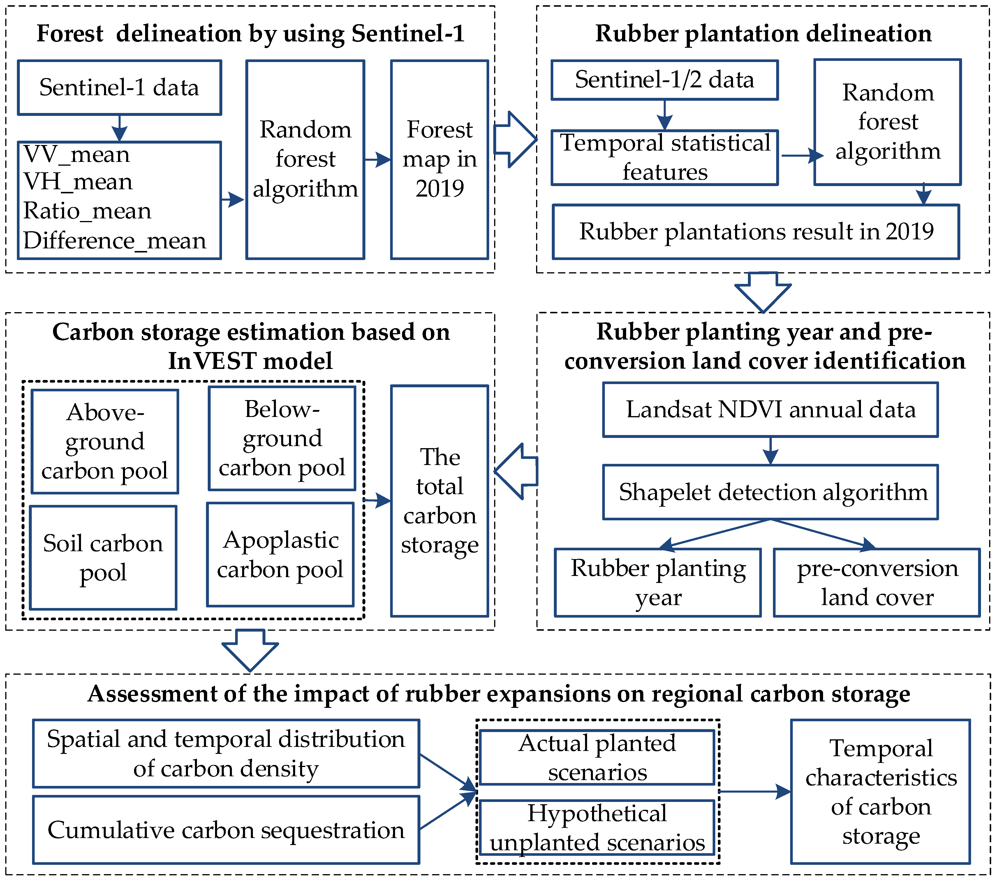
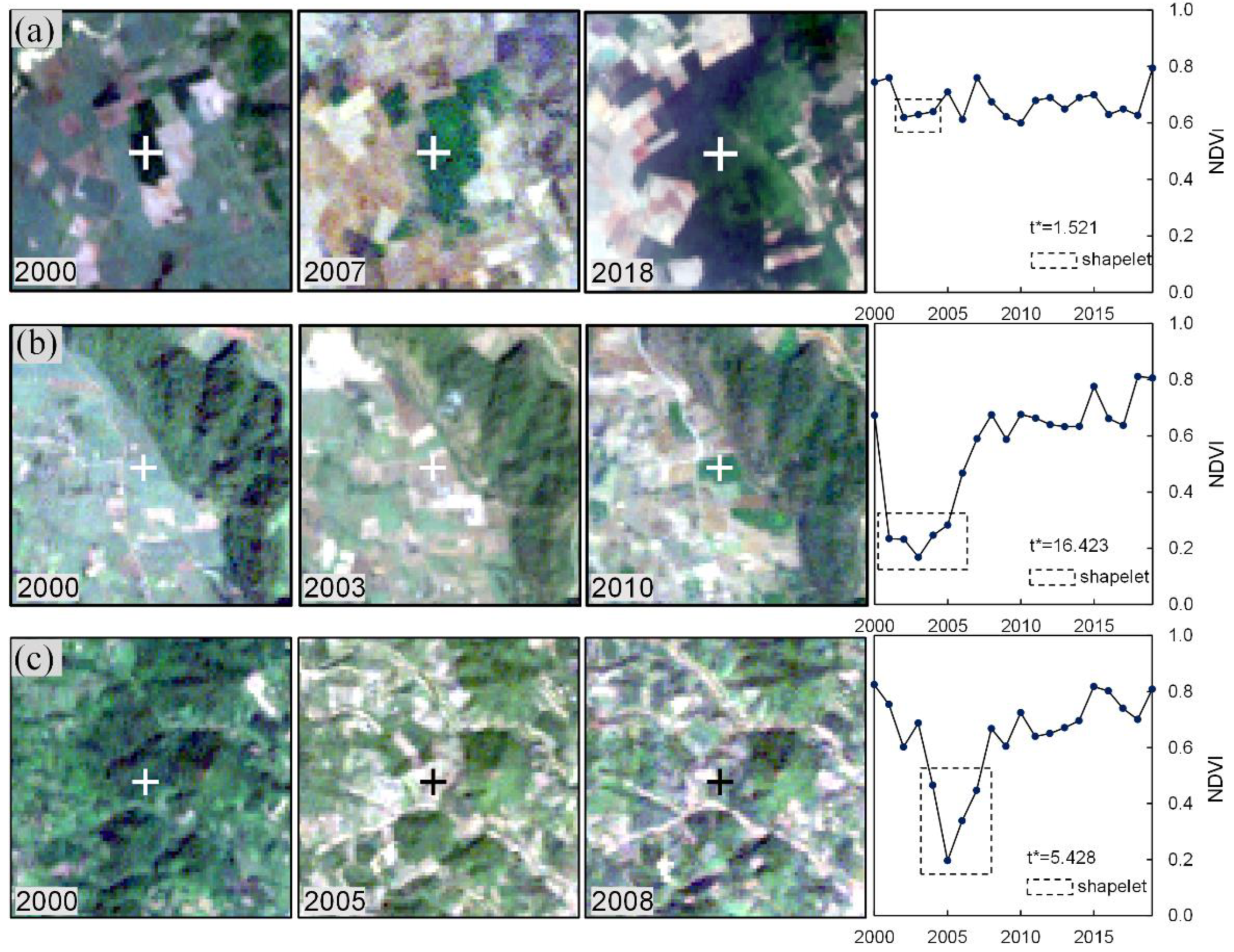
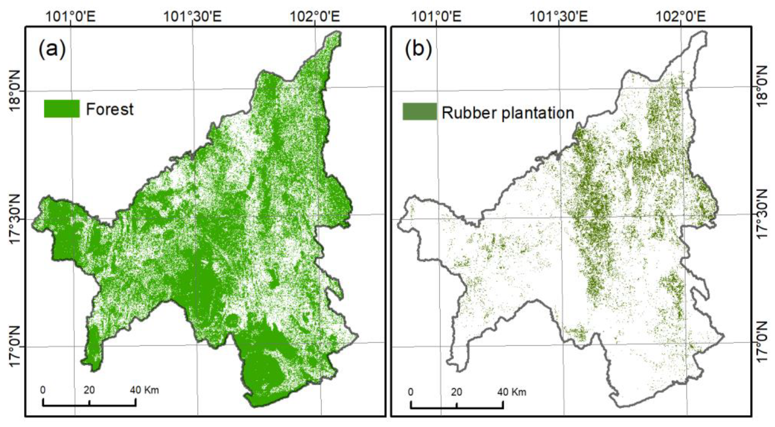
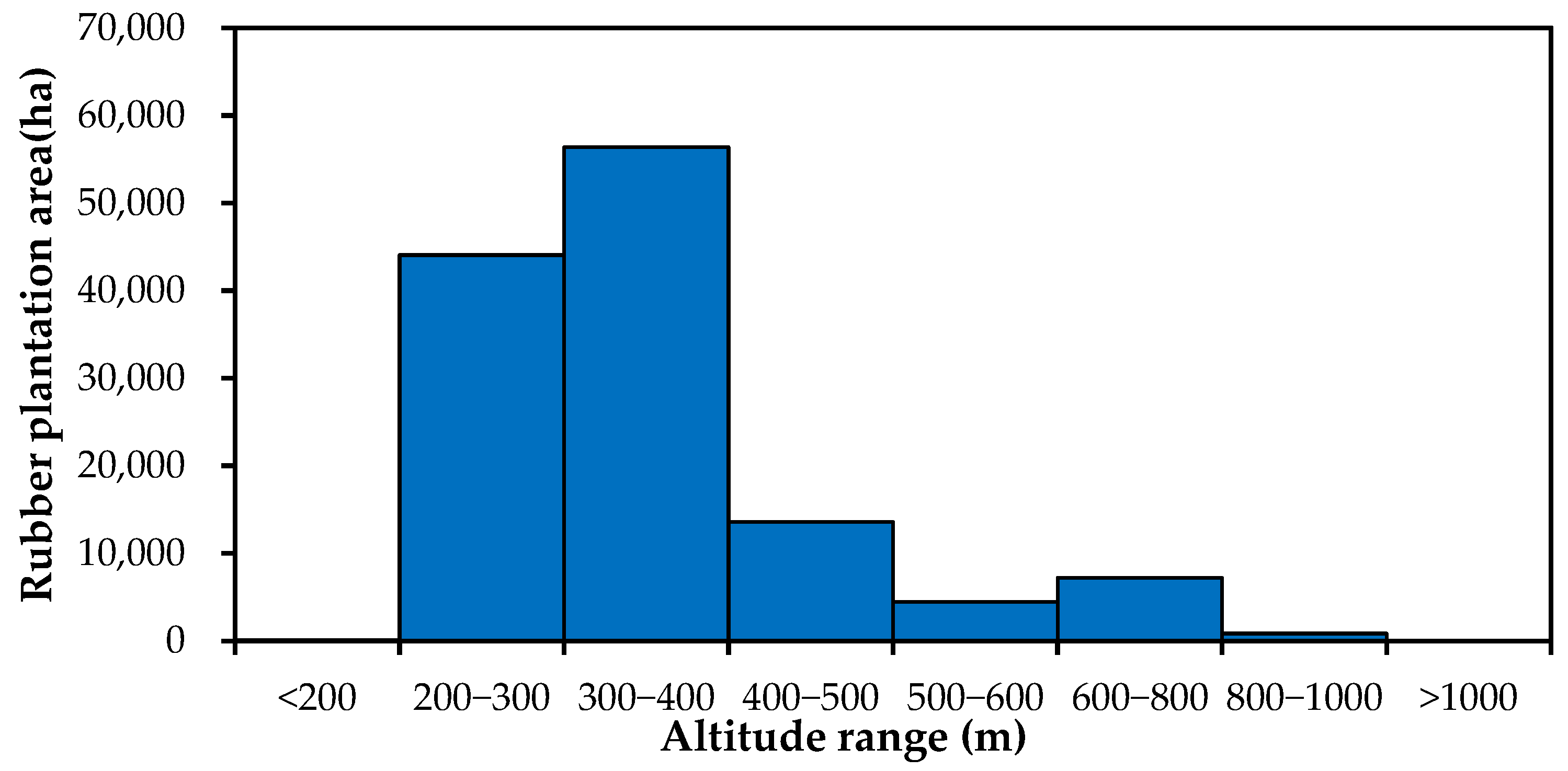
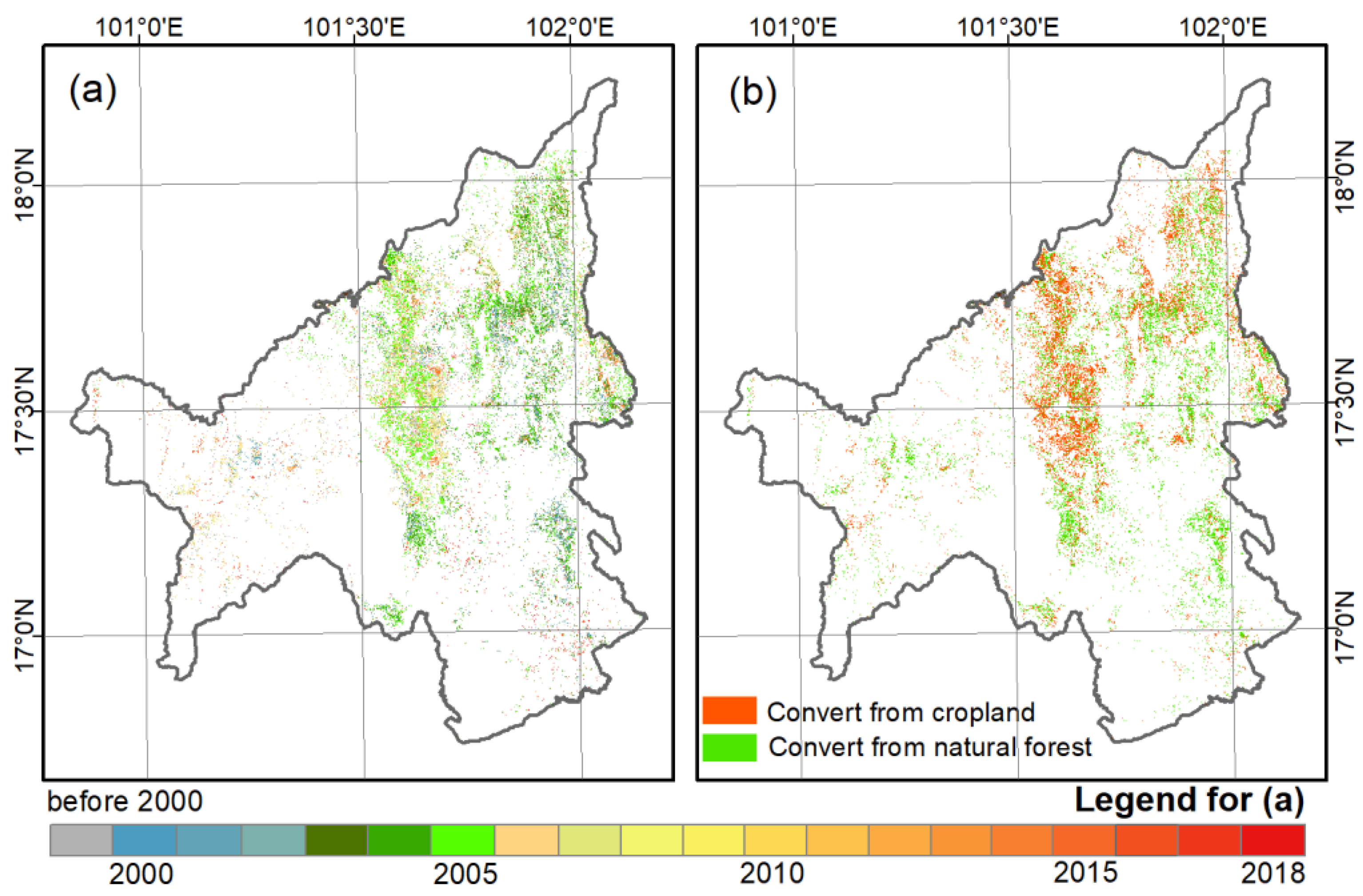
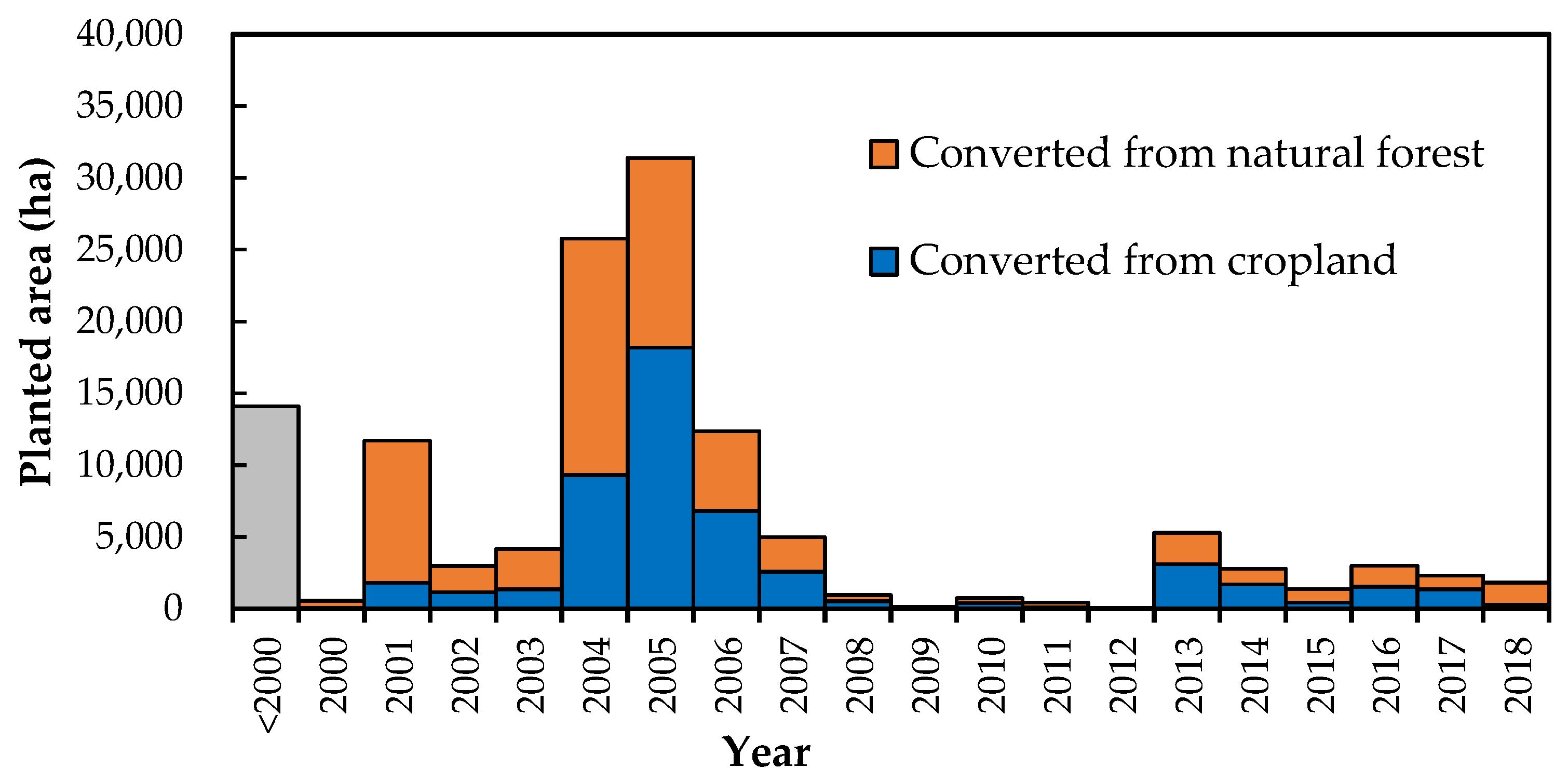
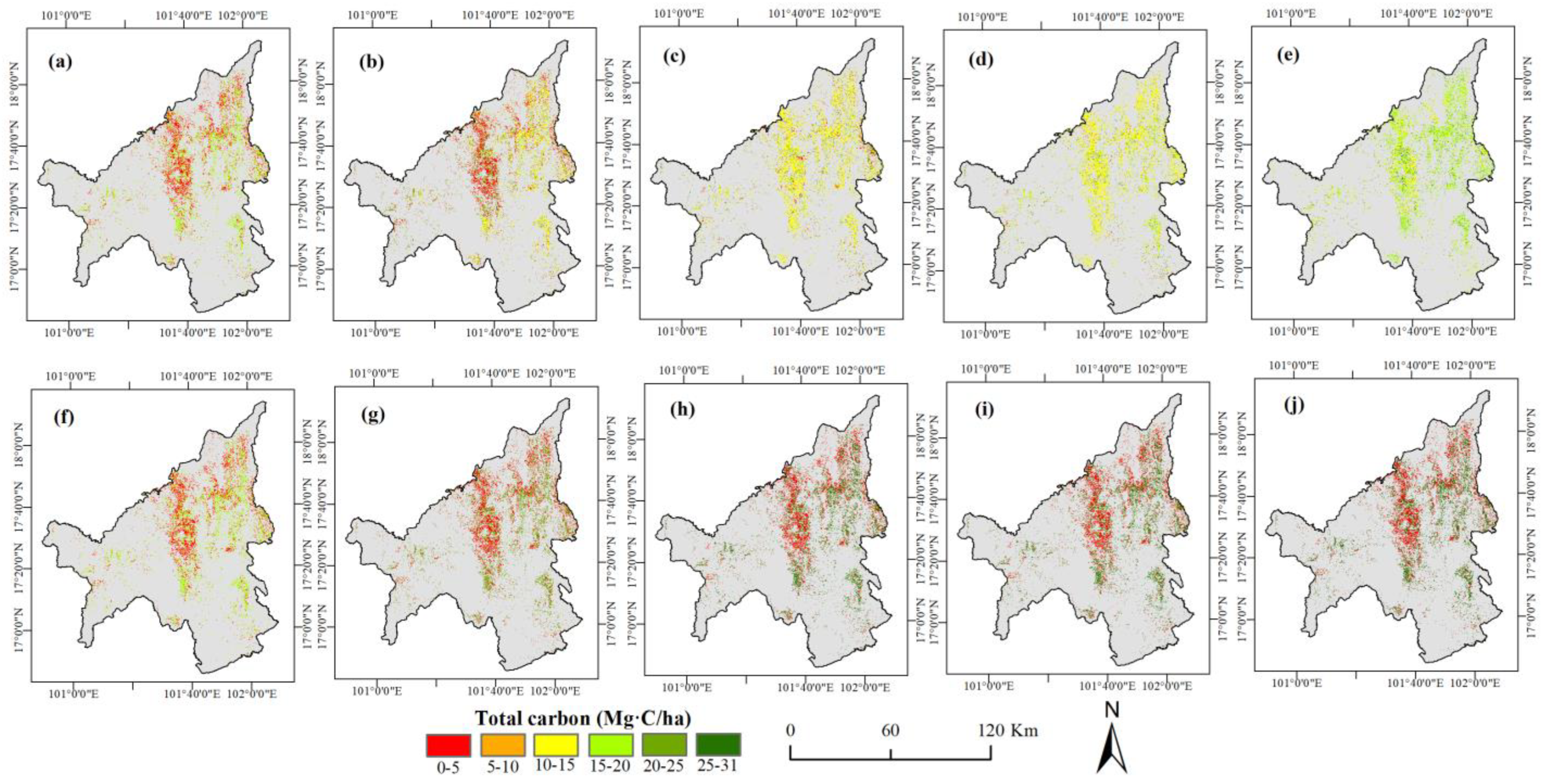
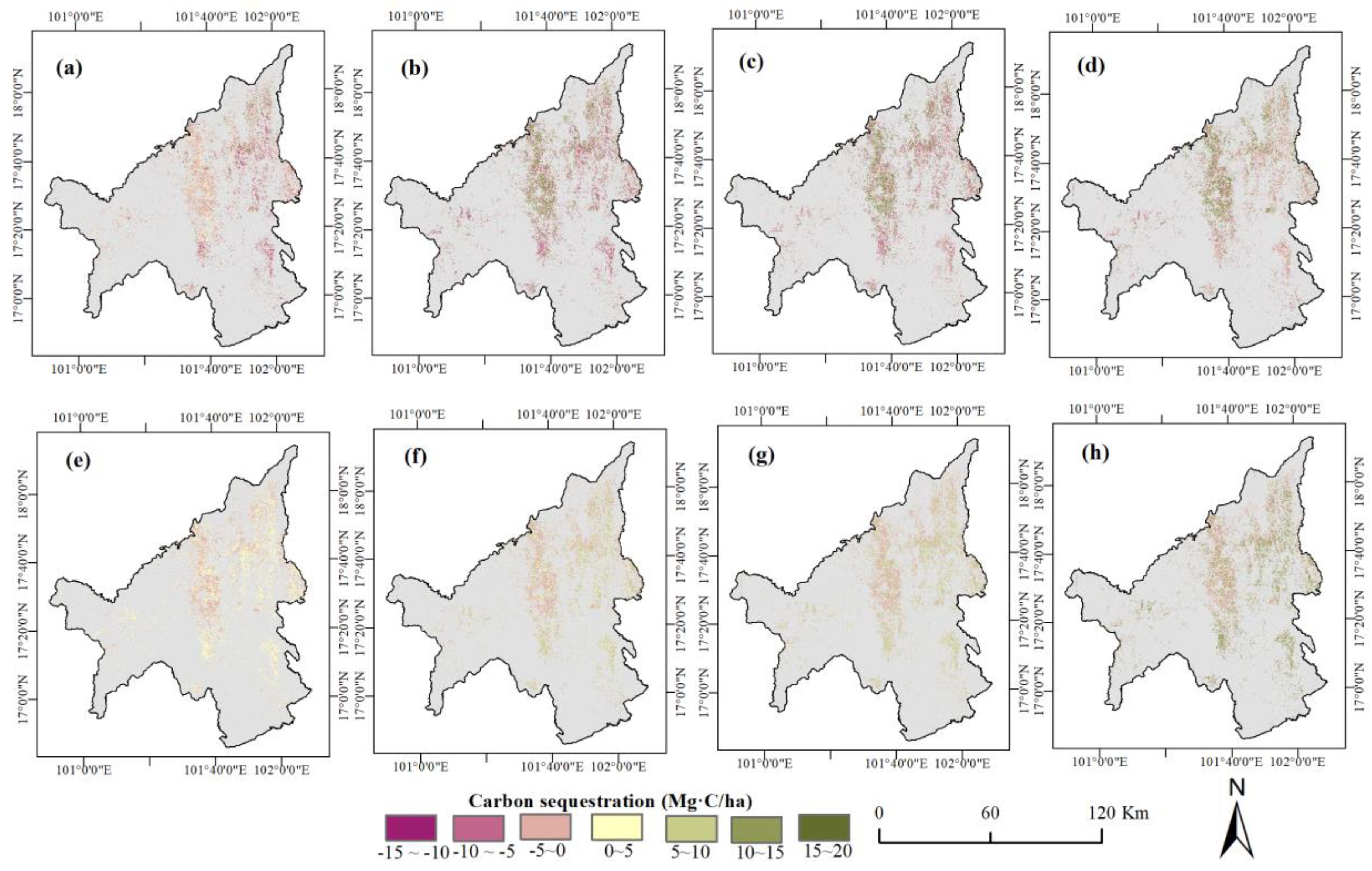
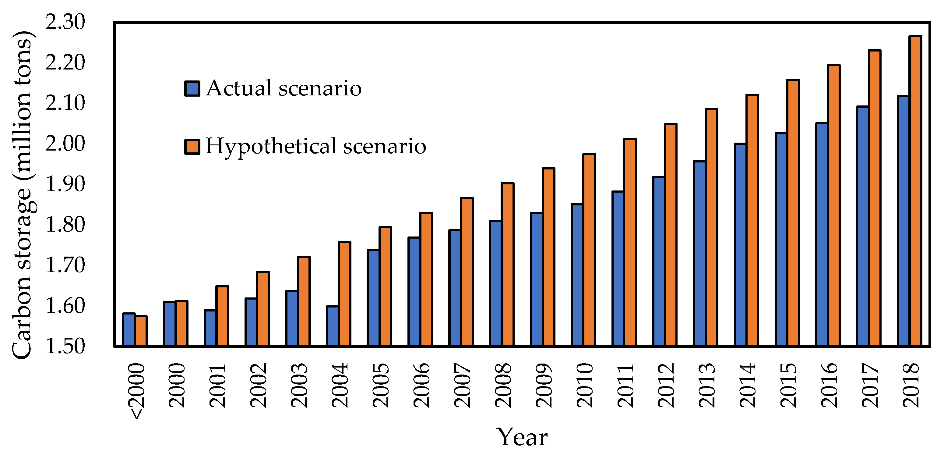
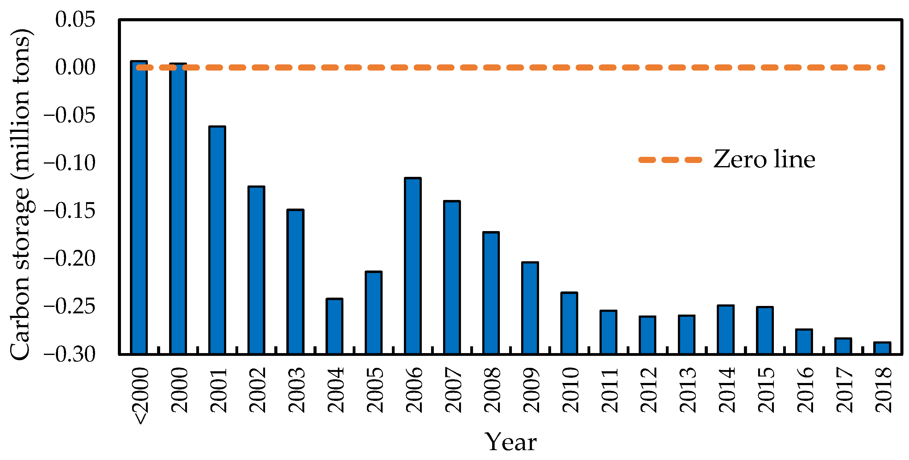
Table 1.
List of Landsat images used to build the time-series stack.
| Year | Date | Sensor | Year | Date | Sensor |
|---|---|---|---|---|---|
| 1999 2000 2001 2002 2003 2004 2005 2006 2007 2008 2009 | 1999/11/16 2000/11/10 2001/1/05 2002/11/08 2003/3/16 2004/11/5 2005/11/24 2006/11/27 2007/1/14 2008/3/5 2009/3/8 | ETM+ TM ETM+ ETM+ ETM+ TM TM TM TM TM TM | 2010 2011 2012 2013 2014 2015 2016 2017 2018 2019 | 2010/2/23 2011/1/25 2012/4/25 2013/11/30 2014/1/17 2015/1/4 2016/4/12 2017/2/10 2018/2/13 2019/4/21 | TM TM ETM+ OLI OLI OLI OLI OLI OLI OLI |
Publisher’s Note: MDPI stays neutral with regard to jurisdictional claims in published maps and institutional affiliations. |
© 2022 by the authors. Licensee MDPI, Basel, Switzerland. This article is an open access article distributed under the terms and conditions of the Creative Commons Attribution (CC BY) license (https://creativecommons.org/licenses/by/4.0/).
Share and Cite
MDPI and ACS Style
Huang, C.; Zhang, C.; Li, H. Assessment of the Impact of Rubber Plantation Expansion on Regional Carbon Storage Based on Time Series Remote Sensing and the InVEST Model. Remote Sens. 2022, 14, 6234. https://doi.org/10.3390/rs14246234
AMA Style
Huang C, Zhang C, Li H. Assessment of the Impact of Rubber Plantation Expansion on Regional Carbon Storage Based on Time Series Remote Sensing and the InVEST Model. Remote Sensing. 2022; 14(24):6234. https://doi.org/10.3390/rs14246234
Chicago/Turabian StyleHuang, Chong, Chenchen Zhang, and He Li. 2022. "Assessment of the Impact of Rubber Plantation Expansion on Regional Carbon Storage Based on Time Series Remote Sensing and the InVEST Model" Remote Sensing 14, no. 24: 6234. https://doi.org/10.3390/rs14246234
Note that from the first issue of 2016, this journal uses article numbers instead of page numbers. See further details here.