

Optimal Rain Gauge Network Design Aided by Multi-Source Satellite Precipitation Observation

1
College of Civil Engineering and Architecture, Zhejiang University, Hangzhou 310058, China
2
Zhejiang Institute of Hydraulics & Estuary (Zhejiang Institute of Marine Planning and Design), Hangzhou 310020, China
3
Jiangsu Provincial Planning and Design Group, Nanjing 210019, China
4
College of Computer and Information, Hohai University, Nanjing 210098, China
5
Key Laboratory for Geographical Process Analysis and Simulation of Hubei Province, Central China Normal University, Wuhan 430079, China
6
College of Urban and Environmental Sciences, Central China Normal University, Wuhan 430079, China
*
Author to whom correspondence should be addressed.
Remote Sens. 2022, 14(23), 6142; https://doi.org/10.3390/rs14236142
Submission received: 8 September 2022
/
Revised: 23 November 2022
/
Accepted: 30 November 2022
/
Published: 3 December 2022
(This article belongs to the Special Issue In Situ Data in the Interplay of Remote Sensing)
Abstract
:Optimized rain gauge networks minimize their input and maintenance costs. Satellite precipitation observations are particularly susceptible to the effects of terrain elevation, vegetation, and other topographical factors, resulting in large deviations between satellite and ground-based precipitation data. Satellite precipitation observations are more inaccurate where the deviations change more drastically, indicating that rain gauge stations should be utilized at these locations. This study utilized satellite precipitation observation data to facilitate rain gauge network optimization. The deviations between ground-based precipitation data and three types of satellite precipitation observation data were used for entropy estimation. The rain gauge network in the Oujiang River Basin of China was optimally designed according to the principle of maximum joint entropy. Two optimization schemes of culling and supplementing 40 existing sites and 35 virtual sites were explored. First, the optimization and ranking of the rain gauge station network showed good stability and consistency. In addition, the joint entropy of deviation was larger than that of ground-based precipitation data alone, leading to a higher degree of discrimination between rain gauge stations and enabling the use of deviation data instead of ground-based precipitation data to assist network optimization, with more reasonable and interpretable results.

1. Introduction
Rainfall data constitute the most important information source for hydrological forecasting, flood monitoring and simulation, and water resource development and utilization [1]. Rain gauge station networks are the most direct providers of precipitation data. The completeness and accuracy of the data acquired by such networks directly influences the development of various hydrological work. At present, although rain gauge station networks can cover most monitoring areas, two common issues remain in the construction of these networks: (1) there are gaps in the monitored region, and (2) redundant rain gauge stations exist in part of the region. A high rain gauge station density is always desirable in basins but is rarely found [2]; hence, there is no specific answer to the key question of what size of rain gauge station network is sufficient to record the spatial-temporal variability of the rainfall in a basin [3]. A properly designed rain gauge station network can minimize input and maintenance costs and ensure the overall accuracy of the precipitation monitoring data, improving the ability to capture short-term heavy and light rainfall, and accurately reflecting the spatial-temporal distribution of rainfall at different scales. The main goal of rain gauge station network design optimization is to ensure that the provided precipitation data can satisfy the application requirements of different spatial-temporal scales. It is thus necessary to determine the number of rain gauge stations and their optimal locations for installation, which generally includes eliminating redundant rain gauge stations [4,5], adding new stations [6,7,8], and rearranging the stations [9].
Researchers have proposed many quantitative methods for optimal rain gauge station network design. These mainly include statistical methods such as the Kriging [10,11], Copula [8,12], cross-correlation [13,14,15], model output error [16], multi-criteria decision-making [17,18], and information entropy [4,19,20,21,22] methods. Statistical methods optimize rain gauge station networks by reducing monitoring errors, whereas multi-criteria decision-making methods do so by determining an overall objective and multiple criteria. Most methods of these types consider only a single rain gauge at a time but not the rain gauge station network as a whole, neglecting the transferability, relevance, and attenuation of information, and are limited in their network optimization abilities [23]. In information entropy methods, the amount of information that can be accommodated between the rain gauge stations is increased, and the information redundancy is reduced through the comparison and selection of multiple rain gauge stations. In recent years, various combined methods based on information entropy have been widely used in rain gauge station network optimization [8,22,24].
The easiest way to apply information entropy to rain gauge station network optimization is to sort the importance of the rain gauge stations according to their information entropy. However, this approach ignores the relevance of information between rain gauge stations. Consequently, many indicators of entropy that consider the information relevance among rain gauge stations have been applied, including maximizing the joint information entropy [4,25], minimizing the transfer information [24], and minimizing the total correlation [26] among rain gauge stations, and many derived indicators, such as the trans-information-distance relation [7,13,27] and value of monitoring index [8]. The benefits of the principle of maximum entropy include the robustness of the description of the posterior probability distribution because it aims to define a less biased outcome. This is because neither the models nor the measurements are completely certain [20]. With the rain gauge stations already known, although it is always possible to determine the ranking results of these gauge stations based on their quantitative importance, there remains room for improvement in rain gauge station network optimization based on information entropy theory. First, many studies have shown that topography has an important effect on the heterogeneity of the spatial-temporal distribution of rainfall [8,9]. For example, Tiwari et al. [3] found that rain gauge stations at high altitudes are extremely important, independent of the rain gauge station network size and data acquisition frequency. Although information entropy based on precipitation data can reflect the same trend to a certain extent, quantification is difficult, leading to poor interpretability. Second, the redundancy of the information entropy among rain gauge stations in the region is large, such that the rain gauge stations of different importance rankings are not very distinguishable regardless of the ranking being based on joint information entropy, transfer information, or total correlation.
Satellite precipitation observation has become the most important source of precipitation data besides ground-based precipitation monitoring. Although the data accuracy is less than that of ground-based precipitation monitoring data, satellite precipitation observation data have wide coverage and a fast update frequency. Further, they are capable of providing the “face” precipitation data of the region of interest, unlike ground-based “point” precipitation data. Using ground-based precipitation monitoring data for reference, researchers have adopted the Nash-Sutcliffe model efficiency coefficient, root-mean-squared error, and relative deviation to evaluate the accuracy of mainstream satellite precipitation data, such as GPM IMERGE, GSMaP, and PERSIANN and their suitability for hydrological applications [28,29], and to discuss the capability of satellite precipitation observations to capture heavy and light rainfall [30]. In addition, researchers have conducted extensive investigations on bias correction and fusion of satellite precipitation data, launching numerous precipitation data reanalysis products, and enriching the application scenarios of satellite precipitation data [31,32].
It is commonly known that surface characteristics including topography, such as elevation, slope, and aspect, and vegetation, such as NDVI, have important effects on the error of satellite precipitation estimation. Most studies on bias correction and data fusion of satellite precipitation data have adopted these parameters as correction factors [33,34,35]. The deviation between satellite precipitation observation and ground-based precipitation data is the most intuitive measure of the uncertainty of satellite precipitation observations. By estimating the information entropy of the deviation between satellite precipitation observation and ground-based precipitation data, the degree of disorder in the random errors between the two can be characterized more effectively. The higher this information entropy, the more random the errors, indicating that the ability of the satellite to capture ground rainfall is poorer. From the perspective of satellite precipitation observation, it is necessary to focus on retaining or adding rain gauge stations where data are inaccurately captured by the satellite precipitation observation, especially with the objective of achieving better data fusion.
Some researchers have already started to use ground-based radar to facilitate optimal rain gauge station network design [36,37]. These scholars have focused mainly on using radar-estimated precipitation to fill in the blank areas in rain gauge station networks, whereas studies on using satellite precipitation observation data to facilitate the optimization of large-scale ground-based rain gauge station networks remain relatively rare [38]. In this paper, three types of satellite precipitation observation data (GPM IMERGE, GSMaP, and PERSIANN) were used, and the information entropy of the deviation in the precipitation data was estimated to maximize the joint information entropy. On this basis, a method of using satellite precipitation observations to facilitate the optimal ground-based rain gauge station network design was proposed, and an empirical study was performed in the Oujiang River Basin in China.
2. Method
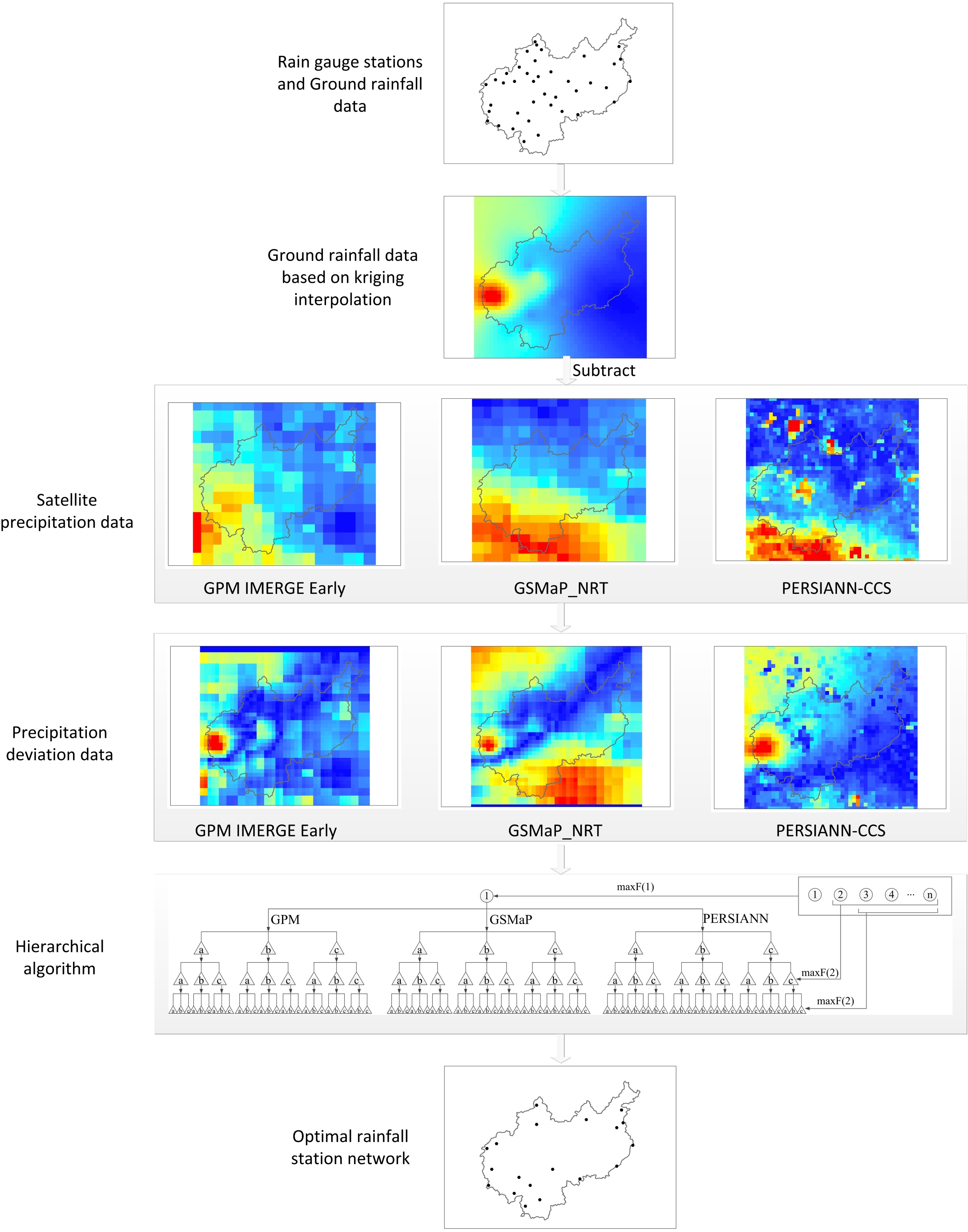
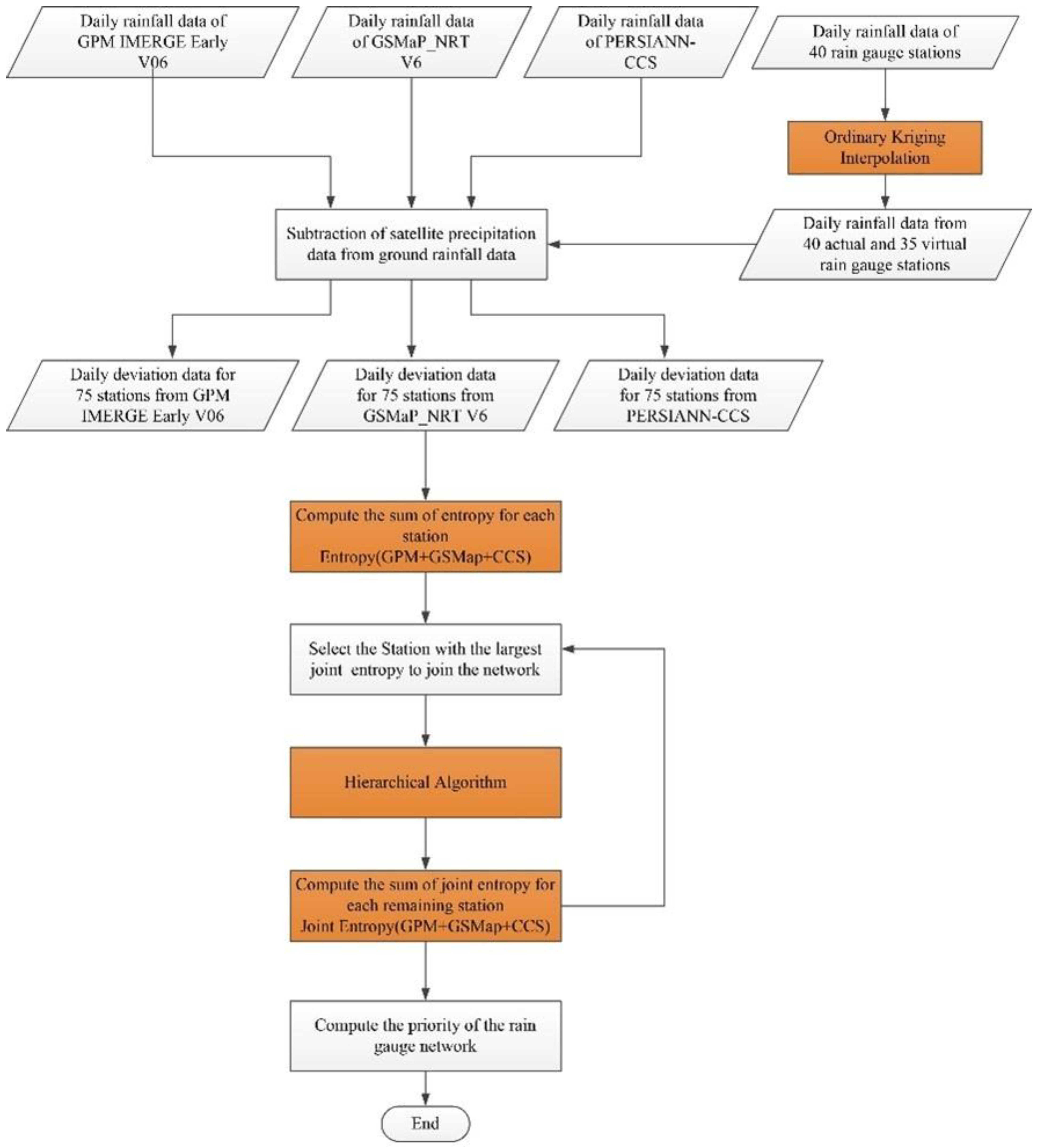
The process of rain gauge station network design optimization assisted by satellite precipitation data is illustrated in Figure 1, and mainly includes the following steps: (1) Daily precipitation data were collected from 40 rain gauge stations in the study region, and the three sets of uncorrected real-time satellite-based daily rainfall observation data (i.e., GPM IMERGE Early V06, GSMap_NRT V6, and PERSIANN−CCS) were acquired. (2) Kriging interpolation was adopted to obtain the daily precipitation data at 35 virtual (non-existent) rain gauge stations based on the daily precipitation data from the 40 actual rain gauge stations. (3) The daily precipitation data from all 75 rain gauge stations (40 actual and 35 virtual rain gauge stations) were subtracted by the three sets of satellite-based precipitation data to obtain three sets of daily rainfall deviation data at each of the 75 rain gauge stations. (4) A hierarchical algorithm based on joint information entropy was designed to decompose the daily rainfall deviation data at the stations layer by layer, while calculating the joint information entropy simultaneously, so as to add the station with the maximum joint information entropy into the optimization ranking for the station network. (5) An order of priority for all rain gauge stations was thus obtained. Section 2.1, Section 2.2 and Section 2.3 describe kriging interpolation, information entropy, and the hierarchical algorithm in detail, respectively.
2.1. Kriging Interpolation Technique
The Kriging interpolation is a regression algorithm for spatial modeling and prediction of random processes or random fields based on covariance functions. As it can lead to the best linear unbiased prediction (BLUP), it is also called spatial BLUP in geostatistics. The original Kriging algorithm is called ordinary Kriging (OK), and the commonly used improved algorithms include the universal Kriging (UK), co-Kriging (CK), and disjunctive Kriging (DK) algorithms. The OK algorithm has been used by many researchers to interpolate rainfall at virtual (candidate) rain gauge stations [9,10,24]. The OK interpolation equation is as follows:
where ) is the estimated rainfall Z at location , is the observed rainfall at location , N is the number of observation sites for the interpolation, and is the weight of the observed rainfall at location .
In Kriging interpolation theory, both the unbiased and optimal conditions must be met, as shown in the following equations:
where Equation (3) can be solved by utilizing Lagrange multipliers, based on the following equations:
Here, represents the Kriging variance, the error related to the Kriging estimator; is the Lagrange multiplier; and is the value of the variogram between the i-th rain gauge station and reference station .
2.2. Information Entropy
Shannon [39] proposed the theory of information entropy based on probability, where the information entropy is a measure of the uncertainty of random variables. In a network of hydrological stations, information entropy can be used to quantify the information contained in the hydrological data series (precipitation, flow, etc.) measured at the station. In this paper, the information entropy of the rainfall deviation between the rain gauge stations and satellite was estimated. Assuming that the precipitation measured by the rain gauge stations on a certain day is pground and the satellite precipitation observation is psatellite, the daily precipitation deviation can be represented as the absolute difference between the ground-based precipitation data and satellite precipitation observation:
Assuming that the daily precipitation deviation series is represented by the random variable , whose probability density function is , the information entropy of the random variable can be represented by:
where n represents the different values taken by the samples. When applied to the multivariate case, the joint information entropy for the random variables ,,…, in the d-dimensional space can be defined as
where is the joint probability density function of the random variables of the d-dimensional space and , , …, are the different values taken by the random variables , , …, of the space. When applied to a rain gauge station network, and represent respectively the total amount of information of the daily rainfall deviation from a single rain gauge station and multiple stations.
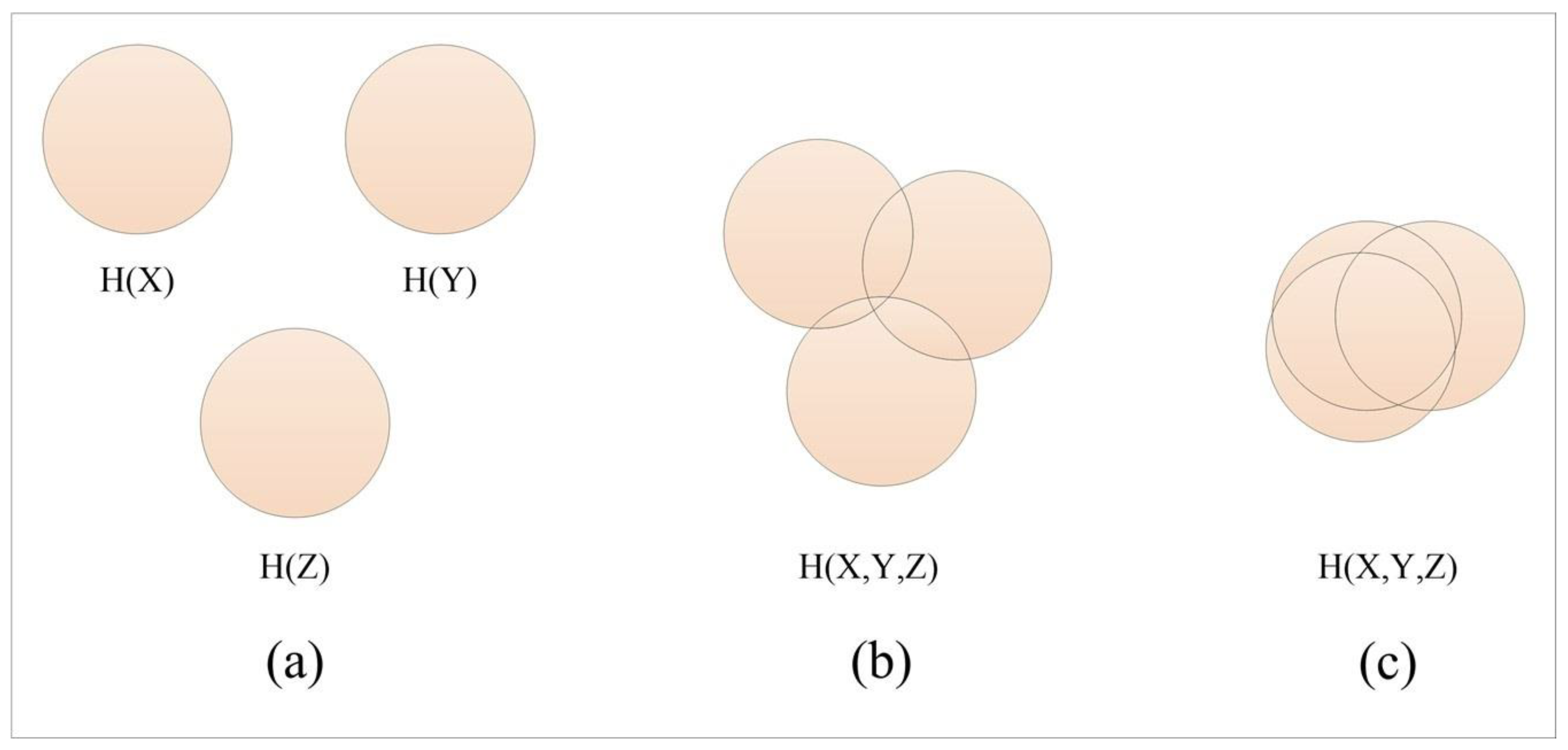
Figure 2 provides a schematic diagram of the information entropy and joint information entropy of the rain gauge stations. In Figure 2a, the size of the information entropy is represented by the area of the circle indicating the rainfall deviation of the station. In Figure 2b,c, the area of all the circles projected onto the plane (where the overlapping area is counted only once) represents the joint information entropy between the stations. The rain gauge station network optimization process that aims to maximize the joint information entropy attempts to obtain the most information using the fewest rain gauge stations. As shown in Figure 2b, when the degree of overlapping between the rain gauge stations X, Y, and Z is low, it is necessary to retain more rain gauge stations to avoid information loss. In contrast, Figure 2c shows that when the degree of redundancy of the information entropy between the stations is high, it is necessary to remove some of the rain gauge stations.
Equations (8) and (9) are both for discrete random variables. In reality, rainfall deviations are not discrete, but rather continuous and can take any decimal value. Strictly speaking, the above Equations (8) and (9) should be represented by integrals [9]; hence, it is necessary to discretize the rainfall deviation data. Keum et al. [40] and Li et al. [8] proposed a floor function rounding (FFR) to discretize the precipitation data:
where represents the original observation data, indicates the discretized data, G is the floor function that rounds down the independent variable to the nearest integer, and is a parameter of the function. FFR is an interval-based rounding method, which treats all data in a certain numerical interval as having the same value. For example, when , the discretized intervals are [0, 0.5], [0.5, 1.5], and [1.5, 2.5]. In this paper, . To ensure that observation data with the same integer part are in the same interval, the FFR equation was modified to:
2.3. Hierarchical Algorithm
Joint information entropy, transfer information, and total correlation are concepts involving two or more stations. As such, it is extremely important to clarify which station is used as the first station. In many studies, the rain gauge station with the maximum information entropy is used as the first station. Among the remaining stations, the most important station is then determined based on a certain objective optimization rule (e.g., maximum information entropy, minimum transfer information, or minimum total correlation) [9,41,42,43].
For n rain gauge stations, three sets of rainfall deviation data (GPM, GSMaP, and PERSIANN) are available. In this paper, the information entropies of these three sets of data are given the same weight, and the rain gauge station network optimization rule is as follows:
where represent respectively the information entropies of the GPM IMERGE, GSMaP, and PERSIANN rainfall deviation data at station X; are respectively the joint information entropies calculated using the GPM IMERGE, GSMaP, and PERSIANN satellite precipitation deviation data at d rain gauge stations. The optimization steps for the rain gauge station network are as follows:
Step 1: For each of the n stations, the average information entropy is calculated, and the station with , i.e., station i with the maximum information entropy, is used as the first station.
Step 2: For each of the remaining n − 1 stations, the average joint information entropy between that station and station i is calculated, and the station with , i.e., station j with the maximum joint information entropy, is selected as the second station.
Step 3: For each of the remaining n − 2 stations, the average joint information entropy between that station and stations i and j is calculated, and the station with , i.e., station k with the maximum joint information entropy is selected as the third station.
Step n − 1: For both of the remaining two stations, the average joint information entropy between that station and the previous n − 2 stations is calculated, and the station with , i.e., station m with the maximum joint information entropy, is selected as the (n − 1)-th station.
Step n: For the final station, the average joint information entropy with respect to the previous n − 1 stations is the total joint information entropy of the rain gauge station network. As such, the importance ranking of the n stations is completed.
In the previous steps, each calculation of the joint information entropy between stations is an independent process, and it is necessary to calculate the various joint information entropies for (n − 1) + (n − 2) + (n − 3) + …… + 1 = times. To simplify the algorithm and improve the calculation efficiency, researchers have proposed a hierarchical algorithm based on joint information entropy [44]. This algorithm classifies the observation data of candidate sites, divides the combinations of observation data between sites layer by layer, and thus calculates of joint information entropy between sites. It has been applied to bridge diagnosis [45], wind prediction [46], and sensor placement optimization in water supply network [47].
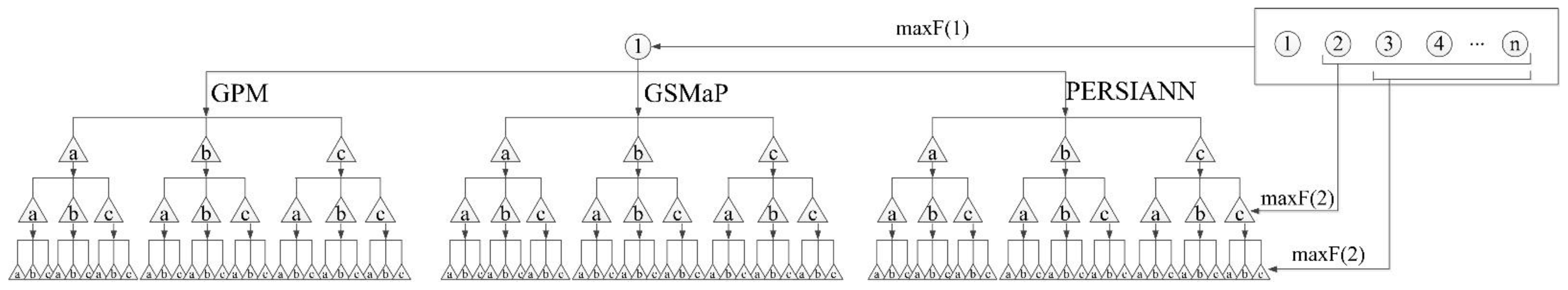
Figure 3 provides a schematic diagram of joint information entropy calculated using the layer-by-layer algorithm based on satellite precipitation deviations. Although the steps of this algorithm are exactly the same as those of the previous algorithm, the calculation of the joint information entropy between stations is simplified. For illustrative purposes, it is assumed that the precipitation deviations at each station consist of only a, b, and c.
First, the station with the maximum information entropy for the three sets of satellite precipitation deviation data is determined and selected as the first station. The dates on which the three sets of satellite-observed daily precipitation deviations a, b, and c appear can be summarized into the following sets: GPMa = {ta1, ta2, ta3, …, tai}, GPMb = {tb1, tb2, tb3, …, tbj}, GPMc = {tc1, tc2, tc3, …, tck}, GSMaPa = {ta1, ta2, ta3, …, tau}, GSMaPb = {tb1, tb2, tb3, …, tbv}, and GSMaPc = {tc1, tc2, tc3, …, tcw}. It is known that i + j + k = u + v + w.
Subsequently, the joint information entropy of the first station with the other stations is calculated to determine the distribution of the precipitation deviations of the other stations on the dates on which the three sets of satellite-observed daily precipitation deviations at the first station are, respectively, a, b, and c, i.e., to obtain the set of dates on which (a, a), (a, b), (a, c), (b, a), …, (c, c) appear between two stations. The probabilities of the occurrence of (a, a), (a, b), (a, c), (b, a), …, (c, c) precipitation deviation combinations in the three sets of satellite observation data are calculated individually to determine the joint information entropy between any two stations. Once the station with the maximum average joint information entropy is determined and used as the second station, the date sets of (a, a), (a, b), (a, c), (b, a), …, (c, c) appearing with the three sets of satellite observation data can be determined.
The same process can be implemented to select the third optimal station, i.e., to determine the date sets of (a, a, a), (a, a, b), …, (c, c, c) for the three sets of satellite-based data, and thus the station with the maximum average joint information entropy for the three-station combinations. This decomposition is implemented layer by layer until the division of all observation data is completed, and the optimal sequence of rain gauge stations is obtained.
3. Study Area and Dataset
3.1. Study Area
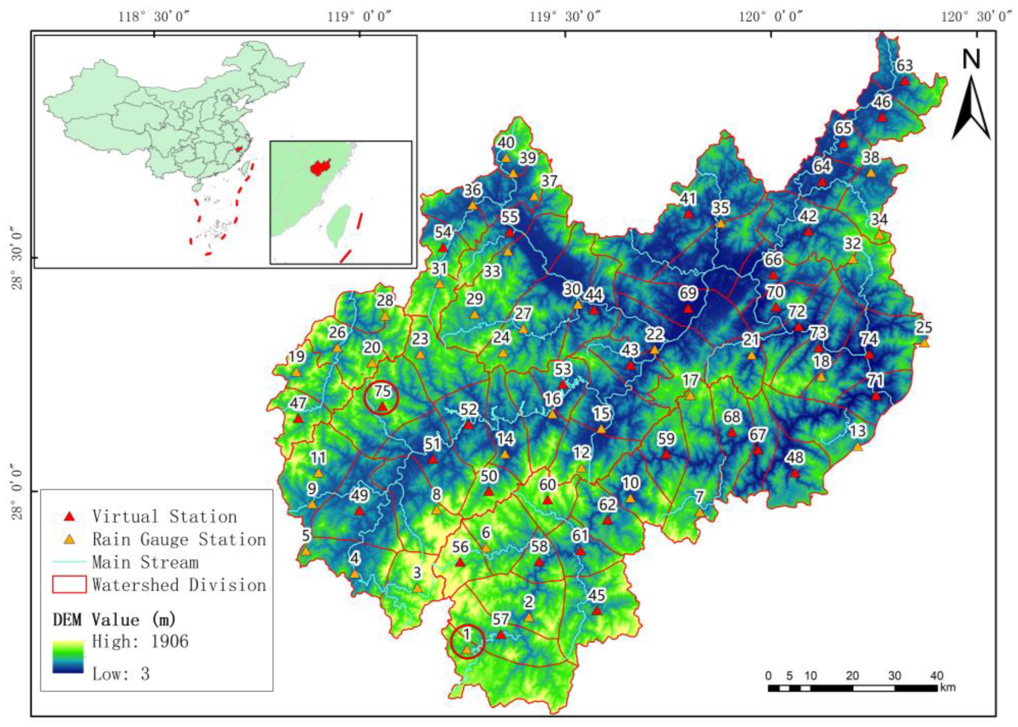
In this research, the Oujiang River Basin located in Zhejiang Province, China, was selected as the study area. Figure 4 shows the scope of the Oujiang River Basin and the distribution of the water system from the main stream. Oujiang River is the second largest river passing through Zhejiang Province and flows from the west to the east, running through the mountainous area in southern Zhejiang Province and passing by cities such as Lishui and Wenzhou. The Oujiang River Basin covers an area of 13,103 km2, with an elevation difference near 2000 m. The main stream is 388 km long and can be divided into three sections from the source to the estuary (Longquanxi River, Daixi River, and Oujiang River), eventually entering the East China Sea at the Wenzhou Bay in Wenzhou. The Oujiang River has an average annual runoff of 20.27 × 10⁹ m3, with a hydropower reserve of 1.9 × 10⁶ kW. The Oujiang Estuary is the fifth main estuary in China after the Yangtze River Estuary, Yellow River Estuary, Pearl River Estuary, and Qiantang River Estuary, with a well-developed shipping industry.
In this investigation, the optimal design of existing and newly added rain gauge stations was studied. For the optimal design of newly added rain gauge stations, it was necessary to select the optimal stations from virtual rain gauge stations [8,21,48,49,50]. Previous scholars have usually set virtual stations at the centers of generated regular grids and then determined the locations of the new stations to be added based on the specific optimization objectives [48,49]. Li et al. [8] created Thiessen polygons based on the existing rain gauge stations and used the vertices of the Thiessen polygons as the locations of the virtual stations. To relocate the existing stations, Yeh et al. [9] adopted the idea of regular grids and selected the grid centers as the locations of the candidate stations to be relocated. In the end, 6 optimal stations were selected from the 17 candidate rain gauge stations. As shown in Figure 4, we firstly divided the Oujiang River Basin into 16 sub-regions based on the concept of hydrological modelling and then further divided the 16 sub-regions into 64 computing units. Each computing unit was required to have one rain gauge station. If there was no rain gauge station in the computing unit, then a virtual rain gauge station was set in the geometric center of the computing unit. Figure 4 shows the 75 rain gauge stations in the study area, where the 40 existing rain gauge stations are marked with orange triangles and numbered from 1 to 40, and the 35 virtual rain gauge stations are marked with red triangles and numbered from 41 to 75.
3.2. Dataset
3.2.1. Daily Precipitation Data from Existing and Virtual Rain Gauge Stations
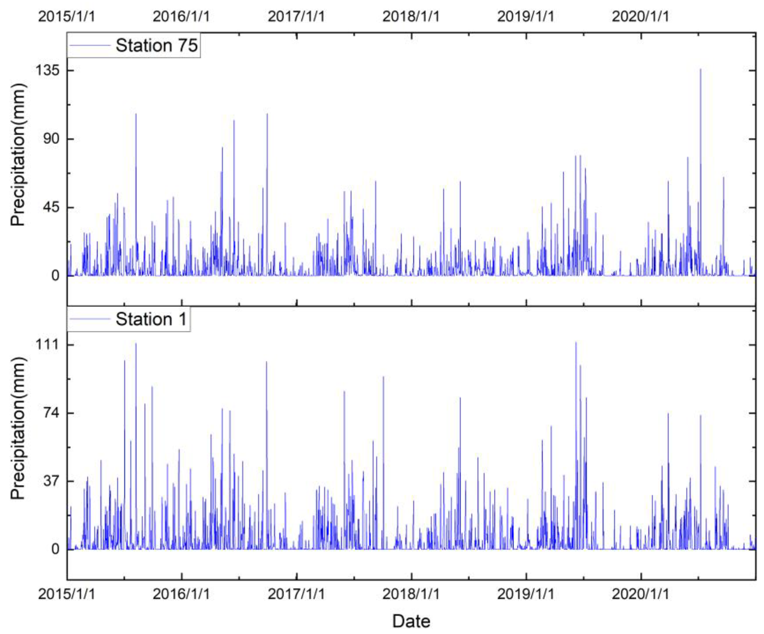
In this study, the daily precipitation data series acquired at the rain gauge stations from 1 January 2015 to 31 December 2020 (a total of 72 months) were selected. Each station provided 2192 daily data, where the daily precipitation data from virtual stations 41–75 were obtained using Kriging interpolation. Figure 5 shows the daily precipitation data series for stations 1 and 75, respectively. It can be seen from the figures that precipitation mainly occurs between May and September each year.
3.2.2. Satellite-Observed Daily Precipitation Data
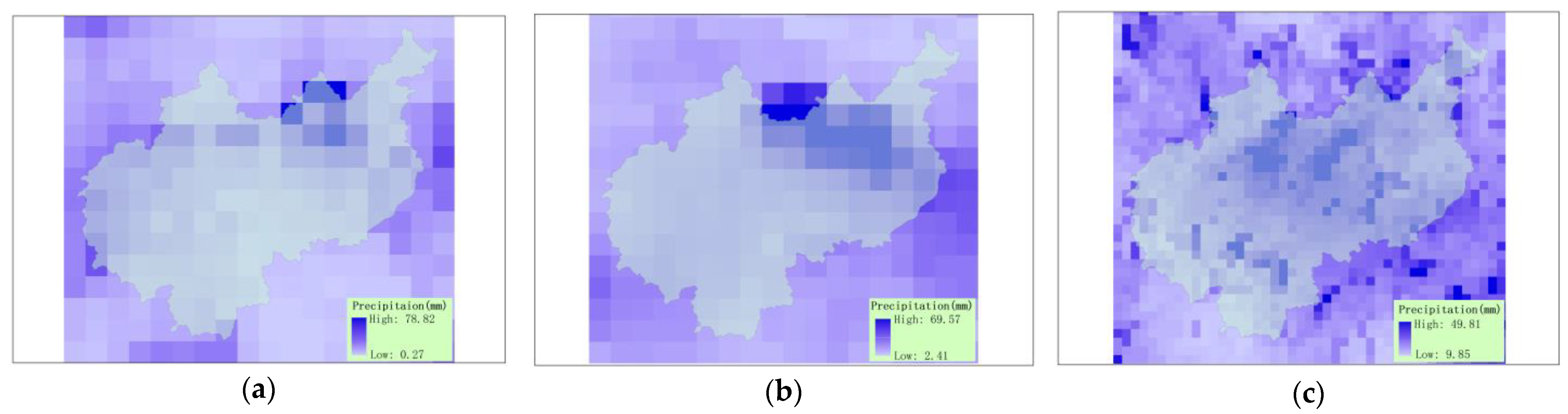
The uncorrected real-time GPM IMERGE Early V06, GSMaP_NRT V6, and PERSIANN−CCS precipitation data were selected from the GPM IMERGE, GSMaP, and PERSIANN satellite precipitation data products to facilitate ground-based rain gauge station network optimization. In addition to the real-time version, there are also near-real-time versions of satellite precipitation data, such as GPM IMERGE Final, GSMaP_Gauge, PERSIANN_CDR. These near-real-time versions are generally corrected with ground rain gauge stations. Researchers have conducted extensive research on the spatiotemporal accuracy of real-time data and near-real-time data [51,52,53], and the consensus is that near-real-time products have higher accuracy [54]. In order to avoid being affected by ground rainfall, our study did not use near-real-time products, but real-time products, which can amplify the deviation between satellite precipitation and ground rainfall and facilitate station network optimization. Figure 6 shows the spatial distribution of the three sets of satellite-based daily precipitation data in the Oujiang River Basin on 16 July 2020. The PERSIANN−CCS precipitation data have the highest spatial resolution of 0.04° × 0.04°, whereas the GPM IMERGE Early and GSMaP_NRT precipitation data have a spatial resolution of 0.1° × 0.1°. In order to facilitate comparative analysis, the GPM IMERGE Early and GSMaP_NRT data were interpolated so that the spatial resolution was consistent with PERSIANN−CCS (0.04° × 0.04°).
3.2.3. Daily Precipitation Deviation Data Set
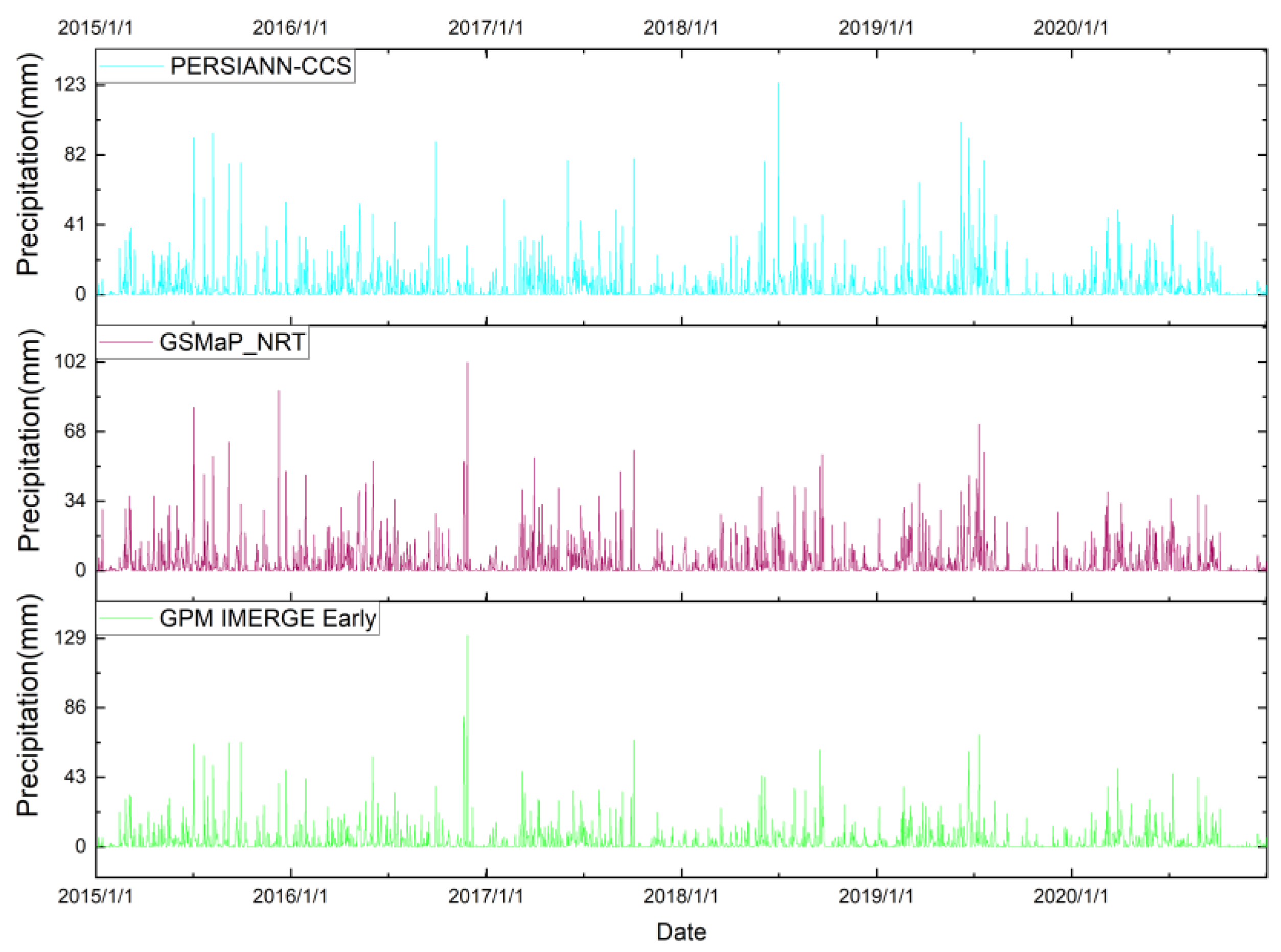
The locations of the 75 rain gauge stations in the three sets of gridded satellite precipitation data were determined, and the three sets of satellite-based daily precipitation data for each station were obtained. These data were then subtracted from the ground-based daily precipitation data, and the absolute values were used as the daily precipitation deviations at the 75 rain gauge stations. Figure 7 shows the daily precipitation deviations between the ground-based precipitation data observed at rain gauge station 1 and the GPM IMERGE Early, GSMaP_NRT, and PERSIANN−CCS data from 2015 to 2020.
4. Experiments and Results
4.1. Existing Rain Gauge Station Network Optimization
The station network design was optimized for the existing 40 rain gauge stations using five types of data: (1) GPM IMERGE Early daily precipitation deviation data; (2) GSMaP-NRT daily precipitation deviation data; (3) PERSIANN−CCS daily precipitation deviation data; (4) the combination of the above three sets of daily precipitation deviation data; and (5) ground-based precipitation data only. For data types (1)–(3) and (5), Equation (12) was simplified to Equation (13):
Table 1 shows the optimized ranking results of the station network with the 40 existing rain gauge stations achieved by using the above five types of data. The higher the ranking, the more important the station. In the rain gauge station selection process, a cumulative percentage threshold of the joint information entropy of rain gauge station with respect to that of all rain gauge stations was generally set, and redundant stations with smaller percentages were identified and eliminated. For example, Yeh et al. [9] selected 95% as the threshold for determining whether to retain a rain gauge station or not. Among the 17 rain gauge stations, the top 6 rain gauge stations provided 95% of the total joint information entropy, indicating that the other 11 rain gauge stations could be eliminated. In this paper, 98% of the total joint information entropy was used as the threshold for the selection of rain gauge stations to retain in the network. The joint information entropy of the stations whose numbers appear in bold in Table 1, when combined, can provide 98% of the total joint information entropy of all 40 stations that need to be retained. Although there is no reference standard for threshold setting, we can weigh it by the total increase in the joint information entropy. When the number of stations reaches a certain amount, the newly added station can only increase the joint information entropy by 0.01 or even 0.001, and there is no need to continue to increase the station.
The three sets of satellite precipitation deviation data were used individually to obtain the optimized ranking results of the rain gauge stations in the network, which showed a high degree of consistency, as there were 11 stations in common, accounting for 64%, 57%, and 61% of the numbers of stations to be retained in the three different rankings. In addition, the optimization schemes obtained using the combined satellite precipitation data and ground-based precipitation data both selected 19 stations to be retained, among which 15 were in common, accounting for 78% of the stations to be retained.
4.2. Rain Gauge Station Network Optimization Considering Virtual Stations
To optimize the rain gauge stations to be added, Wu et al. [55] optimized the existing rain gauge stations first, eliminated the redundant stations, and conducted an integrated analysis of the remaining stations with the rain gauge stations to be added, where the existing stations that were to be retained could no longer be eliminated in the subsequent analysis. Li et al. [8] decided to retain all existing stations and analyzed only which of the virtual stations should be added to the rain gauge station network. Yeh et al. [9] divided the study area into regular grids and set up a virtual station at each grid. By optimizing the virtual stations only and replacing the existing stations completely with the optimized virtual stations, the rearrangement of the rain gauge station network was achieved. Considering the fact that the addition of virtual stations inevitably influences the optimized ranking of the existing stations, the 40 existing and 35 virtual stations were ranked directly in this study. A threshold of 98% of the total joint information entropy was used to determine which rain gauge stations to retain, among which the virtual stations were those that needed to be added.
Table 2 shows the top 40 rain gauge stations in the optimized ranking of the network of 75 rain gauge stations obtained from the aforementioned five types of data. Comparison of Table 1 and Table 2 indicates that the addition of the virtual stations changes the ranking of the existing stations to a small extent, with the top-ranking stations remaining relatively unchanged in the ranking results. Blue numbers in the table indicate newly joined stations, and red numbers indicate eliminated stations. In some schemes, the eliminated stations are sorted outside of 40, which is not listed in Table 2. For example, station 19 is eliminated from the GSMaP scheme, it is not shown in the table.
By combining the three sets of satellite precipitation data, the final scheme shows the new addition of station 63, while eliminating existing station 38 and adding existing stations 18, 37, and 4. The optimization scheme obtained using ground-based precipitation data shows the new addition of station 71, whereas those obtained using combined satellite- and ground-based data respectively selected 22 and 20 rain gauge stations, with 16 stations in common, accounting for 72% and 80%, respectively, of the total number of stations.
5. Discussion
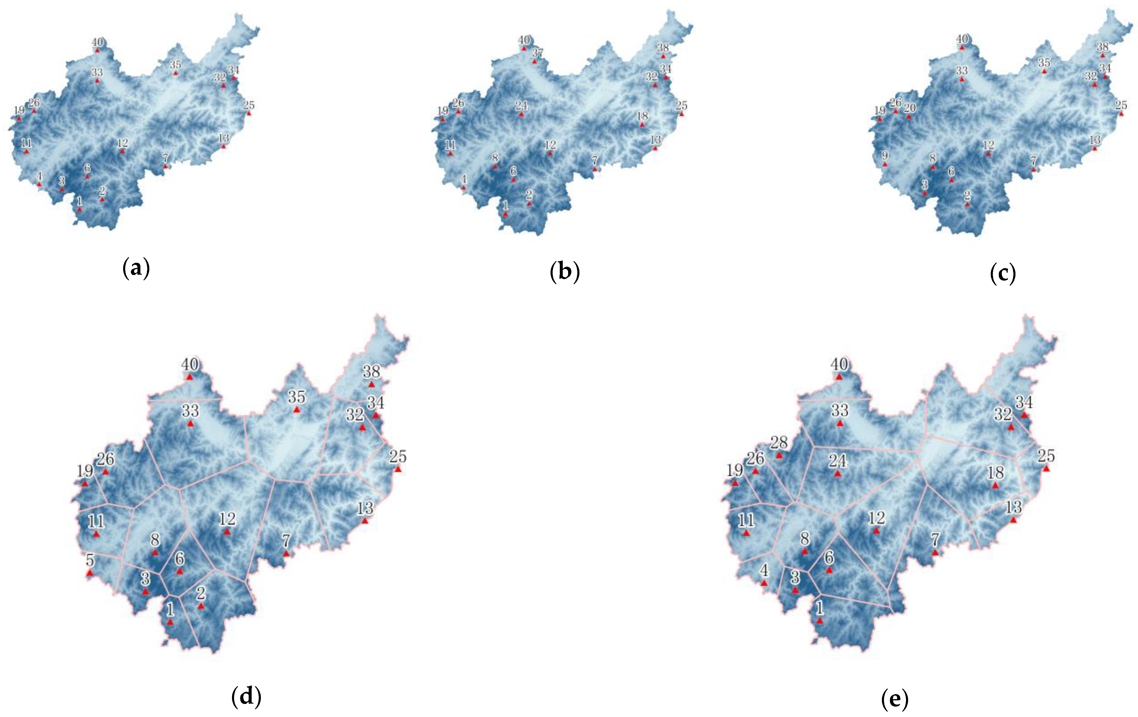
5.1. Comparative Analysis of Rain Gauge Station Network Optimization Design Results
Figure 8 shows the optimized design results of the 40 existing rain gauge stations with the five different types of data. Comparison of Figure 8d,e reveals that the major differences between the two are the decisions regarding stations 24 and 35. In the optimized station networks obtained with any of the three sets of satellite-based data, the schemes with GPM IMERGE Early data and PERSIANN−CCS data retain station 35, whereas that with the GSMaP_NRT data retains station 24. Meanwhile, the optimized scheme with combined satellite-based data retains station 35 and eliminates station 24. Thus, the optimized ranking results obtained with the ground-based precipitation data are more similar to those acquired using the GSMaP_NRT satellite-based daily precipitation deviation data.
Figure 8d,e depict the Thiessen polygons generated by the optimized rain gauge station networks obtained with the three sets of satellite-based data combined and the ground-based precipitation data, respectively. The World Meteorological Organization (WMO) [56] has provided recommendations regarding the rain gauge station density under different terrain and climatic conditions, and it is recommended to set up a station every 600–900 km2. The area covered by each station was determined (Table 3), and Figure 8d shows four stations (stations 7, 12, 33, and 35) with areas greater than 900 km2, whereas Figure 8e shows five such stations (stations 12, 24, 33, 32, and 18). These all occur at relatively low elevations. In general, it is necessary to retain station 35 located in the plain and river valley region, so as to avoid the rain gauge stations being too sparsely distributed. As can be seen from Figure 8d,e, it is clear that rain gauge stations with higher elevations and steep terrain are more likely to be retained, while stations in river valleys and relatively flat areas retain less. In mountainous areas, local climate change is drastic and precipitation is more difficult to capture, resulting in greater precipitation deviations, so stations in mountainous areas are more scarce. In areas with flatter terrain, precipitation deviations vary less between adjacent stations, which are more likely to be discarded. However, this may cause the coverage area (Tyson polygon) of the flat area station to exceed the value recommended by WMO. In this study, 98% of the joint entropy information was preserved and the final station network scheme was determined. One strategy is to increase the threshold of the joint entropy to supplement rain gauge stations, thereby making the coverage area of a single station smaller.
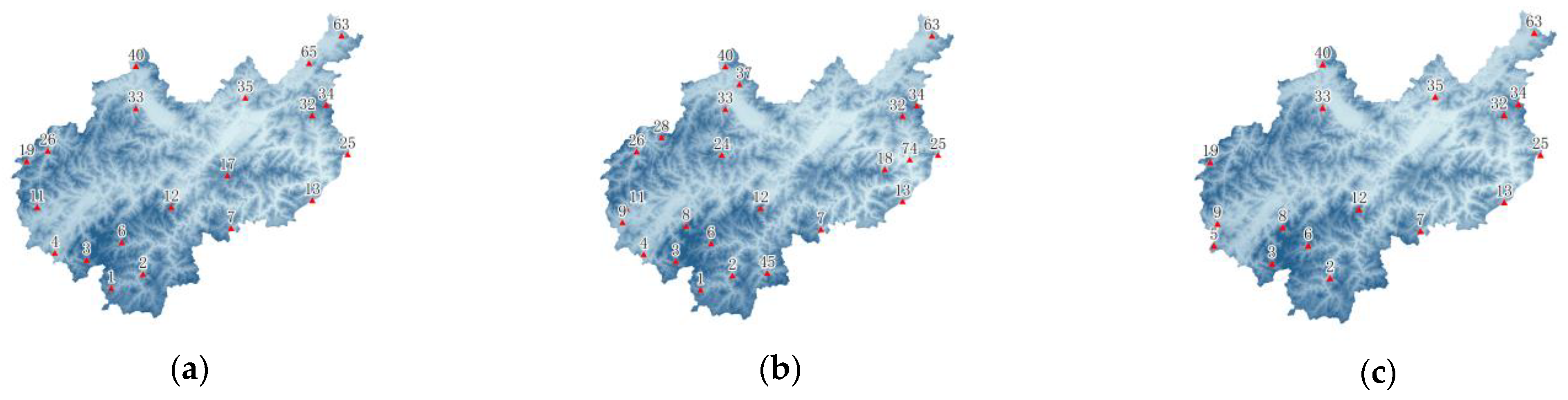
Figure 9 shows the optimized design results of the 75 rain gauge stations with the five types of data. Figure 9d,e reveal that the major differences between the two scenarios are related to stations 63 and 71. As shown in Figure 9a–c, the optimized design schemes obtained with any of the three sets of satellite-based data include station 63 in the station network. In addition, station 71 is present as the first station in the network in Figure 9b. Due to station 71 being located among stations 13, 18, and 25, and the optimization scheme based on the ground-based precipitation data has retained these four stations, there is information redundancy to a certain extent. Station 63 is located at the northeastern edge of the Oujiang River Basin, with no other existing stations in its neighborhood, making it a relatively important station. The optimization schemes based on the three sets of satellite precipitation data combined retain stations 32, 34, and 63 instead of the aforementioned stations 32, 34, and 38 in the northeastern direction, which is more reasonable compared to the optimization scheme obtained from ground-based precipitation data.
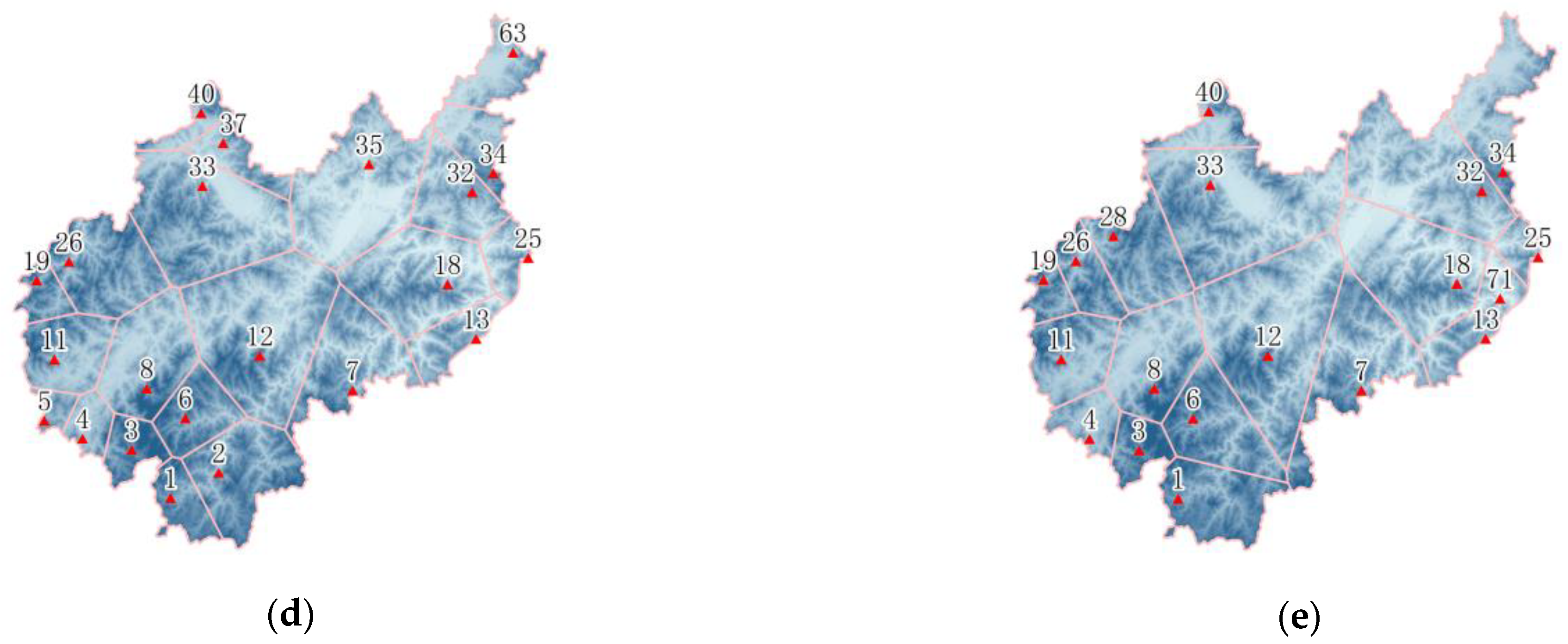
5.2. Comparison of Maximum Joint Information Entropy with Different Rain Gauge Stations
Figure 10a,b show the maximum joint information entropy with different numbers of rain gauge stations obtained by combining the existing stations (stations 1–40) and all the stations (stations 1–75), respectively, using the aforementioned five types of data. The horizontal axis represents the number of rain gauge stations, e.g., 10 indicates any 10 rain gauge stations randomly selected from the set of rain gauge stations, for which the maximum joint information entropy was calculated and plotted. When there is one station, the maximum information entropy of a single station is shown. When there is more than one station, the five curves represent the maximum joint information entropy obtained from the stations retained based on the ranking results shown in Table 1 and Table 2, respectively.
It can be seen from Figure 10 that the information entropies of the first stations obtained with the five types of data do not differ greatly. The differences mainly lie in the changes in the joint information entropy. Among the three sets of satellite precipitation data, PERSIANN−CCS led to the largest joint information entropy due to its relatively high resolution and consequent sensitive daily precipitation deviations between grids. GPM IMERGE Early and GSMaP_NRT have the same spatial resolution, with that of GPM IMERGE Early being slightly better than that of GSMaP_NRT. The joint information entropy obtained with any of the satellite precipitation deviation data, or their combination is significantly greater than that resulting from using the ground-based precipitation data, indicating that satellite precipitation deviation data shows greater changes, a larger total information amount, and a higher degree of distinction in the importance ranking among the stations.
5.3. Analysis of Satellite Precipitation Deviation Interpolation Accuracy
The precipitation deviation obtained by subtracting the ground-based precipitation observation data from the satellite precipitation observation data is called the observed precipitation deviation and indicated by DO. Meanwhile, the precipitation deviation obtained by subtracting the ground-based precipitation interpolation data from the satellite precipitation observation data is called the interpolated precipitation deviation and indicated by DI. In this study, the precipitation deviation data used were the observed DO for stations 1–40 and the interpolated DI for virtual stations 41–75 due to the lack of ground-based precipitation observation data for the virtual stations. However, the precipitation deviation data obtained by Kriging interpolation for these 35 virtual stations has a certain degree of error. Although it is not possible to analyze the accuracy of the interpolated precipitation deviations of the 35 stations directly, it is possible to analyze the overall influence of the Kriging interpolation on the interpolated precipitation deviation data indirectly based on the interpolated precipitation deviation data of the 40 existing stations.
For the convenience of analysis, the GPM IMERGE Early and GSMaP_NRT data were resampled to achieve the same resolution as that of the PERSIANN−CCS data, 0.04° × 0.04°. The resampling adopted nearest neighbor interpolation to avoid affecting the precipitation data accuracy. With the daily precipitation data obtained from the 40 existing rain gauge stations, the gridded daily precipitation data for the entire Oujiang River Basin were obtained by Kriging interpolation at a spatial resolution of 0.04° × 0.04°. The results were subtracted from each of the three sets of satellite precipitation data to obtain three sets of satellite-based gridded daily precipitation deviation data.
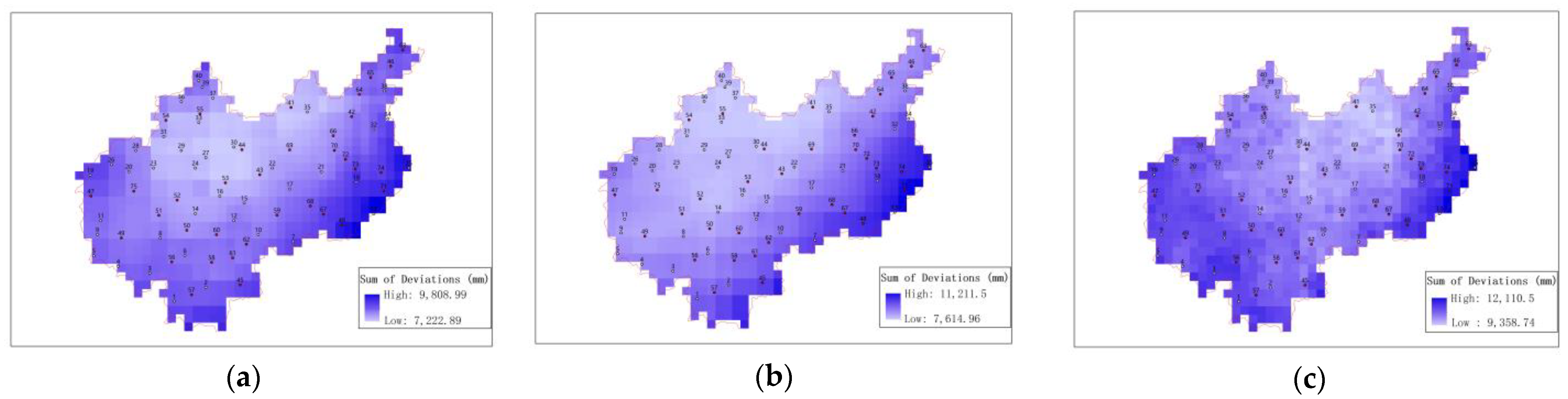
Figure 11 shows the spatial distributions of the cumulative interpolated precipitation deviations obtained by using the three sets of daily satellite precipitation deviation data. It can be seen that GPM IMERGE Early has a cumulative satellite precipitation deviation smaller than those of GSMaP_NRT and PERSIANN−CCS. PERSIANN−CCS has a cumulative satellite precipitation deviation 2000 mm more than that of GPM IMERGE Early, whereas the daily satellite precipitation deviation is 1 mm more than that of the latter. In addition, the cumulative satellite precipitation deviation of GSMaP_NRT changes considerably with a minimum value of 7614.96 mm and maximum value of 11,211.5 mm.
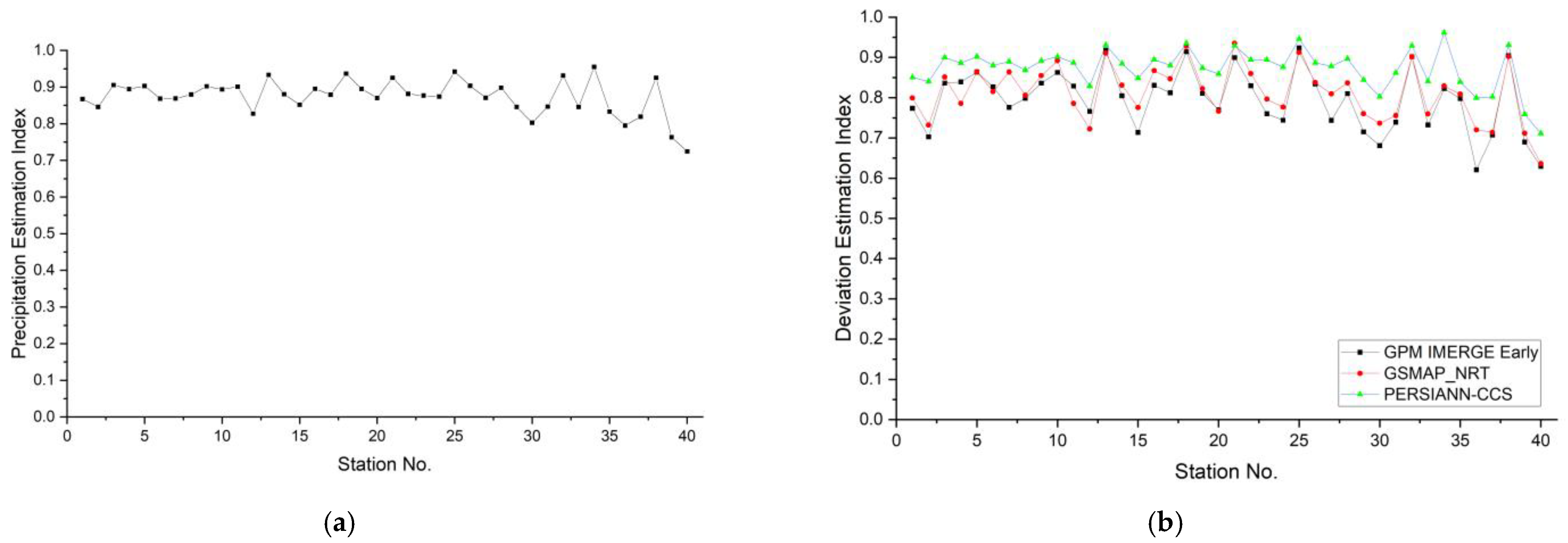
Drawing on the Nash-Sutcliffe efficiency (NSE) coefficient proposed by Nash and Sutcliffe [57] and the goodness of rainfall estimation measure that describes the characteristics of interpolated regional precipitation data sequences proposed by Andréassian et al. [58], this paper proposes the precipitation estimation index (PEI), which evaluates the daily precipitation data accuracy of a single rain gauge station, and the deviation estimation index (DEI), which evaluates the daily precipitation deviation data accuracy. The specific equations are as follows:
In Equations (14) and (15), t is the time step and n is the cumulative amount of time. In this paper, t has units of days, and n represents 2192 days. is the ground-based precipitation observation on day t, is the interpolated amount of ground-based daily precipitation on day t, and is the average amount of ground-based daily precipitation observed at a station. is the deviation between the satellite- and ground-based daily precipitation observations on day t, is the deviation between the satellite-based daily precipitation observation and interpolated ground-based daily precipitation on day t, and is the average satellite precipitation deviation. Similar to the NSE coefficient, both PEI and DEI change between −∞ and 1. If the interpolated precipitation is the same as the observed precipitation, then PEI = 1; if the interpolated precipitation deviation is completely the same as the observed precipitation deviation, then DEI = 1. If the interpolated precipitation is the same as the average observed precipitation, then PEI = 0 and DEI = 0. The closer the values of PEI and DEI to 1, the closer the interpolated data to the observed values. If PEI and DEI are less than 0, the correlation between the interpolated data and observed values is poor.
Figure 12 shows the PEI and DEI curves for the 40 ground-based rain gauge stations. As depicted in Figure 12a, more than 38 stations have PEIs above 0.8, with only stations 39 and 40 having PEIs less than 0.8. As shown in Figure 12b, PERSIANN−CCS has a DEI value close to the PEI value of ground-based rain gauge stations, generally above 0.8. Both GPM IMERGE Early and GSMaP_NRT were influenced by the spatial resolution of the original data and the propagation of interpolated precipitation errors, leading to slightly lower DEIs, which fluctuate around 0.8. Among the 40 rain gauge stations, except for stations 36 and 40, the DEIs of all other stations exceed 0.70.
5.4. Information Entropy Correlation Analysis of Satellite Precipitation Deviation
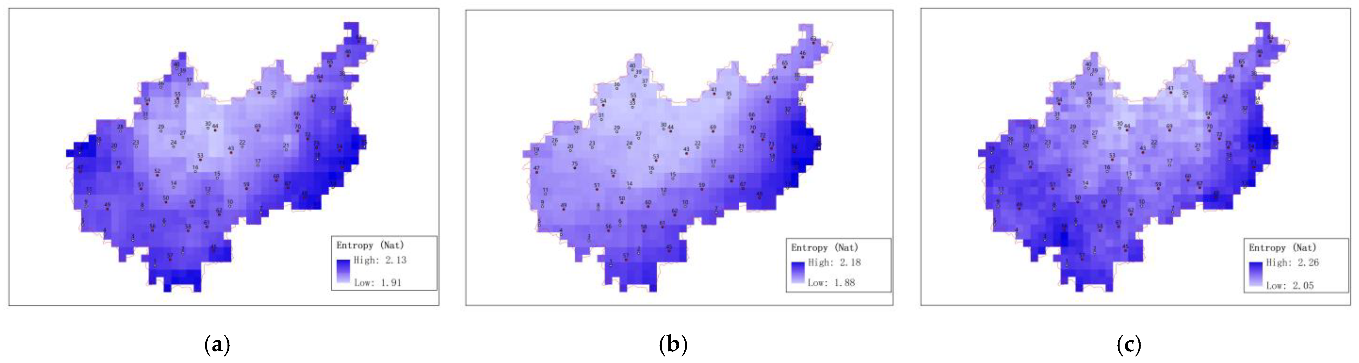
Figure 13 shows the spatial distribution of information entropy throughout the Oujiang River Basin at a resolution of 0.04° × 0.04°, obtained using the three sets of interpolated satellite-based daily precipitation deviation data using Equation (8). It can be seen that GSMaP_NRT has the smallest information entropy among the considered datasets, followed by GPM IMERGE Early, and PERSIANN−CCS has the largest overall information entropy. All three sets of satellite-based data have smaller information entropies in the center and north of the Oujiang River Basin than in other regions, as these areas have relatively low altitudes. In contrast, all three sets of satellite-based data have higher information entropies in the areas close to the eastern and southern edges of the Oujiang River Basin, showing that these areas have greater changes in their precipitation deviations. In the western part of the area, all three sets of satellite-based data exhibit relatively large information entropies. Here, GSMaP_NRT has the smallest information entropy, and the information entropies of GPM IMERGE Early and PERSIANN−CCS show a high degree of consistency.
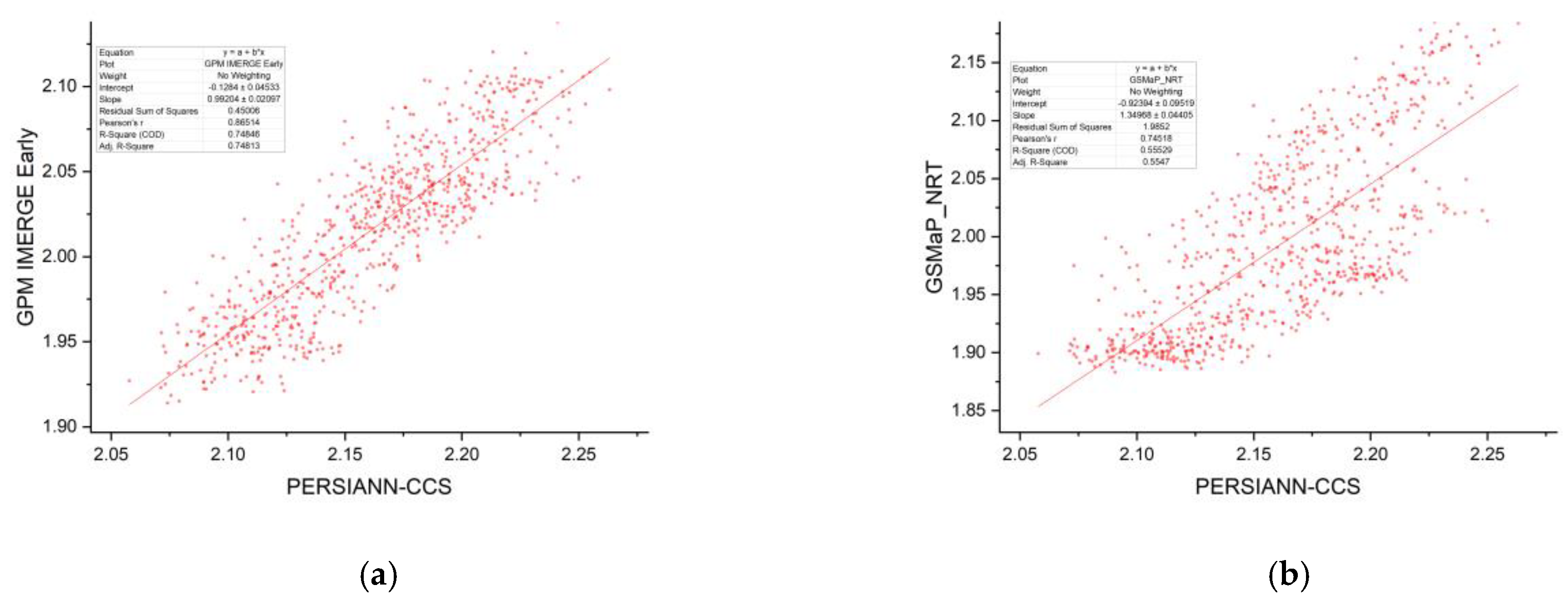
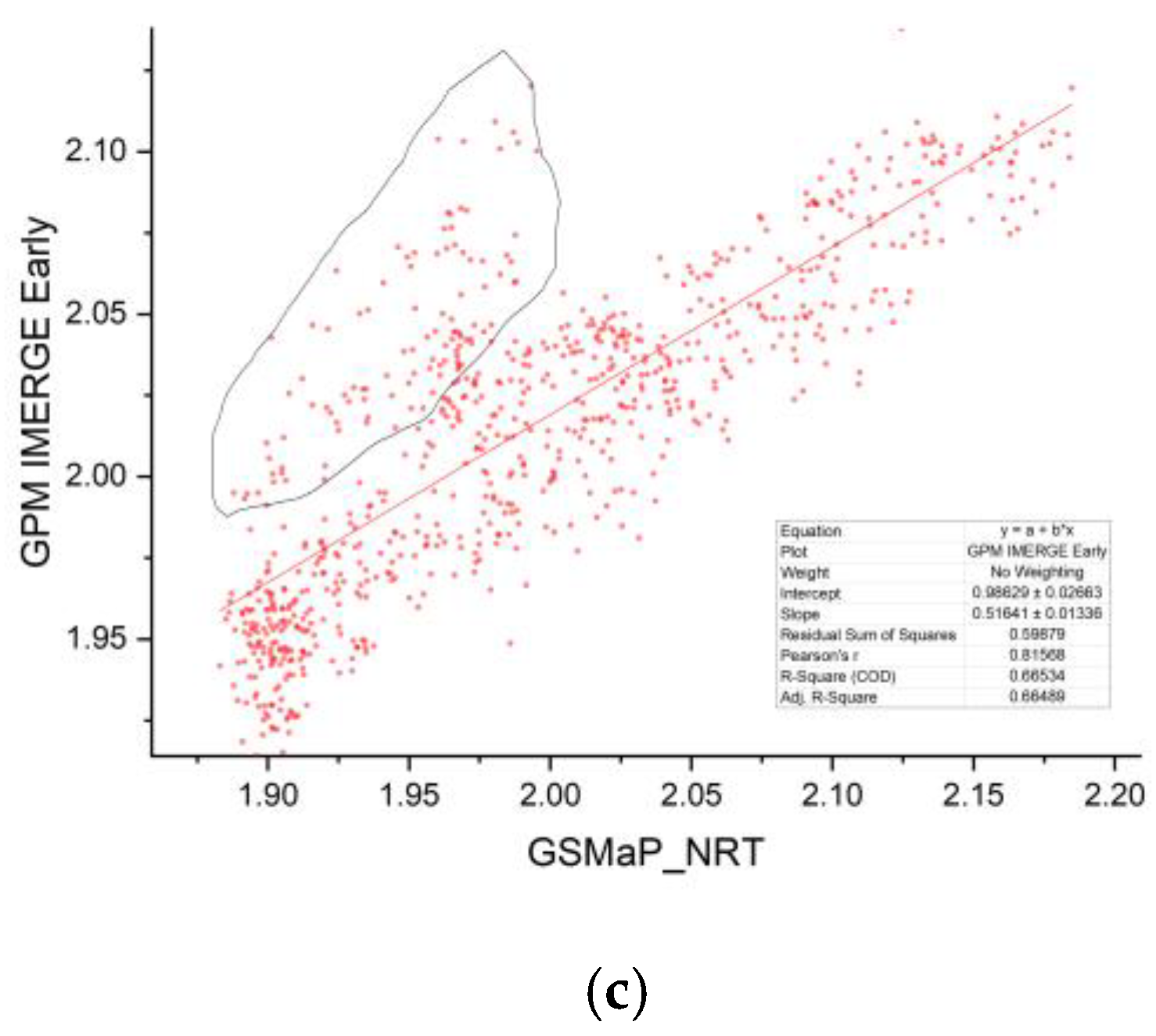
The correlation among the information entropies of the three sets of satellite precipitation deviation data affects the calculation of the joint information entropy and the ranking of the stations. The information entropies of the three sets of satellite precipitation deviation data were thus compared grid by grid, and a scatter plot of the information entropy in pairs was plotted, which was then linearly fitted to evaluate the correlations among the three sets of information entropies. Figure 14a shows that the entropies of PERSIANN−CCS and GPM IMERGE Early exhibit good agreement, followed by that which is between the entropies of PERSIANN−CCS and GSMap_NRT, as shown in Figure 14b. Figure 13 also reveals that PERSIANN−CCS and GPM IMERGE Early are closely correlated according to the spatial distributions of their large and small information entropy values. In contrast, GSMap_NRT shows greater differences between its large and small values, where the large information entropy values are found in the eastern and southern parts of the Oujiang River Basin. Compared with PERSIANN−CCS and GPM IMERGE Early, GSMap_NRT exhibits smaller differences in precipitation deviation in the western part, indicating that GSMap_NRT is more capable of capturing the precipitation in the western part than PERSIANN−CCS and GPM IMERGE Early. The scattered dots enclosed within the line in Figure 14c correspond to those locations in the western part, where the information entropy of the precipitation deviation of GPM IMERGE Early is significantly larger than that of GSMap_NRT. In general, the three sets of satellite-based data show differences in their abilities to capture precipitation in the area to a certain extent. Although the information entropy of the GSMap_NRT precipitation deviation data in the western part is different from that of PERSIANN−CCS and GPM IMERGE Early, a relatively satisfactory station network optimization design scheme can be obtained by combining the three sets of satellite-based data for calculation.
6. Conclusions
Satellite precipitation observation data constitute the most important source of precipitation information besides ground-based precipitation monitoring data and have been increasingly utilized to investigate hydrometeorology, water resources, the global water cycle, and climate change. Data fusion and assimilation by combining satellite precipitation observations and ground-based precipitation monitoring is important for obtaining large-scale high-precision precipitation products. As such, it is essential to develop a well-designed ground-based rain gauge station network with high precision. The existing ground-based rain gauge station network optimization methods are mainly based on rain gauge station precipitation monitoring data, and global station network optimization is performed according to the statistical theory to obtain the smallest error and the principle of maximum entropy. This paper provides a different perspective, evaluating the importance of ground-based rain gauge stations according to satellite precipitation observation data. The conclusions of this study are as follows:
- (1)
- Most of the entropy-based network optimization studies use the rainfall data of rain gauge stations to retain more information and reduce information redundancy. The entropy measure for satellite and ground rainfall deviations is more meaningful and more explanatory. The magnitude of entropy of the rainfall deviations not only expresses the amount of information, but also reflects that some locations are more difficult to measure, and these locations are often affected by topography and geomorphology, and stations should be established here.
- (2)
- Of the three satellite precipitation data, PERSIANN−CCS has the highest spatial resolution. Compared with GPM IMERGE Early and GSMap_NRT, PERSIANN−CCS has more obvious differences in the spatial distribution of precipitation deviation and information entropy, and the calculated joint entropy value is also the largest, which has unique advantages for rain gauge network optimization.
- (3)
- A large number of studies have shown that through various statistical interpolation and machine learning algorithms, satellite precipitation data and ground rainfall data are fused, and the reprocessed data obtained has the advantages of high precision and high resolution. The use of this kind of fused data for rain gauge network optimization is a worthy study in the future.
Author Contributions
H.W. conducted the primary experiments, cartography, and analyzed the results. D.S. provided the original idea for this paper. W.C., Z.H. and Y.X. actively participated throughout the research process and offered data support for this work. All authors have read and agreed to the published version of the manuscript.
Funding
This research was funded by the National Natural Science Foundation of China, grant number 42077438.
Acknowledgments
We would like to thank colleagues in the laboratory for their constructive suggestions. Additionally, we thank the anonymous reviewers and members of the editorial team for their constructive comments.
Conflicts of Interest
The authors declare no conflict of interest.
References
- Sun, Q.; Miao, C.; Duan, Q.; Ashouri, H.; Sorooshian, S.; Hsu, K. A Review of Global Precipitation Data Sets: Data Sources, Estimation, and Intercomparisons. Rev. Geophys. 2018, 56, 79–107. [Google Scholar] [CrossRef] [Green Version]
- Wagner, P.D.; Fiener, P.; Wilken, F.; Kumar, S.; Schneider, K. Comparison and evaluation of spatial interpolation schemes for daily rainfall in data scarce regions. J. Hydrol. 2012, 464–465, 388–400. [Google Scholar] [CrossRef]
- Tiwari, S.; Jha, S.K.; Singh, A. Quantification of Node Importance in Rain gauge station network: Influence of Temporal Resolution and Rain Gauge Density. Sci. Rep. 2020, 10, 9761. [Google Scholar] [CrossRef]
- Xu, H.; Xu, C.; Sælthun, N.R.; Xu, Y.; Zhou, B.; Chen, H. Entropy Theory Based Multi-Criteria Resampling of Rain gauge station networks for Hydrological Modelling—A Case Study of Humid Area in Southern China. J. Hydrol. 2015, 525, 138–151. [Google Scholar] [CrossRef]
- Stosic, T.; Stosic, B.D.; Singh, V.P. Optimizing streamflow monitoring networks using joint permutation entropy. J. Hydrol. 2017, 552, 306–312. [Google Scholar] [CrossRef]
- Leach, J.M.; Kornelsen, K.C.; Samuel, J.; Coulibly, P. Hydrology Network Design Using Streamflow Signatures and Indicators of Hydrologic Alteration. J. Hydrol. 2015, 529, 1350–1359. [Google Scholar] [CrossRef]
- Su, H.; You, G.J. Developing an Entropy-based Model of Spatial Information Estimation and Its Application in the Design of Precipitation Gauge Networks. J. Hydrol. 2014, 519, 3316–3327. [Google Scholar] [CrossRef]
- Li, H.; Wang, D.; Singh, V.P.; Wang, Y.; Wu, J.; Wu, J. Developing an entropy and copula-based approach for precipitation monitoring network expansion. J. Hydrol. 2021, 598, 126366. [Google Scholar] [CrossRef]
- Yeh, H.C.; Chen, Y.C.; Wei, C.; Chen, R.H. Entropy and Kriging approach to Rainfall Network Design. Paddy Water Environ. 2011, 9, 343–355. [Google Scholar] [CrossRef]
- Adhikary, S.K.; Yilmaz, A.G.; Muttil, N. Optimal Design of Rain gauge station network in the Middle Yarra River Catchment, Australia. Hydrol. Process. 2015, 29, 2582–2599. [Google Scholar] [CrossRef]
- Safavi, M.; Siuki, A.K.; Hashemi, S.R. New optimization methods for designing rain stations network using new neural network, election, and whale optimization algorithms by combining the Kriging method. Environ. Monit. Assess. 2021, 193, 4. [Google Scholar] [CrossRef]
- Bárdossy, A.; Pegram, G.G.S. Copula Based Multisite Model for Daily Precipitation Simulation. Hydrol. Earth Syst. Sci. 2009, 13, 2299–2314. [Google Scholar] [CrossRef] [Green Version]
- Vivekanandan, N.; Jagtap, R.S. Evaluation and Selection of Rain gauge station network using Entropy. J. Inst. Eng. 2012, 93, 223–232. [Google Scholar]
- Feki, H.; Mohamed, S.; Cudennec, C.H. Geostatistically based optimization of a precipitation monitoring data network extension: Case of the climatically heterogeneous Tunisia. Hydrol. Res. 2017, 48, 514–541. [Google Scholar] [CrossRef]
- Ali, M.Z.M.; Othman, F. Rain gauge station network optimization in a tropical urban area by coupling cross-validation with the geostatistical technique. Hydrol. Sci. J. 2018, 63, 474–491. [Google Scholar] [CrossRef]
- Xu, H.; Xu, C.Y.; Chen, H.; Zhang, Z.; Li, L. Assessing the Influence of Rain gauge Distribution on Hydrological Model Performance in a Humid Region of China. J. Hydrol. 2013, 505, 1–12. [Google Scholar] [CrossRef]
- Cetinkaya, C.P.; Harmancioglu, N.B. Reduction of Streamflow Monitoring Networks by a Reference Point Approach. J. Hydrol. 2014, 512, 263–273. [Google Scholar] [CrossRef]
- Kar, A.K.; Lohani, A.K.; Goel, N.K.; Roy, G.P. Rain gauge station network Design for Flood Forecasting Using Multi-Criteria Decision Analysis and Clustering Techniques in Lower Mahanadi River Basin, India. J. Hydrol. 2015, 4, 313–332. [Google Scholar]
- Fahle, M.; Hohenbrink, T.L.; Dietrich, O.; Lischeid, G. Temporal Variability of the Optimal Monitoring Setup Assessed Using Information Theory. Water Resour. Res. 2015, 51, 7723–7743. [Google Scholar] [CrossRef] [Green Version]
- Chacon-Hurtado, J.C.; Alfonso, L.; Solomatine, D.P. Rainfall and Streamflow Sensor Network Design: A Review of Application, Classification, and a Proposed Framework. Hydrol. Earth Syst. Sci. 2017, 21, 3071–3091. [Google Scholar] [CrossRef] [Green Version]
- Keum, J.; Coulibaly, P. Information Theory-based Decision Support System for Integrated Design of Multi-variable Hydrometric Network. Water Resour. Res. 2017, 53, 6239–6259. [Google Scholar] [CrossRef]
- Keum, J.; Kornelsen, K.C.; Leach, J.M.; Coulibaly, P. Entropy Applications to Water Monitoring Network Design: A Review. Entropy 2017, 19, 613. [Google Scholar] [CrossRef]
- Yuan, Y.; Yang, X.; Chen, L.; Yuan, X.; Dong, H.; Yu, Y. Optimization of The Basin Hydrologic Network Based on Multi-objective Criteria. J. Hohai Univ. Nat. Sci. 2019, 47, 102–107. [Google Scholar]
- Wang, W.; Wang, D.; Singh, V.P.; Wang, Y.; Wu, J.; Zhang, J.; Liu, J.; Zou, Y.; He, R.; Meng, D. Evaluation of Information Transfer and Data Transfer Models of Rain gauge station network Design Based on Information Entropy. Environ. Res. 2019, 178, 108686. [Google Scholar] [CrossRef]
- Li, C.; Singh, V.P.; Mishra, A.K. Entropy Theory-based Criterion for Hydrometric Network Evaluation and Design: Maximum Information Minimum Redundancy. Water Resour. Res. 2012, 48, W05521. [Google Scholar] [CrossRef]
- Alfonso, L.; Lobbrecht, A.; Price, R. Optimization of Water Level Monitoring Network in Polder Systems Using Information Theory. Water Resour. Res. 2010, 46, W12553. [Google Scholar] [CrossRef]
- Husain, T. Hydrologic Uncertainty Measure and Network Design. Water Resour. Bull. 1989, 25, 527–534. [Google Scholar] [CrossRef]
- Meng, C.; Mo, X.; Liu, S.; Hu, S. Extensive Evaluation of IMERGE Precipitation for Both Liquid and Solid in Yellow River Source Region. Atmos. Res. 2021, 256, 105570. [Google Scholar] [CrossRef]
- Su, J.; Lü, H.; Zhu, Y.; Gui, Y.; Wang, X. Evaluating the hydrological utility of latest IMERGE Products over the Upper Huaihe River Basin, China. Atmos. Res. 2019, 225, 17–29. [Google Scholar] [CrossRef]
- Tang, G.; Ma, Y.; Long, D.; Zhong, L.; Hong, Y. Evaluation of GPM Day-1 IMERGE and TMPA Version-7 Legacy Products over Mainland China at multiple Spatiotemporal Scales. J. Hydrol. 2016, 533, 152–167. [Google Scholar] [CrossRef]
- Lu, X.; Tang, G.; Wang, X.; Liu, Y.; Wei, M.; Zhang, Y. The Development of a Two-Step Merging and Downscaling Method for Satellite Precipitation Products. Remote Sens. 2020, 12, 398. [Google Scholar] [CrossRef] [Green Version]
- Yan, X.; Chen, H.; Tian, B.; Sheng, S.; Wang, J.; Kim, J. A Downscaling-Merging Scheme for Improving Daily Spatial Precipitation Estimates Based on Random Forest and Cokriging. Remote Sens. 2021, 13, 2040. [Google Scholar] [CrossRef]
- Jia, S.; Zhu, W.; Lu, A.; Yan, T. A Statistical Spatial Downscaling Algorithm of TRMM Precipitation Based on NDVI and DEM in the Qaidam Basin of China. Remote Sens. Environ. 2011, 115, 3069–3079. [Google Scholar] [CrossRef]
- Zhang, Q.; Shi, P.; Singh, V.P.; Fan, K.; Huang, J. Spatial Downscaling of TRMM-based Precipitation Data Using Vegetative Response in Xinjiang, China. Int. J. Climatol. 2016, 37, 3895–3909. [Google Scholar] [CrossRef]
- Chen, Y.; Huang, J.; Sheng, S.; Mansaray, L.R.; Liu, Z.; Wu, H.; Wang, X. A New Downscaling-Integration Framework for High-Resolution Monthly Precipitation Estimates: Combining Rain Gauge Observations, Satellite-Derived Precipitation Data and Geographical Ancillary Data. Remote Sens. Environ. 2018, 214, 154–172. [Google Scholar] [CrossRef]
- Dai, Q.; Bray, M.; Zhuo, L.; Islam, T.; Han, D.W. A Scheme for Rain Gauge Station Network Design Based on Remotely-sensed Rainfall Measurements. J. Hydrometeorol. 2017, 18, 363–379. [Google Scholar] [CrossRef]
- Yeh, H.C.; Chen, Y.C.; Chang, C.H.; Ho, C.H.; Wei, C. Rainfall Network Optimization Using Radar and Entropy. Entropy 2017, 19, 553. [Google Scholar] [CrossRef] [Green Version]
- Morsy, M.; Taghizadeh-Mehrjardi, R.; Michaelides, S.; Scholten, T.; Dietrich, P.; Schmidt, K. Optimization of Rain Gauge Networks for Arid Regions Based on Remote Sensing Data. Remote Sens. 2021, 13, 4243. [Google Scholar] [CrossRef]
- Shannon, C.E. A Mathematical Theory of Communication. Bell Syst. Tech. J. 1948, 27, 623–656. [Google Scholar] [CrossRef]
- Keum, J.; Coulibaly, P.; Razavi, T.; Tapspba, D.; Gobena, A.; Weber, F.; Pietroniro, A. Application of SNODAS and Hydrologic Models to Enhance Entropy-based Snow Monitoring Network Design. J. Hydrol. 2018, 561, 688–701. [Google Scholar] [CrossRef]
- Ridolfi, E.; Montesarchio, V.; Russo, F.; Napolitano, F. An entropy Approach for Evaluating the Maximum Information Content Achievable by an Urban Rainfall Network. Nat. Hazards Earth Syst. Sci. 2011, 11, 2075–2083. [Google Scholar] [CrossRef] [Green Version]
- Awadallah, A.G. Selecting Optimum Locations of Rainfall Stations Using Kriging and Entropy. Int. J. Energy Environ. Eng. 2012, 12, 36–41. [Google Scholar]
- Mahmoudi-Meimand, H.; Nazif, S.; Abbaspour, R.A.; Sabokbar, H.F. An Algorithm for Optimisation of a Rain gauge station network Based on Geostatistics and Entropy Concepts Using GIS. J. Spat. Sci. 2016, 61, 233–252. [Google Scholar] [CrossRef]
- Papadopoulou, M.; Raphael, B.; Smith, I.F.C.; Sekhar, C. Hierarchical sensor placement using joint entropy and the effect of modeling error. Entropy 2014, 16, 5078–5101. [Google Scholar] [CrossRef]
- Bertola, N.J.; Papadopoulou, M.; Vernay, D.; Smith, I.F.C. Optimal multi-type sensor placement for structural identification by static-load testing. Sensors 2017, 17, 2904. [Google Scholar] [CrossRef] [Green Version]
- Papadopoulou, M.; Raphael, B.; Smith IF, C.; Sekhar, C. Optimal Sensor Placement for Time-Dependent Systems: Application to Wind Studies around Buildings. J. Comput. Civil. Eng. 2016, 30, 4015024. [Google Scholar] [CrossRef] [Green Version]
- Hu, Z.; Chen, W.; Chen, B.; Tan, D.; Zhang, Y.; Shen, D. Robust Hierarchical Sensor Optimization Placement Method for Leak Detection in Water Distribution System. Water Resour. Manag. 2021, 35, 3995–4008. [Google Scholar] [CrossRef]
- Chen, Y.C.; Wei, C.; Yeh, H.C. Rainfall network design using kriging and entropy. Hydrol. Process. 2008, 22, 340–346. [Google Scholar] [CrossRef]
- Wei, C.; Yeh, H.C.; Chen, Y.C. Spatialtemporal Scaling Effect on Rainfall Networks Design Using Entropy. Entropy 2014, 16, 4626–4627. [Google Scholar] [CrossRef] [Green Version]
- Xu, P.; Wang, D.; Singh, V.P.; Wang, Y.; Wu, J.; Wang, L. A kriging and entropy-based approach to rain gauge network design. Environ. Res. 2018, 161, 61–75. [Google Scholar] [CrossRef]
- Habib, E.; Henschke, A.; Adler, R.F. Evaluation of TMPA satellite-based research and real-time rainfall estimates during six tropical-related heavy rainfall events over Louisiana, USA. Atmos. Res. 2009, 94, 373–388. [Google Scholar] [CrossRef]
- Liu, Z. Comparison of precipitation estimation between Version 7 3-hourly TRMM Multi-Satellite Precipitation Analysis (TMPA) near-real-time and research products. Atmos. Res. 2015, 153, 119–133. [Google Scholar] [CrossRef] [Green Version]
- Hénin, R.; Liberato, M.; Ramos AGouveia, C. Assessing the Use of Satellite-Based Estimates and High-Resolution Precipitation Datasets for the Study of Extreme Precipitation Events over the lberian Peninsula. Water 2018, 10, 1688. [Google Scholar] [CrossRef] [Green Version]
- Yong, B.; Chen, B.; Gourley, J.J.; Ren, L.; Hong, Y.; Chen, X.; Wang, W.; Chen, S.; Gong, L. Intercomparison of the Version-6 and Version-7 TMPA precipitation products over high and low latitudes basins with independent gauge networks: Is the newer version better in both real-time and post-real-time analysis for water resources and hydrologic extremes? J. Hydrol. 2014, 508, 77–87. [Google Scholar]
- Wu, H.; Chen, Y.; Chen, X.; Liu, M.; Gao, L.; Deng, H. A New Approach for Optimizing Rain gauge station networks: A Case Study in the Jinjiang Basin. Water 2020, 12, 2252. [Google Scholar] [CrossRef]
- WMO (World Meteorological Organization). Guide to Hydrometeorological Practices, Volume I: Hydrology—From Measurement to Hydrological Information (WMO Publication 168, Vol. I); World Meteorological Organization: Geneva, Switzerland, 2008.
- Nash, J.E.; Sutcliffe, J.V. River flow forecasting through conceptual models. Part I—A discussion of principles. J. Hydrol. 1970, 370, 139–154. [Google Scholar] [CrossRef]
- Andréassian, V.; Perrin, C.; Michel, C.; Usart-Sanchez, I.; Lavabre, J. Impact of imperfect rainfall knowledge on the efficiency and the parameters of watershed models. J. Hydrol. 2001, 250, 206–223. [Google Scholar] [CrossRef]
Figure 1.
Flow chart of rain gauge station network optimization.

Figure 2.
Schematic diagrams of information entropy of rain gauge stations and joint information entropy: (a) Information entropy of rain gauge stations X, Y, and Z; (b) Joint information entropy between the three stations when the degree of redundancy is low; (c) Joint information entropy between the three stations when the degree of redundancy is high.

Figure 3.
Schematic diagram of joint information entropy calculated using layer-by-layer algorithm based on satellite-observed precipitation deviations (a, b and c are three different precipitation deviation values for different days).
Figure 3.
Schematic diagram of joint information entropy calculated using layer-by-layer algorithm based on satellite-observed precipitation deviations (a, b and c are three different precipitation deviation values for different days).

Figure 4.
Oujiang River Basin and rain gauge station distribution.

Figure 5.
Daily precipitation data series at stations 1 and 75 from 1 January 2015–31 December 2020.
Figure 5.
Daily precipitation data series at stations 1 and 75 from 1 January 2015–31 December 2020.

Figure 6.
Spatial distributions of three sets of satellite precipitation data obtained for Oujiang River Basin on 16 July 2020. (a) GPM IMERGE Early; (b) GSMaP_NRT; (c) PERSIANN−CCS.
Figure 6.
Spatial distributions of three sets of satellite precipitation data obtained for Oujiang River Basin on 16 July 2020. (a) GPM IMERGE Early; (b) GSMaP_NRT; (c) PERSIANN−CCS.

Figure 7.
Daily precipitation deviations between three sets of satellite precipitation data and ground-based precipitation data observed at rain gauge station 1.
Figure 7.
Daily precipitation deviations between three sets of satellite precipitation data and ground-based precipitation data observed at rain gauge station 1.

Figure 8.
Optimized design results for 40 existing rain gauge stations with five types of data. (a) optimized station network with GPM IMERGE Early data; (b) optimized station network with GSMaP_NRT data; (c) optimized station network with PERSIANN−CCS data; (d) optimized station network with the three sets of satellite-based data combination; (e) optimized station network with rain gauge data.

Figure 9.
Optimized design results of 75 rain gauge stations with five types of data. (a) optimized station network with GPM IMERGE Early data; (b) optimized station network with GSMaP_NRT data; (c) optimized station network with PERSIANN−CCS data; (d) optimized station network with the three sets of satellite-based data combination; (e) optimized station network with rain gauge data.


Figure 10.
Maximum joint information entropy with different combinations of rain gauge stations. (a) With existing rain gauge stations (stations 1–40); (b) With 40 existing rain gauge stations and 35 virtual rain gauge stations (stations 1–75).
Figure 10.
Maximum joint information entropy with different combinations of rain gauge stations. (a) With existing rain gauge stations (stations 1–40); (b) With 40 existing rain gauge stations and 35 virtual rain gauge stations (stations 1–75).

Figure 11.
Spatial distributions of cumulative precipitation deviations for three sets of satellite-based data. (a) GPM IMERGE Early; (b) GSMaP_NRT; (c) PERSIANN−CCS.
Figure 11.
Spatial distributions of cumulative precipitation deviations for three sets of satellite-based data. (a) GPM IMERGE Early; (b) GSMaP_NRT; (c) PERSIANN−CCS.

Figure 12.
PEIs and DEIs of 40 ground-based rain gauge stations. (a) Rain gauge PEI; (b) DEIs of three satellites.
Figure 12.
PEIs and DEIs of 40 ground-based rain gauge stations. (a) Rain gauge PEI; (b) DEIs of three satellites.

Figure 13.
Spatial distributions of information entropies of three sets of interpolated satellite-based daily precipitation deviation data. (a) GPM IMERGE Early; (b) GSMaP_NRT; (c) PERSIANN−CCS.
Figure 13.
Spatial distributions of information entropies of three sets of interpolated satellite-based daily precipitation deviation data. (a) GPM IMERGE Early; (b) GSMaP_NRT; (c) PERSIANN−CCS.

Figure 14.
Spatial distribution correlation analysis of information entropies obtained from three sets of satellite precipitation deviation data. (a) PERSIANN−CCS and GPM IMERGE Early; (b) PERSIANN-CCS and GSMaP_NRT; (c) GSMaP_NRT and GPM IMERGE Early.
Figure 14.
Spatial distribution correlation analysis of information entropies obtained from three sets of satellite precipitation deviation data. (a) PERSIANN−CCS and GPM IMERGE Early; (b) PERSIANN-CCS and GSMaP_NRT; (c) GSMaP_NRT and GPM IMERGE Early.


Table 1.
Optimized ranking results of the 40 existing rain gauge stations in the network.
| Precipitation Products | Number of Retained Stations | Optimized Ranking Results |
|---|---|---|
| GPM | 17 | 12, 19, 25, 40, 1, 34, 7, 11, 2, 33, 35, 32, 26, 13, 6, 4, 3, 17, 9, 10, 18, 36, 24, 22, 38, 28, 8, 30, 5, 16, 14, 15, 31, 37, 27, 20, 21, 23, 29, 39 |
| GSMaP | 19 | 25, 12, 1, 37, 34, 13, 11, 32, 6, 4, 40, 2, 26, 18, 24, 19, 38, 8, 7, 5, 33, 28, 29, 35, 3, 17, 21, 16, 10, 30, 9, 14, 15, 22, 31, 23, 20, 27, 36, 39 |
| PERSIANN | 18 | 25, 3, 40, 12, 34, 7, 19, 9, 6, 13, 33, 8, 32, 26, 2, 38, 20, 35, 30, 5, 1, 24, 18, 28, 36, 17, 22, 4, 14, 37, 10, 21, 23, 31, 29, 39, 11, 16, 27, 15 |
| Combination | 19 | 12, 25, 40, 1, 34, 19, 7, 11, 13, 6, 32, 33, 8, 26, 2, 5, 38, 35, 3, 18, 37, 24, 4, 28, 17, 30, 22, 10, 14, 20, 9, 36, 16, 21, 29, 15, 31, 23, 27, 39 |
| Rain Gauge | 19 | 12, 25, 19, 1, 40, 13, 34, 8, 7, 33, 11, 3, 32, 6, 26, 24, 18, 4, 28, 2, 5, 17, 29, 38, 35, 14, 22, 37, 10, 9, 30, 15, 23, 31, 16, 39, 27, 20, 21, 36 |
Table 2.
Optimized ranking results of 75 rain gauge stations in the network (showing only the top 40 stations).
Table 2.
Optimized ranking results of 75 rain gauge stations in the network (showing only the top 40 stations).
| Precipitation Products | Number of Retained Stations | Optimized Ranking Results |
|---|---|---|
| GPM | 20 | 12, 19, 25, 40, 1, 34, 7, 11, 63, 2, 32, 33, 35, 13, 6, 26, 4, 65, 3, 17, 9, 10, 67, 18, 24, 36, 22, 28, 8, 30, 16, 61, 5, 14, 15, 60, 47, 42, 74, 54 |
| GSMaP | 25 | 71, 12, 1, 34, 40, 25, 8, 32, 9, 7, 63, 33, 3, 13, 11, 45, 6, 4, 37, 26, 2, 18, 74, 24, 28, 47, 38, 57, 17, 29, 5, 35, 16, 65, 10, 68, 30, 14, 15, 22 |
| PERSIANN | 19 | 25, 3, 40, 12, 34, 7, 19, 9, 6, 13, 33, 8, 63, 32, 26, 2, 37, 5, 35, 20, 30, 62, 18, 42, 1, 24, 4, 17, 14, 28, 54, 22, 21, 16, 36, 31, 46, 66, 10, 39 |
| Combination | 22 | 12, 25, 40, 1, 34, 19, 7, 11, 63, 13, 6, 32, 33, 8, 2, 26, 5, 35, 18, 3, 37, 4, 24, 65, 28, 17, 74, 45, 30, 22, 9, 14, 16, 57, 20, 42, 10, 67, 62, 36 |
| Rain Gauge | 20 | 71, 12, 19, 1, 34, 40, 7, 8, 25, 13, 11, 33, 3, 6, 26, 4, 18, 32, 24, 28, 2, 5, 17, 29, 38, 14, 22, 35, 37, 10, 9, 30, 15, 23, 31, 16, 39, 27, 73, 20 |
Table 3.
Comparison of station coverage area under the optimization of 40 and 75 stations.
| Optimization of 40 Rain Gauge Stations | Optimization of 75 Rain Gauge Stations | ||||||
|---|---|---|---|---|---|---|---|
| Satellite Combination | Rain Gauge | Satellite Combination | Rain Gauge | ||||
| StationID | Area (km2) | StationID | Area (km2) | StationID | Area (km2) | StationID | Area (km2) |
| 12 | 1604.40 | 12 | 1333.27 | 12 | 1628.26 | 12 | 1769.77 |
| 33 | 1594.85 | 32 | 1298.03 | 33 | 1413.78 | 33 | 1697.74 |
| 35 | 1539.17 | 18 | 1291.90 | 35 | 1359.07 | 32 | 1276.79 |
| 7 | 971.98 | 33 | 1226.63 | 18 | 1035.34 | 18 | 1235.89 |
| 8 | 865.63 | 24 | 1177.67 | 8 | 817.27 | 7 | 940.44 |
| 2 | 814.46 | 7 | 880.68 | 2 | 808.73 | 8 | 794.31 |
| 13 | 791.39 | 34 | 735.51 | 26 | 800.16 | 6 | 724.06 |
| 26 | 769.26 | 6 | 720.30 | 7 | 785.44 | 34 | 706.19 |
| 32 | 748.61 | 1 | 694.81 | 32 | 563.60 | 28 | 678.17 |
| 38 | 661.76 | 8 | 690.43 | 11 | 547.05 | 1 | 668.80 |
| 11 | 543.84 | 11 | 585.88 | 6 | 444.57 | 11 | 571.80 |
| 6 | 452.37 | 28 | 465.00 | 63 | 378.58 | 26 | 340.52 |
| 3 | 356.45 | 26 | 349.20 | 34 | 353.50 | 40 | 315.66 |
| 40 | 310.05 | 13 | 344.95 | 13 | 344.95 | 4 | 286.75 |
| 1 | 291.50 | 40 | 317.85 | 1 | 298.99 | 13 | 272.57 |
| 25 | 281.37 | 4 | 282.43 | 37 | 293.44 | 3 | 266.49 |
| 5 | 207.06 | 3 | 268.75 | 3 | 268.75 | 71 | 202.88 |
| 19 | 194.09 | 25 | 236.27 | 25 | 236.27 | 19 | 194.24 |
| 34 | 104.91 | 19 | 203.59 | 4 | 208.68 | 25 | 160.09 |
| 19 | 203.59 | ||||||
| 40 | 200.55 | ||||||
| 5 | 112.58 | ||||||
Publisher’s Note: MDPI stays neutral with regard to jurisdictional claims in published maps and institutional affiliations. |
© 2022 by the authors. Licensee MDPI, Basel, Switzerland. This article is an open access article distributed under the terms and conditions of the Creative Commons Attribution (CC BY) license (https://creativecommons.org/licenses/by/4.0/).
Share and Cite
MDPI and ACS Style
Wang, H.; Chen, W.; Hu, Z.; Xu, Y.; Shen, D. Optimal Rain Gauge Network Design Aided by Multi-Source Satellite Precipitation Observation. Remote Sens. 2022, 14, 6142. https://doi.org/10.3390/rs14236142
AMA Style
Wang H, Chen W, Hu Z, Xu Y, Shen D. Optimal Rain Gauge Network Design Aided by Multi-Source Satellite Precipitation Observation. Remote Sensing. 2022; 14(23):6142. https://doi.org/10.3390/rs14236142
Chicago/Turabian StyleWang, Helong, Wenlong Chen, Zukang Hu, Yueping Xu, and Dingtao Shen. 2022. "Optimal Rain Gauge Network Design Aided by Multi-Source Satellite Precipitation Observation" Remote Sensing 14, no. 23: 6142. https://doi.org/10.3390/rs14236142
Note that from the first issue of 2016, this journal uses article numbers instead of page numbers. See further details here.