
A Motion-Correction Method for Turbulence Estimates from Floating Lidars

1
DTU Wind and Energy Systems, Technical University of Denmark, 4000 Roskilde, Denmark
2
RLC OWS OC, Equinor ASA, 5020 Bergen, Norway
*
Author to whom correspondence should be addressed.
Remote Sens. 2022, 14(23), 6065; https://doi.org/10.3390/rs14236065
Submission received: 2 September 2022
/
Revised: 18 November 2022
/
Accepted: 27 November 2022
/
Published: 30 November 2022
(This article belongs to the Special Issue Feature Papers of Section Atmosphere Remote Sensing)
Abstract
:Estimates of atmospheric turbulence performed by both fixed and floating vertically profiling, conically scanning wind lidars are affected by the measurement volume and turbulence structure, among others. We study this phenomenon by simulating the lidar measurements within synthetic fields of atmospheric turbulence. We use the simulations’ framework to assess the impact of buoy motions on turbulence estimation. Simulation results show that the buoy’s translational motions impact turbulence estimates the most. We also apply the simulation framework to analyze measurements from a floating lidar measuring nearby an offshore meteorological mast for a period of six months. The analysis of measurements is presented both without and with motion compensation. In general, we find from both simulations and measurements that the buoy motions do not impact the mean horizontal wind speed significantly, in agreement with previous studies. However, both simulations and measurements show that the standard deviation of the horizontal velocity is overestimated by the floating lidar. When we correct the measurements based on compensation factors derived from the simulations, the mean bias of the horizontal wind speed standard deviation changes from 18–19% to 5–21%, with large reductions at the first four heights closest to the surface and a slight increase at the highest vertical level.
1. Introduction
It has been more than a decade since the first floating wind profiling lidars (hereafter simply referred to as floating lidars) were introduced. Floating lidar’s main objective is to help the wind energy industry and research community assess offshore wind resources. Offshore meteorological masts are very expensive to install and maintain. Thus, floating lidars have become the new standard for offshore wind measurements. However, until now, floating lidars have primarily been used to measure mean wind speed and direction, as these are the two critical parameters to make wind farm projects profitable. Other parameters for turbine siting are still not well explored from floating lidar measurements.
A still recent and well-elaborated technology status of floating lidars can be found in Gottschall et al. [1]. As they pointed out, one of the critical aspects of floating lidars is related to the motion of the buoy/system. The motion of a floating lidar has an effect on both the mean wind speed and turbulence measurements. Experimental campaigns using floating lidars have shown that their computed 10-min mean winds, when compared to either cup anemometer measurements on masts or fixed lidars nearby the floating lidar, are very good. Highly accurate and precise mean winds, with a nearly zero mean bias and coefficients of determination close to unity even without accounting/compensating for the buoy’s motion have been previously found [2,3]. A theoretical investigation of the nearly zero bias on the mean was performed by Kelberlau and Mann [4]. Similar agreement is found for the 10-min wind direction estimations. As mentioned by Kelberlau et al. [5], for estimates of the wind direction, one can compensate the measured wind direction with a simple yaw correction at the 10-min level [1].
However, Gottschall et al. [2] already showed that turbulence measurements from a floating lidar installed close to the FINO1 offshore platform in the German Bight were heavily impacted by the buoy’s motion. They showed a clear dependency of the error in the turbulence intensity (TI) estimates, given as the difference between the TI from the floating lidar and the TI from the cup anemometer on the mast at the platform, as a function of the significant wave height. Thus, the estimates of TI require some sort of motion compensation. Due to the buoy’s motion, the measured velocity fluctuations are generally larger than those of fixed wind lidars, cup or sonic anemometers. The difference depends on the amplitude and period of the buoy’s motion.
One way to compensate for the buoy’s motion is hardware-based. The compensation could be passive, e.g., gimbal- or spring-like mounting, or active, i.e., using the motion of the buoy to mechanically ‘correct’ its position [1,6]. Current hardware-based methods increase both the cost and the complexity of floating lidars. In addition, they cannot compensate for large motions of the buoy.
The other way for compensating for the buoy motion is to perform either online- or post-processing of the lidar and/or buoy motion signals. Window averaging on the horizontal velocity time series was proposed by Gutiérrez et al. [7] to low-pass filter the lidar signal. This method can be applied when the lidar velocity estimate is at a higher frequency than that of the motion of the buoy. For a continuous wave (CW) lidar focusing sequentially at several heights (focused height is where the intensity of the light is highest) or a ‘slow’ pulsed system, this is hardly the case as the periods of buoy motions are below 4–5 s. Gutiérrez-Antuñano et al. [8] simulated the velocity azimuth display (VAD) scanning configuration performed by most floating lidars on a simplistic flow. They compensated the error on the turbulence statistics by accounting for the effect of the amplitude and period of the buoy’s motion. They showed that the error in TI estimation can be reduced from 38% to 4%.
The straightforward way to account for the buoy’s motion is to compensate directly the radial velocity within the VAD scan with the information from the signals of the buoy’s motion [5,9]. This method has shown promising results in terms of TI estimation, but it is cumbersome to record radial velocities and high-frequency buoy signals, as the amount of data heavily increases and, for floating lidars in particular, this is an important issue.
Here we present a different approach to compensate for the buoy motion because we do not have access to radial velocity measurements. We immerse a floating lidar within atmospheric turbulence boxes, i.e., randomly generated realizations of synthetic fields of atmospheric turbulence, and simulate the lidar measurements while subjected to the buoy’s motion. Thus, we can study the effect of different rotational and translational motions on the characteristics of the reconstructed wind field. Moreover, we assess the impact of the correction by comparing the results to measurements from an ideal sonic anemometer on a fixed platform. An advantage of our method compared to previous work is that we can determine the effect of the buoy’s motion on each radial velocity measurement with realistic atmospheric velocity fluctuations.
In Section 2 we introduce the VAD scanning configuration, how VAD lidars measure turbulence, how we simulate them in turbulence boxes, and how the buoy’s motion is accounted for in the boxes. Section 3 introduces the measurement campaign and the measurements from the meteorological mast and the floating lidar. Results are presented in Section 4; first by examining numerical results and later by presenting the results of the analysis of the measurements with and without turbulence correction. Discussion and conclusions are given in the last two sections.
2. Background
2.1. Lidar VAD Measurements
A lidar wind profiler measures in what we commonly refer to as a VAD scan. Figure 1 illustrates the VAD scan for a typical CW lidar, in which the instrument scans at a number of azimuthal positions over a cone. The cone has an opening angle (i.e., the angle between the axis along the beam and the zenith) of , where is the elevation angle. Pulsed lidars also perform VAD scans, typically measuring at four azimuthal positions (sometimes called Doppler beam swinging, DBS), each separated by . They occasionally have a vertical beam as well.
The unit vector describing the VAD scan is expressed as
The radial velocity , ignoring probe volume averaging, can be expressed as
where is the velocity vector, whose components are aligned with the coordinates, respectively, and the focus distance. Considering all velocities within the probe volume, a weighted average radial velocity is given by the convolution
where is the wind lidar weighting function, which is a function of s, i.e., the distance along the beam from the focus point. Therefore, if we account for the probe volume via Equation (3), we assume is determined from the Doppler radial velocity spectrum using the centroid method; for alternatives, see Held and Mann [10]. At a given focus distance and ignoring the probe volume, the radial velocity from Equation (2) can be written as
Therefore, in principle, we only need radial velocity measurements at three different azimuthal positions to compute the three velocity components. For example, the ZX300 CW lidar from ZX reconstructs the wind vector with a least-squares fit using the expression
where U is the horizontal wind speed magnitude (), w the vertical velocity, and the wind direction. The latter has an ambiguity of because this lidar cannot distinguish the sign of the radial velocity (therefore the absolute value in Equation (5)).
For a CW wind lidar, the weighting function is approximated as
where is the Rayleigh length [11,12] that characterizes the length of the probe volume and is estimated as
where is the laser wavelength and the effective beam radius at the output lens. Unless otherwise stated, we assume nm and mm for the ZX lidar hereafter.
2.2. Turbulence–Generalities
Assuming spatially-homogeneous wind field fluctuations, the cross-covariance function is defined as
where are indices corresponding to the velocity components, the position vector, and the separation vector. Without separation, we get one-point turbulence statistics, i.e., velocity variances and covariances. The spectral velocity tensor can be defined as the Fourier transform of the cross-covariance function,
where is the wavenumber vector. One-point spectra of the velocity components are then expressed as
and the velocity variances and covariances are then given as
where the prime indicates fluctuation around the mean and it is understood that the integrations go from to ∞. If the u-velocity component is aligned with the mean wind, then the covariance is the u-variance, i.e., or , being the standard deviation. TI is usually computed as
In this work, we use the 3D spectral tensor turbulence model by Mann [13] (hereafter the Mann model) to describe in Equation (9). The Mann model contains three parameters besides ; the dissipation rate of turbulence , the turbulence length scale L, and the eddy life-time parameter , which is related to the anisotropy of the turbulence. For a detailed analysis of the behavior of the Mann parameters in the atmosphere under a range of turbulence, atmospheric stability, and wind speed conditions, we refer to Pena et al. [14], Sathe et al. [15], Kelly [16], Cheynet et al. [17], and Pena [18].
2.3. The Velocity Spectra of a VAD Lidar
Following Sathe et al. [19], the w-velocity spectrum measured by a VAD lidar is
where is a spectral weighting function ( means complex conjugation), and a spectral transfer function accounting for the low-pass filter effect due to the time the lidar takes to scan the cone . This effect can be modeled by a rectangular filter with a length scale as
For the u and v velocities, the spectrum is similar to that in Equation (13) but the term in the denominator should be replaced by and the weighting function by and , respectively. For a CW lidar, these weighting functions are
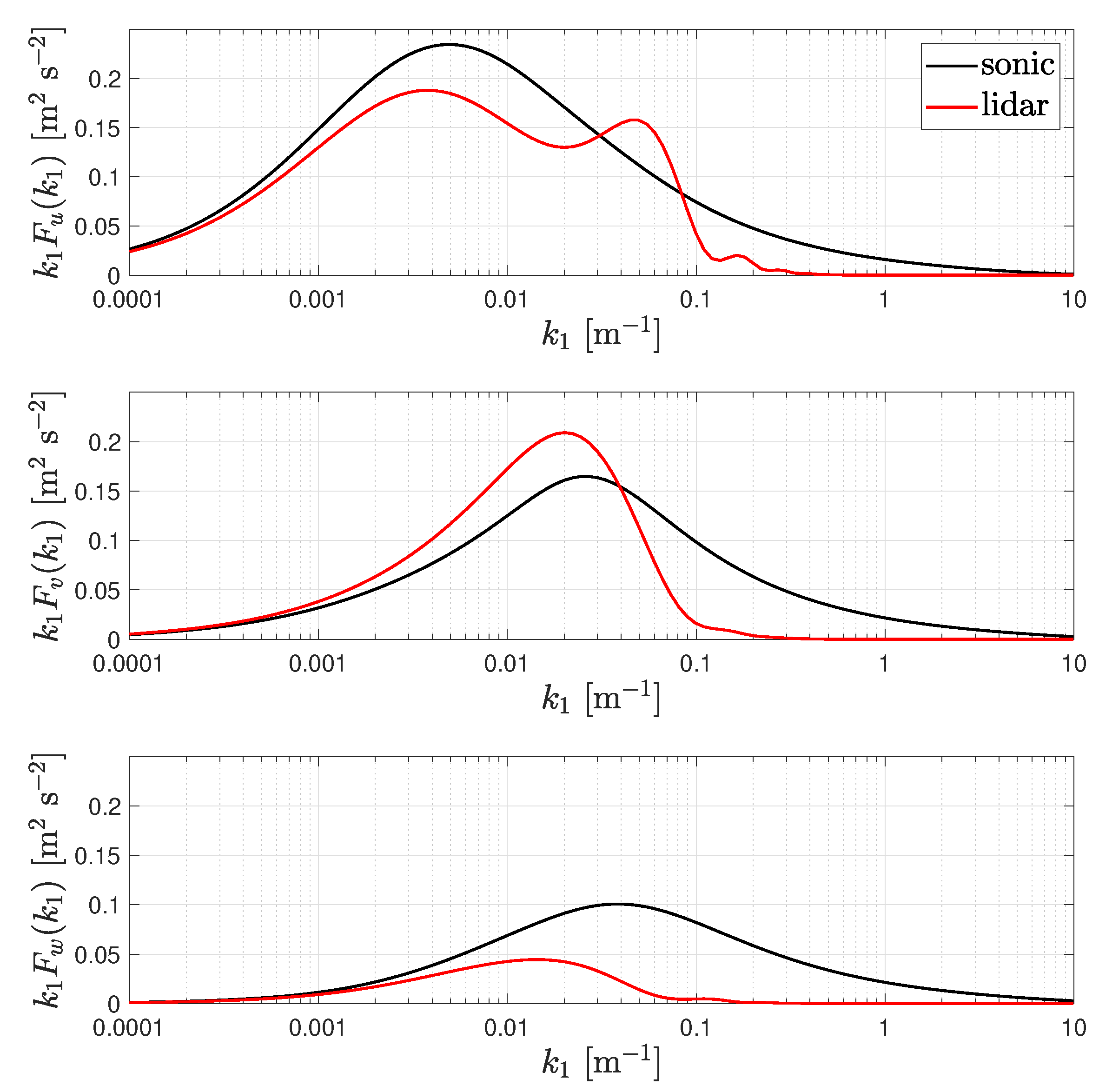
where the subscript i denotes the number of the line-of-sight measurement. Figure 2 shows the velocity spectra of a ZX lidar for a set of Mann parameters assuming m. As illustrated, the spectrum of the three reconstructed velocity components is both ‘contaminated’ by cross-components (easily seen by the multiple peaks) and affected by the averaging effect of the probe volume (decrease in the spectra density with increasing wave number). A way to suppress the contamination was suggested by Kelberlau and Mann [20] and tested on conically scanning lidar data. However, this method requires access to individual line-of-sight velocities.
2.4. Lidar Simulation in a Turbulence Box
Turbulence boxes, i.e., realizations of simulated atmospheric turbulence, which are randomly generated with the Mann model [21], can be used to simulate the measurements performed by lidars. There we can account for the lidars’ scanning configuration, probe volume effects, and buoy’s motion, e.g., for a floating lidar.
We generate 100 random turbulence boxes using different seeds, i.e., different turbulence realizations, but with the same Mann parameters: m s, m, and . With these turbulence characteristics, the target velocity covariances, which one can compute from Equation (11), are m s. As the highest measured level by the lidar investigated here is 100 m (see Section 3), our turbulence boxes have sizes m and number of grid points . This means the resolution of the grid cells is 2 m in all directions. The large size in the x-direction is normally chosen so that the wind flows throughout the box within 10-min or 30-min periods.
The mean velocities of the turbulence boxes are zero and so we can add velocity vertical shear assuming a roughness length mm (close to that of the water surface). For practical purposes, we first estimate the friction velocity for the specified wind speed at a given height h assuming the logarithmic wind profile, thus
where is the von Kármán constant (≈0.4). The vertical profile of mean wind, i.e., , is added to the u-velocity field of the turbulence box. Vertical shear is added as it might have an impact on the estimation of both the mean wind speed and turbulence, as in the simulation we consider that the lidars measure within a probe volume.
2.5. Simulation of the Buoy’s Motion
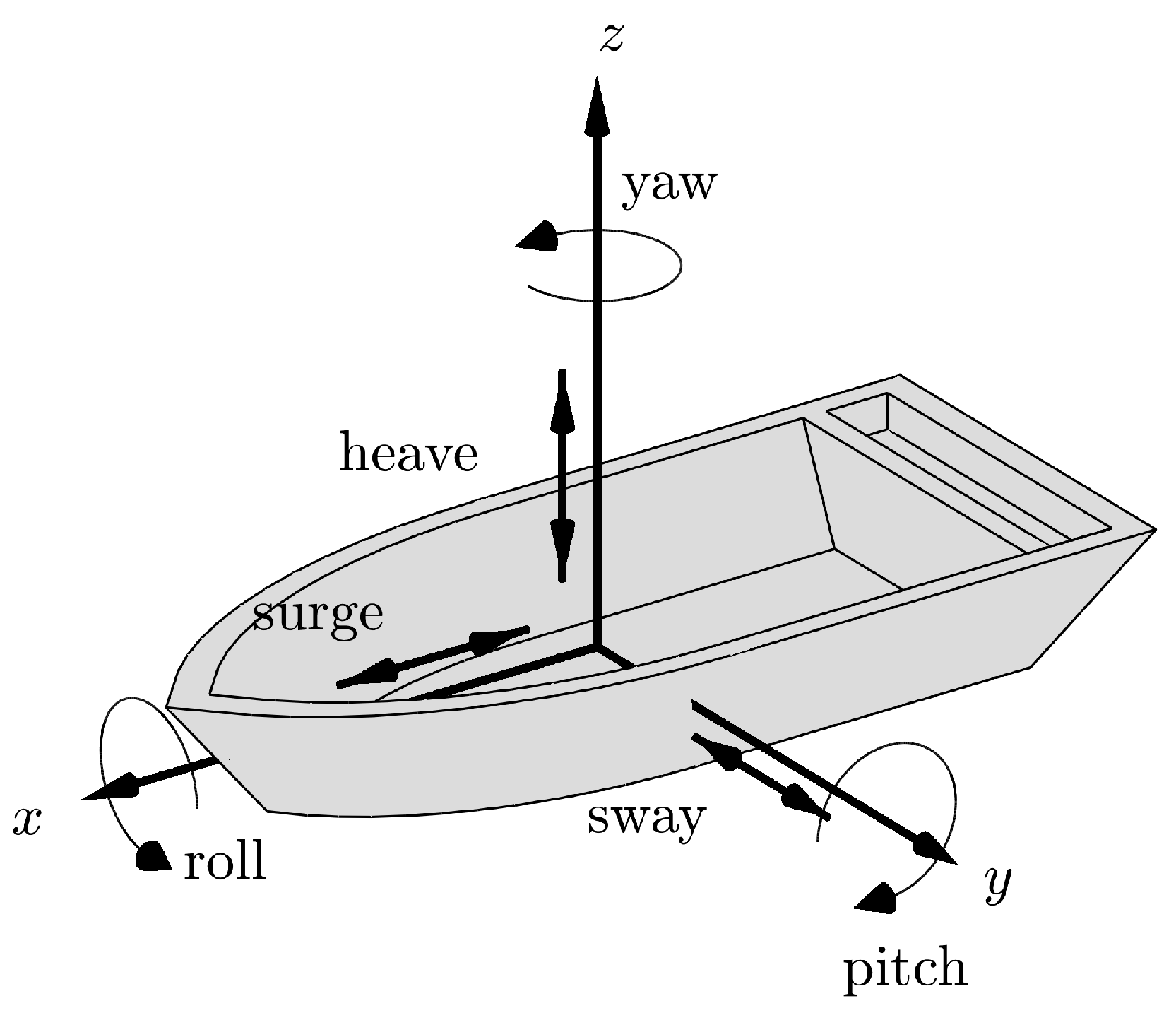
The VAD lidar on a buoy is simulated similarly as the fixed VAD lidar. However, we add the three rotations: pitch, roll and yaw (see Figure 3). On a fixed reference frame, the pitch rotates the buoy around the y-axis,
roll around the x-axis,
and yaw around the z-axis,
The full rotation matrix places the positions of the VAD scan in the new rotated frame of reference:
If the buoy only rotates but does not translate, the radial velocities of the buoy VAD lidar would be expressed as , where is the wind’s velocity vector at the new scanned rotated positions. However, a buoy also translates and so the buoy velocities are added to the wind velocities. The velocities induced by the buoy comprise those in the roll, pitch, and yaw directions, i.e., surge, sway, and heave motions, respectively. If these are measured in the buoy’s frame of reference, we need to transform them with the rotation matrix before adding them to the wind velocities. The new radial velocity that the lidar measures is thus
3. Site, Measurements, and Datasets
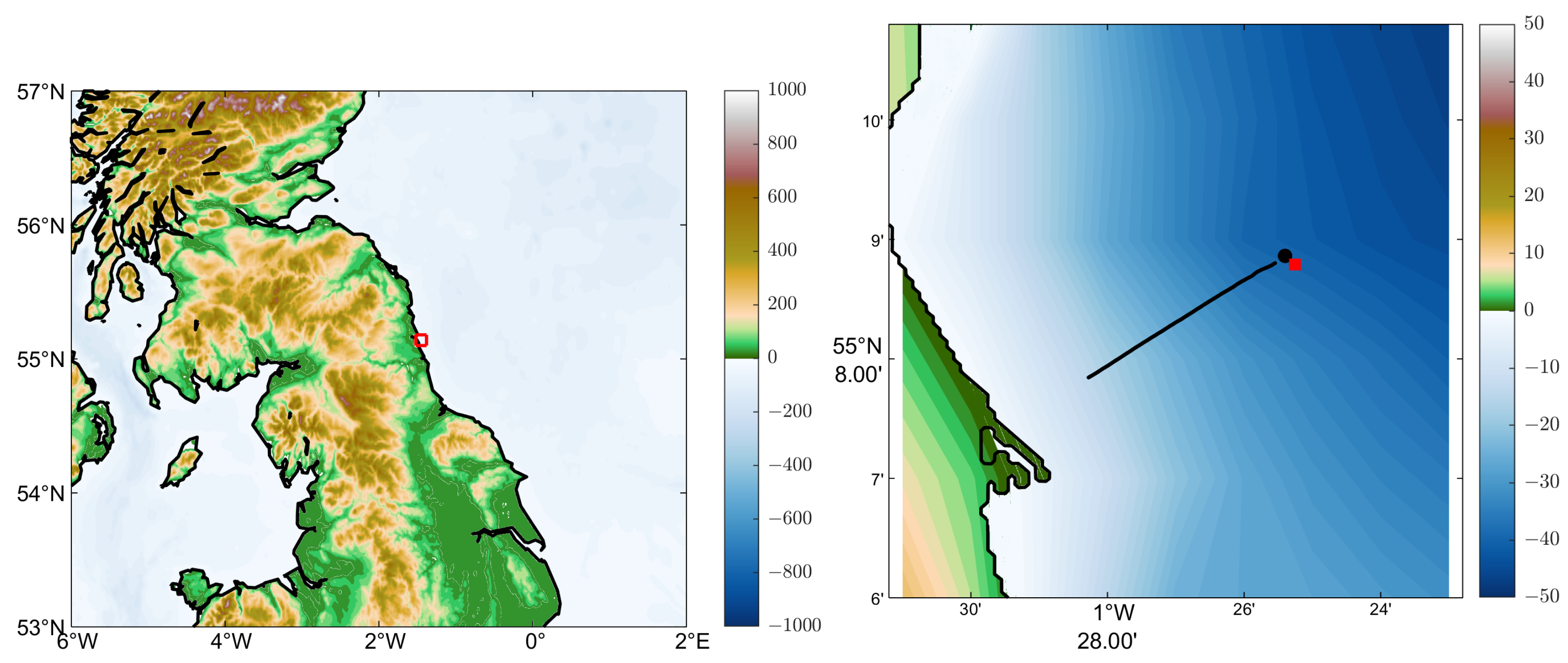
A floating lidar was deployed off the shore near Blyth (UK) from 8 November 2018 to 6 May 2019 (see Figure 4). The Narec offshore anemometry hub (NOAH) meteorological mast is installed about 5.5 km from the coast near Blyth (N, W). The floating lidar GPS recorded the lidar positions, which shows that the buoy was within 126.2 to 3654 m from the mast during the measurement period.
The mast is equipped with cup anemometers at 35, 52, 69, 86, and 103 m above mean sea level (amsl) on the north- and south-facing booms. Vanes are at the same levels except the highest, which is at 101 m amsl. The floating lidar was a ZX300M lidar from ZX lidars on a RPS LiDAR 4.5 Buoy by RPS Australia West, which was equipped with a Kongsberg MRU-5 motion reference unit (MRU) that recorded the motions of the buoy at 2 Hz. The ZX lidar was configured to measure at 11 heights, from which 5 are nearly matching those of the mast (35.3, 52.3, 69.3, 86.3, and 103.3 m amsl). Note that the ZX lidar is on a buoy about 3.3 m amsl.
Most available data (from the ZX lidar, cup anemometers, and buoy) were recorded at 1 Hz. Measurements of the radial velocities are not available from the ZX lidar, as already mentioned, but only the 1-s reconstructed wind speed and direction by the system. As the ZX lidar measured at several heights and needs refocusing, the revisiting time for each height is ≈17 s. Data from the vanes are available as 10-min time series. Buoy data comprise measurements of the pitch, yaw and roll rotations, and heave displacement. We also used the surge, heave, and sway linear velocities, and headings based on a GPS and a magnetic compass.
4. Results
4.1. Simulation Procedure
For both the numerical tests (Section 4.2) and the experimental results (Section 4.3), we use the same procedure to simulate the VAD lidar within the turbulence boxes. The procedure is based on the sequential application of the following operations:
- interpolate motion, rotation, and/or buoy displacements to match the timing of radial velocity measurements by the VAD ZX lidar assuming that the full VAD scan is performed in 1 s. The interpolation is not evenly spaced because the ZX lidar measures at a low frequency (0.06 Hz) due to refocusing;
- simultaneously simulate the ZX lidar for both its fixed and floating configurations by placing them at the bottom of the box at the middle grid point in the y-direction, i.e., . Depending on whether we want to perform a numerical test or simulate the measurements as close as possible (i.e., ≈35 measurements per 10 min), we reconstruct the velocity components by ‘moving’ the lidar either along all grid points in the x-direction or along 35 of the positions covering the length of the box in the x-direction, respectively;
- compute the location of a virtual sonic anemometer on a meteorological mast and of the scans of a fixed lidar without accounting for probe volume;
- for each of the lidar positions in the x-direction, we go through each of the 50 azimuthal positions and apply the interpolated buoy rotations using Equation (22), thus computing the ‘rotated’ unit vector of the floating lidar;
- compute the locations of each of the 50 scanning beams of the floating lidar accounting for the heave displacement (if any). The heave displacement is only added to the vertical component of each location;
- rotate the induced velocities (surge, sway and heave) by the motion of the buoy using the ‘rotated’ unit vector ;
- in parallel account for the probe volume; we determine all the line-of-sight positions within the range for the ZX lidar with a resolution of 0.10 m. We then compute the velocities of these positions using turbulence box velocity interpolants. This is performed for both fixed and floating lidars. For the floating lidar, we also add the induced velocities by the buoy (from the previous step) to the mapped velocities;
- compute for each of the 50 beams, the centroid and median values from the distribution of radial velocities within the probe volume for both the fixed and the floating lidars;
- construct time series of the lidar radial velocities derived from the median and centroid methods. This is performed for both fixed and floating lidars;
- after looping over all 50 azimuthal positions, we map the velocities for both the mast, the fixed and the floating lidars without accounting for probe volume. For the latter, we also include the buoy induced velocities;
- compute the radial velocity of all 50 beams of those 35 positions for the fixed lidar using Equation (4), i.e., the radial velocity is a function of the velocity components, azimuthal orientation, and opening angle;
- construct a time series of lidar-reconstructed velocity components by fitting the previously computed radial velocities to the model used by the ZX lidar, i.e., Equation (5). This is performed for both fixed and floating lidars;
- also construct time series of the lidar-reconstructed velocities derived from the median and centroid methods. This is performed for both fixed and floating lidars;
- compute the means and variances for each of the lidars and methods (centroid and median). We also compute the statistics that a sonic/cup anemometer could output if deployed on a mast, which is virtually ‘moving’ at the same positions of the lidars.
The above procedure is performed sequentially for the amount of vertical levels required (e.g., five for the experimental results). The procedure is then repeated for a number of turbulence boxes (100 for some of the numerical tests and 20 for the experimental results) to reduce the random error of a single turbulence box realization.
4.2. Numerical Tests
4.2.1. Fixed Lidar
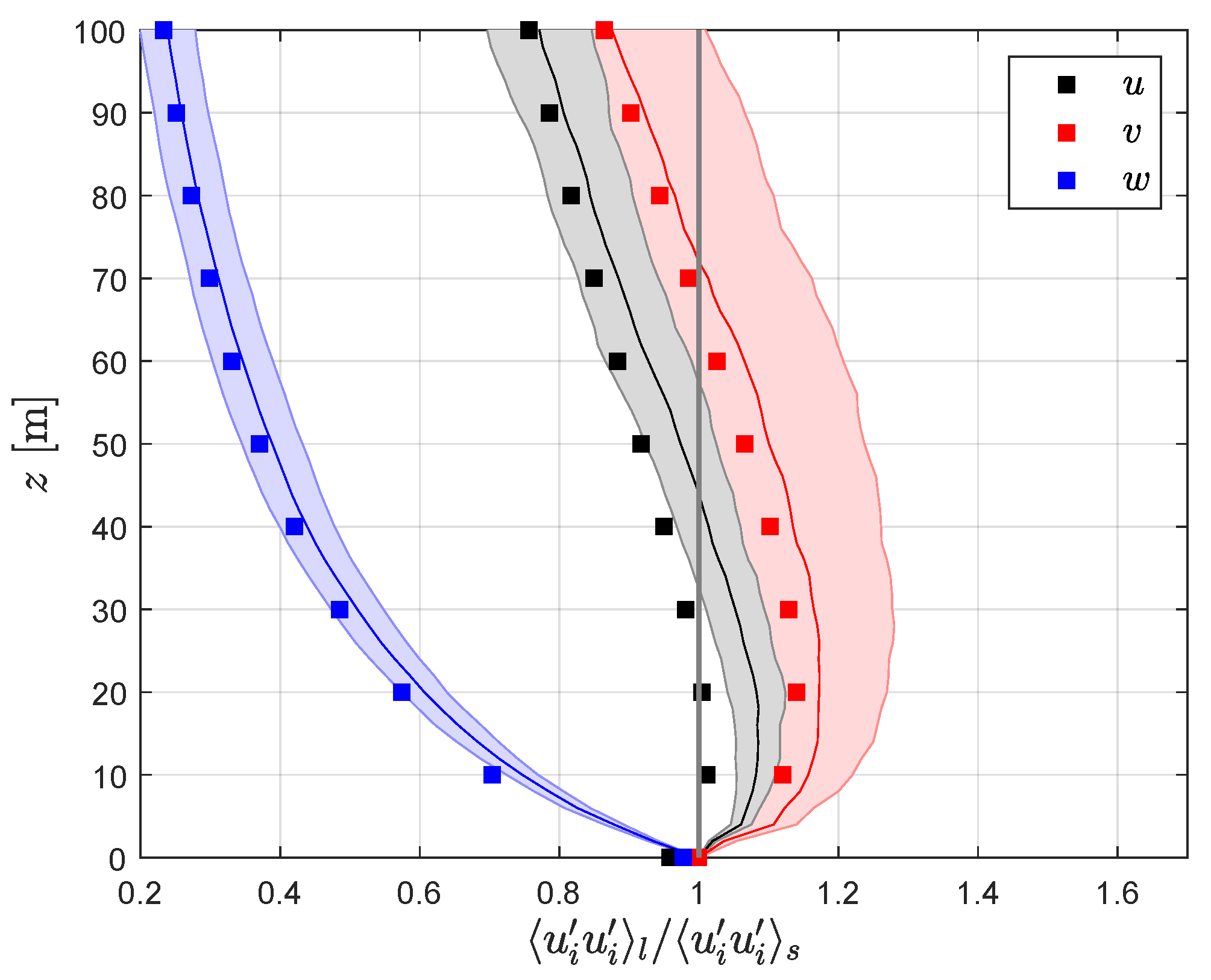
We first simulate the VAD ZX lidar scans within turbulence boxes to test our methods on a fixed lidar. We validate that the velocity variances reconstructed from the VAD lidar simulator follow the theoretical predictions in Section 2.3 using the same Mann parameters as those of the turbulence boxes for all heights. To simplify this validation, we do not account for the lidar probe volume neither when using the turbulence box nor in the theoretical predictions. The comparison between the VAD simulator and the theoretical predictions for the ZX lidar is shown in Figure 5.
As illustrated, the lidar-to-sonic variance ratios computed from the turbulence boxes are very similar to the theoretical predictions. Some differences are due to a bias in the theoretical predictions. At m the variance ratios should be zero for all components. However, at this vertical level, the variance ratio is 0.96 for the u-component and 0.98 for the w-component. The bias in the theoretical predictions is due to the limited azimuthal resolution of the ZX lidar; the higher the number of beams the closer the variance ratios to one.
4.2.2. Floating Lidar
Similarly to the fixed ZX lidar, we simulate the floating lidar’s scanning strategies using the turbulence boxes (for this purpose we use 20 of them only due to computational expenses). The rotation, heave displacement, and translation motions of the buoy are accounted for as cosine waves characterized by an amplitude and a period. With a priori knowledge of the amplitudes and periods of the motions recorded by the buoy close to the NOAH mast, we simulate each of the motions within a fixed range of amplitudes. The amplitudes for linear motions were between 0 and 0.75 m s and for rotations between 0 and 10, except yaw that we limited up to 45. For all these simulations, the period was fixed to 4 s, which is close to the mean period of the surge, sway, and heave linear velocities.
Although not shown, none of the motions simulated has an important impact on the mean reconstructed wind speed by the lidars with or without accounting for the effect of the probe volume. The only motion that impacts significantly the mean wind speed is the yaw; for a cosine wave describing the yaw rotation, the maximum ratio of the floating to the fixed lidar mean wind speed is close to 0.97 for an amplitude of 45. However, this is an extraordinary case as yaw is the motion with the less oscillatory behavior of all. See Kelberlau and Mann [4] for a detailed account for the influence of the buoy motion on the mean wind speed.
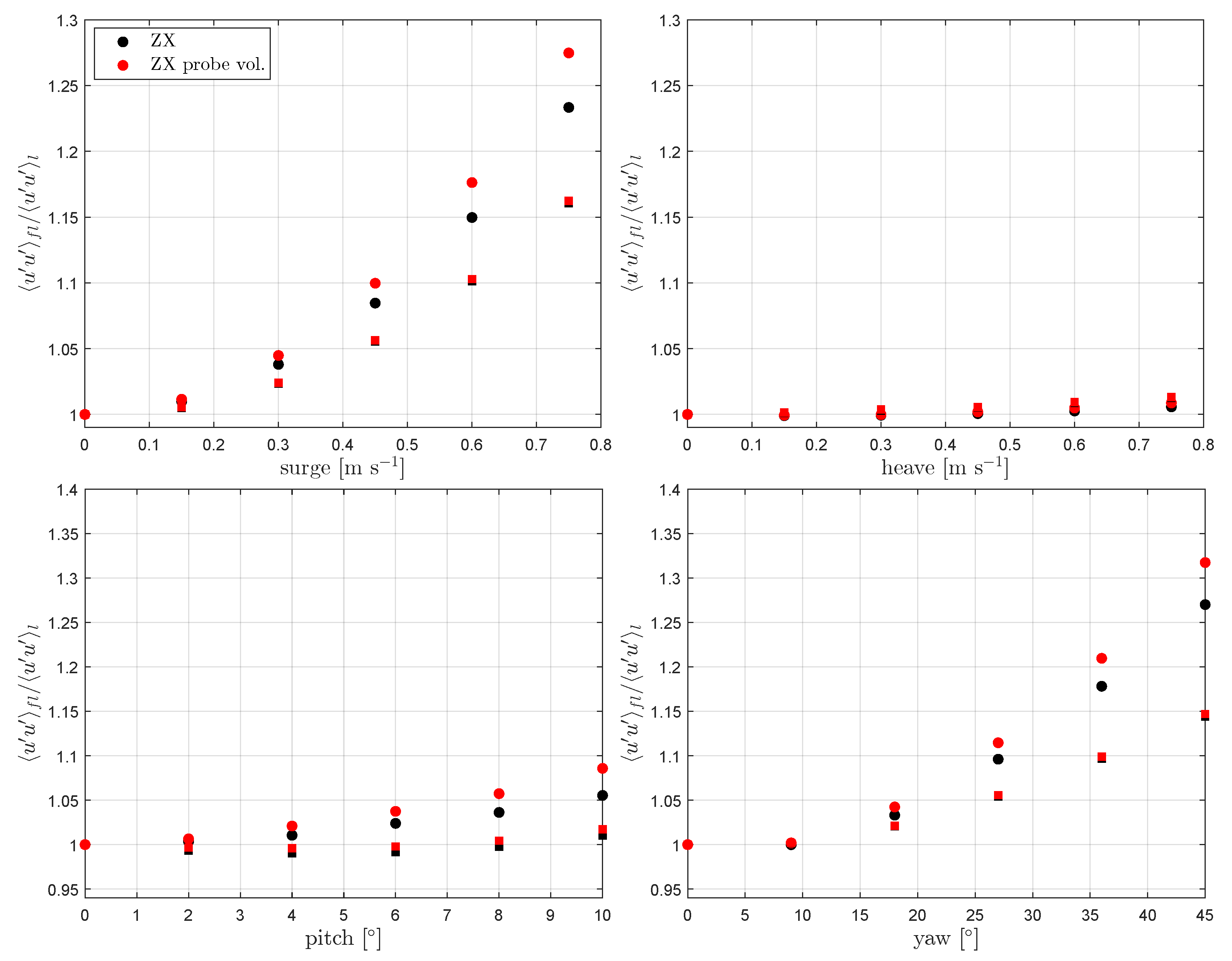
Figure 6, however, shows that the effect of the buoy motions on the ratio of the floating to fixed lidar u-velocity variance can be rather important. Translational motions other than sway (which is nearly perpendicular to the direction of u), in particular surge (Figure 6 top-left frame), can lead to up to ≈30% more variance measured by a floating compared to a fixed ZX lidar. When looking at the surge motion, the effect of the increasing probe volume of the ZX lidar is clearly observed as this is largest at the highest simulated height (100 m). The effect of heave motion is not as high as that of surge; it is below 2%. The influence of sway is quite low (not shown). For the pitch rotation, in particular, we find up to a 10% increase in the u-velocity variance for the ZX lidar when measuring at 100 m. We also show the variance ratios for yaw amplitudes of 45 to find out whether these could be as high as those resulting from pitching the buoy. As illustrated, for the ZX lidar, the effect of the yaw rotation is always to increase the variance; at 100 m it is close to 30% higher than the fixed value.
4.3. Experimental Results
4.3.1. Filtering Procedures
We compute 10-min statistics (means and variances) of the reconstructed horizontal wind speed of the ZX lidar and the cup anemometers for the whole period. Within the extent of the measurement campaign, there are potentially 25,920 10-min periods for analysis. However, in 2233 of those periods, data from either of the instruments are missing. For the comparison of the 10-min statistics, we also apply the following filtering scheme (in parenthesis the number of 10-min intervals that the specific criterion eliminates):
- Lidar reconstructed horizontal mean wind speeds should be lower than 99 m s (4801)
- Lidar, at the heights where the ZX lidar measures close to the cups, and cup anemometer 10-min time series should include more than 32 and 590 records, respectively (1401)
- Cup anemometers should all measure simultaneously winds with speeds larger than 1 m s (1019)
- The buoy, where the lidar was deployed, and the NOAH meteorological mast should be closer than 1 km (2840)
After filtering, 14,925 10-min periods are left for analysis. Since we have two cup anemometers at each height, we choose the one giving the highest wind speed as an attempt to reduce the influence of mast shadowing. Further, the ZX lidars usually record a measure of the signal’s backscatter (sometimes referred to as the spectra scaling ratio), which can be used to filter for, e.g., contamination of the Doppler spectra due to clouds [22]. Such contamination impacts the radial velocities measured at the high focused heights mostly (so the reconstructed wind speeds are positively biased), since at these heights the measurement volume increases considerably. Unfortunately, these records are not available from this campaign. By a preliminary comparison (not shown) between the cups and the lidar mean wind speeds at the lowest and highest heights, we observe these positive biases. A number of 10-min periods show a much higher mean wind speed observed by the ZX lidar compared to that of the cup anemometer at the highest level, while the two instruments show mean values that are very close at the low heights. We speculate that these outliers are mainly due to cloud contamination and we filter them by selecting 10-min periods, where the lidar-based wind speed ratio between the highest and lowest height is within the cup-based one. After applying this last filter, 13,419 10-min periods are finally left for analysis. Filtering for rain (based on the sensor on the ZX lidar) does not improve the wind speed comparisons between the ZX lidar and the cup anemometers; it mainly decreases the amount of data.
4.3.2. Statistics without Motion Compensation
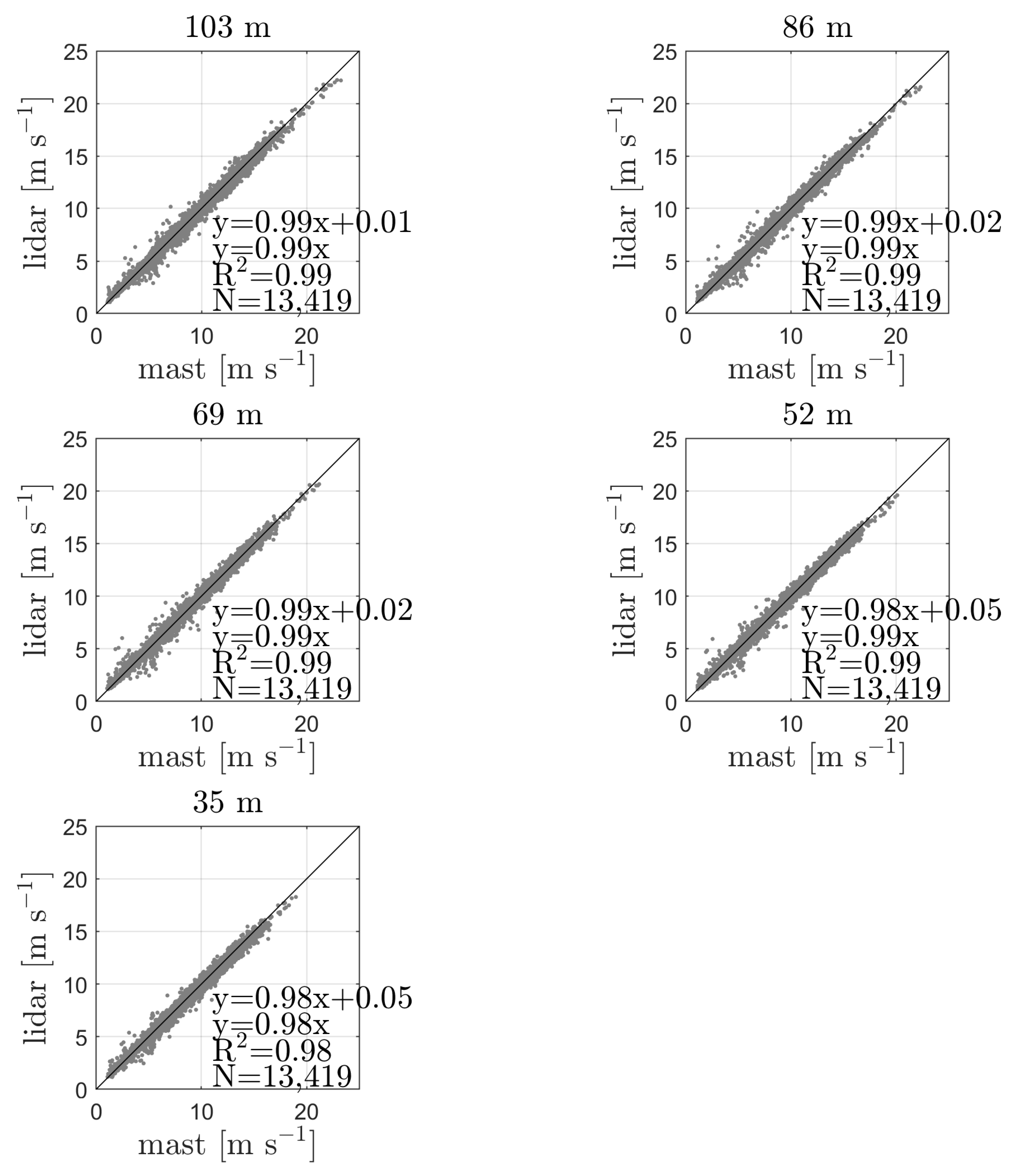
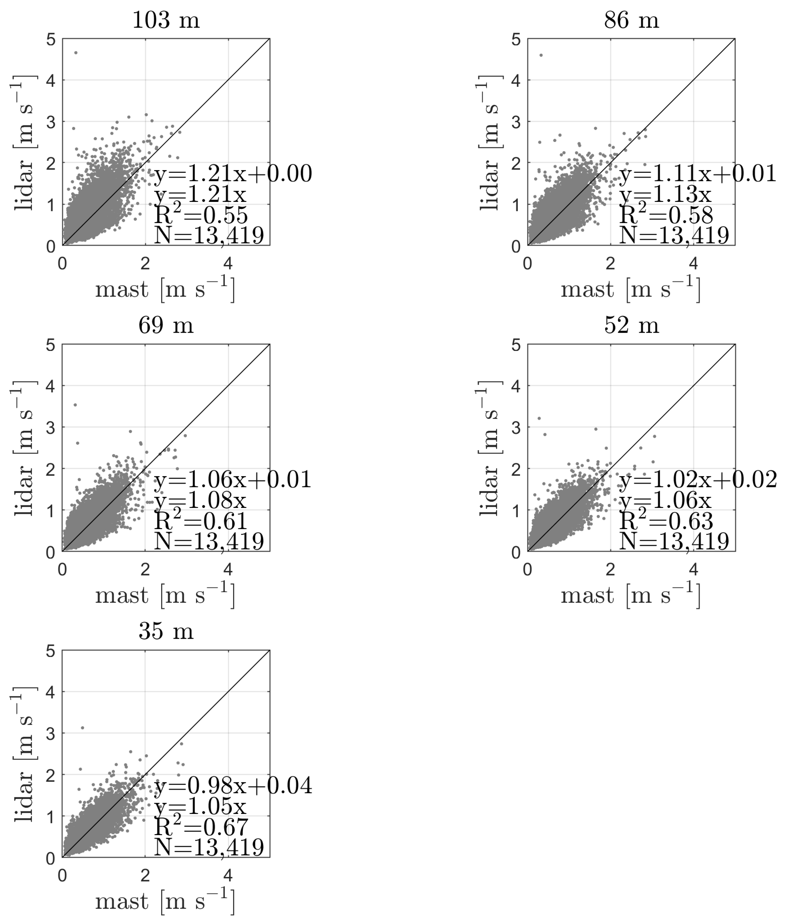
Figure 7 shows the comparison between the 10-min means of the ZX lidar reconstructed horizontal wind speeds and those of the cup anemometer at the closest height. As illustrated and expected, the agreement is rather good with the largest bias of ≈2% at the lowest level, where we also find the lowest coefficient of determination R. Although not shown, note that if we include the ≈1500 10-min periods in which the wind speed ratio measured by the ZX lidar is beyond of that measured by the cup anemometers, we find most of these periods above the 1:1 relation in Figure 7. These periods become also more scattered the higher the observed height, thus decreasing slightly the correlation with height.
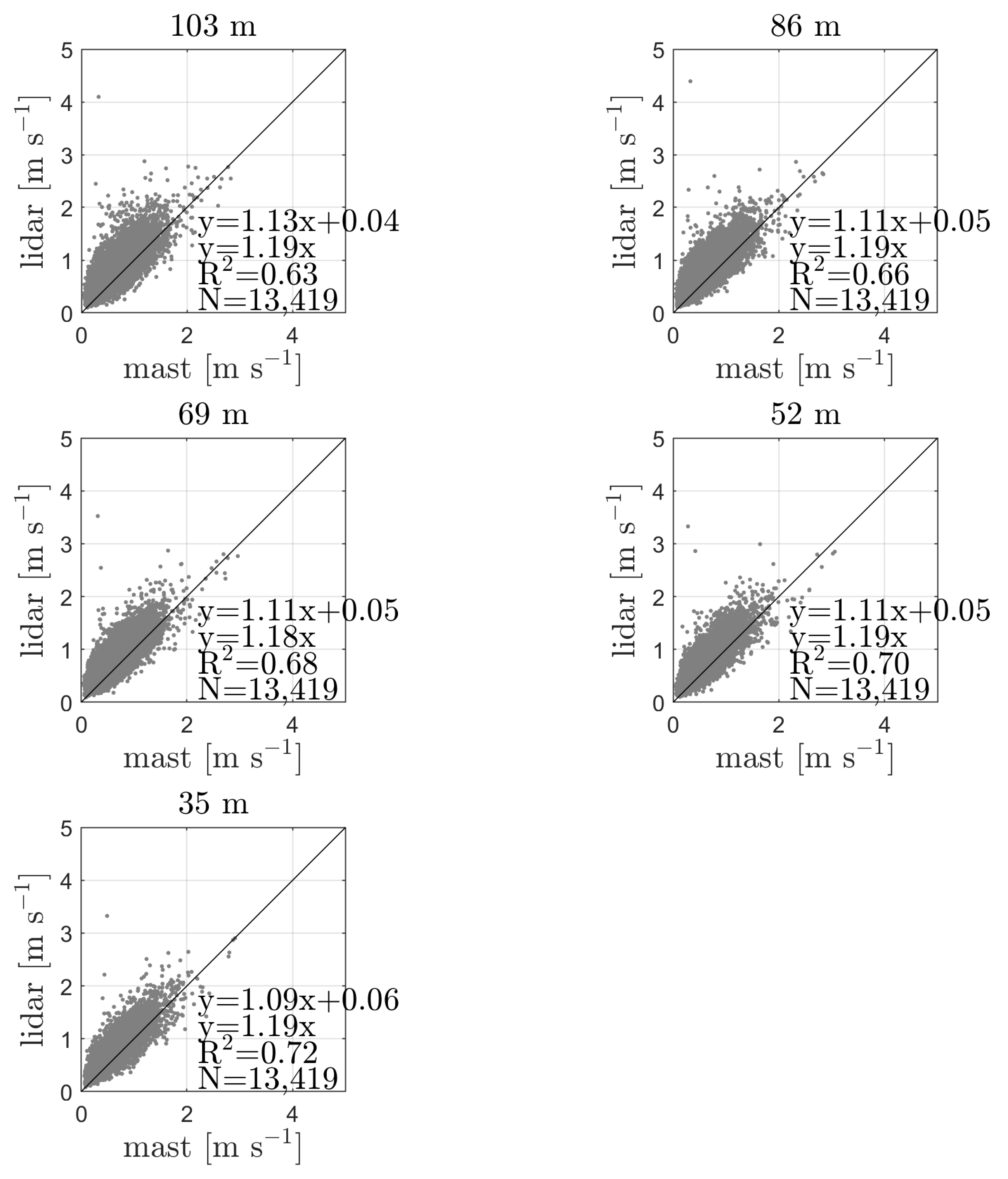
We also show the comparison of turbulence estimates, in this case of the standard deviation of the 10-min reconstructed horizontal wind speeds between the ZX lidar and the closest cup anemometer (see Figure 8). As illustrated, turbulence measured by the ZX lidar is generally larger than that of the cup anemometer at all heights. The bias between the measurements is within 18–19% at all levels. The correlations are not as high as those of the mean wind speeds in Figure 7 and they decrease slightly with increasing height.
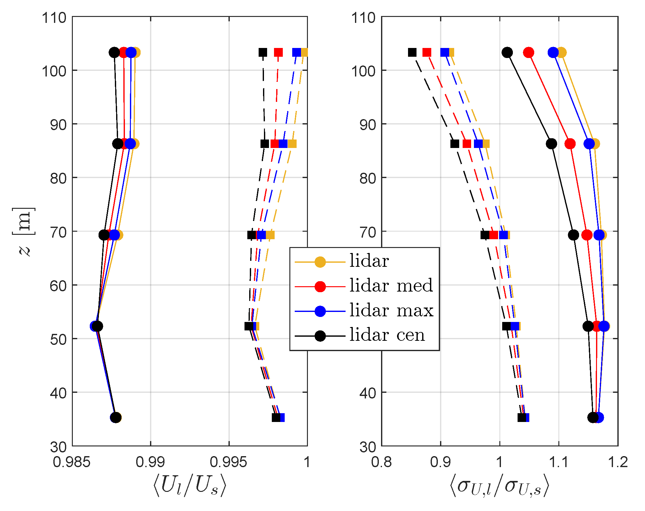
The output of the simulation procedure in Section 4.1, when applied to the buoy measurements within the 13,419 10-min periods of the campaign, consists of a series of mean and standard deviation computations for each 10-min period. This output includes results for each of the 20 turbulence boxes as well as those of the simulated cup anemometer and lidar measurements, which also cover the different methods accounting (or not) for the probe volume. Figure 9 illustrates the overall results of the motion correction when assuming that at a yaw of 0 the lidar coordinate system matches the azimuthal position of 0 and that this azimuthal position is always oriented with the wind direction. The figure shows the ensemble average (over all 10-min periods and 20 turbulence boxes) of the ratios of the ZX lidar computation (either buoy or fixed and with or without probe volume) to those of the cup anemometer computation of both the mean and the standard deviation of the horizontal wind for the five measurement heights.
As illustrated, the effect of the buoy rotation/translation on the mean horizontal velocity estimated by the ZX lidar is very small with or without probe volume. For all cases (probe-volume wise) and all vertical levels, the mean horizontal wind speed is underestimated by the floating ZX lidar between 1.25–1.0%, which is in close agreement with the results of the measurements regarding the mean wind speeds (Figure 7). For the fixed lidar, we see the same pattern but much lower biases (0–0.5%). Kelberlau and Mann [4] quantified the relative error on the mean wind due to the motion of a floating lidar. For motion frequencies close to 0.3 Hz (which is close to the mean motion frequency of the buoy close to NOAH), they found nearly no error on the mean wind due to pitch and slightly negative values (close to −0.005) due to yaw. Their findings are consistent with our results where the floating lidar to cup ratios are between 0.985 and 0.99 for the mean wind.
However, as expected, the effect of the buoy rotation/translational motion on the standard deviation of the horizontal velocity measured by the ZX lidar is large. In all cases (with or without probe volume) and all vertical levels examined, the floating ZX lidar measures (in average) more fluctuations, and thus, larger standard deviations of the horizontal velocity compared to those of the cup anemometers at the same height. This is in agreement with the analysis of measurements in Figure 8. The largest ratio is found at 52 m; for the no probe volume case (solid yellow line), the floating lidar standard deviation is 17.8% larger than that of the cup anemometer. When accounting for the probe volume and using the median estimate (solid red line), the figure reduces to 16.4% for the same height. At 103 m, we find the lowest ratios; for the no probe volume case, the floating ZX lidar standard deviation is 10.4% larger than that of the cup anemometer, whereas the value reduces to only 1.3% for the centroid estimate. It can also be observed that when accounting for probe volume we see a systematic reduction of the ratios. From largest to lowest reduction compared to the no-probe volume case we have the centroid, the median, and maximum estimates, as expected. The results for the maximum estimate appear nearly on top of those of the no probe volume case, both for the floating and fixed ZX lidar. For the fixed ZX lidar, we notice a reduction on the turbulence measures when compared to the cup anemometer from 69 m upwards. Note that these results are the ensemble averages for all the 13,419 10-min periods in which we have complete time series of buoy rotations and translations.
4.3.3. Statistics with Motion Compensation
We compute the motion-compensated estimates of the horizontal velocity mean and standard deviation using the compensation factors that we compute for each 10-min period of the measuring campaign. The compensation factors are equal to the ZX lidar to cup anemometer ratios of the mean and standard deviation of the horizontal velocity, which we derive from the procedure delineated in Section 4.1. Note that the ensemble averages of these ratios are shown in Figure 9. Figure 10 illustrates results of this compensation for the standard deviation of the reconstructed horizontal velocity of the floating ZX lidar. Compared to the results without compensation (Figure 8), the mean biases are reduced to 5%, 6%, 8% and 13% for Deming regressions (1%, 2%, 3%, and 7% for linear regressions, which are not shown) for the heights 35, 52, 69, and 86 m, respectively. These reductions are expected, since the average lidar to cup standard deviation of horizontal velocity ratio is between 10–20% within these vertical levels (see Figure 9). However, the mean bias at 103 m does not change much when compared to the results without compensation. At this height, the simulations using the median method show that this bias should be around 4.9% on average for the floating ZX lidar (Figure 9). Clearly, the simulated effect of the buoy’s motion does not help to reduce the turbulence overestimation at this height. We notice (not shown) that at 35 m, simulated ZX lidar to cup anemometer wind speed standard deviation ratios are all above unity. When increasing the height, these ratios can appear below unity within the entire range of observed turbulence levels. At 103 m, 10-min periods with ratios below unity dominate over those above unity when the cup anemometer wind speed standard deviation is larger than 1.5 m s. This effect can be observed when comparing the scatter plots at 103 m between Figure 8 and Figure 10.
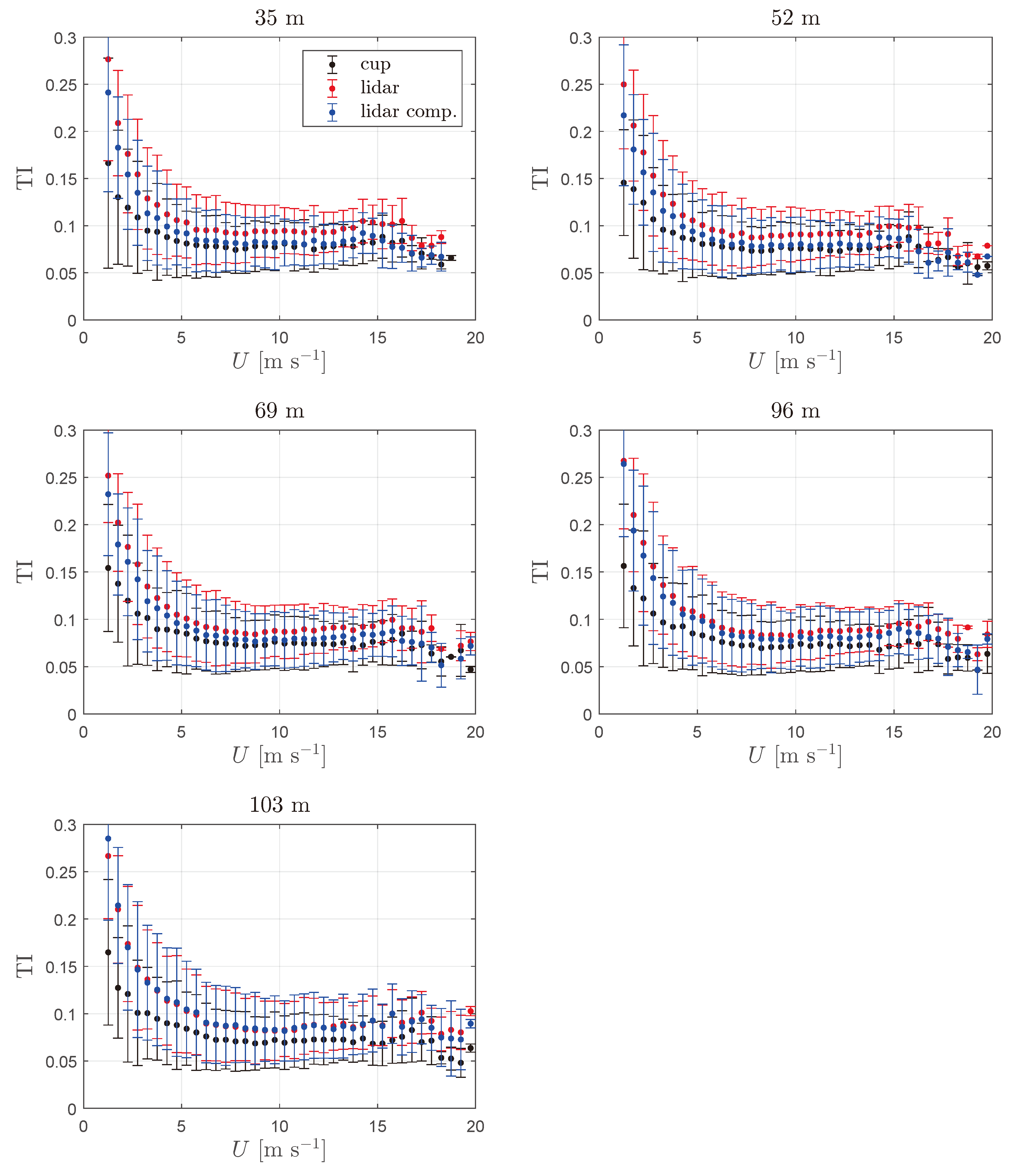
We also present the results of the ‘turbulence’ compensation by illustrating the TI computed at several horizontal wind speed bins for each of the measured heights (Figure 11). At 35 m, the floating ZX lidar compensated TI is lower than the floating ZX lidar original TI for all velocity bins. One can notice that the floating ZX lidar compensated TI becomes closer to the cup-based value within the wind speed range 5–15 m s when compared to the wind speed range 1–5 m s. The difference between the cup and floating ZX lidar (compensated or not) TI estimates tends to increase the lower the wind speed, where the TI estimates based on all instruments also increase. The increase in TI within the low speed range is generally due to the influence of atmospheric stability as stable and unstable conditions concentrate within this wind speed range. This influence diminishes with increasing wind speed as neutral atmospheric conditions become dominant under high wind conditions. Assuming the logarithmic wind profile (Equation (18)) and that , . Thus, assuming mm, TI is between 0.083 and 0.076 within the measurement levels (35–103 m), which are close to the values that TI asymptotically reaches beyond m s in Figure 11. Within the wind speed range 1–5 m s, probe volume and cross-contamination effects can be different than those estimated with the turbulence boxes used to estimate the turbulence errors. This is because both the anisotropy and length scale that one could obtain from the measurements within this speed range might be different to those used for generating the Mann model turbulence boxes in which the floating lidar is simulated ( and m).
For the heights between 52–96 m, we see similar results when compared to those at 35 m. However, as expected from the mean biases observed in Figure 10, the floating ZX lidar-compensated TI values approach the cup-based TI values less closely with increasing height. At 103 m, on the other hand, the floating ZX lidar-compensated values are nearly on top of those without compensation, which explains the low change in mean bias between the results with and without compensation at this height.
5. Discussion
Our procedure to simulate the error on floating lidar measurements due to the motion of the buoy relies on the use of time series of buoy motions within each 10-min period where there are buoy records. With this information, we are able to estimate the ratio of the lidar to cup anemometer error in both the mean and variance of the reconstructed horizontal wind speed. The procedure is based on the simulation of the VAD scanning configuration of the lidar within atmospheric turbulence boxes. Based on these simulations, we find that on average a floating lidar overestimates the standard deviation of the horizontal wind speed when compared to the estimate by a cup anemometer measuring at the same vertical level. The overestimation decreases when the probe volume is taken into account and depends on the method used to estimate the ‘weighted’ radial velocity estimate. For reference, a fixed lidar also overestimates turbulence measures but only within the closest heights to the surface due to cross-contamination of the velocity components.
It is important to note that when we simulate the buoy motions for each 10-min period within the turbulence boxes, we do not account for differences between the wind direction and the heading of the buoy. As the ZX lidar measures at 50 azimuthal positions, the influence of any misalignment should be negligible. Future studies could try to analyze whether using the headings and compass signals of both the ZX lidar and the buoy improves the error estimations.
A possible improvement of the method is the use of different turbulence boxes for the different turbulence conditions that the atmospheric can experience with time and height. As shown from the results of the TI variation with wind speed, the method works best under high wind speed conditions. However, the differences between the cup anemometer and floating ZX lidar TIs are largest at lower wind speeds. Here, for simplicity and computational expenses, all turbulence boxes are generated using the same Mann parameters. However, we are aware that these parameters depend, among others, on atmospheric stability (and thus turbulence itself) and height [18].
6. Conclusions
From both cup anemometer measurements on the NOAH meteorological mast and ZX lidar measurements on a buoy nearby, we find a nearly zero mean bias when comparing the 10-min mean wind speeds at the heights where both systems measure the closest (35, 52, 69, 86, and 103 m). When comparing the 10-min standard deviation of the reconstructed horizontal wind speed between the two systems, we find that the floating ZX lidar measures about 18–19% more turbulence intensity than the cup anemometers. These mean biases are computed after a number of 10-min periods are removed from the analysis, as cloud or noise contamination might be present. Such contamination becomes more evident at the highest observation heights.
We correct the lidar measurements of turbulence for buoy motion induced errors by simulating the lidar measurements within synthetic fields of atmospheric turbulence. After correction, we compare these lidar measurements of turbulence with those from the cup anemometers. We find lower mean biases for the first four vertical levels (5–14%). For the highest vertical level (103 m), the mean bias (19%) does not change after error compensation, although the simulations show a possible mean bias correction of ≈4%. This could be due to the use of homogeneous turbulence boxes in our simulations. Although all boxes are generated randomly and are independent realizations of turbulence, their turbulence characteristics do not change with height. As shown in Pena [18], turbulence characteristics and thus the Mann parameters change with height.
When looking at the turbulence intensity variation with wind speed for the four lowest levels, we observe that the compensated estimates of the floating ZX lidar are much closer to the cup anemometer estimates than the case without error compensation. This occurs for a wide range of wind speeds (1–20 m s). The agreement is stronger the larger the wind speed and the closer the level is to the surface. At the highest level, whether error compensated or not, the turbulence intensity by the lidar is higher than that of the cup anemometer.
Author Contributions
A.P. performed the analysis of the measurements, produced the results and figures, and drafted the manuscript. A.P., J.M. and N.A. conceptualized and designed the analysis. A.P. and J.M. developed the methodology. A.J. provided the resources and materials. All authors contributed with the manuscript review and edition. N.A. and A.J. executed the funding acquisition. All authors read and agreed to the published version of the manuscript.
Funding
The study was financed by Equinor ASA, contract number 4590237363.
Data Availability Statement
The measurements are property of Equinor and they should be contacted for getting access. The codes to reproduce all numerical results, as well as the turbulence boxes can be requested to A.P.
Acknowledgments
We thank RPS Australia West for their continuous support during this work. We also thank the four reviewers for the valuable comments and suggestions.
Conflicts of Interest
The authors declare no conflict of interest.
References
- Gottschall, J.; Gribben, B.; Stein, D.; Würth, I. Floating lidar as an advanced offshore wind speed measurement technique: Current technology status and gap analysis in regard to full maturity. WIREs Energy Environ. 2017, 6, e250. [Google Scholar] [CrossRef]
- Gottschall, J.; Wolken-Möhlmann, G.; Viergutz, T.; Lange, B. Results and Conclusions of a Floating-lidar Offshore Test. Energy Procedia 2014, 53, 156–161. [Google Scholar] [CrossRef]
- Mathisen, J.P. Measurement of wind profile with a buoy mounted lidar. Energy Procedia 2013, 12, 145. [Google Scholar]
- Kelberlau, F.; Mann, J. Quantification of Motion-Induced Measurement Error on Floating Lidar Systems. Atmos. Meas. Technol. Discuss. 2022, 15, 5323–5341. [Google Scholar] [CrossRef]
- Kelberlau, F.; Neshaug, V.; Lønseth, L.; Bracchi, T.; Mann, J. Taking the Motion out of Floating Lidar: Turbulence Intensity Estimates with a Continuous-Wave Wind Lidar. Remote Sens. 2020, 12, 898. [Google Scholar] [CrossRef] [Green Version]
- Tiana-Alsina, J.; Gutiérrez, M.A.; Würth, I.; Puigdefábregas, J.; Rocadenbosch, F. Motion compensation study for a floating Doppler wind LiDAR. In Proceedings of the 2015 IEEE International Geoscience and Remote Sensing Symposium (IGARSS), Milan, Italy, 26–31 July 2015; pp. 5379–5382. [Google Scholar]
- Gutiérrez, M.A.; Tiana-Alsina, J.; Bischoff, O.; Cateura, J.; Rocadenbosch, F. Performance evaluation of a floating Doppler wind lidar buoy in mediterranean near-shore conditions. In Proceedings of the 2015 IEEE International Geoscience and Remote Sensing Symposium (IGARSS), Milan, Italy, 26–31 July 2015; pp. 2147–2150. [Google Scholar]
- Gutiérrez-Antuñano, M.A.; Tiana-Alsina, J.; Salcedo, A.; Rocadenbosch, F. Estimation of the Motion-Induced Horizontal-Wind-Speed Standard Deviation in an Offshore Doppler Lidar. Remote Sens. 2018, 10, 2037. [Google Scholar] [CrossRef] [Green Version]
- Yamaguchi, A.; Ishihara, T. A new motion compensation algorithm of floating lidar system for the assessment of turbulence intensity. J. Phys. Conf. Series 2016, 753, 072034. [Google Scholar] [CrossRef]
- Held, D.P.; Mann, J. Comparison of methods to derive radial wind speed from a continuous-wave coherent lidar Doppler spectrum. Atmos. Meas. Technol. 2018, 11, 6339–6350. [Google Scholar] [CrossRef] [Green Version]
- Sonnenschein, C.M.; Horrigan, F.A. Signal-to-noise relationships for coaxial systems that heterodyne backscatter from the atmosphere. Appl. Opt. 1971, 10, 1600–1604. [Google Scholar] [CrossRef] [PubMed]
- Angelou, N.; Mann, J.; Sjöholm, M.; Courtney, M. Direct measurement of the spectral transfer function of a laser based anemometer. Rev. Sci. Instrum. 2012, 83, 033111. [Google Scholar] [CrossRef] [PubMed] [Green Version]
- Mann, J. The spatial structure of neutral atmospheric surface-layer turbulence. J. Fluid Mech. 1994, 273, 141–168. [Google Scholar] [CrossRef]
- Peña, A.; Gryning, S.E.; Mann, J. On the length-scale of the wind profile. Q. J. Royal Meteorol. Soc. 2010, 136, 2119–2131. [Google Scholar] [CrossRef]
- Sathe, A.; Mann, J.; Barlas, T.; Bierbooms, W.A.A.M.; van Bussel, G.J.W. Influence of atmospheric stability on wind turbine loads. Wind Energy 2013, 16, 1013–1032. [Google Scholar] [CrossRef]
- Kelly, M. From standard measurements to spectral characterization: Turbulence length scale and distribution. Wind Energy Sci. 2018, 3, 533–543. [Google Scholar] [CrossRef] [Green Version]
- Cheynet, E.; Jakobsen, J.B.; Reuder, J. Velocity spectra and coherence estimates in the marine atmospheric boundary layer. Bound.-Layer Meteorol. 2018, 169, 429–460. [Google Scholar] [CrossRef]
- Peña, A. Østerild: A natural laboratory for atmospheric turbulence. J. Renew. Sustain. Energ. 2019, 11, 063302. [Google Scholar] [CrossRef] [Green Version]
- Sathe, A.; Mann, J.; Gottschall, J.; Courtney, M.S. Can wind lidars measure turbulence? J. Atmos. Ocean. Technol. 2011, 28, 853–868. [Google Scholar] [CrossRef] [Green Version]
- Kelberlau, F.; Mann, J. Better turbulence spectra from velocity–azimuth display scanning wind lidar. Atmos. Meas. Technol. 2019, 12, 1871–1888. [Google Scholar] [CrossRef] [Green Version]
- Mann, J. Wind field simulation. Prob. Engng. Mech. 1998, 13, 269–282. [Google Scholar] [CrossRef]
- Peña, A.; Hasager, C.B.; Gryning, S.E.; Courtney, M.; Antoniou, I.; Mikkelsen, T. Offshore wind profiling using light detection and ranging measurements. Wind Energ. 2009, 12, 105–124. [Google Scholar] [CrossRef]
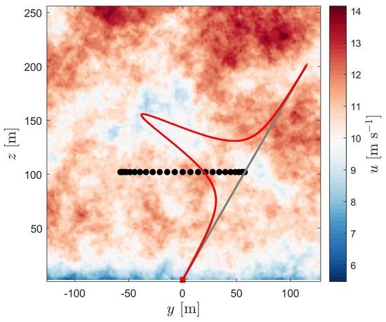
Figure 1.
A typical VAD configuration, where the lidar scans at 50 azimuthal positions.

Figure 2.
Velocity spectra (u-top, v-middle, and w-bottom) for an ideal sonic anemometer and a ZX lidar measuring at a height of 50 m with m s, m, and .
Figure 2.
Velocity spectra (u-top, v-middle, and w-bottom) for an ideal sonic anemometer and a ZX lidar measuring at a height of 50 m with m s, m, and .

Figure 3.
An illustrative sketch of the rotational and translational motions on a floating platform.
Figure 3.
An illustrative sketch of the rotational and translational motions on a floating platform.

Figure 4.
(left) The study area near Blyth (UK) in the red rectangle. (right) The position of the NOAH meteorological mast (red square), the initial position of the floating lidar (black circle) and the positions recorded by the lidar GPS (black dots) during the measurement period. The colorbar indicates the elevation of the terrain in meters relative to the mean sea level.

Figure 5.
Ratio of the u-, v-, and w-velocity variances measured by a VAD ZX lidar (subscript l) to that measured by an ideal sonic anemometer (subscript s) as function of height. Markers correspond to theoretical predictions, and lines and shaded areas are the mean and standard deviation, respectively, of 100 turbulence boxes.

Figure 6.
Ratio of the u-velocity (along-wind) variance measured by a VAD floating ZX lidar (subscript ) to that measured by a VAD fixed ZX lidar (subscript l) as function of the amplitude of the motion (surge in top-left, heave in top-right, pitch in bottom-left, and yaw in bottom-right frame). Results with and without probe volume are shown (see legend). Square and circle markers correspond to a height of 30 and 100 m, respectively. Results correspond to the means of 20 turbulence boxes. The period of the motion is 4 s.

Figure 7.
Scatter plots of the mean wind speed by the cup anemometers on the meteorological mast and the ZX lidar at different heights. The solid black line corresponds to a 1:1 relation. Deming regressions (with and without intercept) as well as the coefficient of determination R and the number of samples N are also given for each height.

Figure 8.
Similar to Figure 7 but for the standard deviation of the wind speed.
Figure 8.
Similar to Figure 7 but for the standard deviation of the wind speed.

Figure 9.
ZX lidar to cup anemometer ratio averaged over all 10-min periods and 20 turbulence boxes of the mean (left) and standard deviation (right) of the horizontal velocity. The solid and dashed lines correspond to the floating and fixed lidars, respectively. The results ‘lidar’ (in the legend) correspond to those without accounting for the probe volume.

Figure 10.
Similar to Figure 8 but for the compensated standard deviation of the horizontal wind speed from the ZX lidar.
Figure 10.
Similar to Figure 8 but for the compensated standard deviation of the horizontal wind speed from the ZX lidar.

Figure 11.
Turbulence intensity (TI) over a number of horizontal velocity bins computed from the cup anemometer, the ZX lidar, and the ZX lidar turbulence compensated measurements for each of the observed vertical levels. Error bars denote ±one standard deviation.
Figure 11.
Turbulence intensity (TI) over a number of horizontal velocity bins computed from the cup anemometer, the ZX lidar, and the ZX lidar turbulence compensated measurements for each of the observed vertical levels. Error bars denote ±one standard deviation.

Publisher’s Note: MDPI stays neutral with regard to jurisdictional claims in published maps and institutional affiliations. |
© 2022 by the authors. Licensee MDPI, Basel, Switzerland. This article is an open access article distributed under the terms and conditions of the Creative Commons Attribution (CC BY) license (https://creativecommons.org/licenses/by/4.0/).
Share and Cite
MDPI and ACS Style
Peña, A.; Mann, J.; Angelou, N.; Jacobsen, A. A Motion-Correction Method for Turbulence Estimates from Floating Lidars. Remote Sens. 2022, 14, 6065. https://doi.org/10.3390/rs14236065
AMA Style
Peña A, Mann J, Angelou N, Jacobsen A. A Motion-Correction Method for Turbulence Estimates from Floating Lidars. Remote Sensing. 2022; 14(23):6065. https://doi.org/10.3390/rs14236065
Chicago/Turabian StylePeña, Alfredo, Jakob Mann, Nikolas Angelou, and Arnhild Jacobsen. 2022. "A Motion-Correction Method for Turbulence Estimates from Floating Lidars" Remote Sensing 14, no. 23: 6065. https://doi.org/10.3390/rs14236065
Note that from the first issue of 2016, this journal uses article numbers instead of page numbers. See further details here.