
Rainfall Induced Shallow Landslide Temporal Probability Modelling and Early Warning Research in Mountains Areas: A Case Study of Qin-Ba Mountains, Western China
 ,
,
Abstract
:1. Introduction
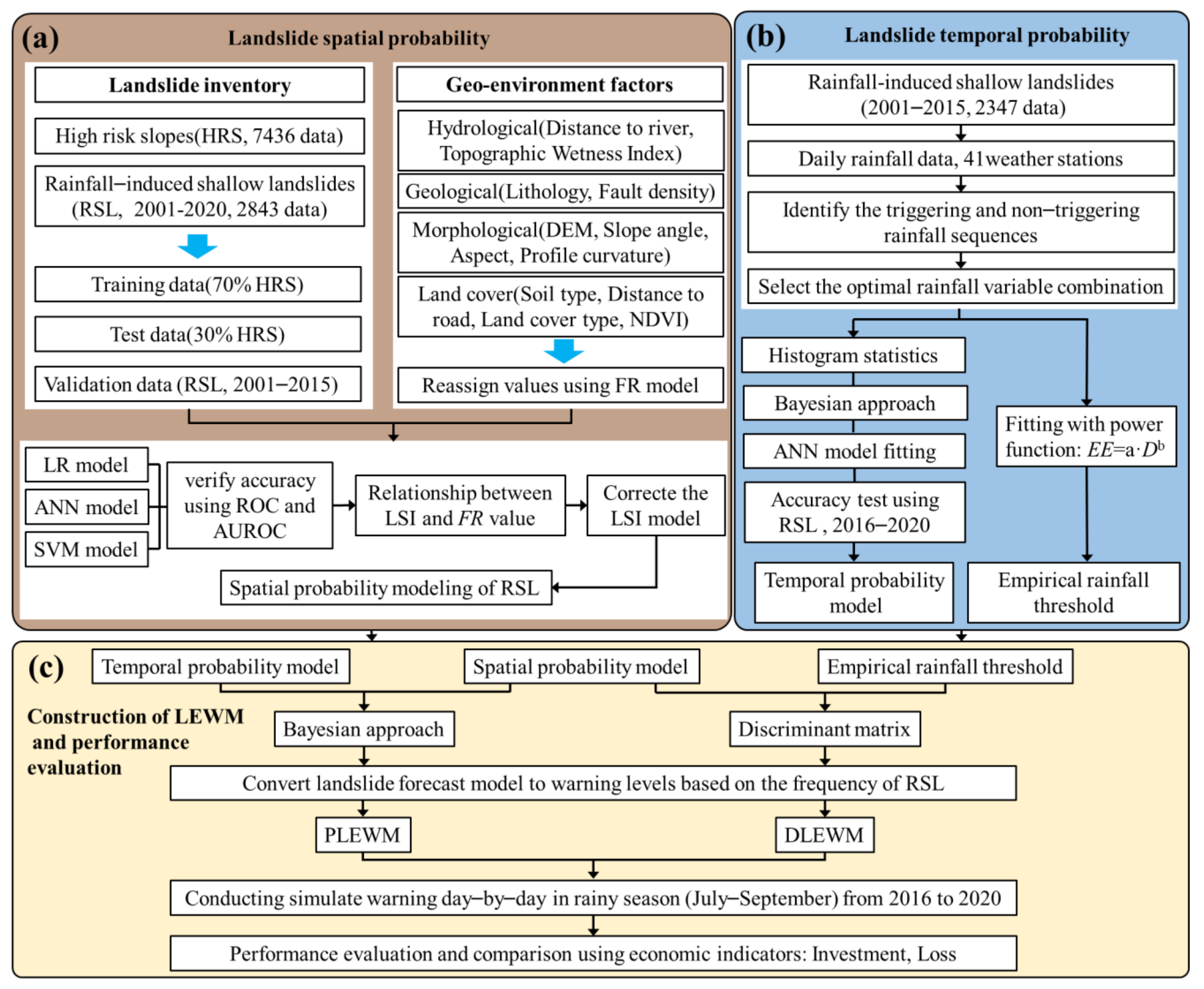
2. Methodology
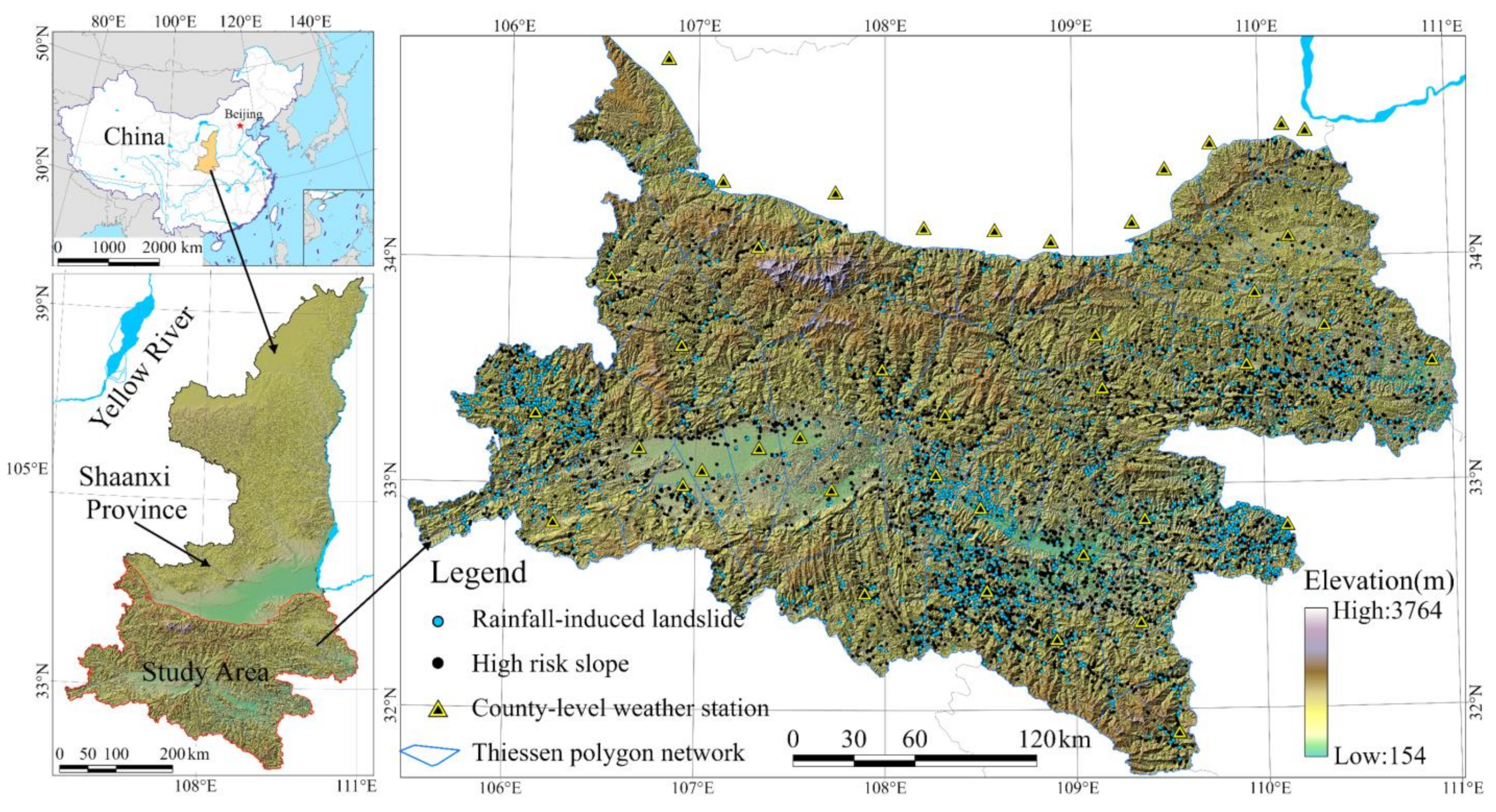
2.1. Introduction to the Qin-Ba Mountain Area
2.2. Construction of the Landslides and Geoenvironmental Factor Database
2.3. Landslide Spatial Probability Model
2.4. Landslide Temporal Probability Model
2.4.1. Identification of Rainfall Events
2.4.2. Effective Rainfall Model
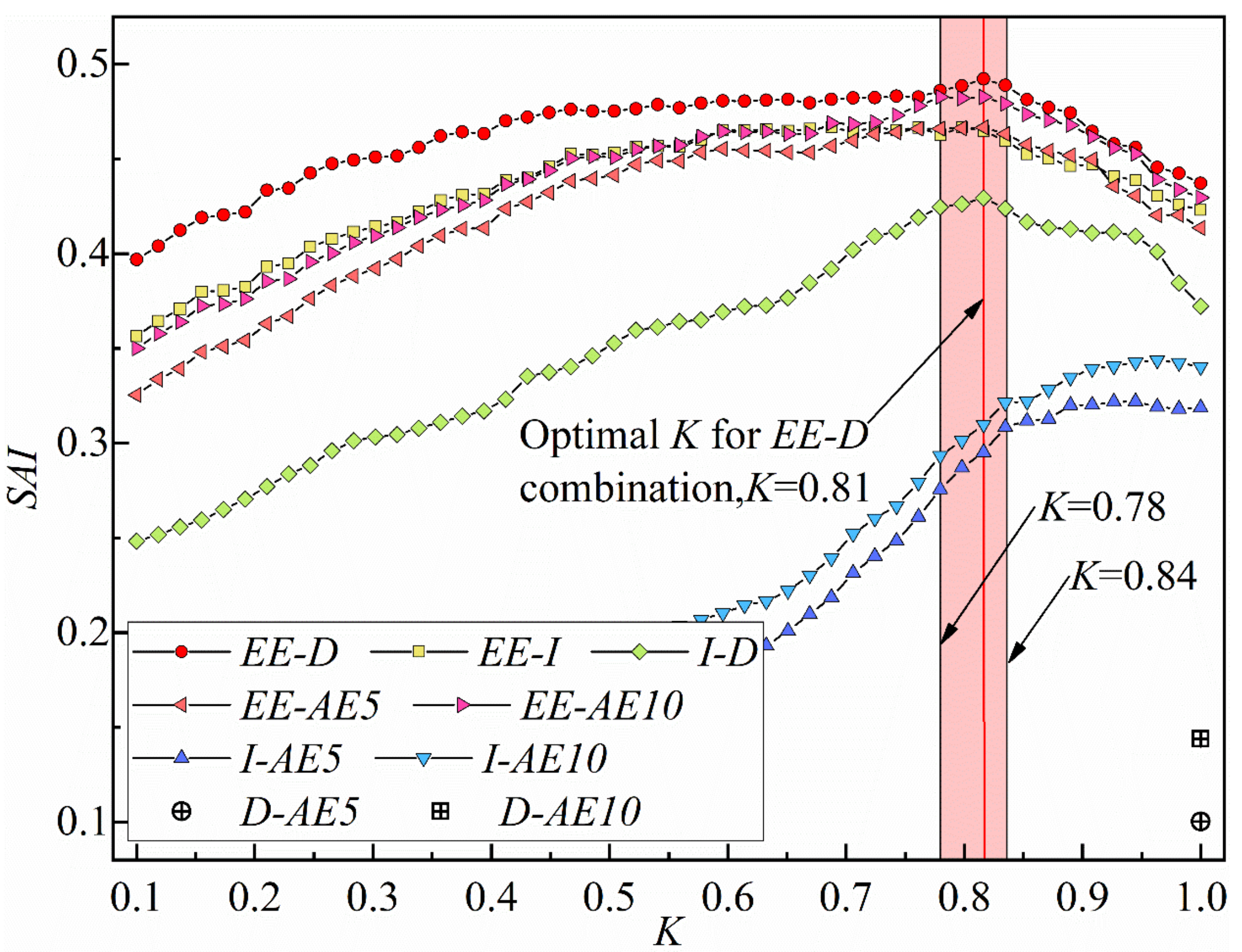
2.4.3. Optimal Rainfall Variable Combination Selection Based on Sensitivity Analysis
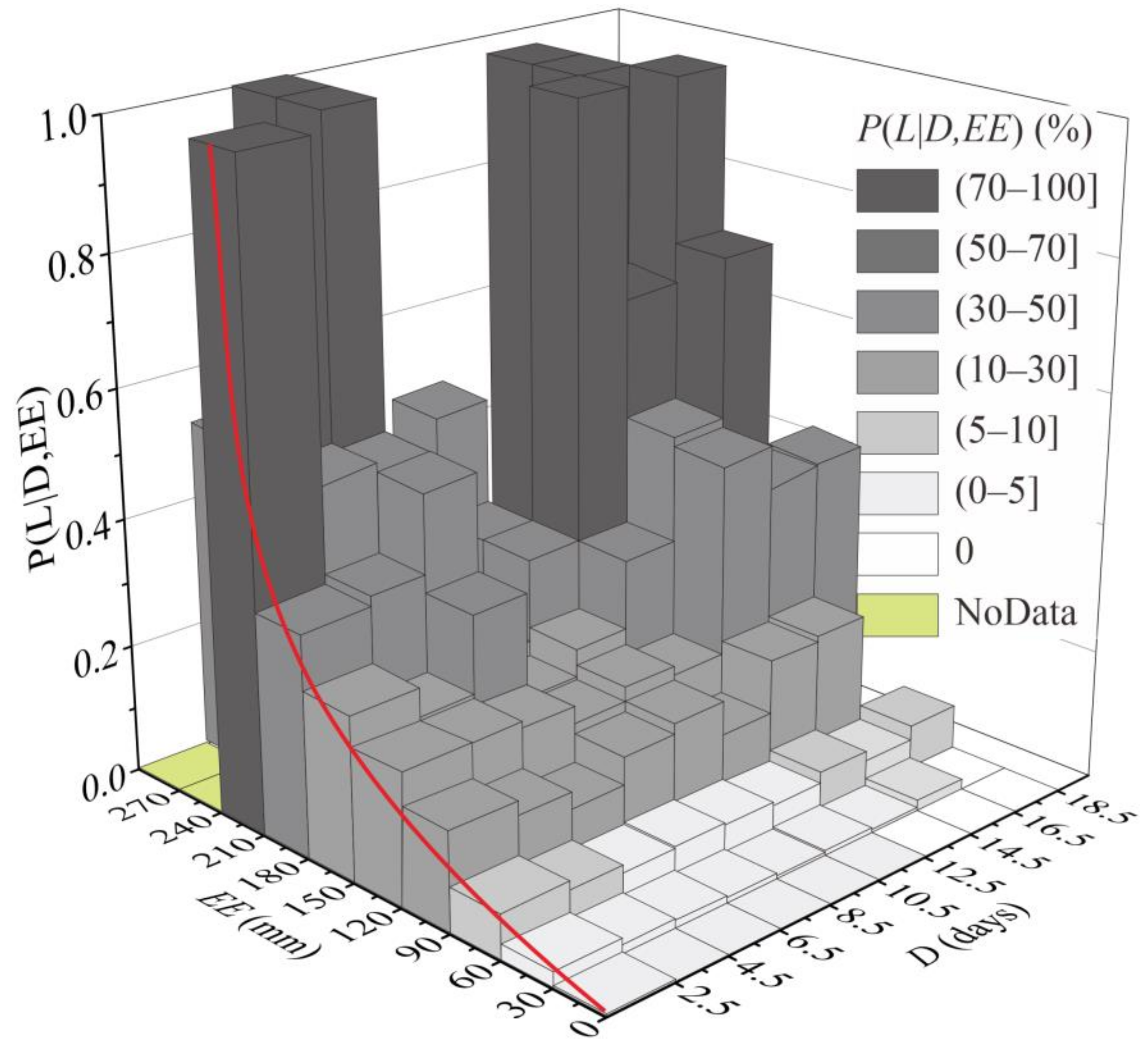
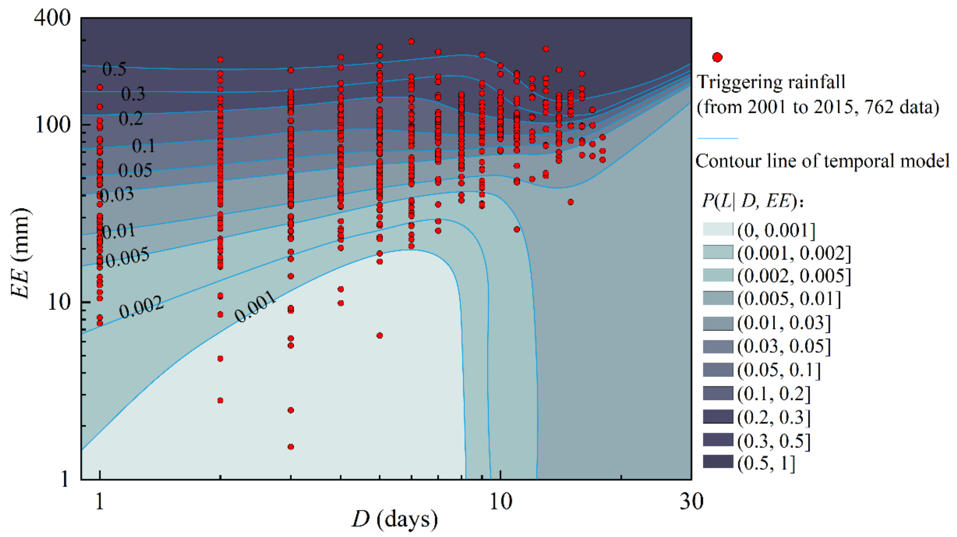
2.4.4. Temporal Probability Model of Landslide Occurrence
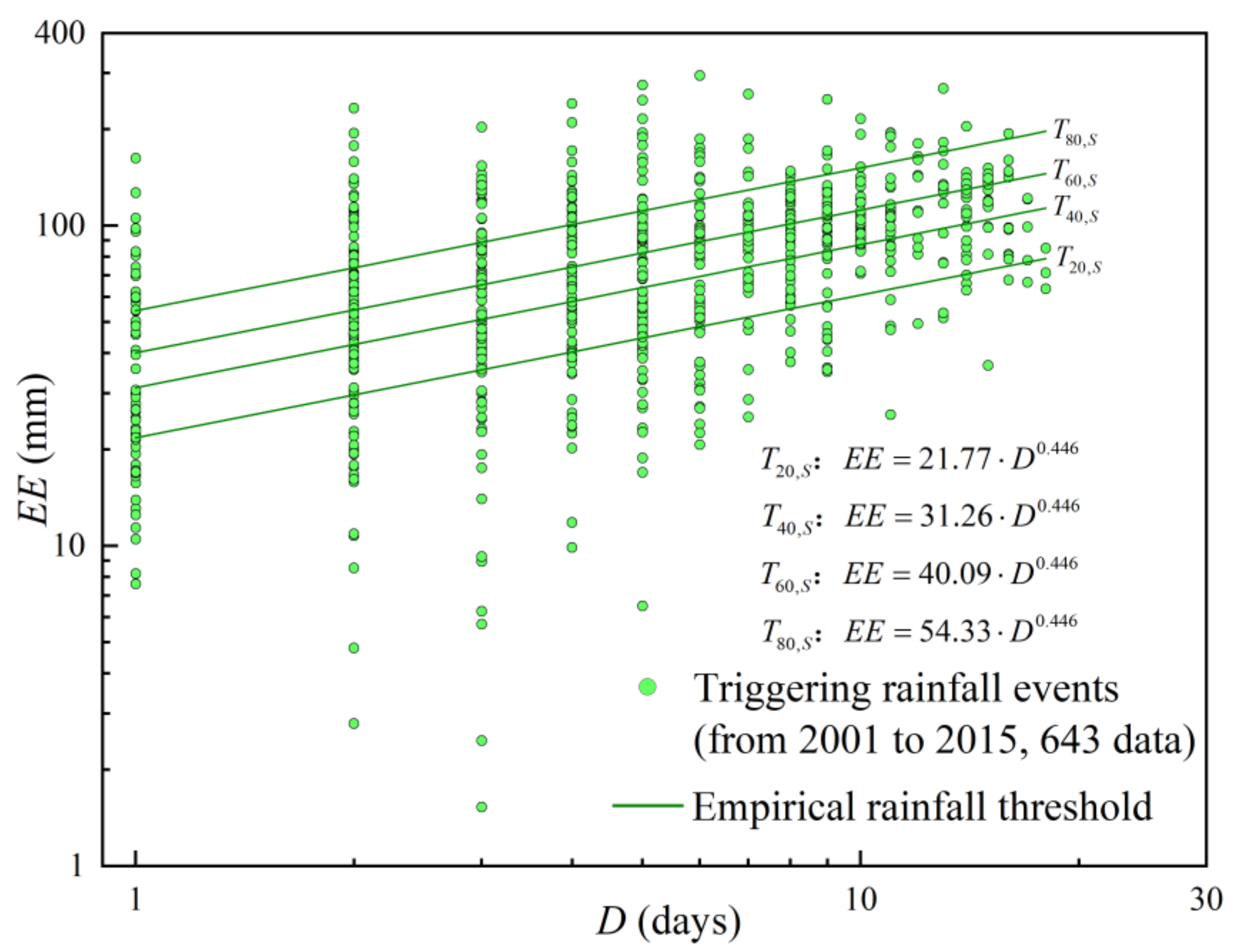
2.4.5. Power-Law-Based Rainfall Threshold
2.5. Landslide Early Warning Model
2.5.1. Probabilistic-Based Landslide Early Warning Model
2.5.2. Discriminant Matrix-Based Landslide Early Warning Model
2.6. Early Warning Model Performance Evaluation
3. Results
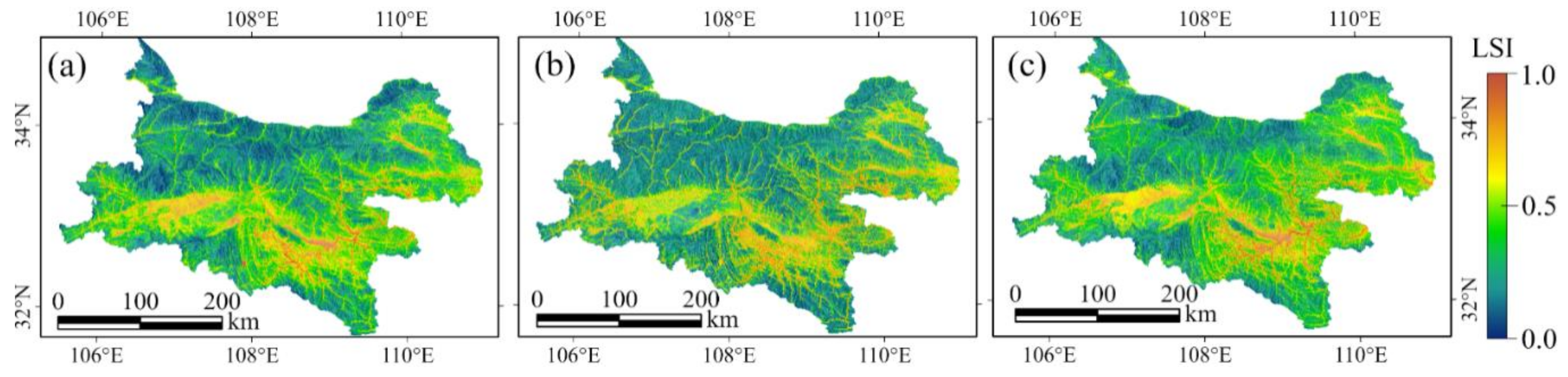
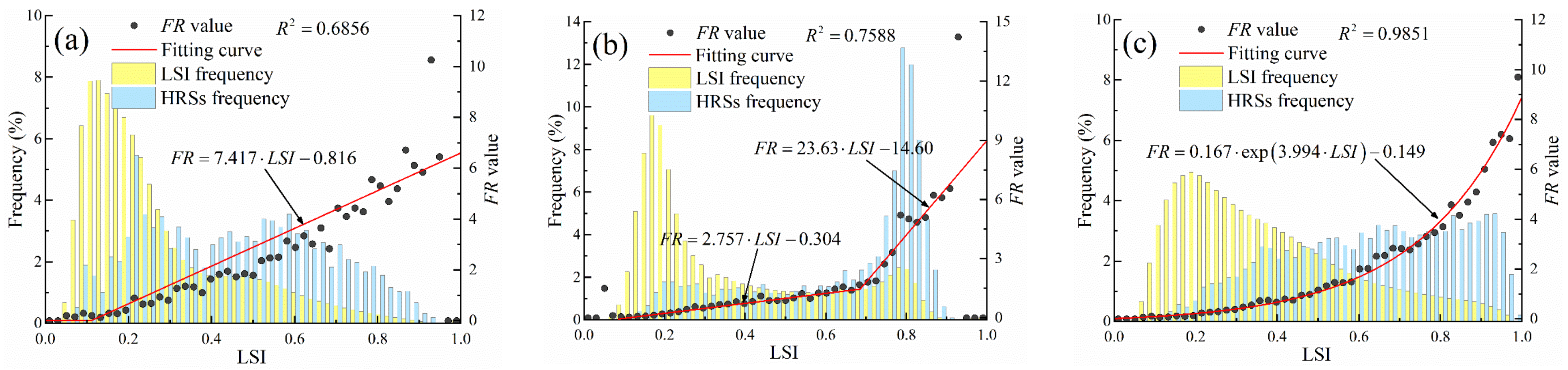
3.1. Landslide Spatial Probability in the Qin-Ba Mountain Area
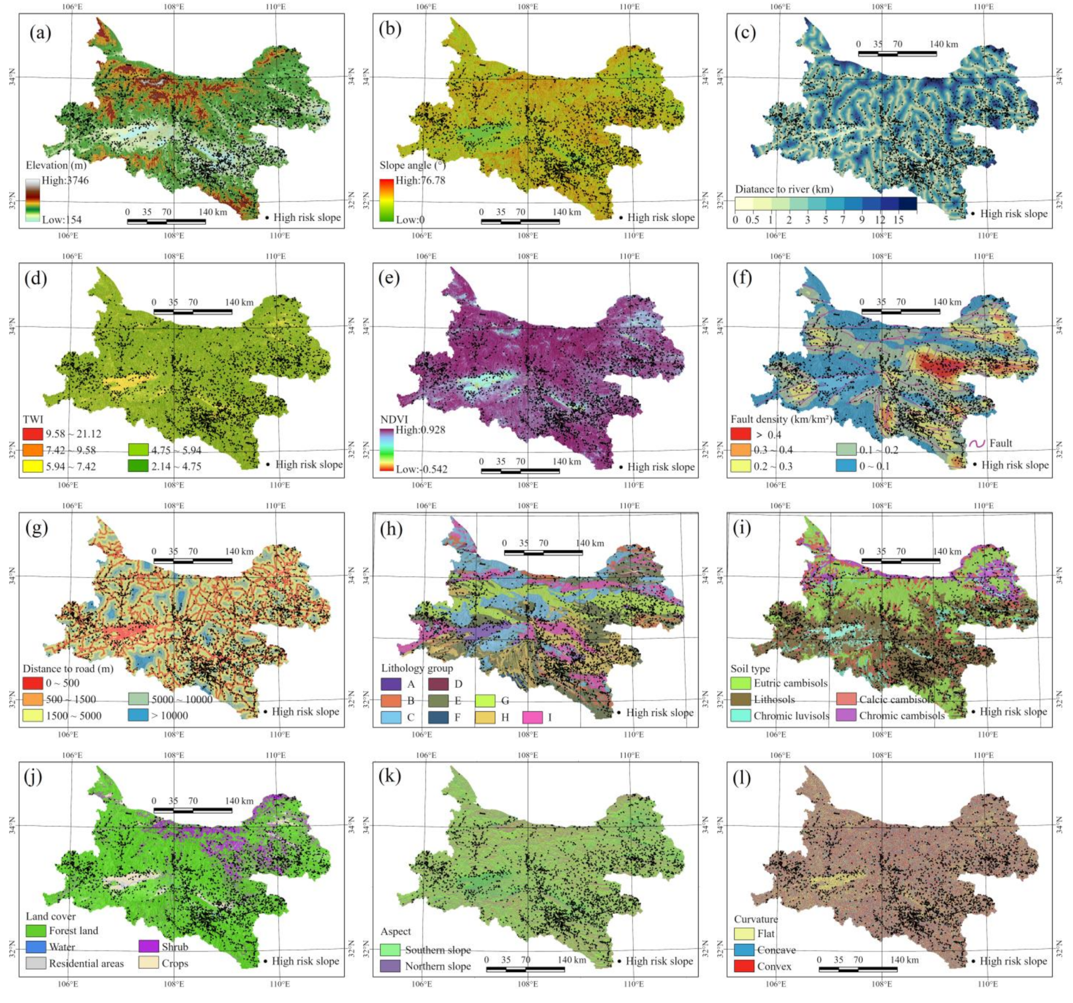
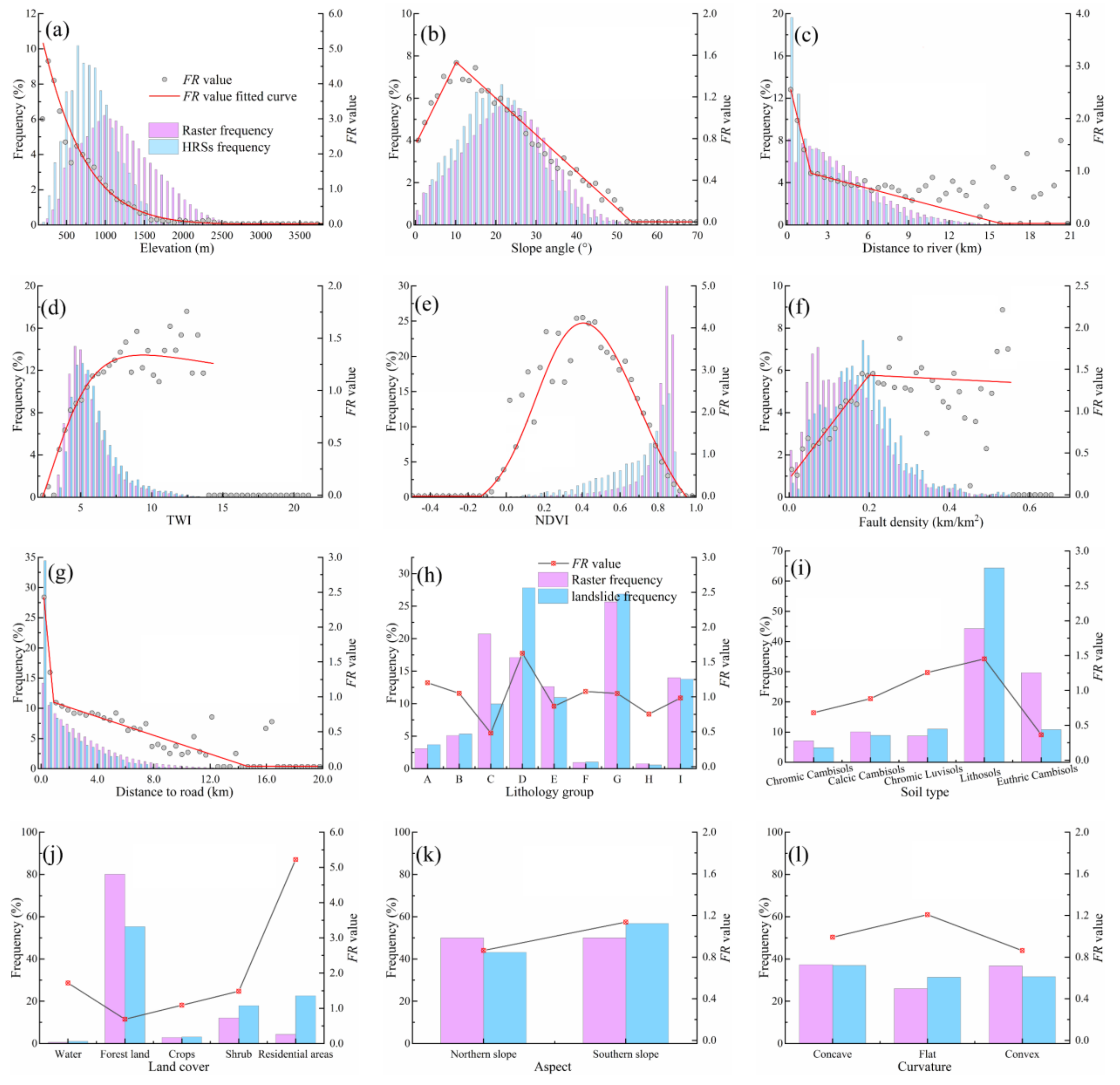
3.1.1. Geoenvironmental Factors and Their Relationship with Landslides
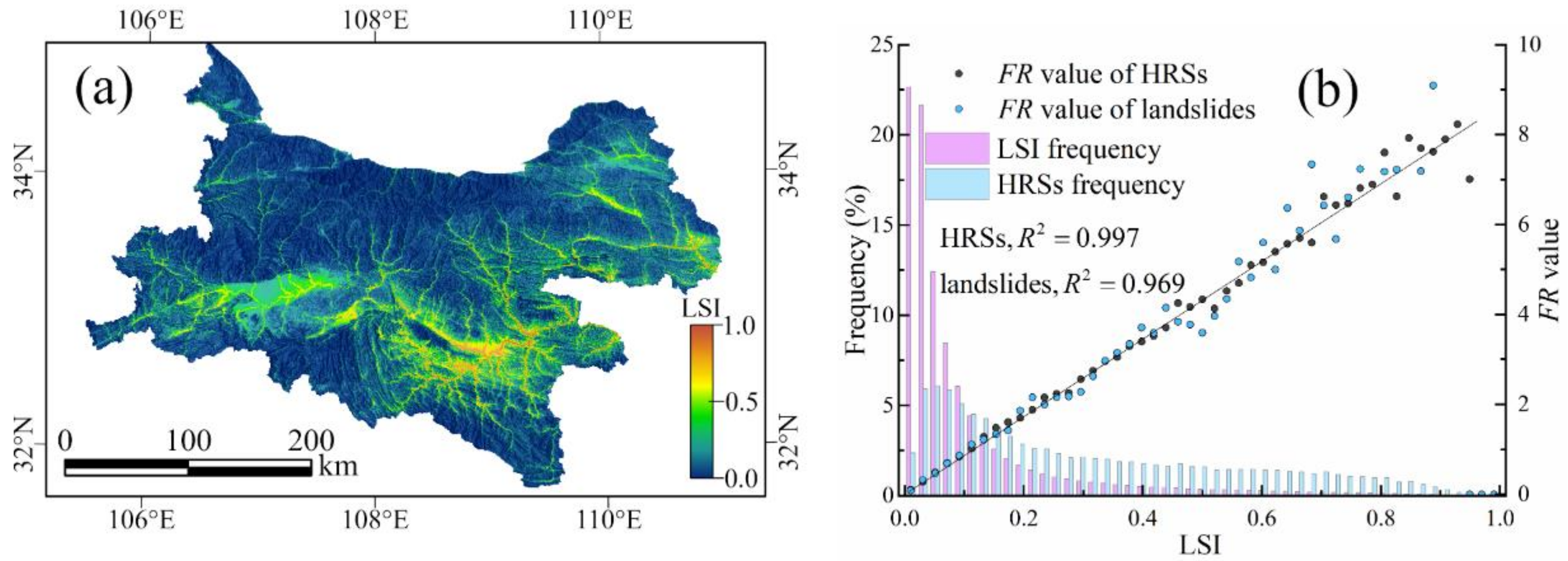
3.1.2. The Spatial Probability of Landslide Occurrence
3.2. Rainfall-Induced Landslide Temporal Probability Model
3.2.1. Selecting the Optimal Combination of Rainfall Variables
3.2.2. Empirical Rainfall Threshold
3.2.3. Temporal Probability Model of Landslide Occurrence
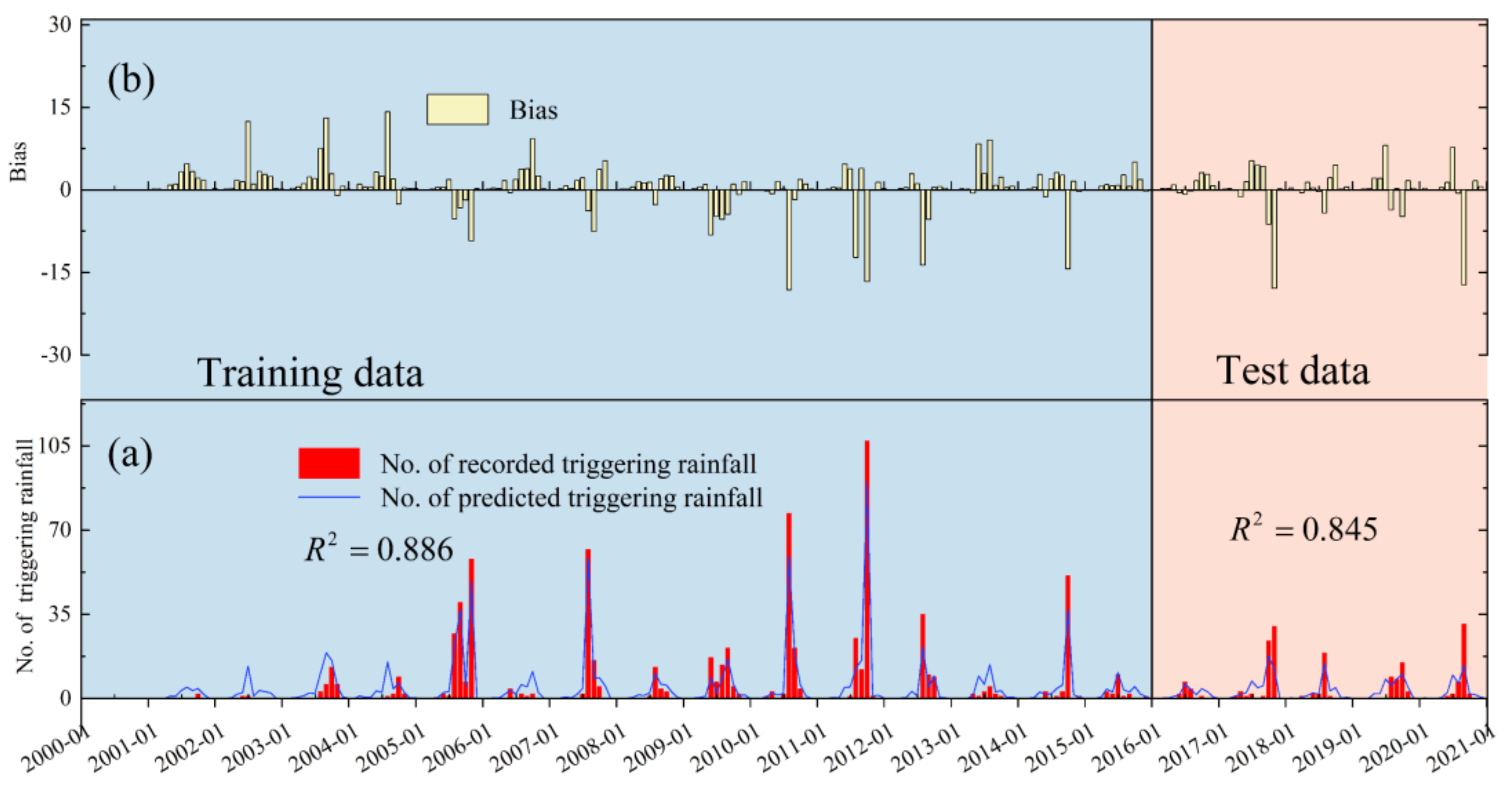
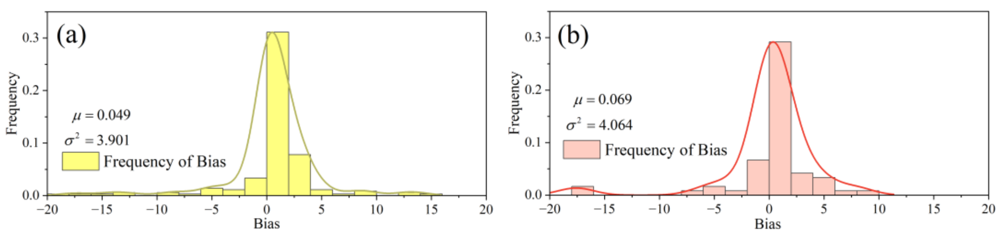
3.2.4. Verification of the Temporal Probability Model
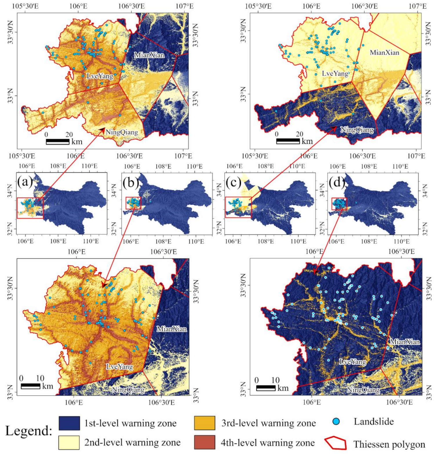
3.3. Warning Strategy
3.3.1. Independence Test
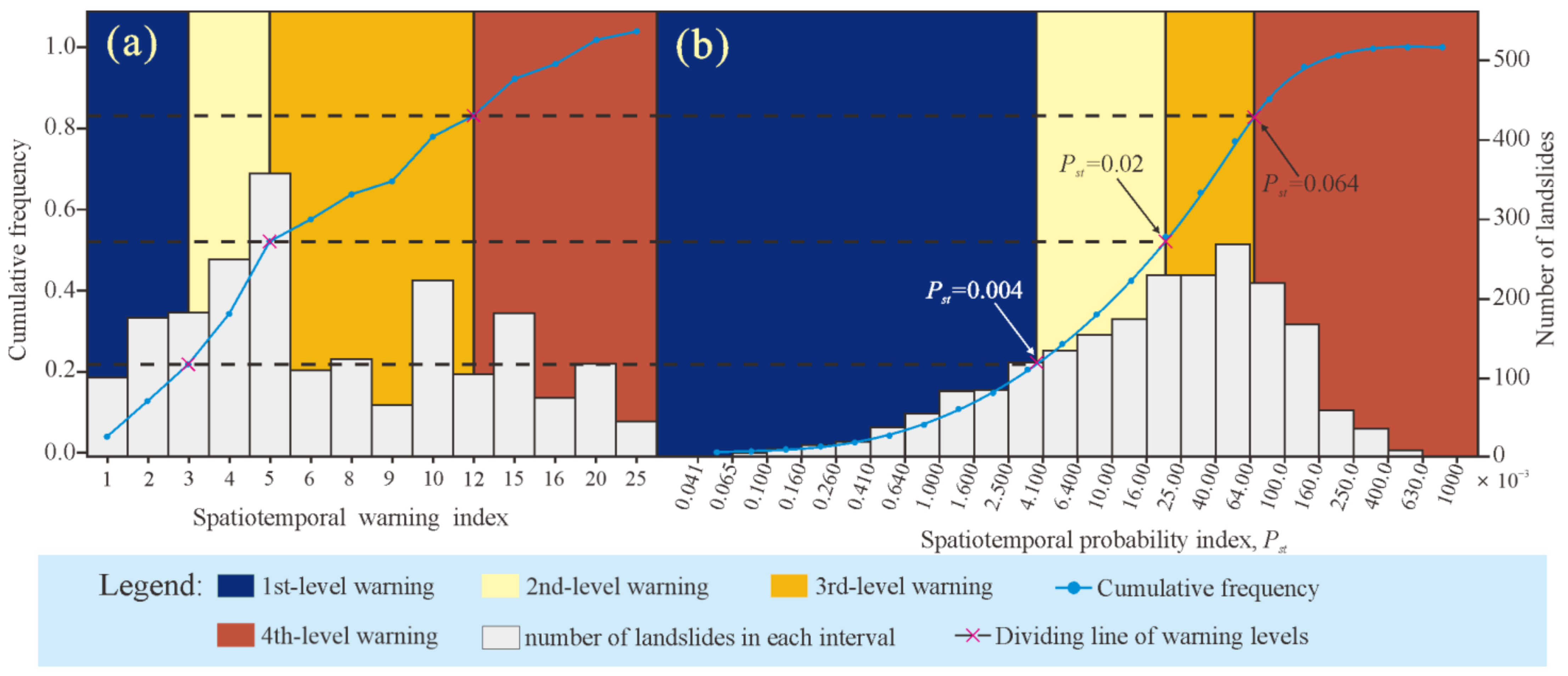
3.3.2. Conversion of the Landslide Forecast Model to Warning Levels
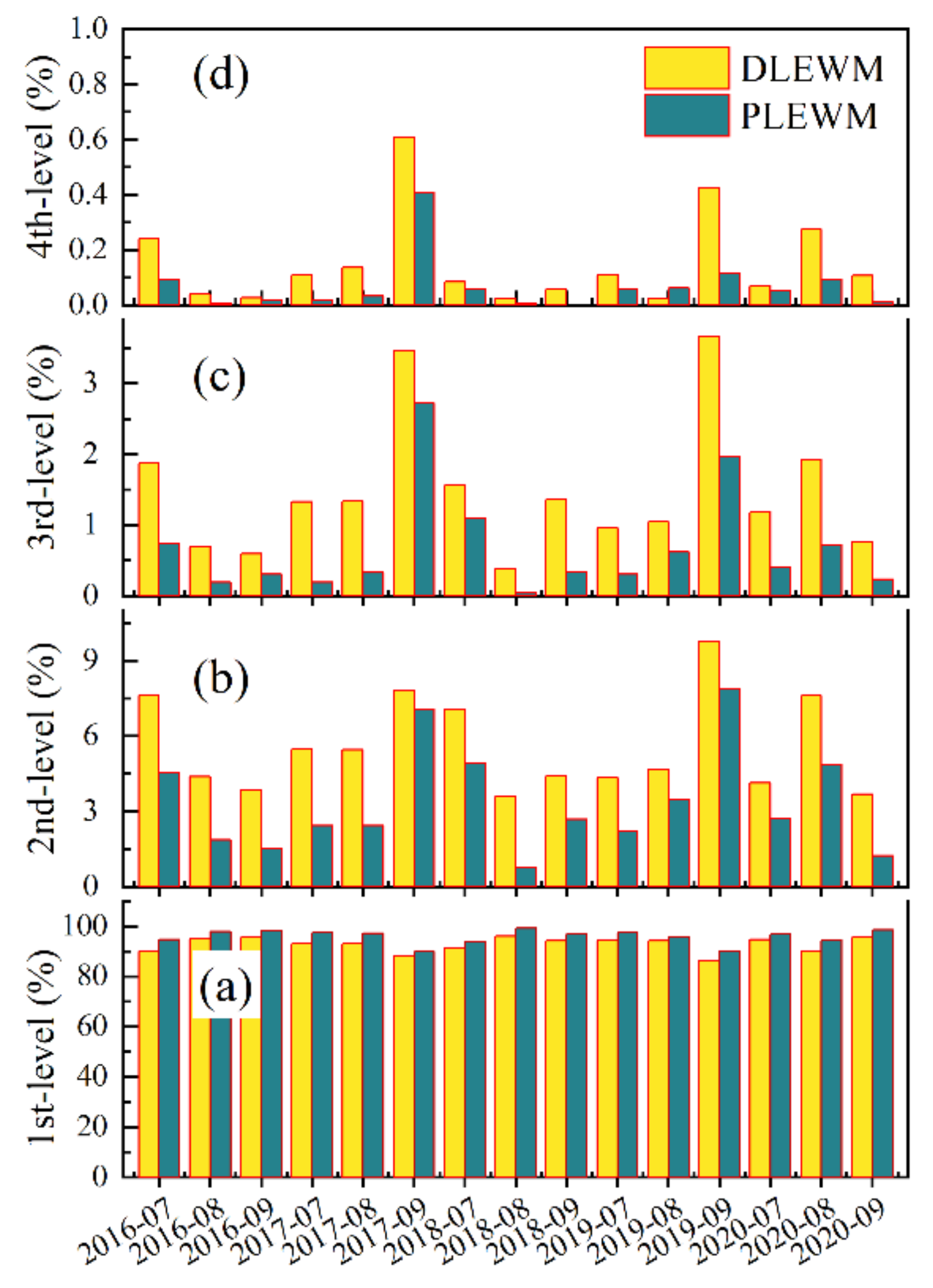
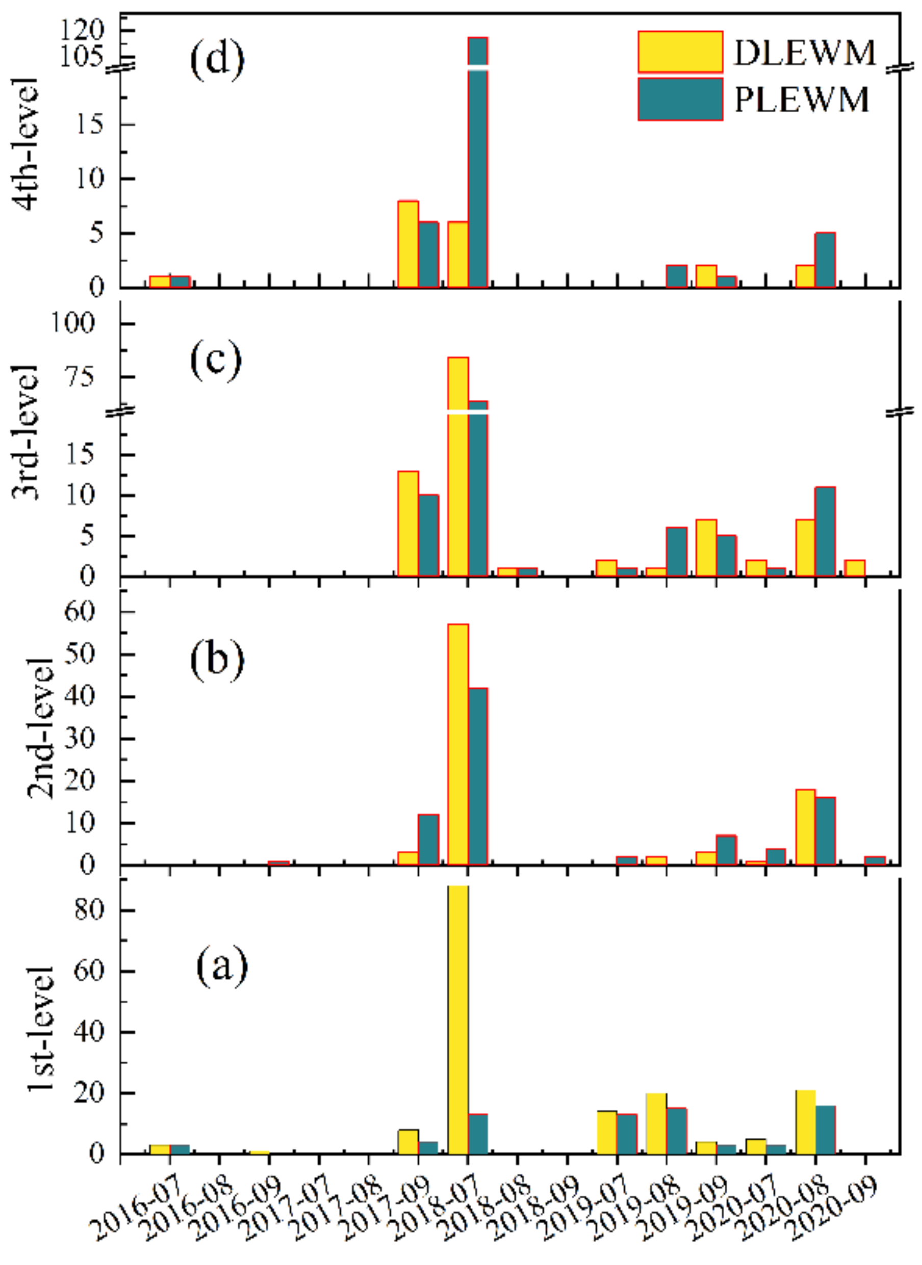
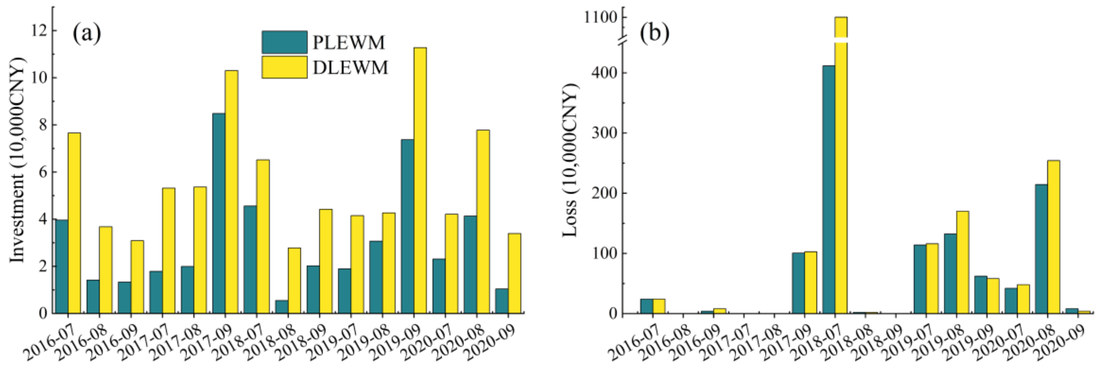
3.4. Simulated Warning Using the PLEWM and DLEWM
4. Discussion
4.1. Spatial Probability Model of Landslide Occurrence
4.2. The PLEWM or DLEWM in Practical Applications?
4.3. Performance Evaluation of the LEWM
5. Conclusions
Supplementary Materials
Author Contributions
Funding
Data Availability Statement
Acknowledgments
Conflicts of Interest
Abbreviations
| Abbreviation | Description | Variable | Description |
| LEWM | Landslide early warning model | K | Decay factor in effective rainfall model |
| PLEWM | Probabilistic-based landslide early warning model | Pst | landslide spatiotemporal probability index |
| DLEWM | Discriminate matrix-based landslide early warning model | ET | Cumulative rainfall for automatic detect rainfall events |
| LSI | Landslide susceptibility index | DT | Event duration for automatic detect rainfall events |
| FR | Frequency ratio value | I | Effective rainfall intensity |
| HRS | High risk slope | D | Rainfall duration |
| RSL | Rainfall induced shallow landslide | E | Cumulative rainfall |
| TWI | Topographic wetness index | EE | Cumulative effective rainfall |
| LR | Logistic regression | AE | Antecedent rainfall |
| SVM | Support vector machine | AE5 | Antecedent rainfall in 5 days |
| ANN | Artificial neural network | AE10 | Antecedent rainfall in 10 days |
| SAI | Sensitivity analysis index | R0 | Rainfall on the day of landslide occurrence |
| S | Landslide spatial probability | Rn | Daily rainfall on the n-th day before landslide occurrence |
| A | Area of the study region | R1 | Rainfall variable 1 |
| CNY | China Yuan | R2 | Rainfall variable 2 |
References
- Wen, B.; Wang, S.; Wang, E.; Zhang, J. Characteristics of rapid giant landslides in China. Landslides 2004, 1, 247–261. [Google Scholar] [CrossRef]
- Petley, D. Global patterns of loss of life from landslides. Geology 2012, 40, 927–930. [Google Scholar] [CrossRef]
- Fan, W.; Wei, X.-S.; Cao, Y.-B.; Zheng, B. Landslide susceptibility assessment using the certainty factor and analytic hierarchy process. J. Mt. Sci. 2017, 14, 906–925. [Google Scholar] [CrossRef]
- Froude, M.J.; Petley, D.N. Global fatal landslide occurrence from 2004 to 2016. Nat. Hazards Earth Syst. Sci. 2018, 18, 2161–2181. [Google Scholar] [CrossRef] [Green Version]
- Wilson, R. The Rise and Fall of a Debris-Flow Warning System for the San Francisco Bay Region, California. Landslide Hazard Risk 2005, 17, 493–516. [Google Scholar] [CrossRef]
- Guzzetti, F.; Gariano, S.L.; Peruccacci, S.; Brunetti, M.T.; Marchesini, I.; Rossi, M.; Melillo, M. Geographical landslide early warning systems. Earth-Sci. Rev. 2020, 200, 102973. [Google Scholar] [CrossRef]
- Calvello, M.; Piciullo, L. Assessing the performance of regional landslide early warning models: The EDuMaP method. Nat. Hazards Earth Syst. Sci. 2016, 16, 103–122. [Google Scholar] [CrossRef] [Green Version]
- UNISDR. Developing early warning systems: A checklist. In Proceedings of the Third International Conference on Early Warning (EWC III), Bonn, Germany, 27–29 March 2006; pp. 27–29. [Google Scholar]
- Intrieri, E.; Gigli, G.; Casagli, N.; Nadim, F. Brief communication “Landslide Early Warning System: Toolbox and general concepts”. Nat. Hazards Earth Syst. Sci. 2013, 13, 85–90. [Google Scholar] [CrossRef] [Green Version]
- Calvello, M.; d’Orsi, R.N.; Piciullo, L.; Paes, N.; Magalhaes, M.; Lacerda, W.A. The Rio de Janeiro early warning system for rainfall-induced landslides: Analysis of performance for the years 2010–2013. Int. J. Disaster Risk Reduct. 2015, 12, 3–15. [Google Scholar] [CrossRef]
- Piciullo, L.; Calvello, M.; Cepeda, J.M. Territorial early warning systems for rainfall-induced landslides. Earth-Sci. Rev. 2018, 179, 228–247. [Google Scholar] [CrossRef]
- Park, J.-Y.; Lee, S.-R.; Lee, D.-H.; Kim, Y.-T.; Lee, J.-S. A regional-scale landslide early warning methodology applying statistical and physically based approaches in sequence. Eng. Geol. 2019, 260, 5193. [Google Scholar] [CrossRef]
- Bordoni, M.; Vivaldi, V.; Lucchelli, L.; Ciabatta, L.; Brocca, L.; Galve, J.P.; Meisina, C. Development of a data-driven model for spatial and temporal shallow landslide probability of occurrence at catchment scale. Landslides 2021, 18, 1209–1229. [Google Scholar] [CrossRef]
- Guzzetti, F.; Peruccacci, S.; Rossi, M.; Stark, C.P. Rainfall thresholds for the initiation of landslides in central and southern Europe. Meteorol. Atmos. Phys. 2007, 98, 239–267. [Google Scholar] [CrossRef]
- Guzzetti, F.; Peruccacci, S.; Rossi, M.; Stark, C.P. The rainfall intensity–duration control of shallow landslides and debris flows: An update. Landslides 2008, 5, 3–17. [Google Scholar] [CrossRef]
- Jaiswal, P.; van Westen, C.J. Estimating temporal probability for landslide initiation along transportation routes based on rainfall thresholds. Geomorphology 2009, 112, 96–105. [Google Scholar] [CrossRef]
- Berti, M.; Martina, M.; Franceschini, S.; Pignone, S.; Simoni, A.; Pizziolo, M. Probabilistic rainfall thresholds for landslide occurrence using a Bayesian approach. J. Geophys. Res. Earth Surf. 2012, 117, 1–20. [Google Scholar] [CrossRef] [Green Version]
- Caine, N. The Rainfall Intensity–Duration Control of Shallow Landslides and Debris Flows. Geogr. Ann. Ser. A Phys. Geogr. 1980, 62, 23–27. [Google Scholar] [CrossRef]
- Aleotti, P. A warning system for rainfall-induced shallow failures. Eng. Geol. 2004, 73, 247–265. [Google Scholar] [CrossRef]
- Brunetti, M.; Peruccacci, S.; Rossi, M.; Luciani, S.; Valigi, D.; Guzzetti, F. Rainfall thresholds for the possible occurrence of landslides in Italy. Nat. Hazards Earth Syst. Sci. 2010, 10, 447–458. [Google Scholar] [CrossRef]
- Peruccacci, S.; Brunetti, M.T.; Luciani, S.; Vennari, C.; Guzzetti, F. Lithological and seasonal control on rainfall thresholds for the possible initiation of landslides in central Italy. Geomorphology 2012, 139–140, 79–90. [Google Scholar] [CrossRef]
- Melillo, M.; Brunetti, M.T.; Peruccacci, S.; Gariano, S.L.; Guzzetti, F. An algorithm for the objective reconstruction of rainfall events responsible for landslides. Landslides 2015, 12, 311–320. [Google Scholar] [CrossRef]
- Rosi, A.; Peternel, T.; Jemec-Auflič, M.; Komac, M.; Segoni, S.; Casagli, N. Rainfall thresholds for rainfall-induced landslides in Slovenia. Landslides 2016, 13, 1571–1577. [Google Scholar] [CrossRef]
- Melillo, M.; Brunetti, M.T.; Peruccacci, S.; Gariano, S.L.; Roccati, A.; Guzzetti, F. A tool for the automatic calculation of rainfall thresholds for landslide occurrence. Environ. Model. Softw. 2018, 105, 230–243. [Google Scholar] [CrossRef]
- Cannon, S.H.; Gartner, J.E.; Wilson, R.C.; Bowers, J.C.; Laber, J.L. Storm rainfall conditions for floods and debris flows from recently burned areas in southwestern Colorado and southern California. Geomorphology 2008, 96, 250–269. [Google Scholar] [CrossRef]
- Giannecchini, R.; Galanti, Y.; D’Amato Avanzi, G.; Barsanti, M. Probabilistic rainfall thresholds for triggering debris flows in a human-modified landscape. Geomorphology 2016, 257, 94–107. [Google Scholar] [CrossRef]
- Frattini, P.; Crosta, G.; Sosio, R. Approaches for defining thresholds and return periods for rainfall-triggered shallow landslides. Hydrol. Processes Int. J. 2009, 23, 1444–1460. [Google Scholar] [CrossRef]
- Robbins, J.C. A probabilistic approach for assessing landslide-triggering event rainfall in Papua New Guinea, using TRMM satellite precipitation estimates. J. Hydrol. 2016, 541, 296–309. [Google Scholar] [CrossRef]
- Glade, T.; Crozier, M.; Smith, P. Applying probability determination to refine landslide-triggering rainfall thresholds using an empirical “Antecedent Daily Rainfall Model”. Pure Appl. Geophys. 2000, 157, 1059–1079. [Google Scholar] [CrossRef]
- Baum, R.L.; Coe, J.A.; Godt, J.W.; Harp, E.L.; Reid, M.E.; Savage, W.Z.; Schulz, W.H.; Brien, D.L.; Chleborad, A.F.; McKenna, J.P.; et al. Regional landslide-hazard assessment for Seattle, Washington, USA. Landslides 2005, 2, 266–279. [Google Scholar] [CrossRef]
- Stähli, M.; Sättele, M.; Huggel, C.; McArdell, B.W.; Lehmann, P.; Van Herwijnen, A.; Berne, A.; Schleiss, M.; Ferrari, A.; Kos, A.; et al. Monitoring and prediction in early warning systems for rapid mass movements. Nat. Hazards Earth Syst. Sci. 2015, 15, 905–917. [Google Scholar] [CrossRef]
- Godt, J.W.; Baum, R.L.; Chleborad, A.F. Rainfall characteristics for shallow landsliding in Seattle, Washington, USA. Earth Surf. Processes Landf. 2006, 31, 97–110. [Google Scholar] [CrossRef]
- Baum, R.L.; Godt, J.W. Early warning of rainfall-induced shallow landslides and debris flows in the USA. Landslides 2010, 7, 259–272. [Google Scholar] [CrossRef]
- Rosi, A.; Lagomarsino, D.; Rossi, G.; Segoni, S.; Battistini, A.; Casagli, N. Updating EWS rainfall thresholds for the triggering of landslides. Nat. Hazards 2015, 78, 297–308. [Google Scholar] [CrossRef]
- Guzzetti, F.; Reichenbach, P.; Cardinali, M.; Galli, M.; Ardizzone, F. Probabilistic landslide hazard assessment at the basin scale. Geomorphology 2005, 72, 272–299. [Google Scholar] [CrossRef]
- Skilodimou, H.D.; Bathrellos, G.D.; Koskeridou, E.; Soukis, K.; Rozos, D. Physical and Anthropogenic Factors Related to Landslide Activity in the Northern Peloponnese, Greece. Land 2018, 7, 85. [Google Scholar] [CrossRef] [Green Version]
- Bathrellos, G.D.; Skilodimou, H.D. Land Use Planning for Natural Hazards. Land 2019, 8, 128. [Google Scholar] [CrossRef] [Green Version]
- Liu, S.; Yin, K.; Zhou, C.; Gui, L.; Liang, X.; Lin, W.; Zhao, B. Susceptibility Assessment for Landslide Initiated along Power Transmission Lines. Remote Sens. 2021, 13, 5068. [Google Scholar] [CrossRef]
- Skilodimou, H.D.; Bathrellos, G.D. Natural and Technological Hazards in Urban Areas: Assessment, Planning and Solutions. Sustainability 2021, 13, 8301. [Google Scholar] [CrossRef]
- Yin, K.; Chen, L.; Zhang, G. Regional Landslide Hazard Warning and Risk Assessment. Earth Sci. Front. 2007, 14, 85–93. [Google Scholar] [CrossRef]
- Zhang, G.; Chen, L.; Dong, Z. Real-Time Warning System of Regional Landslides Supported by WEBGIS and its Application in Zhejiang Province, China. Procedia Earth Planet. Sci. 2011, 2, 247–254. [Google Scholar] [CrossRef]
- Piciullo, L.; Gariano, S.L.; Melillo, M.; Brunetti, M.T.; Peruccacci, S.; Guzzetti, F.; Calvello, M. Definition and performance of a threshold-based regional early warning model for rainfall-induced landslides. Landslides 2017, 14, 995–1008. [Google Scholar] [CrossRef]
- Krøgli, I.K.; Devoli, G.; Colleuille, H.; Boje, S.; Sund, M.; Engen, I.K. The Norwegian forecasting and warning service for rainfall- and snowmelt-induced landslides. Nat. Hazards Earth Syst. Sci. 2018, 18, 1427–1450. [Google Scholar] [CrossRef] [Green Version]
- Palau, R.M.; Berenguer, M.; Hürlimann, M.; Sempere-Torres, D. Application of a fuzzy verification framework for the evaluation of a regional-scale landslide early warning system during the January 2020 Gloria storm in Catalonia (NE Spain). Landslides 2022, 19, 1599–1616. [Google Scholar] [CrossRef]
- Reichenbach, P.; Rossi, M.; Malamud, B.D.; Mihir, M.; Guzzetti, F. A review of statistically-based landslide susceptibility models. Earth-Sci. Rev. 2018, 180, 60–91. [Google Scholar] [CrossRef]
- Merghadi, A.; Yunus, A.P.; Dou, J.; Whiteley, J.; ThaiPham, B.; Bui, D.T.; Avtar, R.; Abderrahmane, B. Machine learning methods for landslide susceptibility studies: A comparative overview of algorithm performance. Earth-Sci. Rev. 2020, 207, 103225. [Google Scholar] [CrossRef]
- Ali, S.A.; Parvin, F.; Vojteková, J.; Costache, R.; Linh, N.T.T.; Pham, Q.B.; Vojtek, M.; Gigović, L.; Ahmad, A.; Ghorbani, M.A. GIS-based landslide susceptibility modeling: A comparison between fuzzy multi-criteria and machine learning algorithms. Geosci. Front. 2021, 12, 857–876. [Google Scholar] [CrossRef]
- Kawagoe, S.; Kazama, S.; Sarukkalige, P.R. Probabilistic modelling of rainfall induced landslide hazard assessment. Hydrol. Earth Syst. Sci. 2010, 14, 1047–1061. [Google Scholar] [CrossRef] [Green Version]
- Tiranti, D.; Nicolò, G.; Gaeta, A.R. Shallow landslides predisposing and triggering factors in developing a regional early warning system. Landslides 2019, 16, 235–251. [Google Scholar] [CrossRef]
- Piciullo, L.; Tiranti, D.; Pecoraro, G.; Cepeda, J.M.; Calvello, M. Standards for the performance assessment of territorial landslide early warning systems. Landslides 2020, 17, 2533–2546. [Google Scholar] [CrossRef]
- Giannecchini, R.; Galanti, Y.; D’Amato Avanzi, G. Critical rainfall thresholds for triggering shallow landslides in the Serchio River Valley (Tuscany, Italy). Nat. Hazards Earth Syst. Sci. 2012, 12, 829–842. [Google Scholar] [CrossRef]
- Martelloni, G.; Segoni, S.; Fanti, R.; Catani, F. Rainfall thresholds for the forecasting of landslide occurrence at regional scale. Landslides 2012, 9, 485–495. [Google Scholar] [CrossRef] [Green Version]
- Staley, D.M.; Kean, J.W.; Cannon, S.H.; Schmidt, K.M.; Laber, J.L. Objective definition of rainfall intensity–duration thresholds for the initiation of post-fire debris flows in southern California. Landslides 2013, 10, 547–562. [Google Scholar] [CrossRef]
- Peres, D.J.; Cancelliere, A. Derivation and evaluation of landslide-triggering thresholds by a Monte Carlo approach. Hydrol. Earth Syst. Sci. 2014, 18, 4913–4931. [Google Scholar] [CrossRef] [Green Version]
- Piciullo, L.; Dahl, M.P.; Devoli, G.; Colleuille, H.; Calvello, M. Adapting the EDuMaP method to test the performance of the Norwegian early warning system for weather-induced landslides. Nat. Hazards Earth Syst. Sci. 2017, 17, 817–831. [Google Scholar] [CrossRef] [Green Version]
- Assilzadeh, H.; Levy, J.K.; Wang, X. Landslide Catastrophes and Disaster Risk Reduction: A GIS Framework for Landslide Prevention and Management. Remote Sens. 2010, 2, 2259–2273. [Google Scholar] [CrossRef] [Green Version]
- Segoni, S.; Piciullo, L.; Gariano, S.L. A review of the recent literature on rainfall thresholds for landslide occurrence. Landslides 2018, 15, 1483–1501. [Google Scholar] [CrossRef]
- Rogers, D.; Tsirkunov, V.; Costs and Benefits of Early Warning Systems. Global Assessment Report. 2011. Available online: http://documents1.worldbank.org/curated/pt/609951468330279598/pdf/693580ESW0P1230aster0Risk0Reduction.pdf (accessed on 1 July 2022).
- Alfieri, L.; Salamon, P.; Pappenberger, F.; Wetterhall, F.; Thielen, J. Operational early warning systems for water-related hazards in Europe. Environ. Sci. Policy 2012, 21, 35–49. [Google Scholar] [CrossRef]
- Glade, T.; Nadim, F. Early warning systems for natural hazards and risks. Nat. Hazards 2014, 70, 1669–1671. [Google Scholar] [CrossRef] [Green Version]
- United Nations Office for Disaster Risk Reduction. Sendai framework for disaster risk reduction 2015–2030. In Proceedings of the 3rd United Nations World Conference on DRR, Sendai, Japan, 14–18 March 2015; Available online: https://www.undrr.org/publication/sendai-framework-disaster-risk-reduction-2015-2030 (accessed on 1 July 2022).
- Dai, F.; Lee, C.; Ngai, Y.Y. Landslide risk assessment and management: An overview. Eng. Geol. 2002, 64, 65–87. [Google Scholar] [CrossRef]
- Fell, R.; Corominas, J.; Bonnard, C.; Cascini, L.; Leroi, E.; Savage, W.Z. Guidelines for landslide susceptibility, hazard and risk zoning for land use planning. Eng. Geol. 2008, 102, 85–98. [Google Scholar] [CrossRef]
- Yilmaz, I. Landslide susceptibility mapping using frequency ratio, logistic regression, artificial neural networks and their comparison: A case study from Kat landslides (Tokat—Turkey). Comput. Geosci. 2009, 35, 1125–1138. [Google Scholar] [CrossRef]
- Vessia, G.; Parise, M.; Brunetti, M.T.; Peruccacci, S.; Rossi, M.; Vennari, C.; Guzzetti, F. Automated reconstruction of rainfall events responsible for shallow landslides. Nat. Hazards Earth Syst. Sci. 2014, 14, 2399–2408. [Google Scholar] [CrossRef] [Green Version]
- Achour, Y.; Pourghasemi, H.R. How do machine learning techniques help in increasing accuracy of landslide susceptibility maps? Geosci. Front. 2020, 11, 871–883. [Google Scholar] [CrossRef]
- Guo, Z.; Shi, Y.; Huang, F.; Fan, X.; Huang, J. Landslide susceptibility zonation method based on C5.0 decision tree and K-means cluster algorithms to improve the efficiency of risk management. Geosci. Front. 2021, 12, 101249. [Google Scholar] [CrossRef]
- Huang, F.; Chen, J.; Liu, W.; Huang, J.; Hong, H.; Chen, W. Regional rainfall-induced landslide hazard warning based on landslide susceptibility mapping and a critical rainfall threshold. Geomorphology 2022, 408, 108236. [Google Scholar] [CrossRef]
- Ma, T.; Li, C.; Lu, Z.; Wang, B. An effective antecedent precipitation model derived from the power-law relationship between landslide occurrence and rainfall level. Geomorphology 2014, 216, 187–192. [Google Scholar] [CrossRef]
- Iadanza, C.; Trigila, A.; Napolitano, F. Identification and characterization of rainfall events responsible for triggering of debris flows and shallow landslides. J. Hydrol. 2016, 541, 230–245. [Google Scholar] [CrossRef]
- Jiang, Z.; Fan, X.; Siva Subramanian, S.; Yang, F.; Tang, R.; Xu, Q.; Huang, R. Probabilistic rainfall thresholds for debris flows occurred after the Wenchuan earthquake using a Bayesian technique. Eng. Geol. 2021, 280, 105965. [Google Scholar] [CrossRef]
- Li, C.; Ma, T.; Zhu, X.; Li, W. The power–law relationship between landslide occurrence and rainfall level. Geomorphology 2011, 130, 221–229. [Google Scholar] [CrossRef]
- Ma, T.; Li, C.; Lu, Z.; Bao, Q. Rainfall intensity–duration thresholds for the initiation of landslides in Zhejiang Province, China. Geomorphology 2015, 245, 193–206. [Google Scholar] [CrossRef]
- Martinotti, M.E.; Pisano, L.; Marchesini, I.; Rossi, M.; Peruccacci, S.; Brunetti, M.T.; Melillo, M.; Amoruso, G.; Loiacono, P.; Vennari, C.; et al. Landslides, floods and sinkholes in a karst environment: The 1–6 September 2014 Gargano event, southern Italy. Nat. Hazards Earth Syst. Sci. 2017, 17, 467–480. [Google Scholar] [CrossRef] [Green Version]
- Fenwick, D.; Scheidt, C.; Caers, J. Quantifying Asymmetric Parameter Interactions in Sensitivity Analysis: Application to Reservoir Modeling. Math. Geosci. 2014, 46, 493–511. [Google Scholar] [CrossRef]
- He, J.; Qiu, H.; Qu, F.; Hu, S.; Yang, D.; Shen, Y.; Zhang, Y.; Sun, H.; Cao, M. Prediction of spatiotemporal stability and rainfall threshold of shallow landslides using the TRIGRS and Scoops3D models. Catena 2021, 197, 104999. [Google Scholar] [CrossRef]
- Lee, J.-H.; Kim, H.; Park, H.-J.; Heo, J.-H. Temporal prediction modeling for rainfall-induced shallow landslide hazards using extreme value distribution. Landslides 2020, 18, 321–338. [Google Scholar] [CrossRef]
- Wang, Z.; Wang, D.; Guo, Q.; Wang, D. Regional landslide hazard assessment through integrating susceptibility index and rainfall process. Nat. Hazards 2020, 104, 2153–2173. [Google Scholar] [CrossRef]
- Pedregosa, F.; Varoquaux, G.; Gramfort, A.; Michel, V.; Thirion, B.; Grisel, O.; Blondel, M.; Prettenhofer, P.; Weiss, R.; Dubourg, V. Scikit-learn: Machine learning in Python. J. Mach. Learn. Res. 2011, 12, 2825–2830. Available online: https://jmlr.org/papers/v12/pedregosa11a.html (accessed on 10 November 2021).
- Gariano, S.L.; Brunetti, M.T.; Iovine, G.; Melillo, M.; Peruccacci, S.; Terranova, O.; Vennari, C.; Guzzetti, F. Calibration and validation of rainfall thresholds for shallow landslide forecasting in Sicily, southern Italy. Geomorphology 2015, 228, 653–665. [Google Scholar] [CrossRef]


| Warning Level | Corresponding Measures | Investment (10,000 CNY/A) | Loss (10,000 CNY/Landslide) |
|---|---|---|---|
| 4th-level | There is a great probability of landslide occurrence in the warning zone, and the HRS should be continuously monitored, emergency evacuation routes should be prepared, and residents should be evacuated near the HRS. The dangerous road potentially affected by landslides should be closed. | 8 | 0.1 |
| 3rd-level | Landslides occur with a large probability, and HRS monitoring should be strengthened, residents should be notified to prepare for emergency evacuation, and warning signs should be placed on dangerous roads potentially affected by landslides. | 4 | 2 |
| 2nd-level | Regular monitoring of the HRS, and residents should be notified to report to staff if there is any abnormality in the HRS. | 2 | 4 |
| 1st-level | No preventive measures are needed | 0 | 8 |
| Variable Combination | D | I | EE | AE5 | AE10 |
|---|---|---|---|---|---|
| D | - | I-D | D-EE | D-AE5 | D-AE10 |
| I | - | - | I-EE | I-AE5 | I-AE10 |
| EE | - | - | - | EE-AE5 | EE-AE10 |
| Warning Levels | S1 (0–0.2) | S2 (0.2–0.4) | S3 (0.4–0.6) | S4 (0.6–0.8) | S5 (0.8–1.0) |
|---|---|---|---|---|---|
| T1 (<20%) | 1st-level warning | 1st-level warning | 1st-level warning | 2nd-level warning | 2nd-level warning |
| T2 (20–40%) | 1st-level warning | 2nd-level warning | 3rd-level warning | 3rd-level warning | 3rd-level warning |
| T3 (40–60%) | 1st-level warning | 3rd-level warning | 3rd-level warning | 3rd-level warning | 4th-level warning |
| T4 (60–80%) | 2nd-level warning | 3rd-level warning | 3rd-level warning | 4th-level warning | 4th-level warning |
| T5 (>80%) | 2nd-level warning | 3rd-level warning | 4th-level warning | 4th-level warning | 4th-level warning |
| Symbol | Performance Indicator | DLEWM | PLEWM | Description or Formula |
|---|---|---|---|---|
| LP | Potential losses | 3088 | 3088 | losses caused by landslides if no warning information is given, which is calculated based on Table 1. |
| L | Loss | 1887.9 | 1115.1 | Losses caused by landslides with the help of warning information |
| Inv | Investment | 84.16 | 45.90 | Cost inputs required for the response measures |
| Eff | Effectiveness | 1200.1 | 1972.9 | Mitigated losses, LP − L |
| ER | Effectiveness rate | 0.3886 | 0.6389 | E/LP |
| ECW | Effectiveness of correct warning | 844.8 | 1558 | Losses mitigated in case of correct warning |
| ERCA | Effectiveness rate of correct warning | 0.2736 | 0.5045 | ECW/LP |
| LE | Losses caused by error warning | 1388.7 | 780.5 | Losses caused by missed and false warning |
| LER | Loss rate of error waning | 0.4497 | 0.2528 | LE/LP |
| CE | Total cost-effectiveness | 35.85 | 151.39 | λ·E − I, here λ is taken as 0.1 |
| CER | Cost-effective conversion rates | 1.4257 | 4.2983 | λ·E/I, here λ is taken as 0.1 |
| CL | Total costs and losses | 272.97 | 157.41 | λ·Loss + I, here λ is taken as 0.1 |
Publisher’s Note: MDPI stays neutral with regard to jurisdictional claims in published maps and institutional affiliations. |
© 2022 by the authors. Licensee MDPI, Basel, Switzerland. This article is an open access article distributed under the terms and conditions of the Creative Commons Attribution (CC BY) license (https://creativecommons.org/licenses/by/4.0/).
Share and Cite
Song, Y.; Fan, W.; Yu, N.; Cao, Y.; Jiang, C.; Chai, X.; Nan, Y. Rainfall Induced Shallow Landslide Temporal Probability Modelling and Early Warning Research in Mountains Areas: A Case Study of Qin-Ba Mountains, Western China. Remote Sens. 2022, 14, 5952. https://doi.org/10.3390/rs14235952
Song Y, Fan W, Yu N, Cao Y, Jiang C, Chai X, Nan Y. Rainfall Induced Shallow Landslide Temporal Probability Modelling and Early Warning Research in Mountains Areas: A Case Study of Qin-Ba Mountains, Western China. Remote Sensing. 2022; 14(23):5952. https://doi.org/10.3390/rs14235952
Chicago/Turabian StyleSong, Yufei, Wen Fan, Ningyu Yu, Yanbo Cao, Chengcheng Jiang, Xiaoqing Chai, and Yalin Nan. 2022. "Rainfall Induced Shallow Landslide Temporal Probability Modelling and Early Warning Research in Mountains Areas: A Case Study of Qin-Ba Mountains, Western China" Remote Sensing 14, no. 23: 5952. https://doi.org/10.3390/rs14235952