Article

High-Resolution Monitoring of the Snow Cover on the Moroccan Atlas through the Spatio-Temporal Fusion of Landsat and Sentinel-2 Images

1
Center for Remote Sensing Applications, Mohammed VI Polytechnic University, Ben Guerir 43150, Morocco
2
Data4Earth Laboratory, Sultan Moulay Slimane University, Beni Mellal 23000, Morocco
3
International Water Research Institute, Mohammed VI Polytechnic University, Ben Guerir 43150, Morocco
*
Author to whom correspondence should be addressed.
Remote Sens. 2022, 14(22), 5814; https://doi.org/10.3390/rs14225814
Submission received: 4 October 2022 / Revised: 2 November 2022 / Accepted: 15 November 2022 / Published: 17 November 2022
(This article belongs to the Special Issue Advances in Remote Sensing of Snow Cover)

Abstract

:
Mapping seasonal snow cover dynamics provides essential information to predict snowmelt during spring and early summer. Such information is vital for water supply management and regulation by national stakeholders. Recent advances in remote sensing have made it possible to reliably estimate and quantify the spatial and temporal variability of snow cover at different scales. However, because of technological constraints, there is a compromise between the temporal, spectral, and spatial resolutions of available satellites. In addition, atmospheric conditions and cloud contamination may increase the number of missing satellite observations. Therefore, data from a single satellite is insufficient to accurately capture snow dynamics, especially in semi-arid areas where snowfall is extremely variable in both time and space. Considering these limitations, the combined use of the next generation of multispectral sensor data from the Landsat-8 (L8) and Sentinel-2 (S2), with a spatial resolution ranging from 10 to 30 m, provides unprecedented opportunities to enhance snow cover mapping. Hence, the purpose of this study is to examine the effectiveness of the combined use of optical sensors through image fusion techniques for capturing snow dynamics and producing detailed and dense normalized difference snow index (NDSI) time series within a semi-arid context. Three different models include the enhanced spatial and temporal adaptive reflectance fusion model (ESTARFM), the flexible spatio-temporal data fusion model (FSDAF), and the pre-classification flexible spatio-temporal data fusion model (pre-classification FSDAF) were tested and compared to merge L8 and S2 data. The results showed that the pre-classification FSDAF model generates the most accurate precise fused NDSI images and retains spatial detail compared to the other models, with the root mean square error (RMSE = 0.12) and the correlation coefficient (R = 0.96). Our results reveal that, the pre-classification FSDAF model provides a high-resolution merged snow time series and can compensate the lack of ground-based snow cover data.

Graphical Abstract

1. Introduction

Snowpack provides a crucial source of water supply for populations and ecosystems by accumulating snow throughout wet winters and releasing it slowly during dry spring and summer [1,2]. Indeed, snow cover is a more important element of the earth’s surface that influences the spatial distribution and conditions of other elements of the cryosphere, as snow is an essential component for glaciers in temperate regions and for maintaining their stability, which affects the global and regional energy budget [3]. Furthermore, snow cover has a direct impact on the environment and socio-economic system, as several investigations indicate that snowmelt water is a major component of runoff systems in downstream areas, in terms of water quantity as well as distribution and water quality [4,5].
Snow cover knowledge has been used for snowmelt and runoff prediction and for the validation or calibration of different hydrological models [6]. In addition, melting snow cover can cause environmental catastrophes such as flooding or droughts in the event of no snow. Therefore, it is necessary to detect in time the beginning of snowmelt to identify eventual flooding [7]. Due to all these aspects and the effect of climate change in mountainous regions on the spatial extent and duration of global snow cover, continuous monitoring of snow cover is one of the most critical topics in the study and understanding of the cryosphere [5].
In semi-arid regions, snow-covered mountain areas are considered water towers, providing a regular source of water for irrigation, drinking water, power generation, dam storage, and a vital buffer during drought periods. Furthermore, water resources from melted snow are the primary source of water for populations living downstream [1] and contribute significantly to groundwater recharge [8,9], and river flows up to 50% in some Moroccan watersheds [10] which fills reservoirs over the wet season.
Despite the significance of the snow-covered area for water resource management in these regions, many gaps remain regarding its fast dynamics in space and time and its characteristics [11,12]. The accurate estimation of snow cover in the High Atlas basins is therefore essential to properly model the overall water balance at the scale of the watershed, and especially the streamflow and groundwater recharge. Moreover, the High Atlas shows a deficiency in terms of meteorological stations [13,14] due to their high cost and the difficulty of accessing the mountainous regions in winter. Additionally, the spatio-temporal variability of the hydroclimate and the complicated topography of the region [15,16,17,18] generate major difficulties for in situ snow cover mapping and monitoring.
As an alternative, optical satellite remote sensing can provide regularly distributed observations in space and time to map snow cover [19,20]. Because of its specific characteristics in the optical part of the electromagnetic spectrum range, snow cover is identifiable through space from different optical sensors [21,22]. The last few years have seen the development of several satellites orbiting the earth that can be used for snow cover monitoring and mapping. Unfortunately, due to technological constraints, existing satellites offer imagery with two options: either data with a long revisit time but high spatial resolution, or data with a short revisit time but low spatial resolution [23,24]. For example, low-resolution and wide swath sensors such as MODIS, SPOT-VEGETATION, and NOAA-AVHRR offer a daily acquisition frequency suitable for temporal monitoring of the earth’s surface at different spatial resolutions varying from 250 m to 1 km. However, the spatial resolution of MODIS is not sufficient to capture snow cover spatial variability, which limits our ability to link the presence or duration of snow cover at the small watershed scale [25,26,27].
MODIS snow product collections was assessed in the rapidly changing snow cover of the arid to semiarid context of the Moroccan Atlas Mountains. Where the results show an overall accuracy of 89%, which was found to be appropriate to characterize the high dynamics of snowpack in this area thanks to its short revisit time of 1 day [14,22]. However, the low spatial resolution of 500 m presented in this product is not sufficient to capture snow cover spatial variability. In addition, it is not efficient enough in capturing the local variability of the snow extent, related to the terrain aspect effect induced by solar radiation as mentioned in previous studies in the same area [13,16].
On the other hand, satellites such as Landsat-8 Operational Land Imager (OLI) provide 30 m spatial resolution images, which is sufficient to monitor land cover changes [28,29], but its 16-day temporal resolution is generally not suitable for monitoring snow cover in mountainous regions due to its high variability during the hydrological year [20,21,30]. In this context, the Copernicus Sentinel-2 mission from the European Space Agency (ESA) consists of two satellites in polar orbit emplaced in the same synchronous orbit, phased at 180° to each other (S2A launched on 23 June 2015, and S2B launched on 7 March 2017). This configuration of two satellites can provide snow cover data every 10 to 5 days with a 10-m spatial resolution [31,32,33].
In recent years, these characteristics of S2 have enabled high spatial resolution monitoring of snow cover in mountain areas [34,35,36]. However, long-term studies have been limited due to the late availability of S2 images. In addition, Gascoin et al. [37] successfully calibrated and approved a basic empirical function for fractional snow cover estimation from only S2 NDSI data at 20 m resolution. Nevertheless, in extremely cloudy locations and despite the 5-day revisit time of S2 data, the frequency of clouds, shadows, and other atmospheric pollutants preclude the ability to visualize the snow cover for several days [22,38,39], which limits the use of only S2 images for snow cover monitoring in the Moroccan Atlas. Moreover, several technological limitations still hamper the use of single satellite sensor systems, in which a trade-off must be achieved to equilibrate revisit time with spatial accuracy and spatial extent. An application such as snow cover monitoring essentially requires high-spatial and high-temporal-resolution images to surmount the limitations caused by clouds thus investigating snow cover dynamics [33,40].
To overcome these limitations and capitalize on the strengths of individual sensors, spatio-temporal fusion (STF) is a spatial remote sensing technique that has emerged as a powerful means of creating new imagery to achieve a dense series with more spatial details and high revisit time [41]. In the past decade, fusion techniques have attracted much interest, and a variety of models have been developed and widely used to monitor the earth’s surface and generate quantitative real-time remote sensing products [42]. Image fusion methods are mainly used to enhance the temporal and spatial resolution of satellite images, as well as the interpretability of input data [43]. In addition, fusion models can be used to solve the issue of data loss due to cloud pollution or shadows in remote sensing image time series [44,45].
Specifically, Gao et al. [24] proposed the spatial and temporal adaptive reflectance fusion model (STARFM) to combine the surface reflectance of Landsat and MODIS. This method produces daily images at high spatial resolution (same resolution as Landsat, i.e., 30 m) using a neighborhood weighting process. Since then, the STARFM became one of the most popular methods used in the literature due to its strong predictive performance and its nature as a pair-based method. STARFM considers the temporal variations of all ground cover categories within a coarse pixel are consistent and comparable. This makes STARFM appropriate for only coherent regions such as large area crop fields [23,46]. To enhance the efficiency of STARFM in inhomogeneous regions, Zhu et al. [47] proposed the enhanced STARFM (ESTARFM), which uses a combination of both coarse and fine image pairs to determine the temporal percentage variation of each category individually, assuming that the proportions of change are constant throughout the period of interest. Later, Zhu et al. [42] proposed a new hybrid technique known as the flexible spatio-temporal data fusion (FSDAF) method that integrates the concepts of the STARFM model and the de-mixing-based techniques using spatial interpolation in one model. The FSDAF method improves the spatiotemporal fusion accuracy in mixed land cover areas with sudden land use changes by employing a single pair of L8 and S2 images at the reference date and a single low-resolution L8 image at the desired prediction date (the fusion date), which greatly reduces the amount of knowledge required for the input and facilitates its implementation [42,48].
The performance and accuracy of STF of remote sensing data are significantly impacted by the choice of the input pair of images [49,50]. Unfortunately, there is no available approach to automatically determine the input pair of images [51]. Several approaches have been used in this context; for example, Zhu et al. [42] used the “nearest date” approach in the FSDAF fusion model they constructed. Peijuan et al. [50] suggested an experimental framework to fuse images where the operator can select one of two strategies: the nearest date or the highest correlation. Liu et al. [49] proposed to use multiple pairs of base images to generate several merged images, and then the weighted total of these merged images was used to obtain the final estimation. On the other hand, Chen et al. [51] have developed a method that quantitatively considers the criteria of “similarity” and “consistency”. The similarity criterion considers that the coarse resolution image at the reference date must be like the one at the estimation date, and the consistency criterion considers that the fine and coarse resolution images at the reference date must be coherent in both geometric and radiometric image properties. Since in this research, we have used the S2 and L8 data, which have significantly similar radiometric and geometric characteristics, for this reason, the use of the second criterion does not give us any differentiation between the pairs of base images used. It is, therefore, important in our case to propose an alternative approach to find the optimal input reference pair of images, which is a key step before the implementation of STF techniques. For this purpose, we proposed using both the similarity criterion and the error quantification criterion between the low-resolution image at the reference date and the one at the merge date. Our suggested approach enhances the prediction precision of fusion techniques by choosing the optimal image pairs used as input to each fusion algorithm.
The STF techniques are an effective solution for generating high spatial resolution images with short time steps to improve the land cover mapping and to enhance the low resolution of the existing remote sensing images for such applications [52,53]. Furthermore, the STF can be an efficient approach to combining satellite imagery with different temporal and spatial resolutions to produce data with high resolution that may be used to create a database for snow cover monitoring and mapping. This enables improved snow cover mapping, which in turn allows for more accurate simulation of water-related parameters such as snowmelt runoff modeling, snow water equivalent estimation, and stream flow prediction.
Following the generation of the fused NDSI image series with high spatial and temporal resolution, the next step is the estimation of the snow cover fraction, considering forest and mountain areas. Indeed, the estimation of the snow cover fraction in forests remains problematic due to the obstruction effects of the forest canopy, which leads to an underestimation of the snow cover area [54]. The forest area is a fundamental element that affects the results of optical satellite snow cover monitoring approaches. However, assessment of these approaches in forest environments is rare because of the lack of reliable in situ snow cover data in these regions [55]. In addition, there are many critical water supply areas with mountain forests, which have significant impacts on the quantity and timing of snowmelt [56]. However, the present study is more concerned with high mountain regions, especially the Moroccan Atlas Mountains (altitude above 4000 m), so the estimation of the snow cover fraction is more dependent on the spatial and temporal resolution of NDSI images.
According to the literature, these methods have been frequently used for monitoring plant cover and phenology [48]. However, their use still should be strongly considered in the study of the snow surface, which also requires high spatial and temporal resolution images to monitor its spatio-temporal dynamics. For all this, the present study builds on those issues and offers the first attempt to use multisource data fusion approaches to increase the revisit time by creating new images and obtaining very dense and detailed snow index time series to enhance the study of snow cover at the Moroccan Atlas scale.
Therefore, the main objective of this study is to evaluate different spatio-temporal fusion models for near-real-time snow cover monitoring and mapping in the Moroccan Atlas basins. This article aims: (i) To produce and assess the merged NDSI at 10 m spatial resolution from S2 and L8 data over the Moroccan Atlas Mountains; (ii) to evaluate the complementarity of L8 and S2 data in monitoring the rapid snow surface dynamics; and (iii) to assess the added value of spatio-temporal merging of L8 and S2 images in improving snow cover mapping.
This manuscript is structured as follows. Section 2 presents materials and methods. Section 3 and Section 4 exhibit the result analysis of our study and the discussion, respectively. Section 5 presents the general conclusion of our research.

2. Materials and Methods
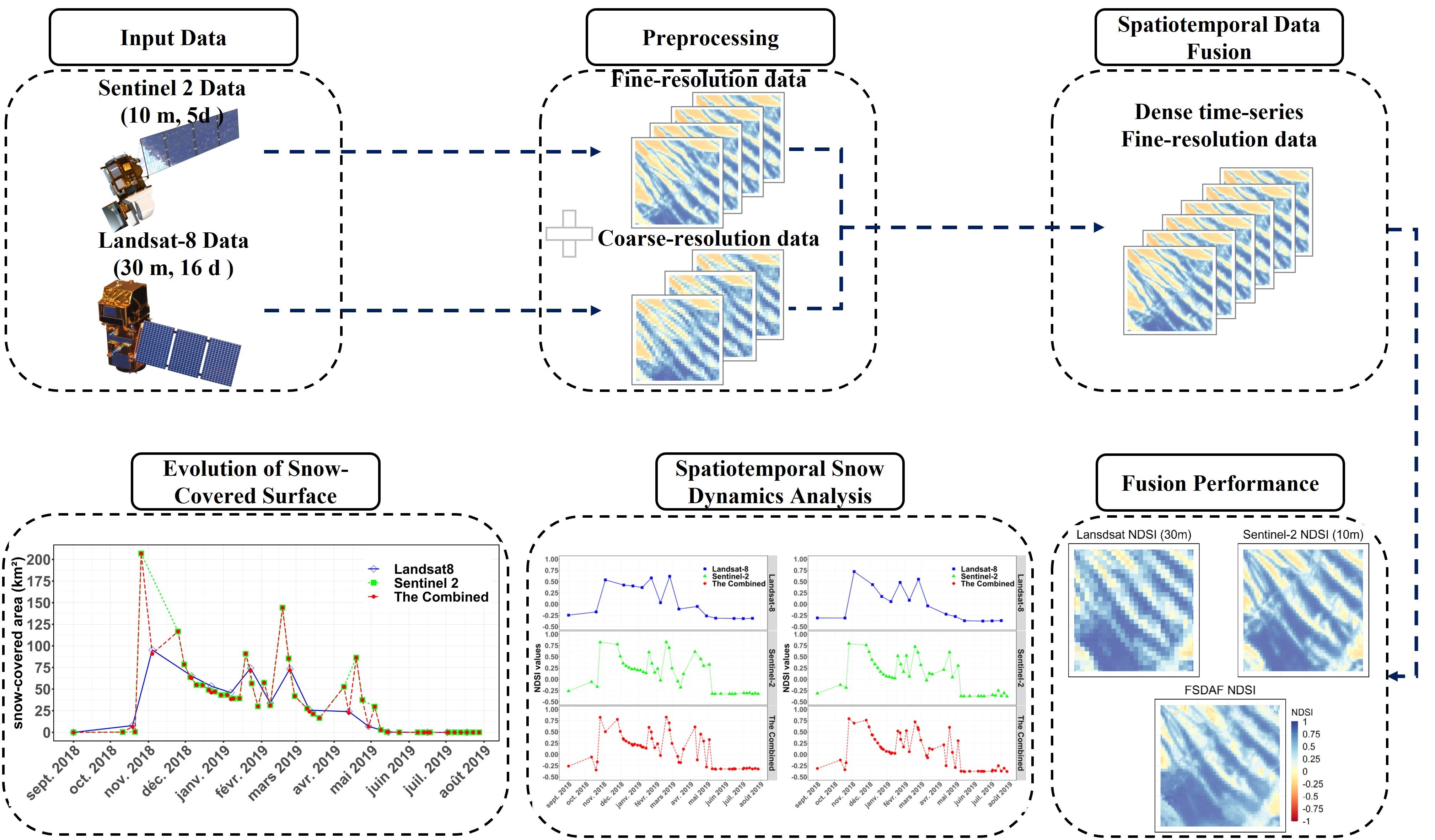
2.1. Study Area

The area of interest is in the center of Morocco; more precisely, in the High Atlas Mountains, whose culmination is the Toubkal, the highest peak in North Africa, at 4167 m. The High Atlas is a Moroccan mountain range oriented southwest/northeast; this chain belongs to the Atlas massif and, more precisely, to one of the three elements of the Moroccan Atlas, the other two being the Middle Atlas and the Anti-Atlas. The general morphology of the High Atlas is divided into three parts, the Eastern, Central, and Western High Atlas. The Atlas region includes important areas for Moroccan agriculture and many irrigated areas downstream. In general, the snow season falls during the winter months, and in the high-altitude areas extends for four to six months continuously from November to April [10,57].
The study area of interest consists of three large mountains, the Rat Mountain in the northwest with an altitude of 3781 m, the TigNousti Mountain in the southwest with an altitude of 3210 m, and the Tarkedid Mountain at 3565 m to the east of the study area (Figure 1).

2.2. Remotely Sensed Data Acquisition

The L8 OLI and S2 MSI images collected between 2015 and 2021 are the satellite data used in this research.
The L8 satellite was placed into orbit in February 2013, it observes the land cover with a revisit time of 16 days [58,59]. The Operational Land Imager (OLI) and the Thermal Infrared Sensor (TIRS) are instruments on board the L8 satellite. The OLI sensor for multispectral image acquisition in nine bands, with a spatial resolution of 30 m for 8 spectral bands and a spatial resolution of 15 m for the panchromatic band. In addition, the TIRS radiometer provides infrared data.
The Copernicus S2 mission is composed of a pair of two similar satellites called S2A and S2B, that offer high-resolution optical images with a high revisit capability from five to ten days using both satellites. However, not all images taken could be utilized due to the presence of massive cloud cover in the study area. The multispectral instrument (MSI) aboard S2 collects 13 overlapping spectrum bands at wavelengths from 0.4 to 2.2 μm: visible and near-infrared at 10-m spatial resolution, red edge and near-infrared at 20-m spatial resolution, and atmospheric bands at 60-m spatial resolution [60,61].
Data from L8 and S2 were downloaded using the USGS On-Demand Interface (ESPA) and the Theia Geographic Data Center, respectively. Previously, the L8 and S2 data were prepared and processed from atmospheric effects. In this study, it is important to note that only the cloud-free images of L8 and S2 were used to remove the effect of cloud contamination, therefore all the data we acquired does not have any cloud contamination in our selected test area.
In preparation of the following sections, where we will recapitulate the STF techniques, the primary step before implementing the fusion is the choosing of the set of L8 and S2 image pairs acquired on the same date that are used as inputs for the fusion models. After the choice of dates when S2 coincides with L8 over the study area from 2015 to 2021, we used the temporal profile of the average NDSI values evolution for each image of the S2 series to find out the specific dates when snow fell and select the cloud-free ones to obtain a chain of snowy and cloud-free L8 and S2 image pairs. Figure 2 shows the availability dates of the L8 and S2 image pairs, the type of utilization, and the average NDSI values for each acquisition date over the study area.

2.3. Estimation of Snow Surfaces from Satellite Images (Snow Cover Area)
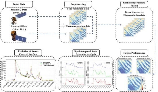
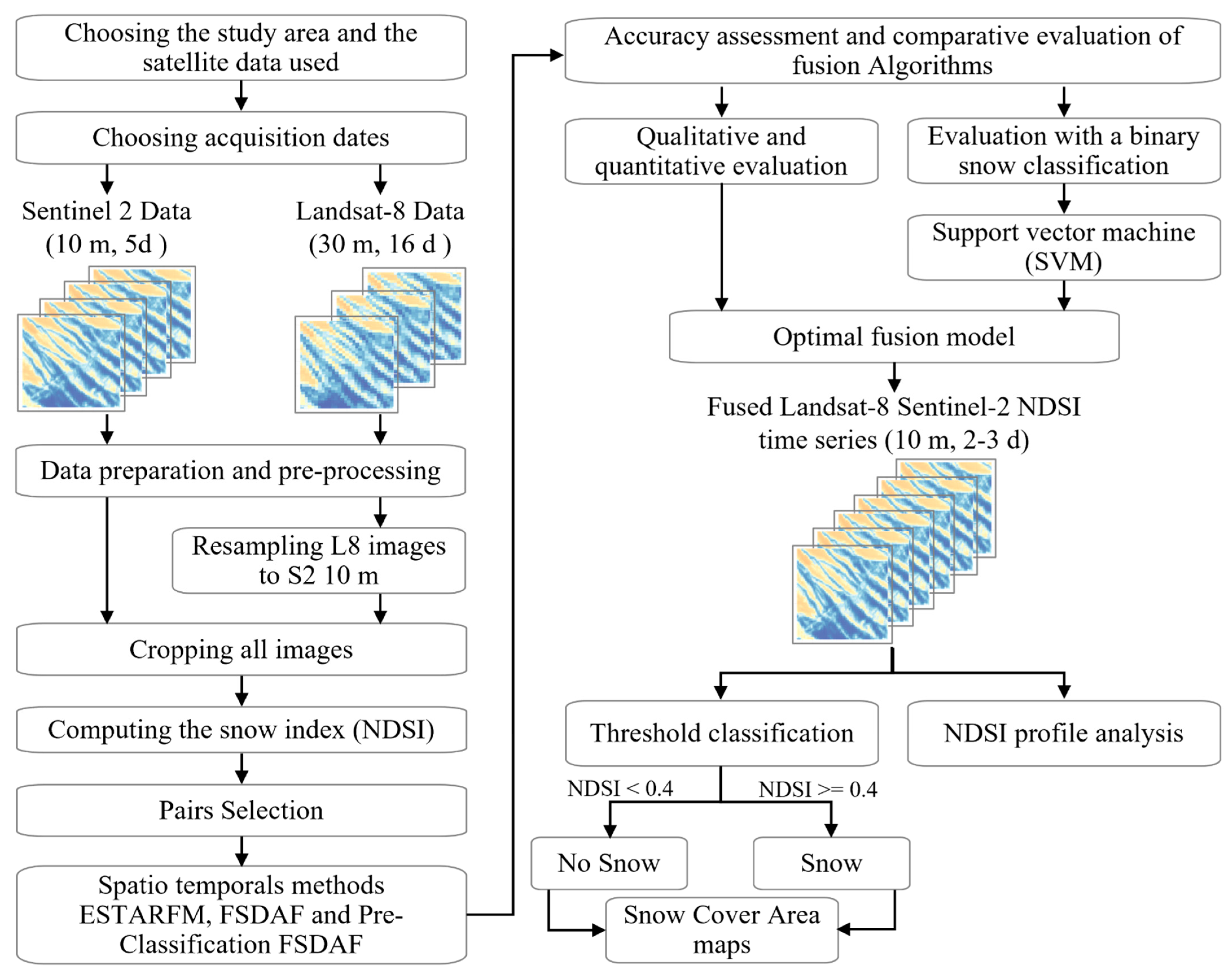
The reflectance of snow varies greatly with wavelength. The snow is characterized by low reflectance in the mid-infrared and high reflectance in the visible and near-infrared, which allows it to be distinguished from clouds, which are generally characterized by higher reflectance in both the mid-infrared and the visible [62,63]. Thus, with these optical properties, the identification of snow cover is relatively easy when the satellite image is multispectral or hyperspectral and contains bands in the visible and mid-infrared (MODIS, L8, S2).
The estimation of snow cover area using satellite data was achieved by computing the NDSI. The NDSI is derived from the contrast of the visible and the mid-infrared reflectance of the snow [64], which is the most widely used index for delineating the presence of snow or ice, as it is a normalized ratio of the difference in band reflectance that takes advantage of the unique signature and spectral difference to indicate the presence of snow relative to surrounding characteristics and even relative to clouds. The literature agrees that the green channel should be used, although the red channel may be suitable, and for the mid-infrared, the channel around 1.6 µm is most appropriate, as this is where the reflectance of snow is the lowest. The NDSI is defined by the following formula:
NDSI = ρ green     ρ swir ρ green +   ρ swir
where ρ green   and ρ swir are the visible and mid-infrared reflectance, respectively. In this context, to calculate the NDSI from L8 channels, we use the B3 (green) and B6 (SWIR) bands, and from S2 channels, we use the B3 (green) and B11 (SWIR) bands.
There is an agreement in the literature that the NDSI must be greater than 0.40 to be considered snow [22,64]. Generally, this value corresponds to a pixel covered by at least 50% of snow. This threshold can vary by ± 0.05 according to the time of the year, the type of snow, or the area considered. A pixel completely covered with snow will have an NDSI close to 1.

2.4. Methodology

Figure 3 illustrates the methodology used in this research. The multi-source remote sensing images were prepared based on their features and merged using STF techniques (ESTARFM, FSDAF, and pre-classification FSDAF) after choosing pairs of images that are used as input for these fusion models. Then, a qualitative and quantitative assessment of the fusion approaches was performed to determine the optimal fusion model that can be used to generate NDSI image series with both high spatial and temporal resolution. Lastly, the fused product NDSI values were used to construct snow cover area (SCA) maps based on snow index thresholding classification, as mentioned in the earlier section.

2.5. The Spatio-Temporal Data Fusion Method

In the past decades, many spatio-temporal image fusion approaches have been elaborated and used in the remote sensing domain. Although the main bases of spatio-temporal fusion approaches can differ significantly, the principal objective of each model is to combine fine spatial resolution satellite data but long revisit time with low spatial resolution satellite data but short revisit time at a reference date to generate image time series with fine spatial resolution and short revisit time [42].
The steps of these approaches are relatively similar. These models have a fundamental step of finding similar, homogeneous, and neighboring low-resolution pixels using a sliding window and assigning every comparable pixel a weight computed based on the spatial and spectral distance. The fine resolution pixel values of the similar, homogeneous, and neighboring pixels are used to determine the transformation coefficients and are then used to generate the fine resolution reflectance of each center pixel from the low-resolution image at the target fusion date. Among them, ESTARFM, FSDAF, and pre-classification FSDAF methods are three comparatively advanced approaches that have been selected and compared in this research to produce fused NDSI from L8 and S2 data.
There are several techniques to select similar, homogeneous, and neighboring pixels to the central pixel of the moving window. The ESTARFM approach provides two techniques to find similar pixels: The first one consists in applying an unsupervised clustering algorithm on the fine resolution image (NDSI S2) and the pixels that have the same land cover type and belong to the same group as the central pixel in the sliding window are identified as similar pixels. The second technique is based on the calculation of the reflectance difference between the central pixel and the neighboring pixels in the sliding window of the fine resolution image [47]. The pixels with a difference in reflectance lower than a threshold are considered as similar pixels. The threshold used is determined by the standard deviation of the pixels in the fine resolution image in the sliding window and the number of estimated classes in the image [24]. In addition, the FSDAF approach uses a strategy like ESTARFM for selecting pixels similar to a central pixel by choosing from the set of pixels in the sliding window the pixels with the smallest spectral difference in the same class as the central pixel [42].

2.5.1. The ESTARFM Method

The ESTARFM method was developed to enhance STF by exploiting correlation to merge multisource data and, at the same time, to produce precise results in the complicated and heterogeneous earth surface. To estimate a high-resolution image at a fusion date, the ESTARFM model requires a minimum of two fine- and coarse-resolution image pairs collected at two reference dates, in addition to a collection of coarse-resolution images for the fusion dates. Before applying the ESTARFM, each image should be preprocessed to obtain the georeferenced cover reflectance [47].
The implementation of the ESTARFM model consists of four main steps:
(1) First, two images with high resolution are employed to find similar pixels to the pixel located at the center of a moving window;
(2) Then, the weights of all comparable pixels (Wi) are computed according to the spectral similarity with the fine image (S2), the temporal distance to the reference pair, and the spatial distance to the adjacent pixels;
(3) Next, by integrating a linear regression method to similar pixels at low and high resolution, the conversion coefficients (Vi) are determined;
(4) Finally, the pixel weights (Wi) and conversion coefficients (Vi) are used to predict the high-resolution image at the fusion date.

2.5.2. The FSDAF Method

The second method used in this research is the FSDAF, considered one of the newest STF methods, which can work on difficult and sudden land cover changes, primarily due to its combined use of the advantages of both the interpolation method known as Thin Plate Spline and the spectral de-mixing analysis. The FSDAF method requires only a pair of low and high-resolution images at the reference date and a low-resolution image at the predicted date. Before executing the FSDAF model, the high- and low-resolution images must be co-registered and calibrated to the identical physical quantity [42]. The co-registration procedure can be summarized in these steps: (1) reprojection of the coordinates of the L8 image on the S2 image, (2) resampling of the L8 image to the S2 image using the nearest neighbor method, (3) georeferencing the L8 image onto the S2 image by choosing checkpoints or maxing out the correlation between both images, (4) then, the images are cropped to the same size [23].
Generally, the FSDAF method consists of six main steps:
(1) Classify the NDSI S2 image at time t1: In this model, an unsupervised classification algorithm i.e., ISODATA, is employed to classify the input high-resolution image to automate the FSDAF. We specify the maximum and the minimum number of classes used by the classification algorithm, which can be set based on previous knowledge of the region of interest or by a close visual examination of the high-resolution source image. ISODATA generates efficient classification results by fusing and dividing clusters based on the pixel value distribution in the characteristic space. The input fine resolution S2 image was classified into two classes: snow and non-snow, to obtain the fraction of snow in each coarse pixel of L8;
(2) Estimate the temporal variation of every cluster in the NDSI L8 from time t1 to time t2; the temporal change of a coarse pixel is the change in NDSI value between times t1 and t2. According to the spectral linear mixing theory, the temporal change is the weighted sum of the temporal change of all its component classes, it is defined as follows:
Δ C ( x i , y i ,   NDSI ) = c = 1 l f c ( x i , y i )     Δ F ( c ,   NDSI )
where ( x i , y i ) is the coordinate index of the ith pixel; C t 1 ( x i , y i ,   NDSI ) and C t 2 ( x i , y i ,   NDSI ) are the NDSI values of the coarse pixel (e.g., L8) at position ( x i , y i ) at time t1 and t2 respectively; Δ C ( x i , y i ,   NDSI ) is the change in NDSI value of the coarse pixel ( x i , y i ) between time t1 and t2; f c ( x i , y i )   is the fraction of the class c of the coarse pixel (xi, yi); Δ F ( c ,   NDSI ) is the change of the NDSI value of the fine resolution class c between time t1 and t2.
(3) Use the temporal variation at the class level to predict the NDSI L8 image at time t2 and compute the residuals at every coarse pixel; the prediction of the fine pixel values at time t2 is determined by adding the temporal change to the fine pixel values observed at time t1:
F 2 TP ( x ij , y ij ,   NDSI ) = F 1 ( x ij , y ij ,   NDSI ) + Δ F ( c ,   NDSI )
where F 2 TP ( x ij , y ij ,   NDSI ) is the temporal prediction that uses only the information of temporal change between t1 and t2; Δ F ( c ,   NDSI ) is the change of the NDSI value of the fine resolution class c between time t1 and t2; F 1 ( x ij , y ij ,   NDSI )   and F 2 ( x ij , y ij ,   NDSI ) are the NDSI values of the j-th fine pixel (e.g., S2) in the coarse pixel at the position ( x i , y i ) at time t1 and t2 respectively.
The temporal prediction of the high-resolution image at time t2 is already determined, but it is not a good prediction when there is a major change in land cover type between t1 and t2. Furthermore, a residual between the actual values and the temporal prediction of fine pixels was introduced by Zhu et al. [42]. The distribution of the residual R ( x i , y i ,   NDSI ) at the fine pixels of a coarse pixel is defined by the following equation:
R ( x i , y i ,   NDSI ) = Δ C ( x i , y i ,   NDSI ) 1 m [ j = 1 m F 2 TP ( x ij , y ij ,   NDSI ) j = 1 m F 1 ( x ij , y ij ,   NDSI ) ]  
where m is the number of fine pixels in a coarse pixel
(4) Estimate the NDSI S2 image from the NDSI L8 image at t2 with a thin plate spline (TPS) interpolator which is a technique based on splines and spatial dependence for interpolation and smoothing of point data in order to guide the residual distribution;
(5) Using a weighted function to distribute the temporal predictive remainders according to the geographical homogeneity and the TPS prediction;
(6) Get the result of the NDSI S2 prediction using the neighborhood information.

2.5.3. The Pre-Classification FSDAF Method

The pre-classification FSDAF method has the same algorithm and steps as the FSDAF method, and the only difference is that instead of using the simple classifier-unsupervised classification (ISODATA) embedded in FSDAF, the pre-classification model uses a supervised SVM (support vector machines) classifier to classify the image at high resolution, which is the first step in the model.
The support vector machine (SVM) is a supervised statistical nonparametric machine learning technique that performs well in classifying complicated data. The approach is introduced in its original formulation using a set of tagged data items, and the learning SVM approach focuses on finding a hyperplane that splits the data set into several predefined classes in a way that is coherent with the learning items [65]. According to the literature, SVMs often generate higher classification accuracy than conventional approaches because of their capability to handle successfully smaller learning data sets [66]. On the other hand, comparative research has examined their performance with other feature classifiers for different types of landscape cover. For example, Huang et al. [67] found that SVM significantly surpassed decision tree (DT) or maximum likelihood (MLC) regarding the accuracy of the classification and outperformed even the multilayer perceptron neural networks (MLP). Su et al. [68] applied both the MLC and the SVM on an image from the Multi-angle Imaging SpectroRadiometer to distinguish different types of vegetation and they noticed that the SVM surpassed the MLC significantly. In addition, the advantages of SVM are better classification accuracy compared to traditional parametric classifiers such as unsupervised k-means clustering [69].
In our case, the idea of the SVM classifier is to classify the input S2 image into two classes: snow and non-snow. The result of this classification will be used as input for the pre-classification FSDAF model in order to consider snow and non-snow pixels during the model training. The implementation of the SVM classifier is realized on the ENVI software which facilitates the use and parameterization of the model, for example the kernel function and two parameters C and gamma which must be determined for the model configuration. The Gamma and penalty (C parameter) are important parameters that affect the accuracy of the SVM classification. In this case, RBF kernel function is selected, and the combination of (Penalty = 100, gamma = 0.167) is chosen.

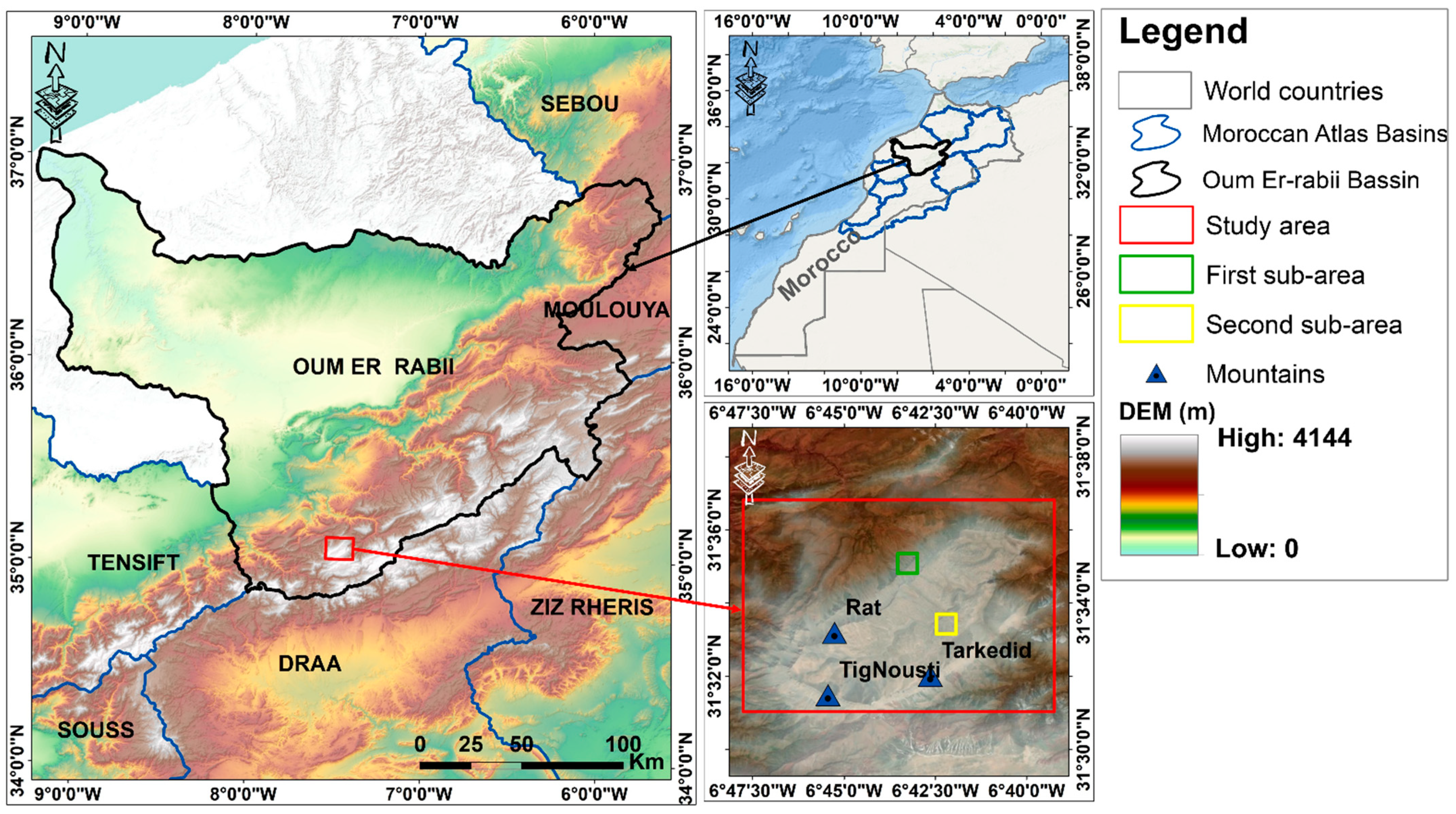
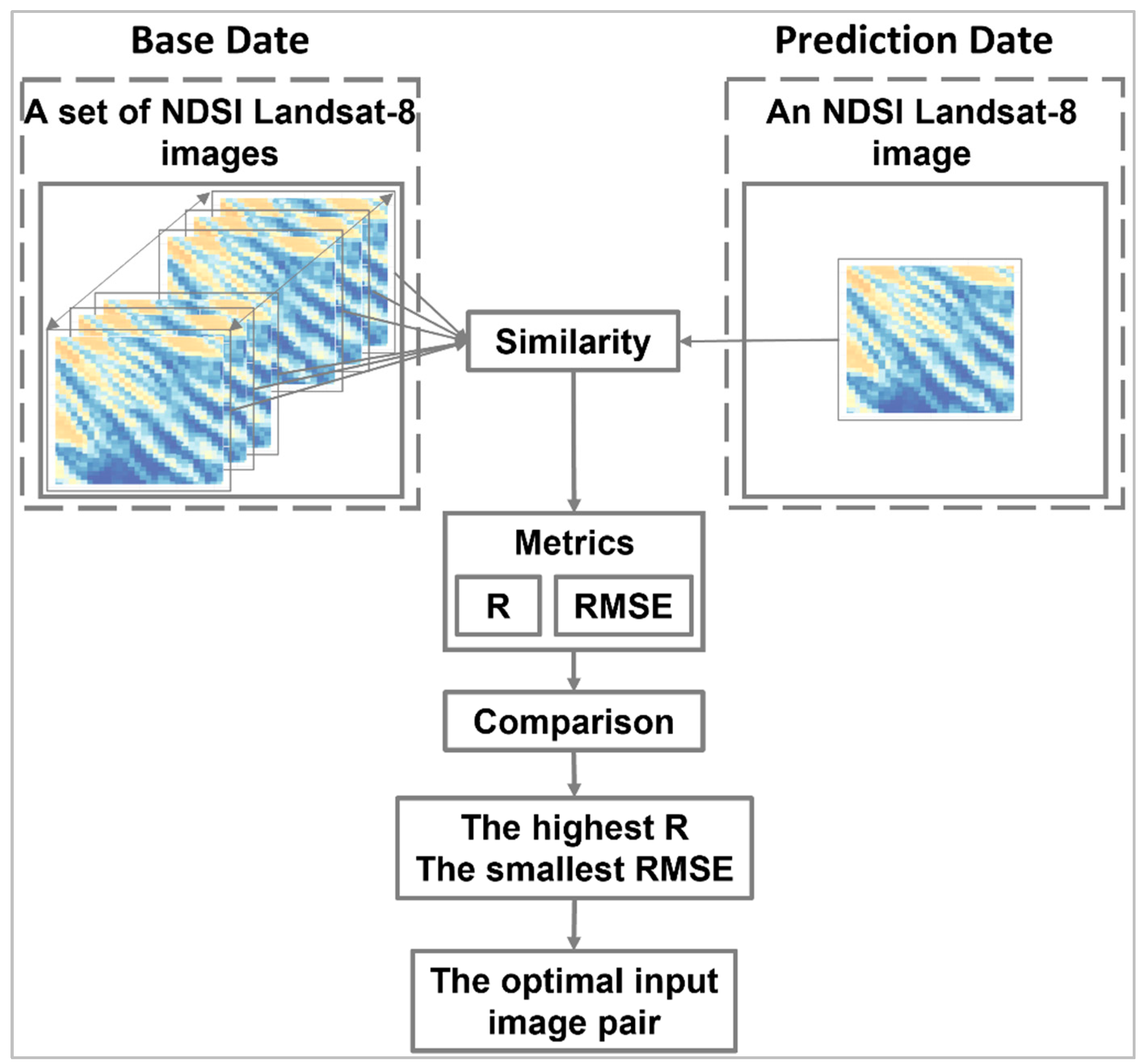
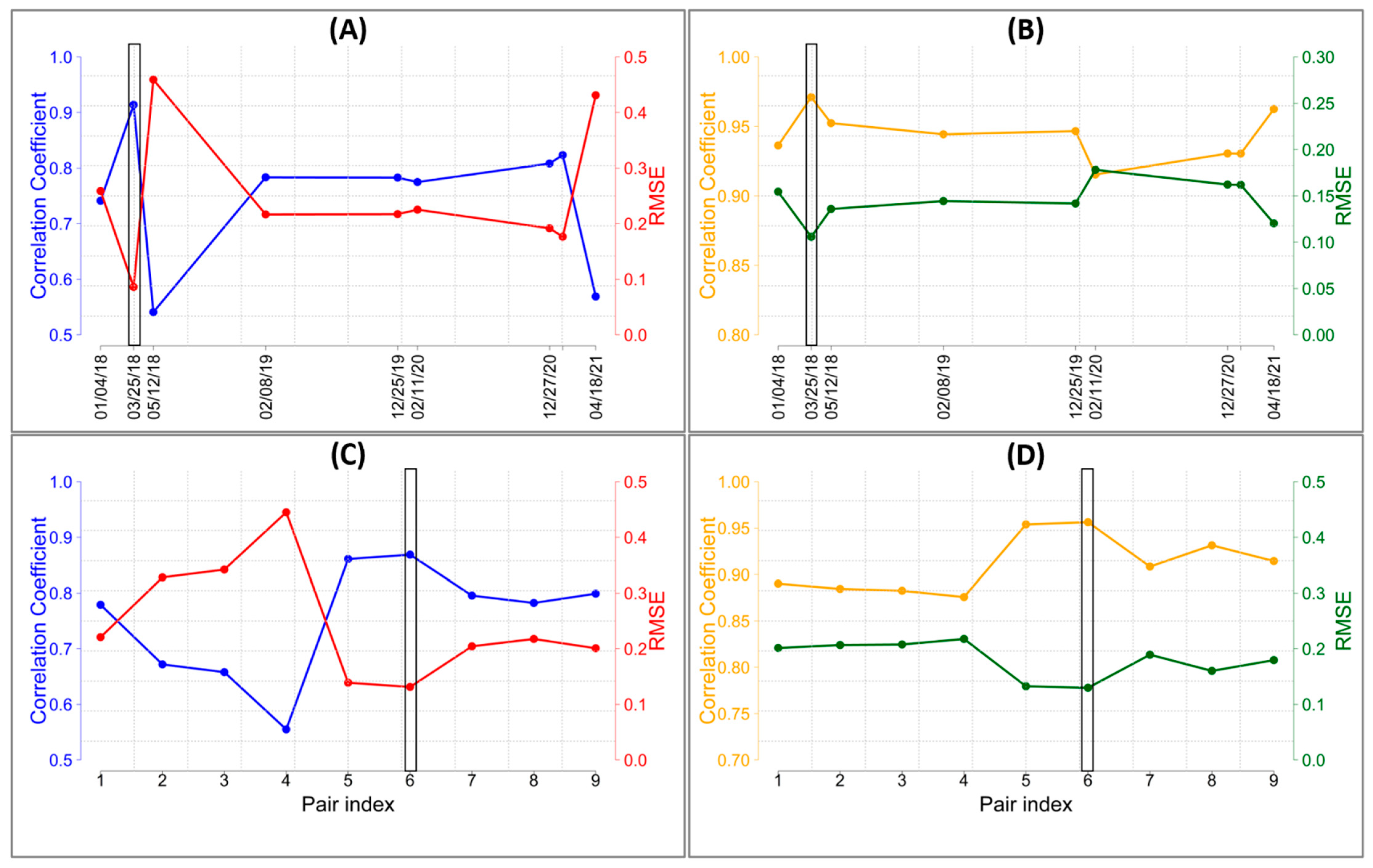
2.6. Selection of Optimum Input Image Pairs

The choice of optimum input image pairs for STF techniques is a critical step before their implementation which improves the prediction accuracy. Recently, there has been no existing method to automatically determine these image pairs. In our case, we proposed an approach that considers both the similarity criterion and the error quantification criterion between the low-resolution image at the reference date and the one at the merge date.
According to which the optimal input pair for fusion is the one that has the highest correlation coefficient with the smallest error with the low-resolution image at the desired prediction date (Figure 4). The correlation coefficient ( corr ( ρ pi ) ) and the error ( RMSE ( ρ pi ) ) between the L8 image at the prediction date ρ p and the one at another date ρ i are measured in order to evaluate the similarity and the difference between the two L8 images. These two indices are calculated according to Equations (5) and (6) respectively,
corr ( ρ pi ) = j = 1 N ( ρ p ( j ) m ρ p ) ( ρ i ( j ) m ρ i ) Std ρ p Std ρ I
RMSE ( ρ pi ) = j = 1 N ( ρ p ( j ) ρ i ( j ) ) ² N
where the N represents the number of L8 image pixels. The ρ p ( j ) and ρ i ( j ) represent the NDSI value of the j-th pixel in the NDSI L8 image at the prediction date and that at another date, respectively; m ρ p and m ρ i are the average of the values of ρ p and ρ i , respectively.
For this work, we proposed to predict the image of the date 4 April 2016. Furthermore, to evaluate the performance of the fusion models according to the image pairs used, the different input image pairs were considered, as shown in Table 1.

2.7. Quantitative and Qualitative Evaluation of Fusion Techniques

The STF findings were qualitatively and quantitatively compared to the real image of S2 from 4 April 2016, from the prediction date to verify the accuracy of the fused NDSI and synthesize their performance variances.
The qualitative evaluation is based on a visual examination of the real and predicted NDSI. On the other hand, as a proxy for quantitative evaluation, correlation coefficient (R), root-mean-square error (RMSE), coefficient of determination (R²), and the average absolute difference (AAD) were used to compare the prediction performance in STF algorithms.
The correlation coefficient measures the strong relationship between a merged image A (estimated NDSI) and its associated base image B (actual NDSI S2). R may be computed using the formula:
R ( A , B ) = i = 1 N ( A i m A ) ( B i m B ) Std A Std B
where A i   and   B i   are the NDSI value of the i-th pixel in A and B, respectively; m A and m B are the average of the values of A and B, respectively; Std A ,   and   Std B are the standard deviations of A and B, respectively. The ideal value is 1, while the interval is between −1 and 1.
The coefficient of determination (usually referred to as R²) is a concept in the analysis of variance and regression analysis. It is a measure of the proportion of explained variance present in the data. Therefore, a higher R² value means that the model better describes the data. When the data consist of values y1, …, yn of a response variable and a model with predictor variables is applied to the data, then R2 is defined as follows:
R 2 = i = 1 N ( Y i Y ^ i ) ² i = 1 N ( Y i Y ¯ i ) ²
where Y ¯ i denotes the mean of the observations and Y ^ the prediction of Y i using the adjusted model.
The RMSE was used to compare the size of the error and gives an overall representation of the deviation between the merged NDSI image and its actual NDSI at a similar date. It is calculated by the following formula:
RMSE = i = 1 N ( A i B i ) ² N
where N represents the total number of pixels, and A i and B i   represent the NDSI value of the i-th pixel in both the estimated and observed images, respectively. The lower the RMSE value, the higher the model efficiency, and conversely.
The AAD was employed to denote the global merged NDSI image bias, and it is given as below:
AAD = i = 1 N | X i Y i | N
The smaller the AAD value, the smaller the predicted image bias, and conversely.

3. Results

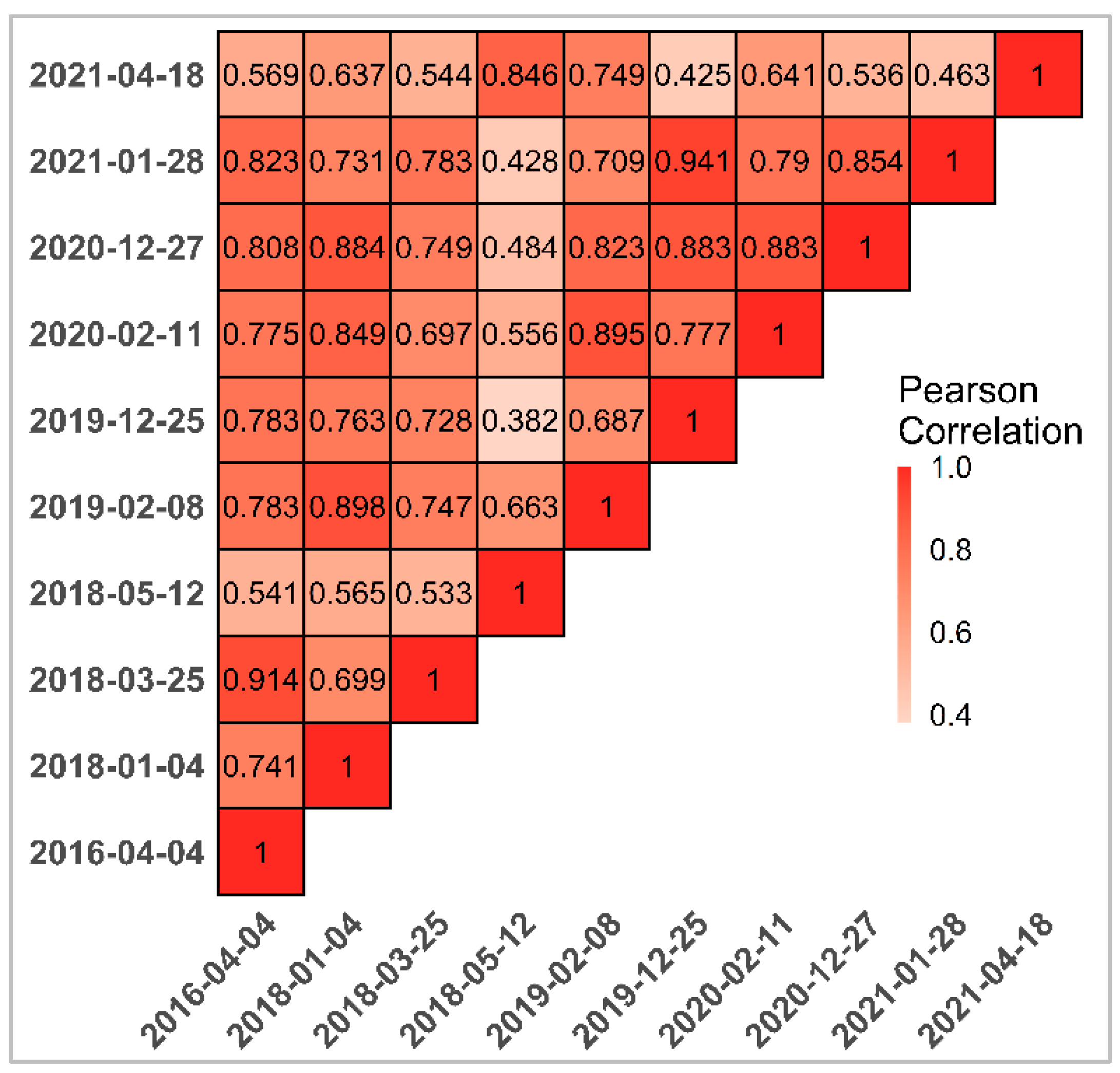
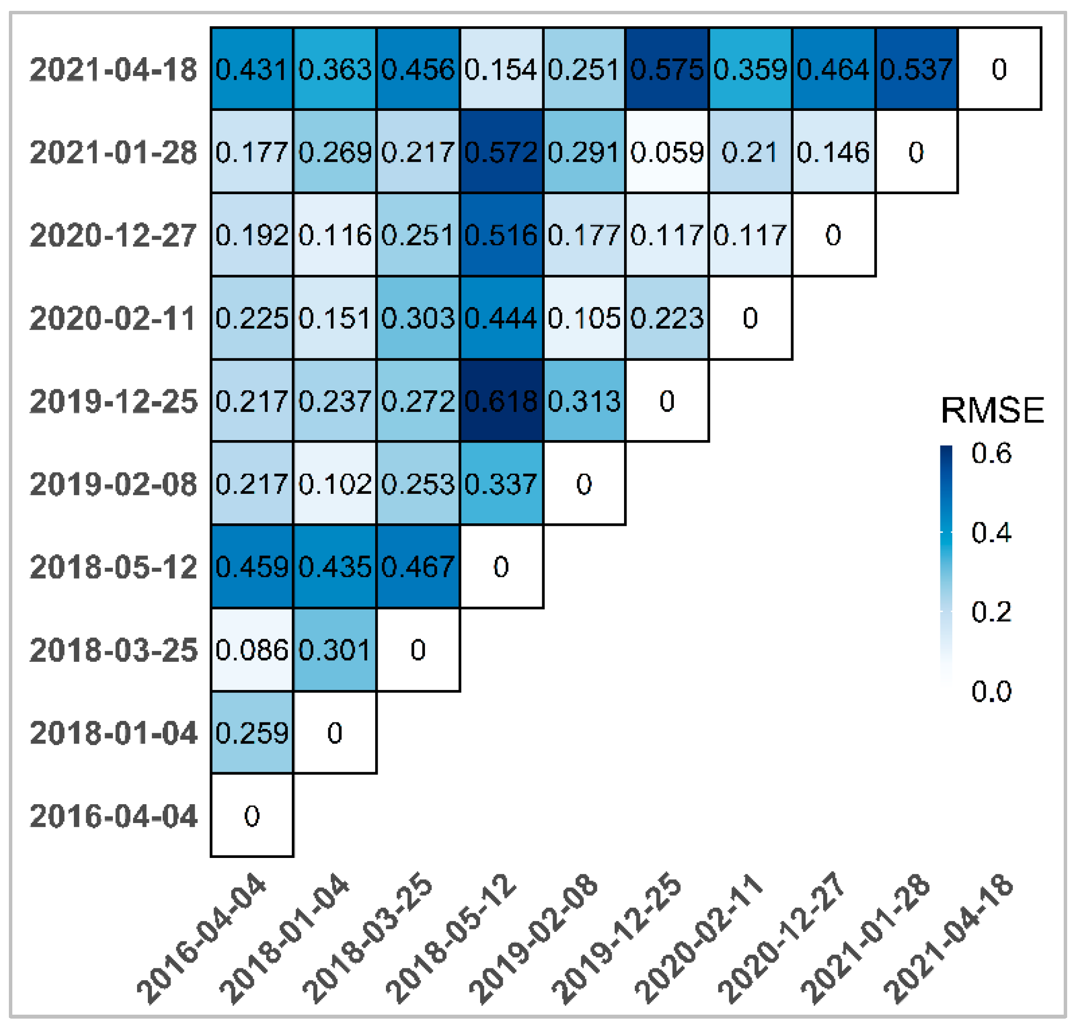
3.1. The Optimal Input Image Pairs

Among the image pairs mentioned in Table 1, we choose the optimal input image pairs for each STF model, as shown in Figure 5 and Figure 6, which represents the correlation coefficient (Figure 5) and the RMSE (Figure 6), between the total of pairs image covering the study area. These results give us an idea about the choice of the optimal image pairs, and as we chose previously to predict the image of the date 4 April 2016, we can see that the two pairs of 25 March 2018, and 28 January 2021, have the smallest error ( RMSE = 0.086 and RMSE = 0.177 respectively) and the largest correlation coefficients (R = 0.91 and R = 0.82 respectively) which allow us to use them for the spatiotemporal fusion models. Since the FSDAF algorithm requires only one image pair as input (L8 and S2), we use the 25 March 2018, image pair, which has the higher correlation coefficient and similarity index. In contrast, the ESTARFM algorithm requires two pairs of input images; for this reason, we use the two selected image pairs.
To validate the choice of the optimal input image pairs, we applied the FSDAF and ESTARFM models to estimate the high-resolution image corresponding to the chosen date using the different input pairs mentioned in Table 1. Different predicted images obtained for the same prediction date were evaluated using different statistical indices (e.g., correlation coefficient and RMSE) to confirm the choice of the optimal pairs as well as to evaluate the prediction performance using the other pairs.
Figure 7A,C present the correlation coefficients (red line) and the RMSE (blue line) between the NDSI L8 image at the prediction date and the other input image pairs at different dates for the FSDAF and ESTARFM models, respectively. Figure 7B,D present Correlation coefficient (orange line) and RMSE (green line) between the original NDSI S2 image at the prediction date and the other predicted images using different pairs as input images for the FSDAF and ESTARFM models, respectively.
We note that the L8 image predicted using the 23 March 2018 image pair previously identified as the optimal input for the FSDAF model (the second pair listed in Table 1 for FSDAF) has the highest correlation coefficient (R = 0.97) and lowest RMSE (RMSE = 0.10) with the actual S2 image compared to the other predicted images. Similarly, for the ESTAFM algorithm, the two image pairs previously selected as optimal (the sixth pair listed in Table 1 for ESTARFM) can estimate the L8 image at the desired prediction date with the highest correlation coefficient (R = 0.95) and lowest RMSE (RMSE = 0.12) with the real image, as indicated by the rectangles in Figure 7.

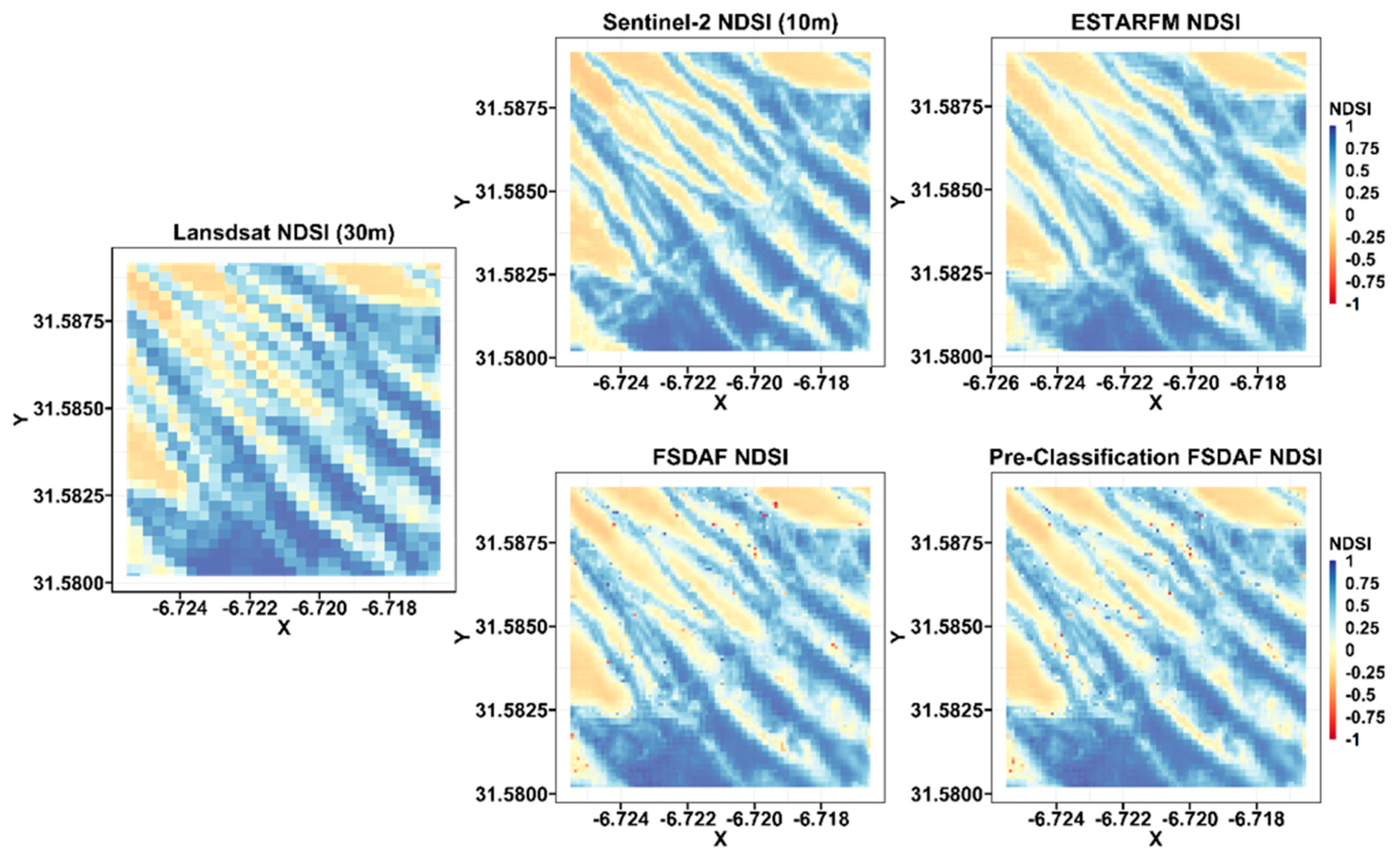
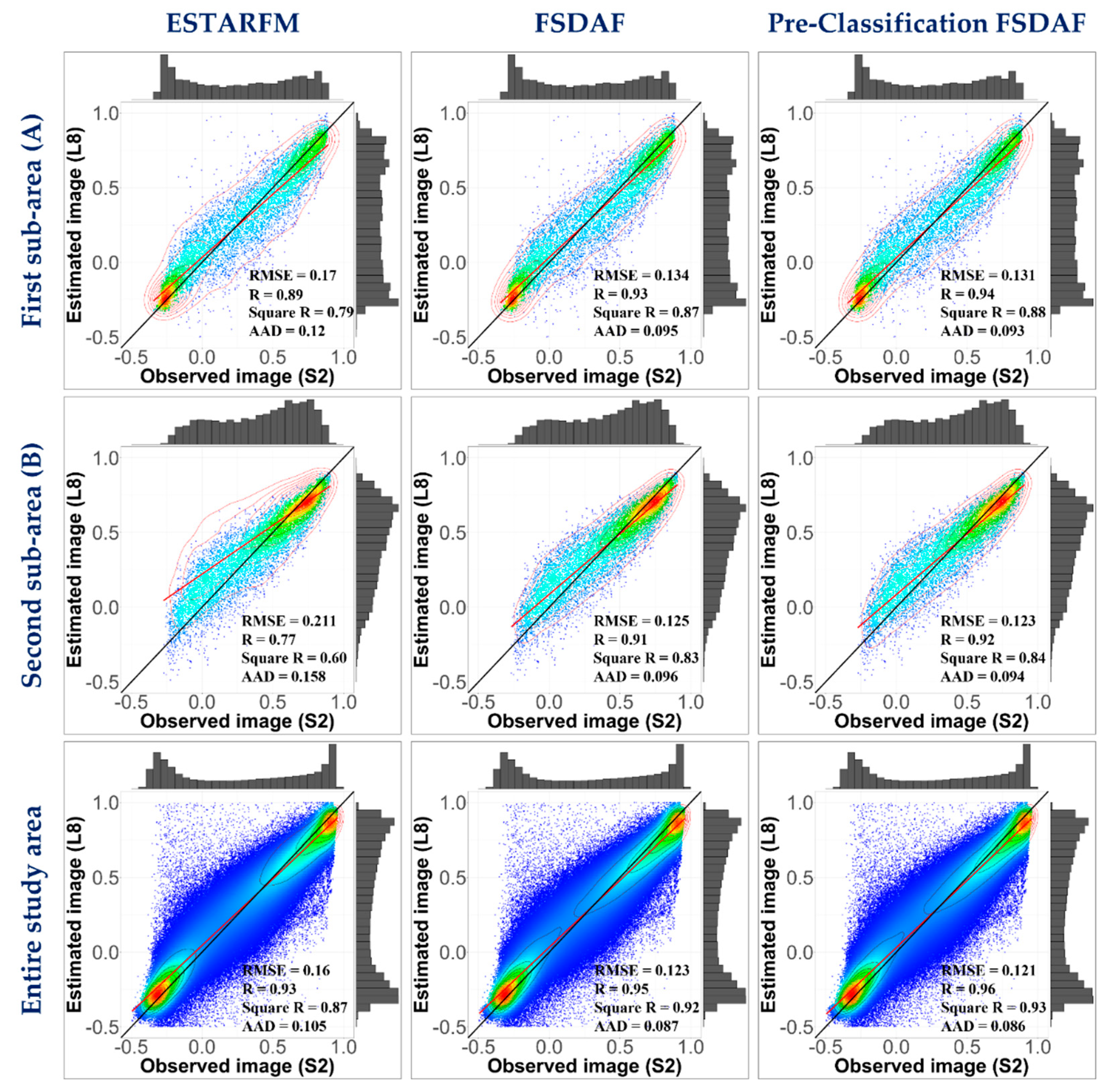
3.2. Fusion Performance

Figure 8 and Figure 9 provide a visual comparison of the synthetic NDSI (at 10 m) obtained by the different STF methods used (ESTARFM, FSDAF, and pre-classification FSDAF) with the real NDSI S2 (at 10 m) and the actual NDSI S2 (at 30 m) of the 4 April 2016, image for the two subareas A and B.
Visually, the images predicted by the spatio-temporal fusion approaches are typically similar to the real S2 image, which suggests that all models are capable of capturing spatial and temporal changes in both snow and snow-free areas, giving good accuracy for downscaling NDSI L8 images to a greater spatial resolution similar to NDSI S2 images.
Further analysis indicates that the predicted images by the pre-classification FSDAF and the FSDAF methods appear to be similar to the real NDSI image, slightly better than the one obtained with ESTARFM. This may be illustrated by the gradient color over the entire region studied as well as in the two sub-areas shown in Figure 8 and Figure 9. Though these prediction results may be fallacious or indirect, they merit a more thorough quantitative analysis for this reason.
In order to further investigate the differences between the predicted NDSI images from the three fusion models, we used the two previously mentioned sub-areas as an illustration, as shown in Figure 10. This figure shows the difference between the actual NDSI image, and the images predicted by the fusion models used ESTAFM, FSDAF, and pre-classification FSDAF. We have observed that the predicted NDSI image by ESTARFM presents more difference with the real NDSI S2 image than the other two models. Although the pre-classification FSDAF method presents slightly smaller differences than the FSDAF method as shown in Figure 10 for both sub-areas. To further this visual comparison, we quantified the differences between the images based on calculating the unaltered area between the actual and predicted images for the two sub-areas as shown in Table 2. The unaltered area refers to the total area where the actual NDSI S2 image and the estimated NDSI image took the exact same values. For example, for the entire study area, the pre-classification FSDAF model generates 94.10% of the surface area that has the same values as the actual NDSI S2 image, compared to 93.28% and 89.03% for the FSDAF and ESTARFM models, respectively. The same improvement can be seen for the pre-classification model for both sub-areas. The results indicate that the pre-classification FSDAF model can generally predict high-resolution NDSI images that most closely match the actual NDSI image by keeping the largest area with the same NDSI values compared to the other methods.
A further comparison between the three models used in this study is to compare the amount of snow estimated from the actual S2 NDSI and the predicted NDSI from the three fusion models. As shown in Table 3, the snow cover estimated from the pre-classification FSDAF model underestimates the actual snow cover by −0.25 km². On the other hand, there is an underestimation of −1.28 km² by the FSDAF model and an overestimation of 2.2 km² by the ESTARFM model in the snow cover estimation. This suggests that the pre-classification FSDAF model can estimate snow cover with less bias compared to the actual estimated amount of snow.
In this respect of the quantitative evaluation, Figure 11 shows the quantitative metrics, and the scatter plots of the NDSI predicted by the fusion models compared to the actual S2 NDSI acquired on 4 April 2016. The scatterplots fully confirmed the previous qualitative comparison observations. The scatter plots of the density for the three fusion models show a high correlation, indicating that all three methods can give an excellent estimate for a coarse-resolution image for the desired fusion date, but there are also notable differences in the prediction quality between the methods used.
As illustrated in Figure 11, there are fewer outliers in the pre-classification FSDAF model than in the other two models, FSDAF and ESTARFM, whose density scatterplots show a less dense and finer distribution over all snow and snow-free areas. In particular, for the snow-covered areas with the highest NDSI values, the pre-classification FSDAF model performs better than FSDAF and ESTARFM, as shown in the scatter plots for both subareas A and B. A similar pattern can occur with medium and low NDSI values, as can be seen in the scatterplots for all areas. In contrast, ESTARFM, FSDAF, and pre-classification FSDAF have similar abilities to predict NDSI values in both snow and snow-free areas.
Consequently, we quantified their performance by a quantitative comparison using various statistical indicators. From these measures, it appears that the FSDAF performed worse than the pre-classification FSDAF but better than the ESTARFM. In addition, pre-classification FSDAF generated the lowest RMSE and AAD (RMSE = 0.12 and AAD = 0.08) and the highest R and R² coefficients across all study areas (R = 0.96 and R² = 0.93) compared to the two other approaches.
Given the above aspects and the slightly better performance of the pre-classification FSDAF than FSDAF and ESTARFM, we chose it as the primary fusion model to predict and merge the entire L8 time series in our study area.

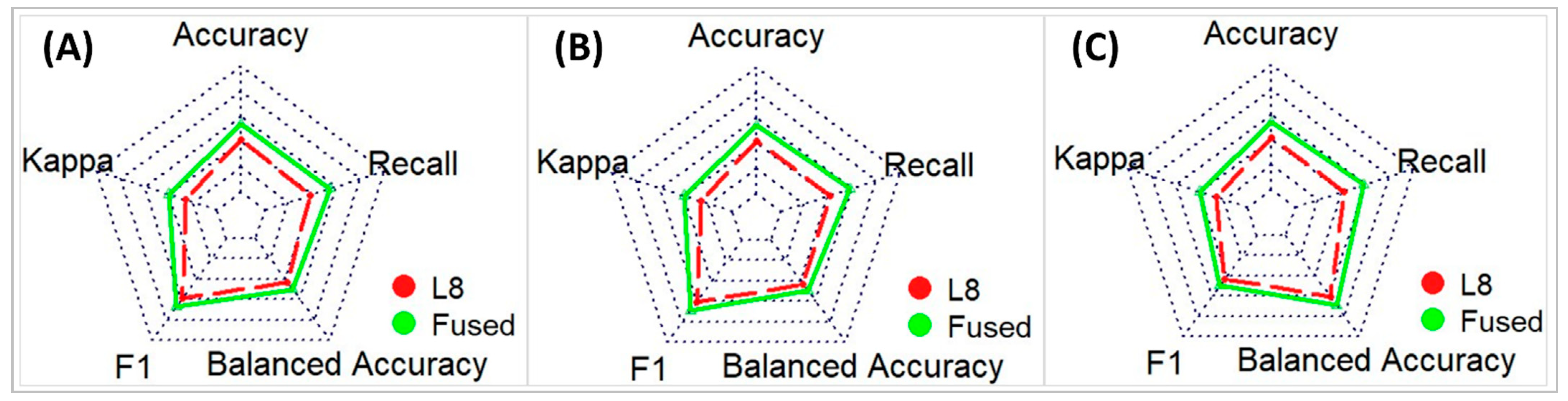
3.3. Assessing the Fusion Performance Using a Snow Binary Classification

The classification map of the high-resolution image (10 m resolution) of 4 April 2016, predicted by the pre-classification FSDAF model, with the classification map of the L8 image at 30 m obtained by applying different thresholds of NDSI snow indices (0.3, 0.35 and 0.4) were compared to the reference classification map.
Several skill scores such as “Accuracy”, “Cohen’s Kappa”, “F1-Score”, “Balanced Accuracy”, and “Recall” are used to evaluate these classification maps against the reference one (Figure 12).
A comparison of the snow cover areas obtained from different classification maps is essential to determine the ability and performance of the STF to estimate the snow cover, which was not accurately achievable using low-resolution data. As shown in Figure 12, with the downscaling NDSI images using the pre-classification FSDAF fusion model, the classification accuracy of the snow cover areas gradually improved.
In addition, the fused images with high spatial resolution provide precise quantification of the snow cover area in the mountainous regions. As shown in Figure 13, the estimated snow cover from the fused image is closer to that estimated from the reference image than that estimated from L8 for the different NDSI thresholds. This demonstrates that spatial resolution is a critical factor for accurate snow cover estimation, as already shown in previous works [25,26,27] that low spatial resolution is not sufficient to accurately estimate and capture snow evolution at both spatial and temporal scales. For this reason, we use the STF as a powerful tool to produce high spatial and temporal resolution images.

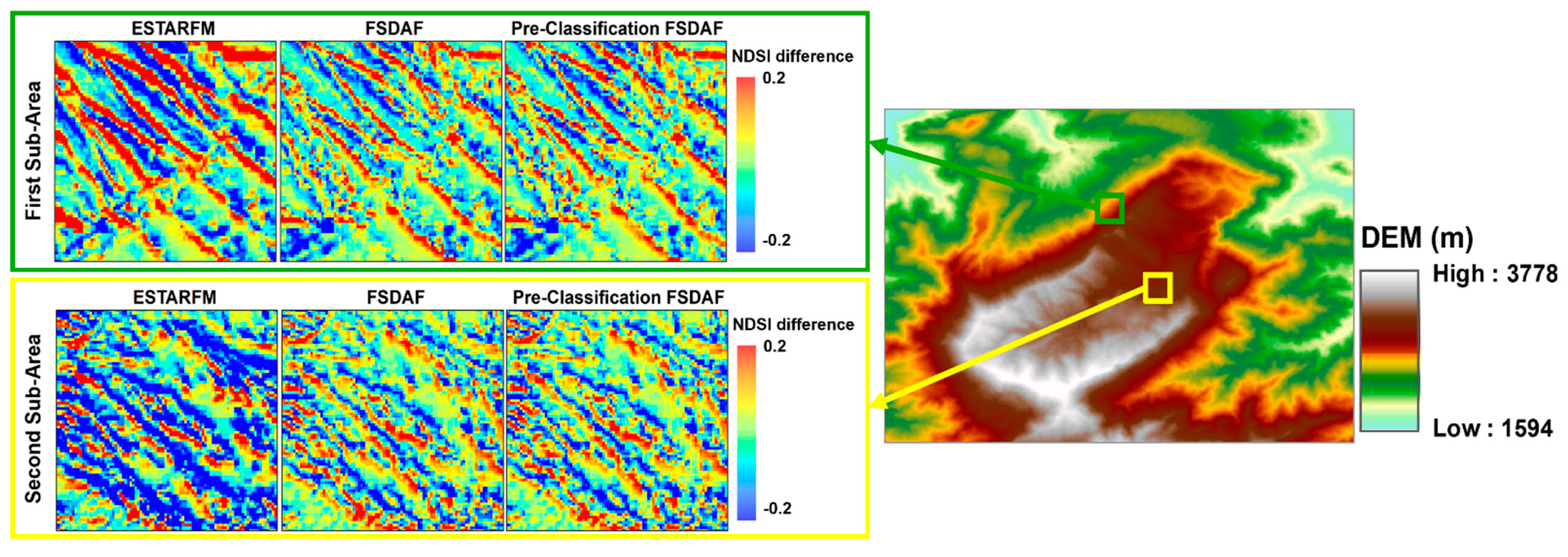
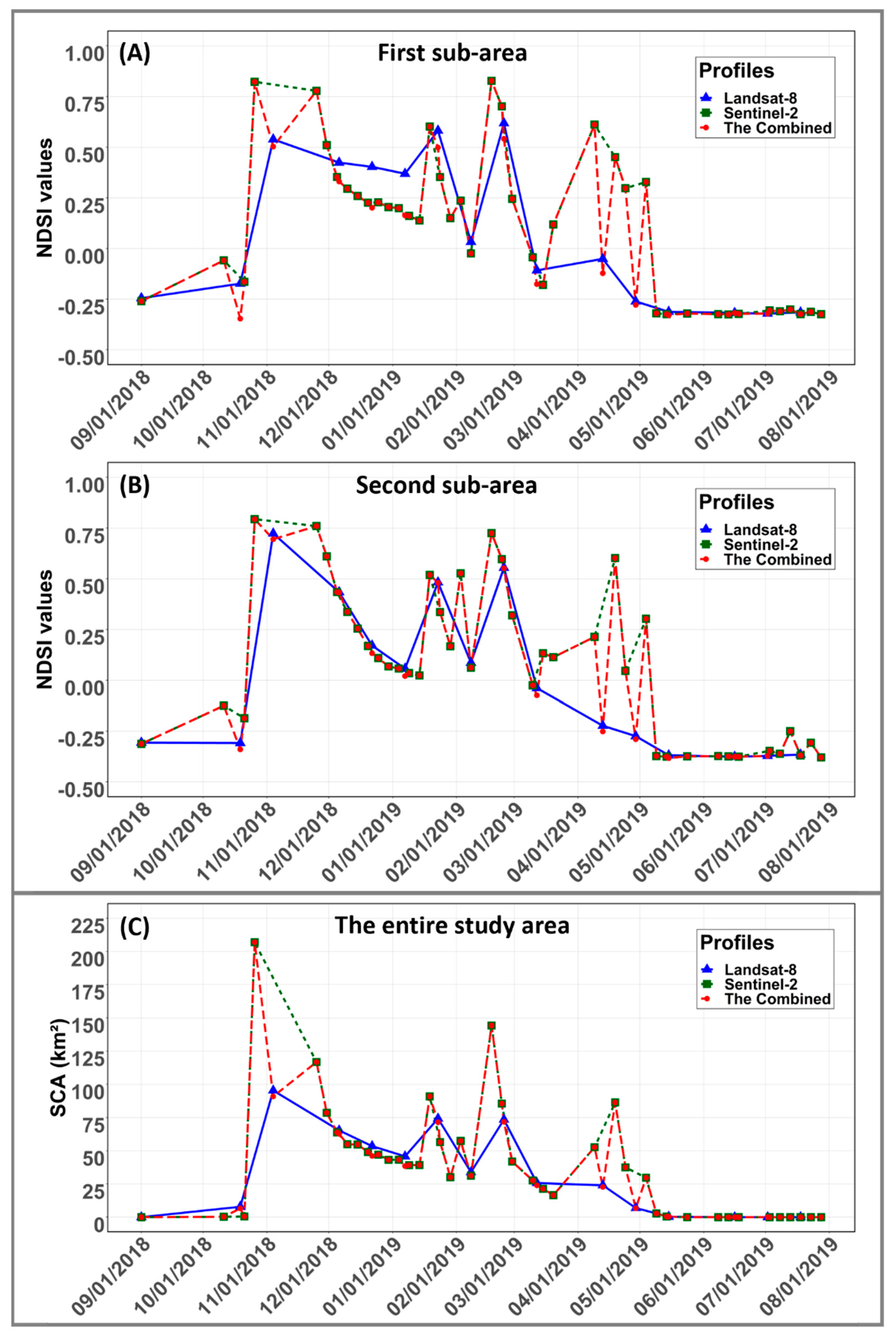
3.4. Analysis of NDSI Profiles

Based on the application of the pre-classification FSDAF fusion model, each of the L8 NDSI time series images with a spatial resolution of 30 m and a revisit time of 16 days was enhanced in terms of its spatial resolution to generate an NDSI time series with the same resolution as S2 (10 m). This merged time series was combined with existing S2 NDSI observations to increase the number of accurate NDSI images with a finer time step.
The panels A and B in Figure 14 represent a comparison of different time-series profiles of NDSI obtained from L8 (blue line) and S2 (green line) satellite data and their combined use by the pre-classification FSDAF STF method (red line) and during the 2018/2019 hydrological year using the NDSI average for both sub-areas A and B.
In general, the fused NDSI profiles show a clearly defined and unique characteristic of the snow cover in the mountainous regions. It is evident from the visual examination of the panels A and B in Figure 14 that the fusion of the S2 and L8 allowed for continuous monitoring of snow cover changes over the water year and helped to capture precise temporal variations while maintaining high spatial resolution, which was not achievable previously using only the S2 or L8 data. In particular, in some semi-arid regions (e.g., the first sub-area and second sub-area shown in Figure 14) characterized by high snow variability, the snowfall cycles were better visualized in the merged NDSI time series than in the individual L8 or S2 series as illustrated by the red profiles. In addition, some abrupt snow events (e.g., rapid melt or snowfall) cannot be captured more accurately using only the individual time series (L8 or S2). Therefore, an event that appears in one product is not captured in the other. However, the merged NDSI L8/S2 time series captures all events that occurred during the water year.
These results, combined with earlier conclusions on the evaluation of the quality and coherence of the estimated NDSI, suggest that our STF model is adapted for the construction of image time series for continuous snow cover monitoring in mountainous areas characterized by rapid snow surface dynamics.

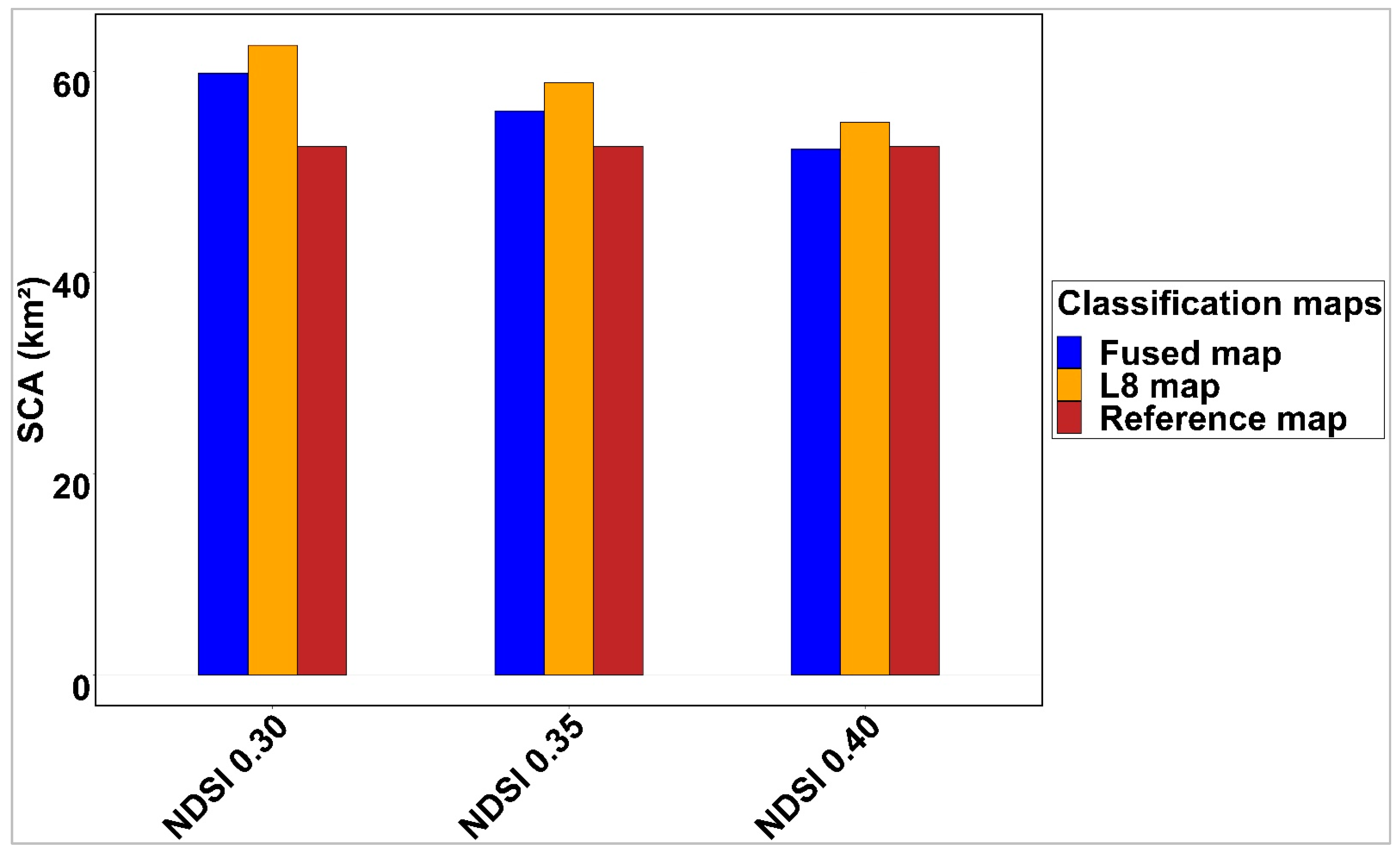
3.5. Spatio-Temporal Fusion Effect on Snow Cover Area Extraction

After generating dense NDSI image time series with 10 m spatial resolution, covering the 2018/2019 hydrological year (between 1 September 2018, and 28 July 2019), the snow surface maps (snow/no snow) were developed as the first requested products, and these maps are derived from the NDSI by thresholding. As mentioned in Section 2.3, the literature agrees that the NDSI must be greater than 0.40 to be classified as snow, so this threshold was used to classify the NDSI into two classes: snow and snow-free to obtain snow-covered area maps.
The panel C in Figure 14 shows the comparison between different profiles of snow surface evolution derived from L8 and S2 data and their fusion in the study area during the hydrological year 2018/2019 (in blue L8, in green S2, and in red their combination). This figure illustrates the impact of multisource data fusion on the accurate monitoring and estimation of the snow-covered area in mountain regions.
The merged product (red line) has provided unique advantages for snow cover monitoring that allows for the identification of missed snow events by using a single product. However, in terms of snow area estimate, the fused series of L8 and S2 data with a high spatial resolution (10 m) provides an accurate estimation of the snow surface for each map during the hydrological year (SCA (Combined) = 2091.82 km²) which cannot be properly assessed using only the time series of L8 (SCA (L8) = 506.35 km²) or S2 (SCA (S2) = 1650.10 km²). Moreover, the amount of snow obtained from a 30 m resolution image (pixels of 900 m²) does not have the same accuracy as that from a 10 m resolution image (pixels of 100 m²). These results show the impact of fusion in terms of improving the image spatial details and increasing the number of observations.

4. Discussion

This research illustrates that the combined use of next-generation multispectral sensor data from the L8 and S2 satellites can improve snow cover mapping and monitoring, especially in mountainous regions, and generate valuable information about the spatio-temporal snow variability throughout the hydrological year.
Indeed, considerable efforts have been made using satellite images to monitor and map snow cover worldwide [19,20,70,71,72]. Nevertheless, because of technical constraints related to satellite design, there is a compromise between spatial detail, spectral resolution, and revisit time [23,24]. For this reason, this progress in snow mapping from space using different optical sensors has significant limitations due to the use of data from a single satellite sensor. Furthermore, the fast dynamics of snow during the hydrological year is still a limiting factor that requires fast and accurate data. The methodology adopted in this research to merge S2 and L8 data has demonstrated its effectiveness in enhancing snow cover mapping, specifically in semi-arid areas such as the Moroccan Atlas.
The ESTARFM, FSDAF, and pre-classification FSDAF spatiotemporal fusion methods were used to perform the merge of S2 and L8 images, and they were assessed using a real S2 image to assess the performance of the fusion. According to the described qualitative and quantitative comparison results, the predicted images from the STF methods are typically similar to the real S2 image, suggesting that all models are capable to capture the spatial and temporal variations in both snow and snow-free areas.
However, it appears that the FSDAF can obtain more accurate prediction results than the other fusion algorithms, supporting the evidence of previous studies which also found that the FSDAF model was more precise than the ESTARFM model in different applications [42,49,51]. The predictive accuracy of the FSDAF compared to conventional methods depends on many factors. Unlike ESTARFM, FSDAF integrates the concepts of unmixed-based approaches with TPS spatial interpolation and those based on weighted functions into a single framework to capture abrupt and gradual land cover changes, which is difficult to apply to current fusion methods [73].
Since, in this research, we improved the FSDAF by using the pre-classification FSDAF, this model has the same algorithm and steps as the FSDAF model; the only difference is that instead of using the simple classifier-unsupervised classification (ISODATA) embedded in FSDAF, the pre-classification model uses a supervised SVM classifier to classify the high-resolution input image (NDSI S2), which is the first step before the implementation of the fusion algorithm to obtain the fraction of each class (snow and snow-free) in each coarse pixel (L8 pixels).
It appears after the quantitative and qualitative comparison that the pre-classification FSDAF model performs better than FSDAF and ESTARFM; this can be observed by the color in the images predicted by the three methods used regarding the spatial details (Figure 8 and Figure 9). The image predicted by the pre-classification FSDAF has the lowest errors (RMSE = 0.12) and the highest correlation (R = 0.96) with the real image compared to the one predicted by the other two methods, which is also confirmed by the scatter plots of the real NDSI band compared to the one predicted by the three methods (Figure 11). The performance of the pre-classification FSDAF model compared to the other two models appeared in another way visually when we compared the differences between the NDSI images predicted by the three fusion models and the real NDSI S2 image (Figure 10). We observed that the pre-classification FSDAF model estimated the high-resolution NDSI image that most closely approximated the real NDSI image by keeping the largest area with the same NDSI values compared to the other methods (Table 2). On the other hand, the comparison of the estimated snow amount from the NDSI images predicted by the three fusion models indicated that the pre-classification FSDAF model can estimate the snow cover with less bias to the actual snow amount than the other models used (Table 3).
This performance is mainly due to the use of the supervised SVM classifier to classify the high-resolution input image, which is a critical step before fusion implementation. In addition, the improvement of the prediction accuracy of high-resolution images is related to the accuracy of the input image classification. As noted, in Section 2.5.3, the SVM classification is particularly interesting in the field of remote sensing due to its capability to efficiently process smaller training clusters, often generating greater classification reliability than conventional approaches. This finding has been reported in several investigations, such as in [65,66]. For these reasons, the implementation and use of SVM classification for the proposed model provide improved prediction results compared to other fusion methods (FSDAF and ESTARFM).
The accuracy of the STF is primarily impacted by the choice of the optimal input image pairs. This is because the spatial information extracted from the high-resolution images (NDSI S2) at the reference dates is normally used in the fusion models to generate the fused image (NDSI L8) at the desired fusion date. However, to improve the performance of STF, several approaches for choosing the base image pair have been adopted in this context (Peijuan Wang et al. (2014), Zhu et al. (2016), Chen et al. (2020)). Most of these methods consider the criteria of “similarity” and “consistency” between fine and coarse images at the base date. In our case, we used the L8 and S2 data which have very similar radiometric and geometric characteristics. For this reason, we proposed an alternative approach that considers both the similarity criterion and the error quantification criterion between the low-resolution image at the reference date and the one at the merge date. As we demonstrated in Section 3.1, the optimal input image pairs selected by our approach improve the fusion performance and provide more accurate prediction results, supporting the evidence of previous studies that also demonstrate that the choice of the optimal base input image improves the accuracy of STDF [49,50,51].
However, the comparison of the NDSI time-series of S2, L8, and fusion data, previously mentioned in Section 3.5, indicates that the spatiotemporal dynamics of snow can be captured by combining the NDSI data from L8 and S2 compared to the use of a single satellite. Furthermore, the comparison illustrates that the fusion method generates additional information about snow variability which is not captured using only time-series data from S2 or L8.
Furthermore, in further analysis of the snow mapping performance evaluation, as mentioned in Section 3.3, we observed that spatial resolution has a critical role in snow cover estimation, which can be seen when we compare the classification results using S2 and L8 with different spatial resolutions of 10 m and 30 m respectively, which did not provide the same snow mapping accuracy. Consequently, it is necessary to adapt spatio-temporal fusion techniques to combine data from different satellites and measure their effects on the accuracy of snow cover mapping and monitoring. Our results showed that using the pre-classification FSDAF fusion model provides high-resolution image time series with unprecedented options and good performance for mapping and monitoring snow cover, and thus significantly increases the classification precision compared to using data from a single satellite such as S2 or L8.
Therefore, the effective mapping and monitoring of snow cover evolution is essential to properly manage water resources in semi-arid regions [10]. In this respect, the results of our study demonstrated the performance of fusion to generate snow cover time series with high spatial and temporal resolution to accurately estimate the amount of snow exists in each date. In particular, in terms of snow amount, as shown in panel (C) of Figure 14, that when we use only images from a single data source such as L8 or S2, there is a large amount of Snowpack (1585.47 km2 from L8 and 441, 72 km2 from S2 for the 2018–2019 hydrological year) that is not taken into consideration when we want to use this snow time series as input to hydrological models to quantify and predict the water balance components in the upstream parts of reservoirs and basins in Morocco. This amount of snow, which is not considered, results in a gap in the water balance calculations. On the other hand, the spatial resolution has an important role in the estimation of the snow cover area, as shown in Section 3.3., the amount of snow estimated from the NDSI L8 image with a spatial resolution of 30 m is overestimated compared to the NDSI L8 image predicted by the fusion model at 10 m spatial resolution. In addition, the total amount of snow estimated from the L8 series at 30 m is overestimated by 34.52 km2 compared to the fused L8 series at 10 m, which affects the water balance calculation in terms of estimated snow amount. Therefore, our fusion approach can improve snow cover monitoring and mapping by combining different satellite data from L8 and S2 to estimate the total amount of snow that exists in the study area and during the water year.
Hence, it is very important, from the point of view of managers and public authorities, to be able to precisely determine the amount of water from mountainous areas that will be available in the spring, whether in aquifers or in dams, from winter measurements. Here appears the importance of our study in the production of a very dense and more detailed series of the snow surface in the Moroccan Atlas Mountains.
Although conventional fusion methods have shown promising results, the prediction accuracy has problems with surface heterogeneity and complexity, integration of other satellite data sets, and rapid changes in land cover. As a result, there is a need to adapt new fusion models capable of achieving high prediction precision to surpass the constraints of existing algorithms and enhance the STF of multisensor data [74,75,76,77,78,79,80]. On the other hand, large area data fusion and processing presents many challenges, including managing massive volumes of data sets and computational capacity. However, the use of cloud-based open-source online analysis platforms such as google earth engine (GEE) allows visualization, processing, and analysis of large datasets, providing simple web-based accessibility to a large archive of remote sensing satellite images and other spatial data in an analysis-ready format on a global scale [81].

5. Conclusions

High spatial and temporal resolution snow maps are vital to enhance the reliability of snow cover mapping and monitoring specifically in areas where in situ measurements and meteorological stations are too scarce. In this research, we used multisource remote sensing data from the L8 and S2 satellites and fusion methods to produce snow maps with both a short revisit frequency and more spatial detail
The main key findings of this study are the following:
  • The effectiveness of the strategy used for selecting the optimal input images has been found to improve the accuracy of the final data fusion products.
  • Both the FDSAF and the pre-classification FSDAF particularly have yielded the highest performance in terms of correlation between the syntenic NDSI data and the real one.
  • The combined use of the L8 and S2 satellite images shows a well-defined snow cover characteristic.
  • The fusion of the S2 and L8 data allowed for seamless monitoring of snow cover change and assisted in capturing precise temporal variations while maintaining high spatial resolution details, which was not previously feasible using only the S2 or L8 data.
Although promising results confirm that the fusion method used can fill in gaps in data due to the cloud contamination or shadows in the satellite image time series in this study, there are still some challenges that require further study. In this regard, the automation of spatio-temporal fusion processes via online analysis platforms, the exploration of different spatial scales, and the adaptation of deep learning techniques with the context of spatial remote sensing and STF overcome the obstacles of conventional fusion techniques.

Author Contributions

Conceptualization, M.B., A.B. and A.H.; methodology, M.B., A.B. and A.H.; software, M.B. and A.H.; validation, M.B., A.B. and A.H.; formal analysis, M.B.; data curation, M.B.; writing—original draft preparation, M.B.; writing—review and editing, A.H., A.B., Y.E., H.E., H.B., H.O. and A.C.; visualization, M.B.; supervision, A.B., A.H. and A.C. All authors have read and agreed to the published version of the manuscript.

Funding

This research received no external funding.

Data Availability Statement

The USGS on-demand interface (https://www.usgs.gov/ accessed on 14 November 2022) and the Theia Geographic Data Center (https://www.theia-land.fr/en/theia-data-and-services-center/ accessed on 14 November 2022) are the two interfaces used in this study to download the necessary data.

Acknowledgments

A.B. and A.C. are supported by the research program “MorSnow-1”, International Water Research Institute (IWRI), Mohammed VI Polytechnic University (UM6P), Morocco, (Specific agreement n◦ 39 between OCP S.A and UM6P). In addition, the authors would like to thank the USGS On-Demand Interface team and the Theia Geographic Data Center team for the valuable open access Landsat and Sentinel data. The authors would like to thank the anonymous reviewers for their very competent comments and helpful suggestions. The authors would like to acknowledge Xiaolin Zhu for providing the ESTARFM and FSDAF codes.

Conflicts of Interest

The authors declare that they have no known conflict of interest.

References

  1. Mankin, J.S.; Viviroli, D.; Singh, D.; Hoekstra, A.Y.; Diffenbaugh, N.S. The Potential for Snow to Supply Human Water Demand in the Present and Future. Environ. Res. Lett. 2015, 10, 114016. [Google Scholar] [CrossRef]
  2. Viviroli, D.; Dürr, H.H.; Messerli, B.; Meybeck, M.; Weingartner, R. Mountains of the world, water towers for humanity: Typology, mapping, and global significance. Water Resour. Res. 2007, 43, W07447. [Google Scholar] [CrossRef] [Green Version]
  3. Barnett, T.P.; Adam, J.C.; Lettenmaier, D.P. Potential Impacts of a Warming Climate on Water Availability in Snow-Dominated Regions. Nature 2005, 438, 303–309. [Google Scholar] [CrossRef]
  4. Schöber, J.; Schneider, K.; Helfricht, K.; Schattan, P.; Achleitner, S.; Schöberl, F.; Kirnbauer, R. Snow Cover Characteristics in a Glacierized Catchment in the Tyrolean Alps—Improved Spatially Distributed Modelling by Usage of Lidar Data. J. Hydrol. 2014, 519, 3492–3510. [Google Scholar] [CrossRef]
  5. Tsai, Y.-L.S.; Dietz, A.; Oppelt, N.; Kuenzer, C. Remote Sensing of Snow Cover Using Spaceborne SAR: A Review. Remote Sens. 2019, 11, 1456. [Google Scholar] [CrossRef] [Green Version]
  6. Qiao, H.; Zhang, P.; Li, Z.; Liu, C. A New Geostationary Satellite-Based Snow Cover Recognition Method for FY-4A AGRI. IEEE J. Sel. Top. Appl. Earth Obs. Remote Sens. 2021, 14, 11372–11385. [Google Scholar] [CrossRef]
  7. Pielke, R.A.; Doesken, N.; Bliss, O.; Green, T.; Chaffin, C.; Salas, J.D.; Woodhouse, C.A.; Lukas, J.J.; Wolter, K. Drought 2002 in Colorado: An Unprecedented Drought or a Routine Drought? Pure Appl. Geophys. 2005, 162, 1455–1479. [Google Scholar] [CrossRef] [Green Version]
  8. Ouatiki, H.; Boudhar, A.; Leblanc, M.; Fakir, Y.; Chehbouni, A. When Climate Variability Partly Compensates for Groundwater Depletion: An Analysis of the GRACE Signal in Morocco. J. Hydrol. Reg. Stud. 2022, 42, 101177. [Google Scholar] [CrossRef]
  9. Wu, Y.; Xu, Y. Snow Impact on Groundwater Recharge in Table Mountain Group Aquifer Systems with a Case Study of the Kommissiekraal River Catchment South Africa. WSA 2007, 31, 275–282. [Google Scholar] [CrossRef] [Green Version]
  10. Boudhar, A.; Hanich, L.; Boulet, G.; Duchemin, B.; Berjamy, B.; Chehbouni, A. Evaluation of the Snowmelt Runoff Model in the Moroccan High Atlas Mountains Using Two Snow-Cover Estimates. Hydrol. Sci. J. 2009, 54, 1094–1113. [Google Scholar] [CrossRef] [Green Version]
  11. Boudhar, A.; Ouatiki, H.; Bouamri, H.; Lebrini, Y.; Karaoui, I.; Hssaisoune, M.; Arioua, A.; Benabdelouahab, T. Hydrological Response to Snow Cover Changes Using Remote Sensing over the Oum Er Rbia Upstream Basin, Morocco. In Mapping and Spatial Analysis ofSocio-Economic and Environmental Indicators for Sustainable Development, Advances in Science, Technology & Innovation; Rebai, N., Mastere, M., Eds.; Springer International Publishing: Berlin/Heidelberg, Germany, 2020; pp. 95–102. ISBN 978-3-030-21166-0. [Google Scholar]
  12. Tuel, A.; Chehbouni, A.; Eltahir, E.A.B. Dynamics of Seasonal Snowpack over the High Atlas. J. Hydrol. 2021, 595, 125657. [Google Scholar] [CrossRef]
  13. Hanich, L.; Chehbouni, A.; Gascoin, S.; Boudhar, A.; Jarlan, L.; Tramblay, Y.; Boulet, G.; Marchane, A.; Baba, M.W.; Kinnard, C.; et al. Snow Hydrology in the Moroccan Atlas Mountains. J. Hydrol. Reg. Stud. 2022, 42, 101101. [Google Scholar] [CrossRef]
  14. Jarlan, L.; Khabba, S.; Er-Raki, S.; Le Page, M.; Hanich, L.; Fakir, Y.; Merlin, O.; Mangiarotti, S.; Gascoin, S.; Ezzahar, J.; et al. Remote Sensing of Water Resources in Semi-Arid Mediterranean Areas: The Joint International Laboratory TREMA. Int. J. Remote Sens. 2015, 36, 4879–4917. [Google Scholar] [CrossRef]
  15. Baba, M.W.; Boudhar, A.; Gascoin, S.; Hanich, L.; Marchane, A.; Chehbouni, A. Assessment of MERRA-2 and ERA5 to Model the Snow Water Equivalent in the High Atlas (1981–2019). Water 2021, 13, 890. [Google Scholar] [CrossRef]
  16. Bouamri, H.; Kinnard, C.; Boudhar, A.; Gascoin, S.; Hanich, L.; Chehbouni, A. MODIS Does Not Capture the Spatial Heterogeneity of Snow Cover Induced by Solar Radiation. Front. Earth Sci. 2021, 9, 640250. [Google Scholar] [CrossRef]
  17. Boudhar, A.; Duchemin, B.; Hanich, L.; Boulet, G.; Chehbouni, A. Spatial Distribution of the Air Temperature in Mountainous Areas Using Satellite Thermal Infra-Red Data. Comptes. Rendus. Geosci. 2011, 343, 32–42. [Google Scholar] [CrossRef] [Green Version]
  18. Tuel, A.; Eltahir, E.A.B. Seasonal Precipitation Forecast Over Morocco. Water Resour. Res. 2018, 54, 9118–9130. [Google Scholar] [CrossRef]
  19. Dozier, J.; Marks, D. Snow Mapping and Classification from Landsat Thematic Mapper Data. A. Glaciol. 1987, 9, 97–103. [Google Scholar] [CrossRef] [Green Version]
  20. Gascoin, S.; Hagolle, O.; Huc, M.; Jarlan, L.; Dejoux, J.-F.; Szczypta, C.; Marti, R.; Sánchez, R. A Snow Cover Climatology for the Pyrenees from MODIS Snow Products. Hydrol. Earth Syst. Sci. 2015, 19, 2337–2351. [Google Scholar] [CrossRef] [Green Version]
  21. Boudhar, A.; Duchemin, B.; Hanich, L.; Jarlan, L.; Chaponnière, A.; Maisongrande, P.; Boulet, G.; Chehbouni, A. Long-term analysis of snow-covered area in the Moroccan High-Atlas through remote sensing. Int. J. Appl. Earth Obs. Geoinf. 2010, 12, S109–S115. [Google Scholar] [CrossRef]
  22. Marchane, A.; Jarlan, L.; Hanich, L.; Boudhar, A.; Gascoin, S.; Tavernier, A.; Filali, N.; Le Page, M.; Hagolle, O.; Berjamy, B. Assessment of Daily MODIS Snow Cover Products to Monitor Snow Cover Dynamics over the Moroccan Atlas Mountain Range. Remote Sens. Environ. 2015, 160, 72–86. [Google Scholar] [CrossRef]
  23. Emelyanova, I.V.; McVicar, T.R.; Van Niel, T.G.; Li, L.T.; van Dijk, A.I.J.M. Assessing the Accuracy of Blending Landsat–MODIS Surface Reflectances in Two Landscapes with Contrasting Spatial and Temporal Dynamics: A Framework for Algorithm Selection. Remote Sens. Environ. 2013, 133, 193–209. [Google Scholar] [CrossRef]
  24. Feng, G.; Masek, J.; Schwaller, M.; Hall, F. On the Blending of the Landsat and MODIS Surface Reflectance: Predicting Daily Landsat Surface Reflectance. IEEE Trans. Geosci. Remote Sens. 2006, 44, 2207–2218. [Google Scholar] [CrossRef]
  25. Anderton, S.P.; White, S.M.; Alvera, B. Micro-Scale Spatial Variability and the Timing of Snow Melt Runoff in a High Mountain Catchment. J. Hydrol. 2002, 268, 158–176. [Google Scholar] [CrossRef]
  26. Carlson, B.Z.; Corona, M.C.; Dentant, C.; Bonet, R.; Thuiller, W.; Choler, P. Observed Long-Term Greening of Alpine Vegetation—A Case Study in the French Alps. Environ. Res. Lett. 2017, 12, 114006. [Google Scholar] [CrossRef]
  27. López-Moreno, J.I.; Stähli, M. Statistical Analysis of the Snow Cover Variability in a Subalpine Watershed: Assessing the Role of Topography and Forest Interactions. J. Hydrol. 2008, 348, 379–394. [Google Scholar] [CrossRef]
  28. Cai, Y.; Guan, K.; Peng, J.; Wang, S.; Seifert, C.; Wardlow, B.; Li, Z. A High-Performance and in-Season Classification System of Field-Level Crop Types Using Time-Series Landsat Data and a Machine Learning Approach. Remote Sens. Environ. 2018, 210, 35–47. [Google Scholar] [CrossRef]
  29. Roy, D.P.; Kovalskyy, V.; Zhang, H.K.; Vermote, E.F.; Yan, L.; Kumar, S.S.; Egorov, A. Characterization of Landsat-7 to Landsat-8 Reflective Wavelength and Normalized Difference Vegetation Index Continuity. Remote Sens. 2016, 185, 57–70. [Google Scholar] [CrossRef] [Green Version]
  30. Gómez-Landesa, E.; Rango, A. Operational Snowmelt Runoff Forecasting in the Spanish Pyrenees Using the Snowmelt Runoff Model. Hydrol. Process. 2002, 16, 1583–1591. [Google Scholar] [CrossRef]
  31. Drusch, M.; Del Bello, U.; Carlier, S.; Colin, O.; Fernandez, V.; Gascon, F.; Hoersch, B.; Isola, C.; Laberinti, P.; Martimort, P.; et al. Sentinel-2: ESA’s Optical High-Resolution Mission for GMES Operational Services. Remote Sens. Environ. 2012, 120, 25–36. [Google Scholar] [CrossRef]
  32. Gascon, F.; Bouzinac, C.; Thépaut, O.; Jung, M.; Francesconi, B.; Louis, J.; Lonjou, V.; Lafrance, B.; Massera, S.; Gaudel-Vacaresse, A.; et al. Copernicus Sentinel-2A Calibration and Products Validation Status. Remote Sens. 2017, 9, 584. [Google Scholar] [CrossRef] [Green Version]
  33. Revuelto, J.; Alonso-González, E.; Gascoin, S.; Rodríguez-López, G.; López-Moreno, J.I. Spatial Downscaling of MODIS Snow Cover Observations Using Sentinel-2 Snow Products. Remote Sens. 2021, 13, 4513. [Google Scholar] [CrossRef]
  34. Baba, M.; Gascoin, S.; Hanich, L. Assimilation of Sentinel-2 Data into a Snowpack Model in the High Atlas of Morocco. Remote Sens. 2018, 10, 1982. [Google Scholar] [CrossRef] [Green Version]
  35. Gascoin, S.; Grizonnet, M.; Bouchet, M.; Salgues, G.; Hagolle, O. Theia Snow Collection: High-Resolution Operational Snow Cover Maps from Sentinel-2 and Landsat-8 Data. Earth Syst. Sci. Data 2019, 22, 493–514. [Google Scholar] [CrossRef] [Green Version]
  36. Wayand, N.E.; Marsh, C.B.; Shea, J.M.; Pomeroy, J.W. Globally Scalable Alpine Snow Metrics. Remote Sens. Environ. 2018, 213, 61–72. [Google Scholar] [CrossRef]
  37. Gascoin, S.; Barrou Dumont, Z.; Deschamps-Berger, C.; Marti, F.; Salgues, G.; López-Moreno, J.I.; Revuelto, J.; Michon, T.; Schattan, P.; Hagolle, O. Estimating Fractional Snow Cover in Open Terrain from Sentinel-2 Using the Normalized Difference Snow Index. Remote Sens. 2020, 12, 2904. [Google Scholar] [CrossRef]
  38. Dong, C.; Menzel, L. Producing Cloud-Free MODIS Snow Cover Products with Conditional Probability Interpolation and Meteorological Data. Remote Sens. Environ. 2016, 186, 439–451. [Google Scholar] [CrossRef]
  39. Hall, D.K.; Riggs, G.A.; DiGirolamo, N.E.; Román, M.O. Evaluation of MODIS and VIIRS Cloud-Gap-Filled Snow-Cover Products for Production of an Earth Science Data Record. Hydrol. Earth Syst. Sci. 2019, 23, 5227–5241. [Google Scholar] [CrossRef] [Green Version]
  40. Dozier, J.; Bair, E.H.; Davis, R.E. Estimating the Spatial Distribution of Snow Water Equivalent in the World’s Mountains. WIREs Water 2016, 3, 461–474. [Google Scholar] [CrossRef]
  41. Belgiu, M.; Stein, A. Spatiotemporal Image Fusion in Remote Sensing. Remote Sens. 2019, 11, 818. [Google Scholar] [CrossRef]
  42. Zhu, X.; Helmer, E.; Gao, F.; Liu, D.; Chen, J.; Lefsky, M. A Flexible Spatiotemporal Method for Fusing Satellite Images with Different Resolutions. Remote Sens. Environ. 2016, 172, 165–177. [Google Scholar] [CrossRef]
  43. Huang, B.; Song, H. Spatiotemporal Reflectance Fusion via Sparse Representation. IEEE Trans. Geosci. Remote Sens. 2012, 50, 3707–3716. [Google Scholar] [CrossRef]
  44. Dunsmuir, W.; Robinson, P.M. Estimation of Time Series Models in the Presence of Missing Data. J. Am. Stat. Assoc. 1981, 76, 560–568. [Google Scholar] [CrossRef]
  45. Racault, M.-F.; Sathyendranath, S.; Platt, T. Impact of Missing Data on the Estimation of Ecological Indicators from Satellite Ocean-Colour Time-Series. Remote Sens. Environ. 2014, 152, 15–28. [Google Scholar] [CrossRef] [Green Version]
  46. Zhang, X.; Wang, J.; Gao, F.; Liu, Y.; Schaaf, C.; Friedl, M.; Yu, Y.; Jayavelu, S.; Gray, J.; Liu, L.; et al. Exploration of Scaling Effects on Coarse Resolution Land Surface Phenology. Remote Sens. Environ. 2017, 190, 318–330. [Google Scholar] [CrossRef] [Green Version]
  47. Zhu, X.; Chen, J.; Gao, F.; Chen, X.; Masek, J.G. An Enhanced Spatial and Temporal Adaptive Reflectance Fusion Model for Complex Heterogeneous Regions. Remote Sens. Environ. 2010, 114, 2610–2623. [Google Scholar] [CrossRef]
  48. Htitiou, A.; Boudhar, A.; Lebrini, Y.; Lionboui, H.; Chehbouni, A.; Benabdelouahab, T. Classification and Status Monitoring of Agricultural Crops in Central Morocco: A Synergistic Combination of OBIA Approach and Fused Landsat-Sentinel-2 Data. J. Appl. Rem. Sens. 2021, 15, 014504. [Google Scholar] [CrossRef]
  49. Liu, M.; Yang, W.; Zhu, X.; Chen, J.; Chen, X.; Yang, L.; Helmer, E.H. An Improved Flexible Spatiotemporal DAta Fusion (IFSDAF) Method for Producing High Spatiotemporal Resolution Normalized Difference Vegetation Index Time Series. Remote Sens. Environ. 2019, 227, 74–89. [Google Scholar] [CrossRef]
  50. Wang, P.; Gao, F.; Masek, J.G. Operational Data Fusion Framework for Building Frequent Landsat-Like Imagery. IEEE Trans. Geosci. Remote Sens. 2014, 52, 7353–7365. [Google Scholar] [CrossRef]
  51. Chen, Y.; Cao, R.; Chen, J.; Zhu, X.; Zhou, J.; Wang, G.; Shen, M.; Chen, X.; Yang, W. A New Cross-Fusion Method to Automatically Determine the Optimal Input Image Pairs for NDVI Spatiotemporal Data Fusion. IEEE Trans. Geosci. Remote Sens. 2020, 58, 5179–5194. [Google Scholar] [CrossRef]
  52. Gao, F.; Anderson, M.C.; Zhang, X.; Yang, Z.; Alfieri, J.G.; Kustas, W.P.; Mueller, R.; Johnson, D.M.; Prueger, J.H. Toward Mapping Crop Progress at Field Scales through Fusion of Landsat and MODIS Imagery. Remote Sens. Environ. 2017, 188, 9–25. [Google Scholar] [CrossRef] [Green Version]
  53. Liang, L.; Schwartz, M.D.; Wang, Z.; Gao, F.; Schaaf, C.B.; Tan, B.; Morisette, J.T.; Zhang, X. A Cross Comparison of Spatiotemporally Enhanced Springtime Phenological Measurements from Satellites and Ground in a Northern U.S. Mixed Forest. IEEE Trans. Geosci. Remote Sens. 2014, 52, 7513–7526. [Google Scholar] [CrossRef] [Green Version]
  54. Luo, J.; Dong, C.; Lin, K.; Chen, X.; Zhao, L.; Menzel, L. Mapping Snow Cover in Forests Using Optical Remote Sensing, Machine Learning and Time-Lapse Photography. Remote Sens. Environ. 2022, 275, 113017. [Google Scholar] [CrossRef]
  55. Muhuri, A.; Gascoin, S.; Menzel, L.; Kostadinov, T.S.; Harpold, A.A.; Sanmiguel-Vallelado, A.; Lopez-Moreno, J.I. Performance Assessment of Optical Satellite-Based Operational Snow Cover Monitoring Algorithms in Forested Landscapes. IEEE J. Sel. Top. Appl. Earth Obs. Remote Sens. 2021, 14, 7159–7178. [Google Scholar] [CrossRef]
  56. Kostadinov, T.S.; Schumer, R.; Hausner, M.; Bormann, K.J.; Gaffney, R.; McGwire, K.; Painter, T.H.; Tyler, S.; Harpold, A.A. Watershed-Scale Mapping of Fractional Snow Cover under Conifer Forest Canopy Using Lidar. Remote Sens. Environ. 2019, 222, 34–49. [Google Scholar] [CrossRef]
  57. Boudhar, A.; Duchemin, B.; Hanich, L.; Chaponnière, A.; Maisongrande, P.; Boulet, G. Snow Covers Dynamics Analysis in the Moroccan High Atlas Using SPOT-VEGETATION Data. Sécheresse 2007, 18, 1–11. [Google Scholar]
  58. Irons, J.R.; Dwyer, J.L.; Barsi, J.A. The next Landsat Satellite: The Landsat Data Continuity Mission. Remote Sens. Environ. 2012, 122, 11–21. [Google Scholar] [CrossRef] [Green Version]
  59. Loveland, T.R.; Irons, J.R. Landsat 8: The Plans, the Reality, and the Legacy. Remote Sens. Environ. 2016, 185, 1–6. [Google Scholar] [CrossRef] [Green Version]
  60. Malenovský, Z.; Rott, H.; Cihlar, J.; Schaepman, M.E.; García-Santos, G.; Fernandes, R.; Berger, M. Sentinels for Science: Potential of Sentinel-1, -2, and -3 Missions for Scientific Observations of Ocean, Cryosphere, and Land. Remote Sens. Environ. 2012, 120, 91–101. [Google Scholar] [CrossRef]
  61. Phiri, D.; Simwanda, M.; Salekin, S.; Nyirenda, V.; Murayama, Y.; Ranagalage, M. Sentinel-2 Data for Land Cover/Use Mapping: A Review. Remote Sens. 2020, 12, 2291. [Google Scholar] [CrossRef]
  62. Rosenthal, W.; Dozier, J. Automated Mapping of Montane Snow Cover at Subpixel Resolution from the Landsat Thematic Mapper. Water Resour. Res. 1996, 32, 115–130. [Google Scholar] [CrossRef] [Green Version]
  63. Simpson, J.J.; Stitt, J.R.; Sienko, M. Improved Estimates of the Areal Extent of Snow Cover from AVHRR Data. J. Hydrol. 1998, 204, 1–23. [Google Scholar] [CrossRef]
  64. Dozier, J. Spectral Signature of Alpine Snow Cover from the Landsat Thematic Mapper. Remote Sens. Environ. 1989, 28, 9–22. [Google Scholar] [CrossRef]
  65. Mountrakis, G.; Im, J.; Ogole, C. Support Vector Machines in Remote Sensing: A Review. ISPRS J. Photogramm. Remote Sens. 2011, 66, 247–259. [Google Scholar] [CrossRef]
  66. Mantero, P.; Moser, G.; Serpico, S.B. Partially Supervised Classification of Remote Sensing Images through SVM-Based Probability Density Estimation. IEEE Trans. Geosci. Remote Sens. 2005, 43, 559–570. [Google Scholar] [CrossRef]
  67. Huang, C.; Davis, L.S.; Townshend, J.R.G. An Assessment of Support Vector Machines for Land Cover Classification. Int. J. Remote Sens. 2002, 23, 725–749. [Google Scholar] [CrossRef]
  68. Su, L.; Huang, Y. Support Vector Machine (SVM) Classification: Comparison of Linkage Techniques Using a Clustering-Based Method for Training Data Selection. GIScience Remote Sens. 2009, 46, 411–423. [Google Scholar] [CrossRef]
  69. MacQueen, J. Some Methods for Classification and Analysis of Multivariate Observations. In Proceedings of the Fifth Berkeley Symposium on Mathematical Statistics and Probability, Cambridge, CA, USA, 21 June–18 July 1965; Volume 1, pp. 281–298. [Google Scholar]
  70. Carroll, T.R.; Baglio, J.V.; Verdin, J.P.; Holroyd, E.W. Operational Mapping of Snow Cover in the United States and Canada Using Airborne and Satellite Data. In Proceedings of the 12th Canadian Symposium on Remote Sensing Geoscience and Remote Sensing Symposium, Vancouver, BC, Canada, 10–14 July 1989; Volume 3, pp. 1257–1259. [Google Scholar]
  71. Hall, D.K.; Riggs, G.A.; Salomonson, V.V. Development of Methods for Mapping Global Snow Cover Using Moderate Resolution Imaging Spectroradiometer Data. Remote Sens. Environ. 1995, 54, 127–140. [Google Scholar] [CrossRef]
  72. Wardlow, B.D.; Anderson, M.C.; Verdin, J.P. (Eds.) Snow Cover Monitoring from Remote-Sensing Satellites: Possibilities for Drought Assessment. In Remote Sensing of Drought; CRC Press: Boca Raton, FL, USA, 2012; pp. 382–411. ISBN 978-0-429-10605-7. [Google Scholar]
  73. Quan, J.; Zhan, W.; Ma, T.; Du, Y.; Guo, Z.; Qin, B. An Integrated Model for Generating Hourly Landsat-like Land Surface Temperatures over Heterogeneous Landscapes. Remote Sens. Environ. 2018, 206, 403–423. [Google Scholar] [CrossRef]
  74. Liu, X.; Deng, C.; Wang, S.; Huang, G.-B.; Zhao, B.; Lauren, P. Fast and Accurate Spatiotemporal Fusion Based Upon Extreme Learning Machine. IEEE Geosci. Remote Sens. Lett. 2016, 13, 2039–2043. [Google Scholar] [CrossRef]
  75. Song, H.; Liu, Q.; Wang, G.; Hang, R.; Huang, B. Spatiotemporal Satellite Image Fusion Using Deep Convolutional Neural Networks. IEEE J. Sel. Top. Appl. Earth Obs. Remote Sens. 2018, 11, 821–829. [Google Scholar] [CrossRef]
  76. Wang, S.; Cao, J.; Yu, P.S. Deep Learning for Spatio-Temporal Data Mining: A Survey. arXiv 2019, arXiv:1906.04928. [Google Scholar] [CrossRef]
  77. Jia, D.; Song, C.; Cheng, C.; Shen, S.; Ning, L.; Hui, C. A Novel Deep Learning-Based Spatiotemporal Fusion Method for Combining Satellite Images with Different Resolutions Using a Two-Stream Convolutional Neural Network. Remote Sens. 2020, 12, 698. [Google Scholar] [CrossRef] [Green Version]
  78. Htitiou, A.; Boudhar, A.; Lebrini, Y.; Benabdelouahab, T. Deep Learning-Based Reconstruction of Spatiotemporally Fused Satellite Images for Smart Agriculture Applications in a Heterogeneous Agricultural Region. Int. Arch. Photogramm. Remote Sens. Spatial Inf. Sci. 2020, 44, 249–254. [Google Scholar] [CrossRef]
  79. Jia, D.; Cheng, C.; Song, C.; Shen, S.; Ning, L.; Zhang, T. A Hybrid Deep Learning-Based Spatiotemporal Fusion Method for Combining Satellite Images with Different Resolutions. Remote Sens. 2021, 13, 645. [Google Scholar] [CrossRef]
  80. Yin, Z.; Wu, P.; Foody, G.M.; Wu, Y.; Liu, Z.; Du, Y.; Ling, F. Spatiotemporal Fusion of Land Surface Temperature Based on a Convolutional Neural Network. IEEE Trans. Geosci. Remote Sens. 2021, 59, 1808–1822. [Google Scholar] [CrossRef]
  81. Gorelick, N.; Hancher, M.; Dixon, M.; Ilyushchenko, S.; Thau, D.; Moore, R. Google Earth Engine: Planetary-Scale Geospatial Analysis for Everyone. Remote Sens. Environ. 2017, 202, 18–27. [Google Scholar] [CrossRef]
Figure 1. Maps showing the location of the study area.
Remotesensing 14 05814 g001
Figure 2. Chronogram of the 2015–2021 satellite acquisitions and NDSI values for the study area at each date of acquisition.
Remotesensing 14 05814 g002
Figure 3. The general workflow employed in this research.
Remotesensing 14 05814 g003
Figure 4. Graphical representation illustrating the “similarity” and “consistency” criteria for the choice of the input image pair.
Remotesensing 14 05814 g004
Figure 5. Heat map of the person correlation between pairs.
Remotesensing 14 05814 g005
Figure 6. Heat map of the RMSE between pairs.
Remotesensing 14 05814 g006
Figure 7. Correlation coefficient and RMSE between the NDSI L8 image at the prediction date and the other input image pairs at different dates for the FSDAF (A) and ESTARFM (C) models. Correlation coefficient and RMSE between the original NDSI S2 image at the prediction date and the other predicted images using different pairs as input images for the FSDAF (B) and ESTARFM (D) models.
Remotesensing 14 05814 g007
Figure 8. Visual comparisons of the real NDSI S2 image at 10 m resolution on 4 April 2016, and the NDSI L8 image at 30 m resolution, with its generated images using the ESTARFM, the FSDAF, and the pre−classification FSDAF models in subarea A for the study area.
Remotesensing 14 05814 g008
Figure 9. Visual comparisons of the real NDSI S2 image at 10 m resolution on 4 April 2016, and the NDSI L8 image at 30 m resolution, with its generated images using the ESTARFM, the FSDAF, and the pre−classification FSDAF models in subarea B for the Study Area.
Remotesensing 14 05814 g009
Figure 10. Difference between actual NDSI S2 image and NDSI images predicted by the three fusion models over the two subareas.
Remotesensing 14 05814 g010
Figure 11. Scatter plots between the actual NDSI S2 image and its predicted image using the FSDAF, the ESTARFM, and the pre−classification FSDAF models over different sub-areas.
Remotesensing 14 05814 g011
Figure 12. Spider plot for quantitative evaluation of fusion methods using the confusion matrix between a reference classification map and classification maps obtained by different NDSI thresholds (A) for threshold = 0.3, (B) for threshold = 0.35, and (C) for threshold = 0.4.
Remotesensing 14 05814 g012
Figure 13. Comparison of snow cover area between the reference map and the S2, L8, and merged maps on 4 April 2016, for the study area.
Remotesensing 14 05814 g013
Figure 14. (A,B) Comparative analysis of NDSI time-series profiles over the two sub−areas, and (C) evolution of snow−covered area over the entire study area from September 2018 to August 2019, derived from S2, L8, and their fused exploitation by the pre−classification FSDAF fusion model.
Remotesensing 14 05814 g014
Table 1. Different input image pairs used for spatio-temporal fusion for the first and the second study area.
Pair Index NumberEntry Date (FSDAF Model)Entry Date
(ESTARFM Model)
#14 January 20188 February 2019 and 11 February 2020
#225 March 201811 February 2020 and 18 April 2021
#312 May 201812 May 2018 and 11 February 2020
#408 February 201912 May 2018 and 18 April 2021
#525 December 201925 March 2018 and 27 December 2020
#611 February 202025 March 2018 and 28 January 2021
#727 December 202025 December 2019 and 27 December 2020
#828 January 202128 January 2021 and 4 January 2018
#918 April 202128 January 2021 and 11 February 2020
Table 2. The unaltered areas between the real NDSI S2 image and the NDSI images predicted by the three fusion models over.
Difference between the real NDSI S2 and the predicted images (First sub-area)
ESTARFMFSDAFPre-Classification FSDAF
Unaltered area (km²)0.76540.88260.9079
Unaltered area (%)76.5488.2690.79
Difference between the real NDSI S2 and the predicted images (Second sub-area)
ESTARFMFSDAFPre-Classification FSDAF
Unaltered area (km²)0.69220.88750.9107
Unaltered area (%)69.2288.7591.07
Difference between the real NDSI S2 and the predicted images (The entire area)
ESTARFMFSDAFPre-Classification FSDAF
Unaltered area (km²)187.62196.59198.32
Unaltered area (%)89.0293.2894.10
Table 3. SCA Estimated from the actual NDSI S2 and the NDSI predicted by the three fusion models and their Bias.
Sentinel-2ESTARFMFSDAFPre-Classification FSDAF
SCA (km²) 52.5754.7751.2952.32
Bias (km²) 2.2−1.28−0.25
Publisher’s Note: MDPI stays neutral with regard to jurisdictional claims in published maps and institutional affiliations.

