
Multi-Branch Adaptive Hard Region Mining Network for Urban Scene Parsing of High-Resolution Remote-Sensing Images


School of Information and Communication Engineering, University of Electronic and Science Technology of China, Chengdu 611731, China
*
Author to whom correspondence should be addressed.
Remote Sens. 2022, 14(21), 5527; https://doi.org/10.3390/rs14215527
Submission received: 23 August 2022
/
Revised: 29 October 2022
/
Accepted: 31 October 2022
/
Published: 2 November 2022
Abstract
:Scene parsing of high-resolution remote-sensing images (HRRSIs) refers to parsing different semantic regions from the images, which is an important fundamental task in image understanding. However, due to the inherent complexity of urban scenes, HRRSIs contain numerous object classes. These objects present large-scale variation and irregular morphological structures. Furthermore, their spatial distribution is uneven and contains substantial spatial details. All these features make it difficult to parse urban scenes accurately. To deal with these dilemmas, in this paper, we propose a multi-branch adaptive hard region mining network (MBANet) for urban scene parsing of HRRSIs. MBANet consists of three branches, namely, a multi-scale semantic branch, an adaptive hard region mining (AHRM) branch, and an edge branch. First, the multi-scale semantic branch is constructed based on a feature pyramid network (FPN). To reduce the memory footprint, ResNet50 is chosen as the backbone, which, combined with the atrous spatial pyramid pooling module, can extract rich multi-scale contextual information effectively, thereby enhancing object representation at various scales. Second, an AHRM branch is proposed to enhance feature representation of hard regions with a complex distribution, which would be difficult to parse otherwise. Third, the edge-extraction branch is introduced to supervise boundary perception training so that the contours of objects can be better captured. In our experiments, the three branches complemented each other in feature extraction and demonstrated state-of-the-art performance for urban scene parsing of HRRSIs. We also performed ablation studies on two HRRSI datasets from ISPRS and compared them with other methods.
1. Introduction
Urban scene parsing of high-resolution remote-sensing images (HRRSIs) (or semantic segmentation in computer vision) refers to parsing different semantic regions from the images. It is crucial to the widespread applications of remote sensing, such as change detection [1,2,3], ecological environment monitoring [4,5], natural disaster assessment [6,7], building area statistics [8,9,10], UAV remote sensing [11,12], etc. In recent years, deep learning has significantly developed [13]. Benefiting from this, many advanced semantic segmentation methods have been proposed [14]. Their advantage lies in that they can automatically learn rich discriminative semantic features from large amounts of images. Based on these features, the model can further parse out regions that belong to different semantics.
Although those approaches perform well in natural image processing, they still have many shortcomings when dealing with complex urban scenes in HRRSIs. For example, features extracted from trees and grass in urban scenes often present ambiguous boundaries, which prevent accurate detection of edges. In addition, the sizes of different types of objects in HRRSIs vary drastically (such as cars and buildings). Therefore, urban scene parsing requires a model that can effectively extract not only the boundary contours of objects, but also multi-scale features.
Multi-scale contextual information plays a very important role in various vision tasks. Therefore, various neural networks have been proposed to improve the multi-scale feature capturing ability. A feature pyramid network (FPN) [15] combines the low-level feature maps from top-down pathways with the high-level ones in bottom-up pathways via lateral connections, which greatly enhances the multi-scale feature extraction capability of the model. UNet [16] uses a concatenated form to combine features with different scales in the skip connection process. Furthermore, the DeepLab series [17,18,19] adopts atrous convolution to maintain a higher resolution of the feature maps. On this basis, an atrous spatial pyramid pooling (ASPP) module is proposed to extract multi-scale features from high-level semantic feature maps with high-resolution by arranging atrous convolutions with different dilation rates in parallel.
Although these methods can effectively extract multi-scale features, they still lack effective representations of low-level features (e.g., edge details) in complex scenes in HRRSIs. To remedy this deficiency, ref. [20] proposed a Dice-based [21] edge-aware loss function to supervise the prediction results of the segmentation network. However, it does not make use of edge features explicitly, making the representation of features less efficient. Moreover, BES-Net [22] leverages edge information explicitly to enhance semantic features and improves intra-class consistency, thereby achieving effective prediction results concerning edge regions. It integrates edge information directly in the middle layers of the feature extraction network, which enhances the representation of edge features. However, in addition to edge information, the features of these intermediate layers also contain enormous complex and redundant features. Although explicit edge supervision can force models to optimize for object edges, they still lack an effective mined edge representation.
In addition to the edges, there are inevitably plenty of hard regions with a complex distribution of objects in urban scenes of HRRSIs. The existence of these regions seriously hinders the improvement of classification accuracy. Therefore, enhancing the feature representation capacity of the model for such regions is the key to improving the model’s overall performance. Online hard example mining (OHEM) [23] selects and optimizes hard example points according to the loss value. PointRend [24] uses a multilayer perceptron to re-train difficult sample points for further improvement. These methods select and optimize hard examples from the prediction logits of the model with pixels as the basic unit. Therefore, they lack an effective representation of the regional information that is difficult to classify. To put this into perspective, in the urban scenes of HRRSIs, there are widespread areas with an unbalanced distribution of objects, and they are very difficult to classify. For example, numerous multi-class objects coexist in a small residential area, while a large area such as a park is dominated by low vegetation. Therefore, sufficient and effective mining of informative features in hard regions with a complex distribution of ground objects is the key to urban scene parsing of HRRSIs. However, simply performing pixel-to-pixel mining of hard examples from the logits predicted by the network will inevitably lose important contextual information, resulting in an ineffective representation of hard regions. In this work, we managed to mine the information of hard regions from the features in the middle layers of the model. Since this information is orthogonal to edge details and multi-scale features, it can compensate for the insufficient representation of difficult regions in the model.
In response to the issues described above, we propose a multi-branch adaptive hard region mining network (MBANet) for parsing urban scenes in HRRSIs. The network comprises three branches: (1) the semantic branch, (2) the AHRM branch, and (3) the edge branch. Specifically, the multi-scale semantic branch is the main branch. It adopts FPN-structured ResNet50 as the backbone and then cascades the ASPP module to extract multi-scale contextual information. We propose a prediction uncertainty gating mechanism based on information entropy for the AHRM branch. Through the screening of the gating mechanism, this branch can adaptively mine the regions with strong uncertainty in the prediction results. Then, the mined hard region features are fused by FPN to obtain the representation of uncertain regions. In the edge-extraction branch, we construct another gating unit to qualitatively filter edge features in the outputs of different blocks of ResNet based on the degree of confusion of the predicted results. The gating unit can effectively filter out most redundant information except the edge features. Then, FPN is used to fuse the filtered edge features to extract the edge information of objects. At the end of this branch, we use explicit edge supervision to guide the learning of the model. The final result is obtained by summing the features of these three branches and then upsampling them to restore their resolution. Finally, we conducted appropriate experiments on two HRRSI datasets from ISPRS. The ablation experiments demonstrate that each branch is effective. Compared to prior methods, our model achieves state-of-the-art (SOTA) performance.
The main contributions of this paper are summarized as follows:
- A multi-branch adaptive hard region mining network is proposed to perform urban scene parsing of HRRSIs. It consists of a multi-scale semantic branch, an AHRM branch, and an edge-extraction branch. We performed experimental validation on two HRRSI datasets from ISPRS and obtained SOTA performance;
- A prediction uncertainty gating mechanism based on an entropy map is proposed. Then, an adaptive hard region mining branch is constructed based on this gating unit to adaptively mine hard regions in the images and extract their informative features;
- An edge-extraction branch is constructed using the gating unit based on the predicted confusion map to filter out most of the redundant information except edge features in the output of each block of ResNet, thereby qualitatively screening edge features. Finally, an edge loss is used to supervise its training explicitly.
The remainder of this paper contains the following sections. We present related works in recent years in Section 2. Then, we detail the MBANet in Section 3. We present the datasets and experimental setup of our experiments in Section 4. We analyze the branches of MBANet in detail with ablation experiments and verify the compatibility of the three branches in Section 4.3. Furthermore, we compare the MBANet with several other methods in Section 4.4. Finally, we summarize in Section 5.
2. Related Work
In the fields of image processing and remote sensing, deep learning-based urban scene parsing methods have been widely developed and have achieved many prominent results. The following is a brief review and analysis of several key technical issues we face, which mainly include three aspects: (1) multi-scale feature extraction, (2) hard region mining, and (3) edge extraction.
2.1. Multi-Scale Feature Extraction
The HRRSIs studied in this research are orthophotos of urban scenes that contain rich ground object information. In urban scenes, there are many objects that vary greatly in size, such as large buildings and cars. Therefore, how to efficiently and comprehensively represent objects of different sizes is the key to urban scene parsing of HRRSIs. Ref. [15] proposed a top-down and lateral-connected FPN for several vision tasks. It effectively improves the multi-scale feature representation capability of the model by aggregating intermediate layer features of different resolutions. Due to its delicate structure and outstanding performance, this structure has become an excellent and widely used multi-scale feature extractor in various tasks. Different from the top-down approach of FPN to obtain multi-scale feature maps, ref. [25] used spatial pyramid pooling modules with different pooling strides to obtain feature maps of different resolutions from high-level semantic feature groups. With these features, a parallel feature pyramid network is constructed to enhance the representation of multi-scale contextual information, and it achieves outstanding performance on several object-detection datasets. Usually, as the depth of the network increases, the receptive field becomes larger and the resolution of the extracted feature map becomes smaller. Therefore, feature maps with higher resolution often correspond to smaller receptive fields. In order to resolve this conflict, ref. [26] proposed an attention-guided contextual feature pyramid network. This network extracts contextual information of different receptive fields from high-level semantic features. It then uses an attention-guided module to eliminate the redundant information, thereby identifying the salient dependencies among the extracted context. The network achieved outstanding performance on several vision tasks. In order to detect some targets on challenging images, ref. [27] proposed a weighted feature pyramid network. Based on an FPN, the network uses a Gaussian kernel to calculate the weights of the outputs of each layer of the FPN. Subsequently, their feature assignments are balanced in a weighted manner in the lateral connections, thereby improving the ability to detect special objects. There are semantic differences between different layer features of an FPN. To bridge the semantic gap, ref. [28] proposed using gating units to fuse features from different layers of the FPN alternatively. Under the gating mechanism, the features of each layer contain information with different semantics, and therefore greatly suppress the noise interference in the feature fusion process. Rather than using the gating mechanism, ref. [29] introduced a semantic enhancement module in the decoder of an FPN to enhance shallow features. The method is to use an edge-extraction module to supplement deep features and utilize a context aggregation module to boost the performance of multi-feature aggregation.
The above methods use an FPN as the basic structure, as it can effectively extract multi-scale semantic features. An FPN formulates the encoder–decoder network, which upsamples the multi-scale features to increase their resolution. Further extraction of rich multi-scale features from higher-resolution feature maps can provide strong information support for scene parsing. PSPNet [30] introduces the pyramid pooling module, which further extracts multi-scale features from high-level semantic feature maps by using pooling with different strides in parallel. In order to maintain high-resolution feature map output, the DeepLab series [17,18,19] used the ASPP module to enhance contextual information representation, and achieved outstanding segmentation performance. Many advanced semantic segmentation networks in remote sensing also adopt a similar structure [31,32,33,34]. Motivated by these concepts, we adopt the FPN-based structure with ResNet50 as the backbone network and further connect the ASPP module to build the main multi-scale semantic branch of MBANet.
2.2. Hard Region Mining
Hard example mining is an important strategy commonly used in deep learning. The main idea is to improve the model’s performance by paying more attention to hard samples and training the network model in a targeted manner. In the image classification task, ref. [35] proposed a simple online batch selection strategy to speed up the training of network models. This method sorts all samples according to the latest loss values and builds a mini-batch with a certain probability of being selected. This method guides the model to optimize toward hard examples by selecting with a higher frequency training samples that contribute more to the objective function, thereby speeding up model convergence. Based on [35], ref. [23] proposed an efficient OHEM algorithm for region-based object detectors. This method sorts the loss values of all samples in each forward calculation and selects the top N hard examples with the largest losses. These samples are then used to retrain the model, thereby highlighting the model’s attention to hard samples. In [36], the authors extended OHEM to semantic segmentation tasks and significantly improved the model’s performance. However, sorting the loss values for a huge number of samples requires additional computation. Moreover, in the semantic segmentation task, this method still requires back-propagation for all samples, resulting in low computational efficiency.
Apart from OHEM, some advanced works have designed sophisticated networks to deal with hard examples. PointRend [24] selects hard examples based on rough predictions of the network and uses a small multilayer perceptron to refine the predictions for each pixel. This model is applied in the semantic segmentation task to optimize each hard sample in pixels. This method implicitly exploits the contextual information contained in each pixel in the high-level semantic feature map, which may lack an effective representation of regional features. Ref. [37] proposed a deep layer cascaded network to select hard samples in an image by setting a fixed threshold for the maximum probability value obtained by each pixel in network logits. The early stages of the network deal with easy and deterministic regions, while the late stages only deal with hard regions. Finally, the segmentation results are obtained from the sum of the prediction results of different stages. However, the spatial distribution of these difficult samples may be discrete, and using 2D convolution on discrete pixels may result in a lack of necessary contextual information to determine their classes. In order to maintain regional information, ref. [38] used a sliding window method to determine the classification difficulty of the region by calculating the overall loss of samples in a fixed-size window. After selecting hard regions in a certain proportion, the corresponding regions are upsampled to restore their resolution to the scale of the original image and used as new training data to retrain the network. However, the sliding window method often requires much computation, resulting in low model training efficiency.
To make up for the aforementioned shortcomings, we propose an adaptive mining network for hard regions. The network adopts a gating mechanism based on information entropy to adaptively mine the hard regions in the middle layers of the network. These features can be used as a complement to multi-scale and edge features to enhance the representative capacity of the model.
2.3. Edge Extraction
Extracting object edges accurately and efficiently is the key to semantic segmentation, especially in HRRSIs with very complex surface object distributions. In recent years, various research works have attempted to improve the segmentation performance by fully utilizing the edge information and have achieved outstanding results. Ref. [39] proposed an edge distribution attention module, which implicitly learns representative and discriminative edge features to assist semantic segmentation of HRRSIs. However, this method does not contain a corresponding loss function for edge supervision. Another work [40] proposed an adaptive edge loss (AEL) based on the idea of OHEM. However, OHEM always sets a fixed scale hard sample quantity regardless of the input images. AEL optimizes this method. It dynamically adjusts the proportion of hard examples according to input images, while splitting the calculation and optimization of easy and hard examples; therefore, it can dynamically optimize hard examples. It does not explicitly extract object edges. Instead, it implicitly utilizes the edge information obtained from the segmentation results. Ref. [41] used the Canny operator to extract detailed spatial information (mainly edge features) from the input image, and combined this information with features from the middle layers of the backbone network to extract edge information. Ref. [42] similarly used the Canny operator to extract edge details and combined this edge information with the high-level semantic features to extract edge features. Finally, an auxiliary loss is designed for supervising the edge feature. The edge features extracted by these two networks are integrated into the decoder of the segmentation network in a layer-by-layer progressive manner to highlight edge regions for further better segmentation. Based on UNet structure, ref. [43] designed a dual-stream semantic segmentation network, where the edge branch is used to extract boundary features of different resolutions. Subsequently, edge information is incorporated into the main branch through the attention mechanism. Finally, it adopts a loss function for the edge detection network branch and sets a weight parameter for this loss to balance its proportion with the semantic segmentation loss. Both BES-Nets [22,44] designed edge-extraction branches and use edge loss supervision. Furthermore, they both constructed fusion modules to fuse edge features with high-level semantic features of the main branch. Instead of applying feature-level fusion, in order to improve the segmentation accuracy, ref. [45] fuses the extracted edge features into the preliminary predictions. Finally, a separate re-segmentation subnetwork is built to refine the edge-guided segmentation results.
Some works regard edge detection as an auxiliary task for semantic segmentation [46,47,48]. They use an auxiliary branch network for edge detection and an explicit edge loss to supervise model training. However, these works do not fuse the extracted edge information into the final segmentation results, but only provide boundary constraints for semantic segmentation. Among them, ref. [47,48] both designed edge-extraction structures for encoder and decoder to enhance their boundary information. Another work [49] treats edge detection as post-processing for semantic segmentation. In this work, an edge-extractor module is designed to process the segmentation results directly. Moreover, the predictions are modified through an edge loss function to carry out edge refinement and learning of discriminative features.
Drawing on ideas from previous works, this paper proposes a gated edge-extraction branch complementing the multi-scale semantic and AHRM branches. We also set an edge loss for this branch to supervise edge information of different network layers explicitly.
3. Methodology
In this section, we described the proposed method. First, the framework of MBANet is introduced. Subsequently, the structure of the semantic branch, AHRM, and edge branches are described in detail. Finally, the loss functions used in MBANet are introduced.
3.1. The Framework of MBANet
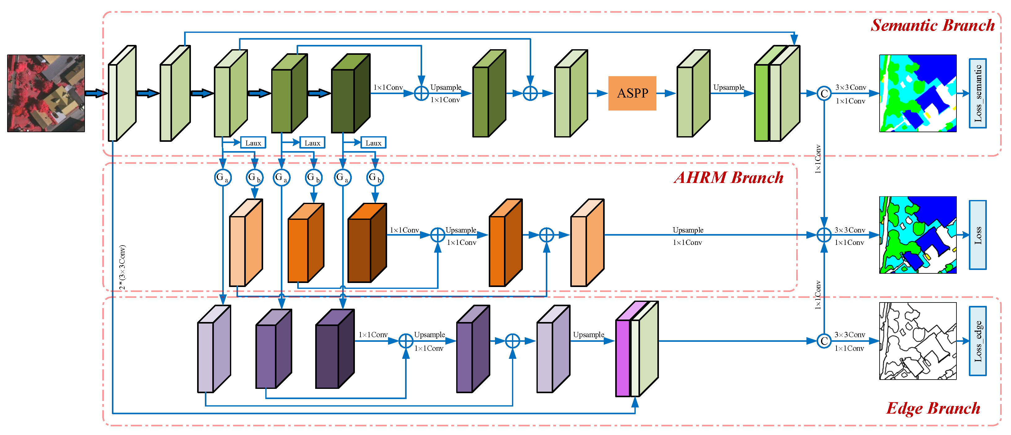
MBANet uses ResNet50 as the backbone network and replaces the normal convolution of the last block with atrous convolution to extract feature maps with higher resolution (output stride = 16). MBANet consists of three branches in parallel, namely, a semantic branch, an AHRM branch, and an edge branch, as shown in Figure 1.
The semantic branch uses ResNet50 as the backbone to formulate an FPN for extracting hierarchical multi-scale semantic features, which are then fed to an ASPP module to capture multi-scale contextual information. Following the idea of DeepLab, the low-level features of the first block of ResNet are added to the outputs of ASPP to enrich the extracted contextual information. The AHRM branch exploits an entropy-based gating mechanism that adaptively mines hard regions from the outputs of the last three blocks of ResNet to enhance the features of these hard regions. Finally, the enhanced multi-scale feature outputs from the three blocks are integrated with FPN to obtain the salient features of hard regions. Similarly, the edge branch uses another gating mechanism based on the prediction confusion map (PCM) [50] to explicitly extract object edges from the outputs of the last three blocks of ResNet, after which the multi-scale edge features are aggregated in FPN. Finally, to enrich the detailed spatial information, the aggregated features are combined with the features of the convolutional layer of ResNet. The features extracted by these three branches have complementary properties. Therefore, the final features of MBANet are simply the sum of these three sets of features. The final features are passed through the and convolutional layers to perform classification and finally upsampled to generate prediction results. Details of each branch are described in the following subsections.
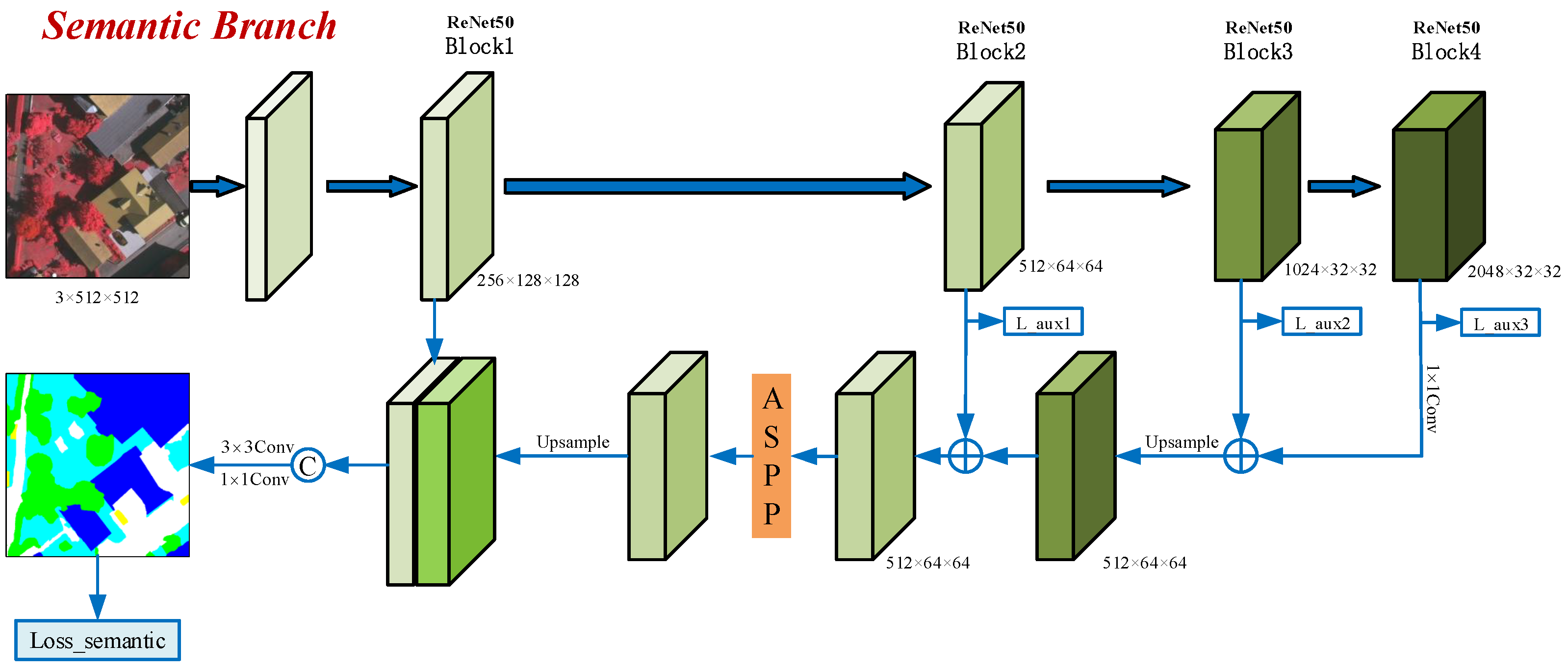
3.2. Semantic Branch
The semantic branch is the main branch of MBANet, which aims to extract multi-scale features that are very important for the accurate segmentation of objects with different scales. To balance feature representation capability, computational complexity, and memory footprint, we choose ResNet50 as the backbone network. In order to maintain an effective representation of small objects (e.g., cars), the DeepLab series [17,18,19] replaces conventional convolutions in the last two blocks of ResNet with atrous convolutions (output stride = 8) to obtain high-resolution feature maps. Subsequently, the ASPP module is concatenated to capture multi-scale contextual information. To reduce memory footprint, MBANet uses atrous convolution as a substitute for the conventional convolution in the last block of ResNet (output stride = 16). Meanwhile, in order to obtain higher resolution feature maps, we utilize an FPN to aggregate the features of the last three blocks of ResNet. This approach can not only aggregate multi-scale features to a certain extent, but also increase the resolution of feature maps (equivalent to output stride = 8) while having fewer channels (1/4 of the fourth block of ResNet). Compared to the DeepLab series, this method significantly reduces the number of feature map input channels to the ASPP module, and therefore decreases computational cost and memory usage. The features obtained by the ASPP module are concatenated with those of the first block of ResNet. Then, their channels are decreased to 64 by convolution. The final feature of MBANet is obtained by fusing the 64-channel features and the output features of the other two branches. To provide explicit supervision to the semantic branch, the 64-channel features are smoothed with and convolutional layers and upsampled to obtain semantic segmentation results. Lastly, the semantic loss (Loss_semantic in Figure 2) is computed over the segmentation results and labels.
Apart from this, we utilize the feature maps of the last three blocks of ResNet to make coarse auxiliary predictions and set an auxiliary loss for each block (Loss_aux1, Loss_aux2, and Loss_aux3 in Figure 2).
This setting serves two purposes. On one hand, it can provide deep supervision for the backbone network with the help of separately designed losses for different blocks. On the other hand, the coarse predictions in the setting act as the basis of the two gating mechanisms used in the other two branches.
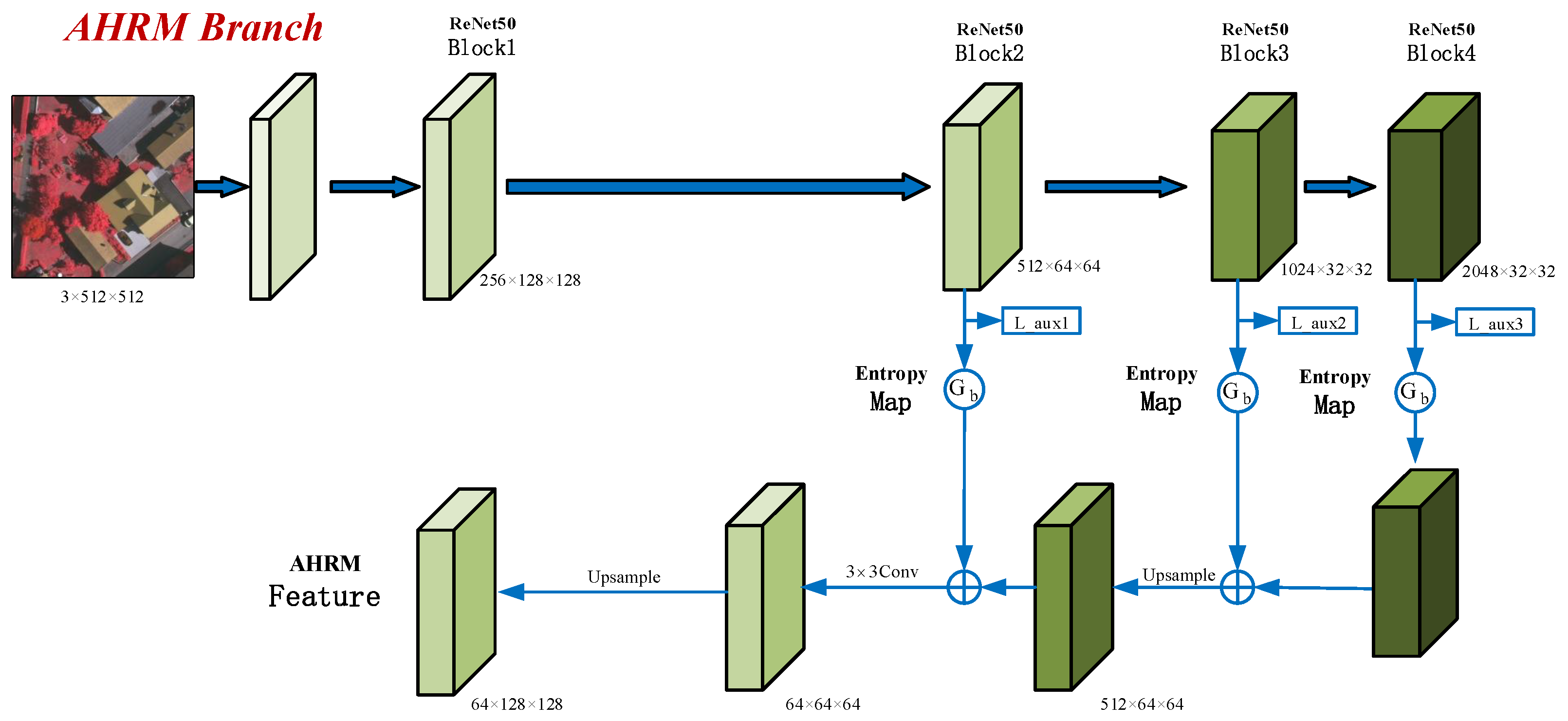
3.3. AHRM Branch
The goal of the AHRM branch is to explicitly extract the features of hard regions from the outputs of the last three blocks of ResNet as showen in Figure 3. Therefore, effectively measuring the classification difficulty of each sample is the key to hard region mining. As mentioned above, we use the last three blocks of ResNet for coarse prediction. As with the final segmentation results, the coarse results consist of six channels at a given location, corresponding to the probabilities of the six classes in the dataset. We will use the entropy of the six channels, represented as a vector, to measure the classification difficulty of a sample, because high entropy implies low prediction stability, and vice versa.
We calculate the entropy of the three auxiliary prediction results for every pixel and thus obtain three entropy maps. Pixels with higher entropy in the maps are harder to classify. We downsample the three entropy maps to obtain the gating unit of each block. The features of each block are then multiplied by the value of the corresponding gate to highlight the features of hard regions in the image. Features of hard regions with different resolutions from the three blocks are aggregated by the FPN. Finally, the aggregated features are reduced to 64 channels by convolution and upsampled to restore their resolution. These 64-channel hard region feature maps are part of the final feature maps of MBANet.
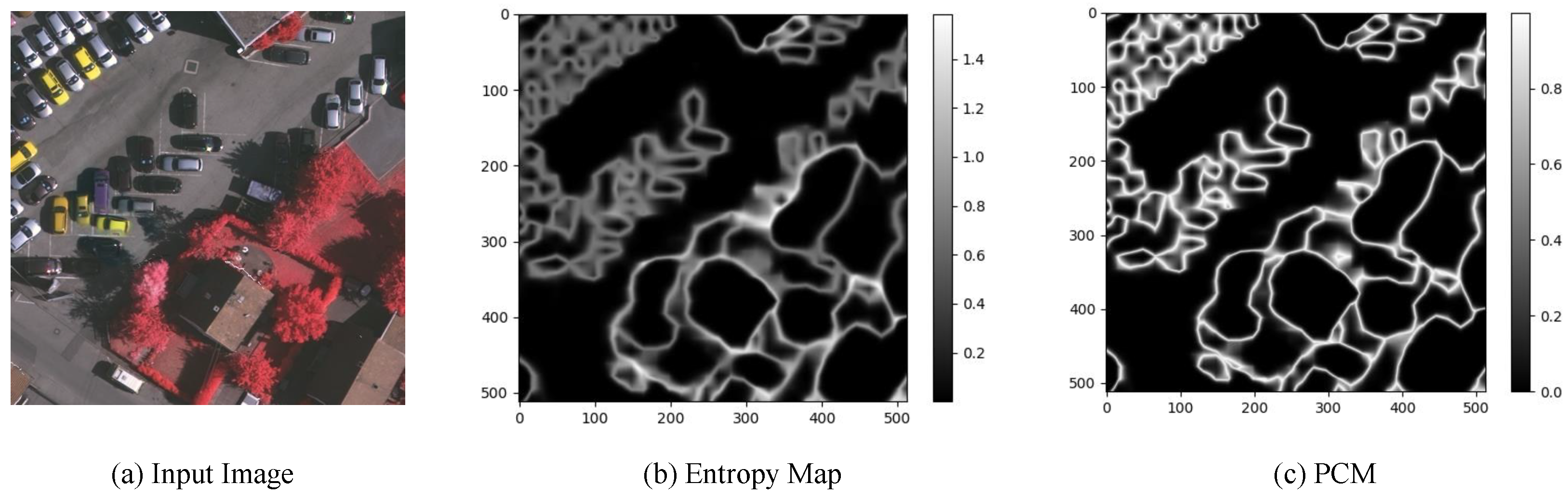
As shown in Figure 4b, we have visualized the entropy map of the prediction results of the last block’s auxiliary branch so as to gain a deeper understanding of the method. The entropy of each pixel in this image ranges from 0 to 1.6. Observing the entropy maps of all the test images, we empirically found that the value range stabilizes in the range of (0, 1.8). Samples with higher entropy are continuously distributed around the boundary to form connected regions. The brighter regions in the image have higher entropy, which means that the prediction uncertainty for the region is higher and, therefore, more difficult to classify accurately. It can be seen that these regions are mostly distributed near the edges. Note that the upper left part of the entropy map is brighter except for the edge regions. It can be found in the input image that many cars are parked in this area. The close arrangement of these cars and the interference of shadows make it difficult to parse this area accurately. The AHRM branch uses the entropy map as a gating unit, which multiplies pixel-by-pixel feature map outputs by different blocks of ResNet so as to enhance features in hard regions while suppressing features in easy regions.
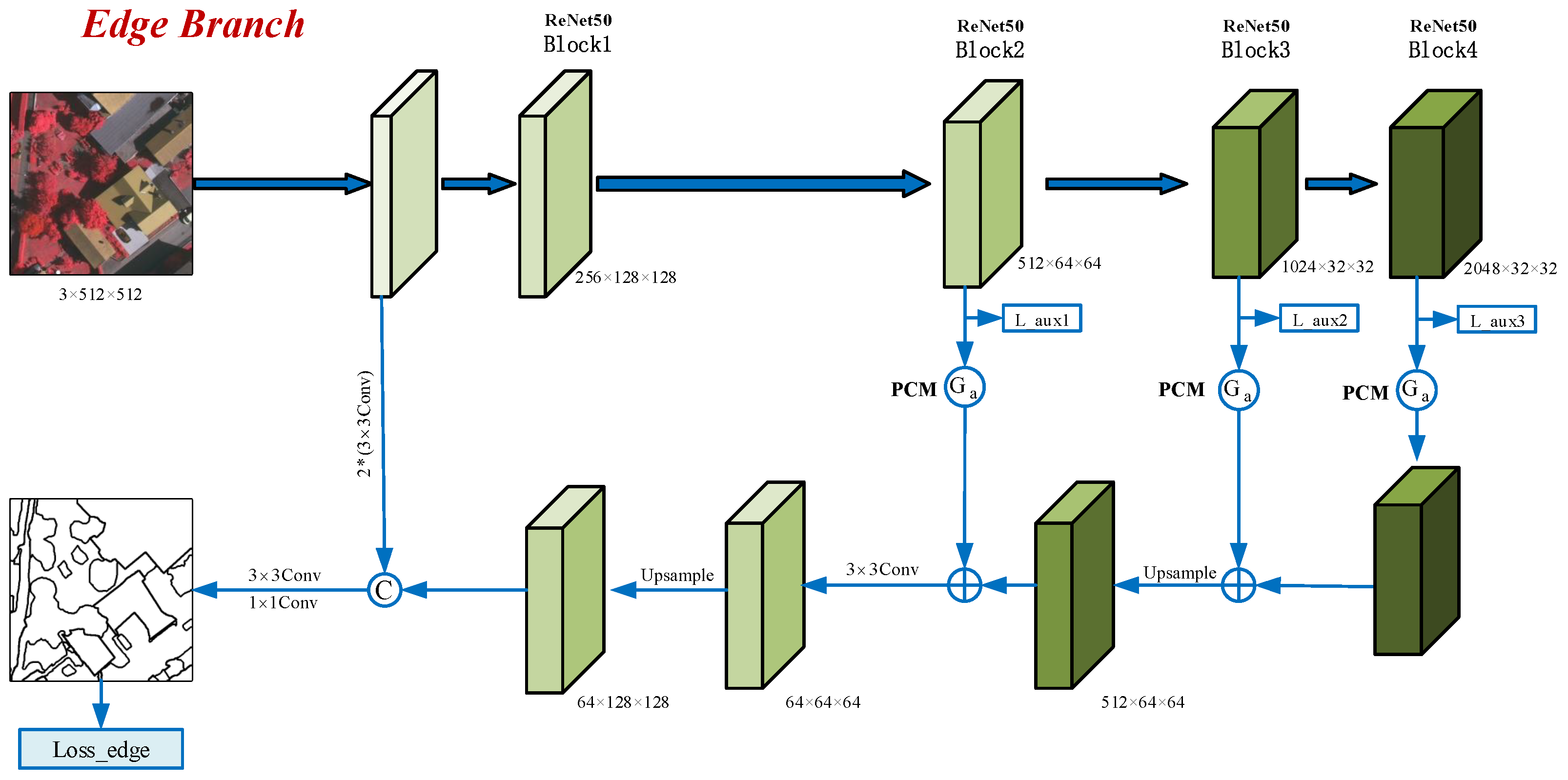
3.4. Edge Branch
It can be seen that hard regions (i.e., brighter regions in Figure 4b) mostly cluster around the edges. These hard-to-classify regions are very difficult to train with direct supervision. In this work, we elaborately devise an edge branch to extract edge features explicitly which is shown in Figure 5. In prior approaches, the most commonly used edge-extraction method is to learn edge information from the intermediate layers through a simple convolutional layer [22,44]. These learnable convolution kernels perform feature extraction on all pixels equally in the feature map and are combined with an edge loss (e.g., BCE loss) to guide model training. The method of feature learning used by these methods has a certain blindness. However, the fundamental driver for learning edge features with convolutional kernels is edge loss supervision. Therefore, in this paper, we manage to remove this blindness.
Our previous work [50] proposed a prediction confusion map (PCM), as shown in Figure 4c, which is generated through the following steps. (1) For a given pixel, sort the predicted logits; (2) take the difference between the top two maxima; (3) reverse this difference to obtain the prediction confusion of the pixel; (4) extend these operations to all pixels in the image to yield a PCM.
Unlike the entropy map calculation method, a PCM is obtained from only the top two maxima in the prediction logits, corresponding to the probabilities of the two most likely classes of the pixel. The PCM uses the inversion of the difference between these two maxima to measure the prediction confusion of each pixel. The smaller the difference is, the more difficult it is to classify the corresponding pixels. It is difficult to predict the brighter points of the PCM accurately because of the inversion operation. As shown in Figure 4c, most of the highly confusing pixels are concentrated around the edges. Furthermore, compared with the ambiguous representation of edges by the entropy map of Figure 4b, the PCM highlights the object boundaries more clearly. As a result, the PCM can effectively represent edges in prediction results. Inspired by this, we utilize a PCM as the gating unit of the edge branch to capture edge information from intermediate feature maps. The edge gating mechanism can effectively tackle the blindness of indiscriminate feature learning.
Similar to the AHRM branch, we compute the PCMs based on the predictions of the last three blocks of ResNet and downsample them as the edge-extraction gating units. The gating units are multiplied by the outputs of the corresponding blocks to extract edge information from intermediate layer features explicitly. Finally, the edge features of different resolutions are aggregated by an FPN. The features obtained by the first convolutional layer of ResNet contain many spatial details, which can make up for the insufficient representation of boundary details in the intermediate layers of ResNet. We use two convolutional layers to filter out redundant details and concatenate them with the aggregated edge features. Subsequently, their channels are reduced to 64 by a convolutional layer, and their resolution is restored by upsampling. These 64-channel edge feature maps are part of the final feature of MBANet.
To provide explicit supervision for the edge branch, we use a and a convolutional layer to obtain edge prediction results on the final edge features, and calculate the edge loss between the edge prediction and the edge labels. Specifically, since edge prediction is a binary classification task, a binary cross-entropy (BCE) loss is employed in this branch. We extract the boundaries of objects from the ground truth to construct edge labels.
3.5. Loss Function
The proposed MBANet consists of three parallel network branches. Apart from the loss of the final result, both the semantic branch and the edge branch have loss supervision. Furthermore, auxiliary losses are set for the last three blocks of the backbone network—ResNet. Therefore, the final loss () consists of six parts, among which the loss of the final result of the network (), the loss of the semantic branch (), and the other three auxiliary losses (, , and ) are all cross-entropy losses. A BCE loss () is used to supervise training in the edge branch. We set a weighting factor to balance the proportion of auxiliary losses. Additionally, we performed ablation studies on the Vaihingen dataset, and eventually found the optimal value of . Therefore, the final loss is formulated as
4. Experiments and Results
We detail the two HRRSI semantic segmentation datasets from ISPRS and the specific experimental setting.
4.1. Datasets
The ISPRS Vaihingen and Potsdam datasets were employed for experimental validation. These two datasets are sampled from the orthographic projection maps of the cities of Vaihingen and Potsdam in Germany, which contain many typical urban scenes. Vaihingen is a small village with numerous independent buildings. Potsdam, on the other hand, is a relatively large city with many dense and large buildings. Therefore, the characteristics of the two datasets are significantly different and represent different styles of urban scenes. The images are annotated into six classes: Impervious surfaces, Building, Low vegetation, Tree, Car, and Clutter/background. Since the size of the original images is too large for training, we used a sliding window method to cut them into small patches of size . In addition, we set an overlap ratio of 1/3 for the sliding window for the training images. We present the two datasets in detail in Table 1, including the size of the original large images, the ground sampling distance (GSD), wave bands, scenes, and the number of original large images and small patches.
4.2. Experiment Setup
The detailed experimental setup is shown in Table 2. Following the settings of [17], we use the Poly learning strategy to speed up the model convergence, which is expressed as
Following the settings of [50], this paper uses multiple metrics to measure model performance, including OA, mIoU, and mean , as well as IoU score and score for each class.
4.3. Ablation Study
The effectiveness of each branch is verified in this section. Further, the effectiveness of the gating mechanism in the AHRM branch and the edge branch is verified. Finally, the optimal value of the auxiliary loss weight is studied.
4.3.1. Ablation Study for the Semantic Branch
This paper utilizes atrous convolution to replace the conventional convolution in the third and fourth blocks of ResNet50 (output stride = 8) as a backbone to build a fully convolutional network (FCN) as the baseline model. Since the structure of the semantic branch is similar to DeepLab v3+, we compare its performance with FCN and DeepLab v3+. We calculate the and IoU scores for each class separately, as well as the final OA, mean , and mIoU scores, and further count their memory usage. The experimental results are presented in Table 3. Our semantic branch achieved the best results except for Car. This is because the features extracted by ResNet used in DeepLab v3+ have higher resolution (output stride = 8), which better preserves the semantic information of the small-scale class of Car. However, although our method sacrifices accuracy for Car, it greatly reduces the GPU memory usage and therefore achieve, outstanding results.
Additionally, in this subsection, we investigate the influence of deep supervision provided by auxiliary losses on the semantic branch. We empirically set and performed experimental validation on the Vaihingen dataset. The experimental results are displayed in Table 4. Undoubtedly, the auxiliary loss can positively impact the semantic branch. Therefore, all of our subsequent experiments retain these three auxiliary losses.
4.3.2. Ablation Study for the AHRM Branch
In this section, we study the semantic and AHRM branches’ compatibility and further verify the gating mechanism’s effectiveness in the AHRM branch. Based on the semantic branch, we add AHRM branches without or with gating units, and test their performance on the Vaihingen test set. The experimental results are illustrated in Table 5.
The model’s performance can be slightly improved by simply aggregating the features of the intermediate layers and concatenating them with the features extracted by the semantic branch. Furthermore, with the assistance of the proposed gating unit, the model’s performance is significantly improved.
However, the addition of the AHRM branch slightly increases the memory usage of the GPU. In the experimental results, all classes except Car obtained the highest scores, which verifies the effectiveness of the AHRM branch and the gating mechanism based on the entropy map. This may be because the entropy map does not adequately represent the edges of cars. Therefore, we try to explore solutions from the edge branch.
4.3.3. Ablation Study for the Edge Branch
Similar to the AHRM branch, in this section, we study the compatibility of the semantic and the edge branches and further demonstrate the effectiveness of the gating mechanism in the edge branch. We add edge branches without or with gating units based on the semantic branch and test their performance on the Vaihingen test set. The experimental results are provided in Table 6.
The experimental results of the edge branch are consistent with the AHRM branch. Adding an edge branch without gating units can slightly improve model performance, and with gating units, the improvement is greater. Moreover, the edge branches take up little GPU memory. Experimental results show that all classes except Building achieve the highest scores, demonstrating the effectiveness of the edge branch and the gating mechanism based on PCM. This may be because the edge features of buildings are relatively fixed (usually rectangular) and are easier to extract even without edge supervision. It should be noted that compared with the AHRM branch, the addition of the edge branch can effectively improve the accuracy for cars, which can make up for the deficiency of the AHRM branch.
4.3.4. Integration of the Three Branches
In this section, we integrate three branches to build the MBANet. Considering that the results of auxiliary predictions inevitably influence the model performance (since gating units are derived from them), we conducted a series of experiments to compare the performance when different weights of the auxiliary loss on the Vaihingen dataset are used. The results are summarized in Table 7. It demonstrates that our network achieved the best results when . Notably, the model obtained the worst results when . In this case, the auxiliary branch loses the supervision information, so the gating unit cannot effectively select specific features. On the contrary, it introduces significant noise to the features of the semantic branch, resulting in poor model performance.
We sorted the three branches’ experimental results and counted their memory footprint. The final results are summarized in Table 8, which demonstrates that the three branches in our model are compatible and that their features complement each other. The other two branches occupy little memory storage, which is convenient for deployment and training.
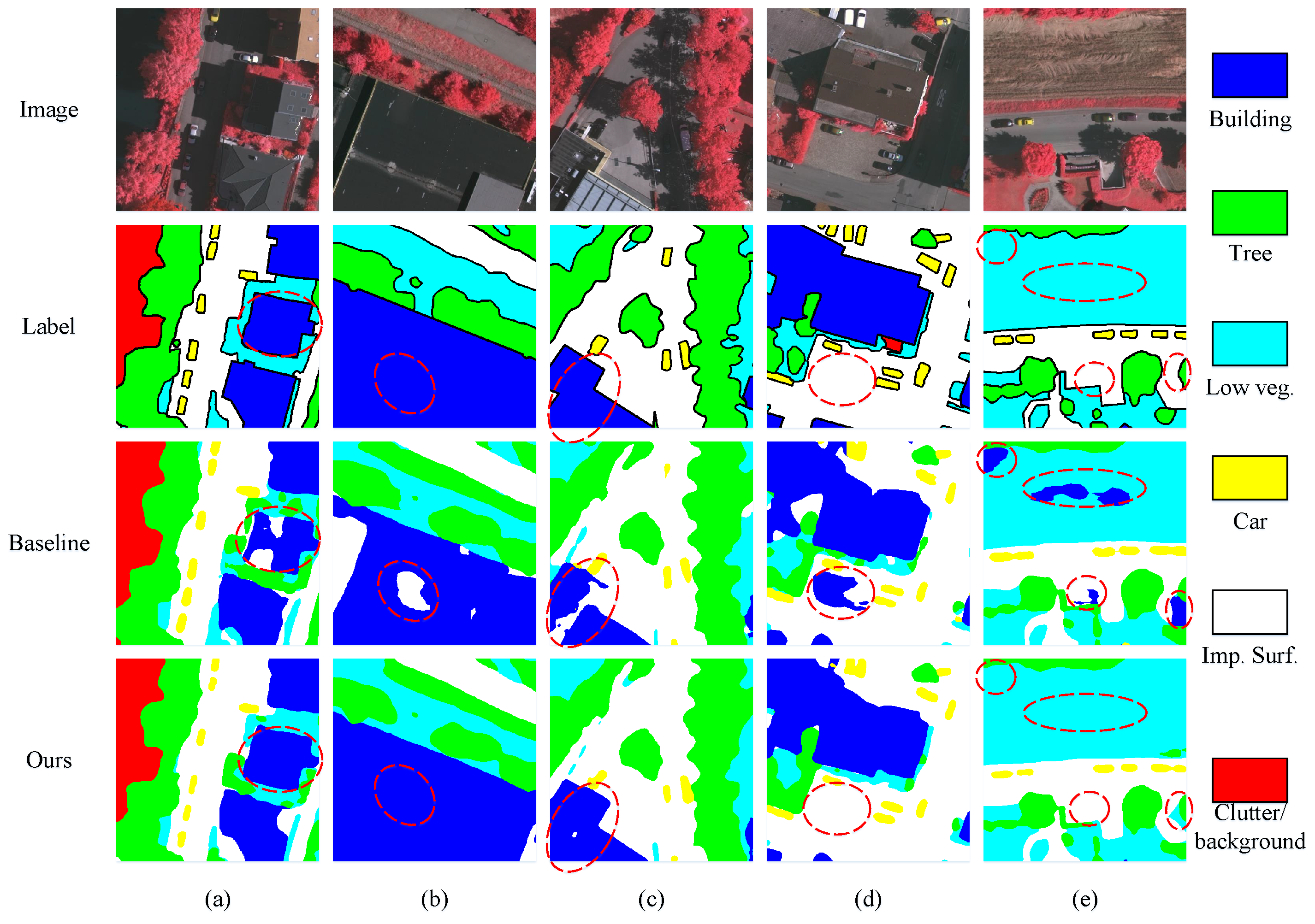
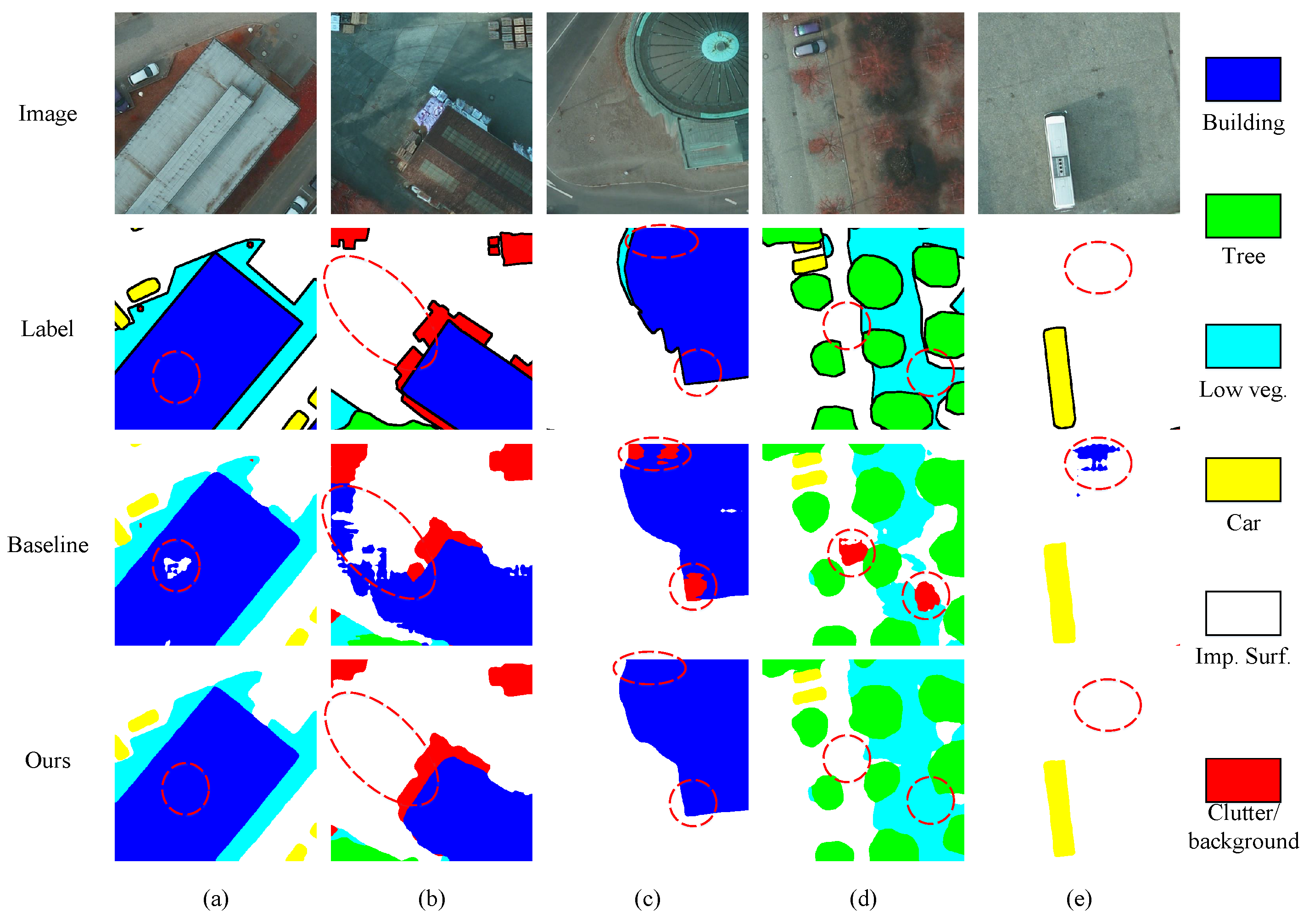
As a complement, we demonstrate the effectiveness of our method on the Potsdam dataset. The experimental results are summarized in Table 9. Compared to the baseline, the OA, mean , and mIoU scores are improved by 1.91%, 2.59%, and 3.94%, respectively, on the Vaihingen dataset, while on the Potsdam dataset, the improvement rates are 1.14%, 1.7%, and 2.4%, respectively. For intuitive understanding, we visualized the prediction results of some small patches and marked the advantageous regions with red dotted ellipses, as shown in Figure 6 and Figure 7.
4.4. Comparison with Other SOTA Methods
This section compares the performance of MBANet with other SOTA methods. Furthermore, we compare the computational complexity of the model with some commonly used methods.
The previous experiments in this paper were conducted on small patches of size . This section tests the performance of MBANet on the original large images. Since the original images are too large to test, we use the sliding window (SW) method for testing. We set an overlap ratio of 1/3 for each sliding window to prevent tearing when the predicted small patches are stitched together. Furthermore, we use multi-scale testing (MS) and flipping (Flip) to improve the model generalization ability. To compare with other methods, we only calculated five classes, excluding Clutter, when computing mIoU and mean scores on the original large image.
We performed ablation studies on three test augmentation methods. The experimental results are recorded in Table 10 and Table 11. We can see that each method is very effective in improving the model’s performance. Additionally, comparison results with other SOTA methods are recorded in Table 12 and Table 13.
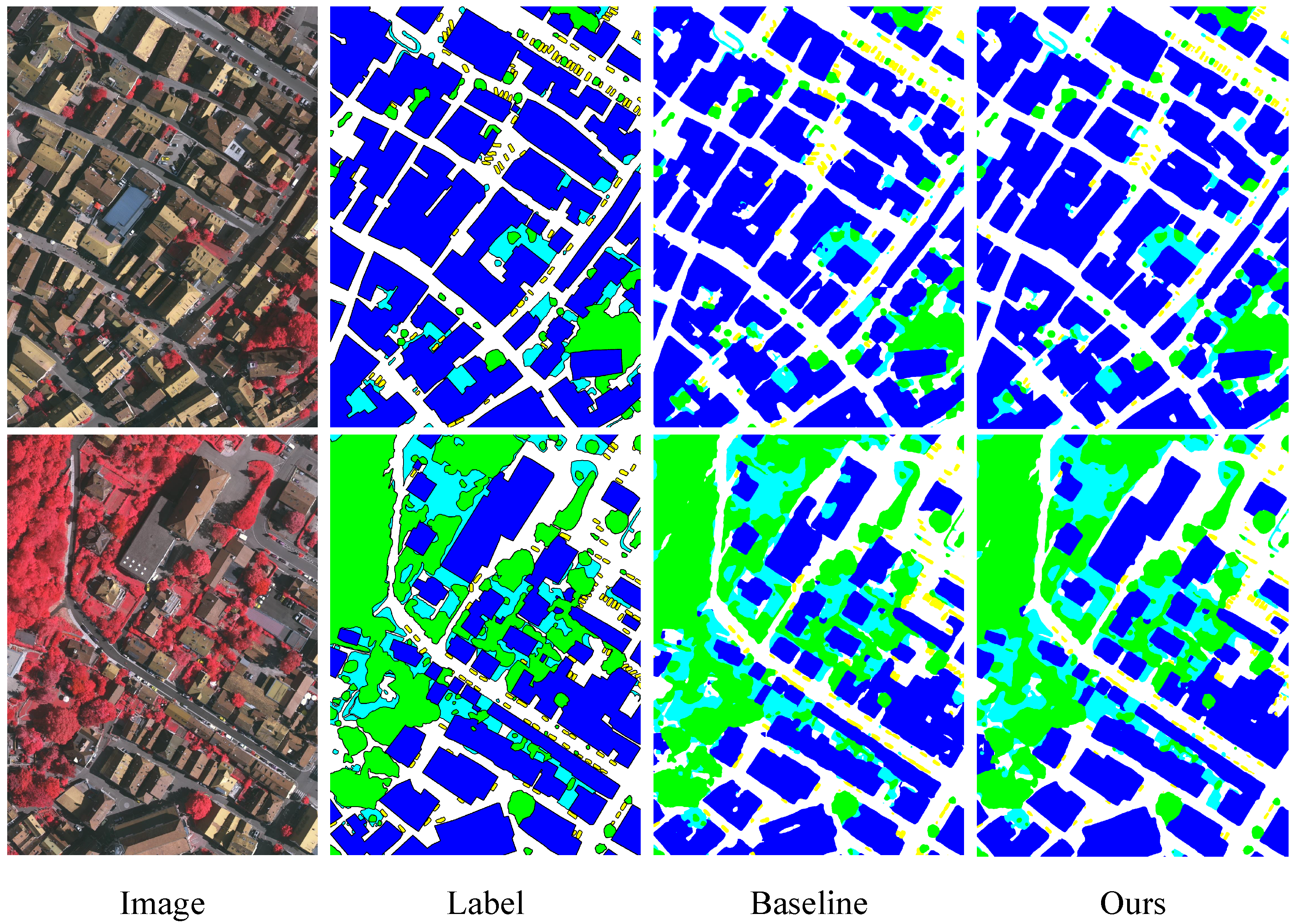
For the Vaihingen dataset, our MBANet achieved the highest scores on all classes except Car, and the OA, mean , and mIoU scores all exhibited SOTA performance. For the Potsdam dataset, scores for all classes except Impervious surfaces and Building reached SOTA level. We visualized the prediction results on the original large images and illustrate them in Figure 8 and Figure 9.
4.5. Model Complexity Analysis
Our MBANet is suspected of being too complex because it contains three network branches. Therefore, we compared the computational complexity of MBANet with other well-known networks. The comparison results are shown in Table 14. Due to the multi-branch structure, our network inevitably has more parameters than other models. However, benefiting from the setting of output stride = 16 in the backbone, much computational work in the network is concentrated on feature maps with smaller resolutions, which enormously reduces the computational complexity.
5. Conclusions
This paper proposes a multi-branch adaptive hard region mining network for urban scene parsing of HRRSIs. The network consists of three branches: a semantic branch, an adaptive hard region mining branch, and an edge branch. First, a multi-scale semantic branch is designed to effectively extract multi-scale features of objects with varying sizes in urban scenes. Secondly, a gating mechanism based on the entropy map is proposed, which can adaptively mine the hard-to-classify regions in the images and construct an adaptive hard region mining branch. Furthermore, to extract the edges of objects explicitly, an edge gating mechanism based on a prediction confusion map (PCM) is proposed to formulate an edge branch. The experimental results on the ISPRS Vaihingen and Potsdam datasets demonstrate that the features extracted by the three branches can complement each other and are compatible. In addition, the proposed method is evaluated on the original large-scale images of two datasets, and its computational complexity is compared with prior works. Our network has an advantage in computational complexity, despite having more model parameters due to its sophisticated design philosophy. Experiments show that our method can achieve SOTA performance on two high-resolution urban scene semantic labeling datasets from ISPRS. Although MBANet achieves outstanding performance, the model has a large number of parameters. Our future work will focus on designing lightweight models to achieve high-accuracy urban scene parsing.
Author Contributions
Investigation, Y.Z. and H.B.; methodology, H.B.; project administration, J.C.; software, Y.S. and H.B.; visualization, Q.W. and H.B.; writing—review and editing, H.H. and H.B. All authors have read and agreed to the published version of the manuscript.
Funding
This research was supported by the National Natural Science Foundation of China (No. 62071104), and partly supported by the NNSFC and CAAC (No. U2133211).
Institutional Review Board Statement
Not applicable.
Informed Consent Statement
Not applicable.
Data Availability Statement
We used two public 2D semantic labeling datasets, Vaihingen and Potsdam, provided by the International Society for Photogrammetry and Remote Sensing(ISPRS), https://www2.isprs.org/commissions/comm2/wg4/benchmark/semantic-labeling/, accessed on 29 March 2019.
Conflicts of Interest
The authors declare no conflict of interest.
References
- Peng, D.; Zhang, Y.; Guan, H. End-to-end change detection for high resolution satellite images using improved UNet++. Remote Sens. 2019, 11, 1382. [Google Scholar] [CrossRef] [Green Version]
- Fang, B.; Pan, L.; Kou, R. Dual learning-based siamese framework for change detection using bi-temporal VHR optical remote sensing images. Remote Sens. 2019, 11, 1292. [Google Scholar] [CrossRef] [Green Version]
- Chen, H.; Wu, C.; Du, B.; Zhang, L.; Wang, L. Change detection in multisource VHR images via deep siamese convolutional multiple-layers recurrent neural network. IEEE Trans. Geosci. Remote Sens. 2019, 58, 2848–2864. [Google Scholar] [CrossRef]
- Willis, K. Remote sensing change detection for ecological monitoring in United States protected areas. Biol. Conserv. 2015, 182, 233–242. [Google Scholar] [CrossRef]
- Shan, W.; Jin, X.; Ren, J.; Wang, Y.; Xu, Z.; Fan, Y.; Gu, Z.; Hong, C.; Lin, J.; Zhou, Y. Ecological environment quality assessment based on remote sensing data for land consolidation. J. Clean. Prod. 2019, 239, 118126. [Google Scholar] [CrossRef]
- Boni, G.; De Angeli, S.; Taramasso, A.; Roth, G. Remote sensing-based methodology for the quick update of the assessment of the population exposed to natural hazards. Remote Sens. 2020, 12, 3943. [Google Scholar] [CrossRef]
- Gillespie, T.; Chu, J.; Frankenberg, E.; Thomas, D. Assessment and prediction of natural hazards from satellite imagery. Prog. Phys. Geogr. 2007, 31, 459–470. [Google Scholar] [CrossRef] [Green Version]
- Ehrlich, D.; Melchiorri, M.; Florczyk, A.; Pesaresi, M.; Kemper, T.; Corbane, C.; Freire, S.; Schiavina, M.; Siragusa, A. Remote sensing derived built-up area and population density to quantify global exposure to five natural hazards over time. Remote Sens. 2018, 10, 1378. [Google Scholar] [CrossRef] [Green Version]
- Yi, Y.; Zhang, Z.; Zhang, W.; Zhang, C.; Li, W.; Zhao, T. Semantic segmentation of urban buildings from VHR remote sensing imagery using a deep convolutional neural network. Remote Sens. 2019, 11, 1774. [Google Scholar] [CrossRef] [Green Version]
- Grinias, I.; Panagiotakis, C.; Tziritas, G. MRF-based segmentation and unsupervised classification for building and road detection in peri-urban areas of high-resolution satellite images. Isprs J. Photogramm. Remote Sens. 2016, 122, 145–166. [Google Scholar] [CrossRef]
- Nezami, S.; Khoramshahi, E.; Nevalainen, O.; Pölönen, I.; Honkavaara, E. Tree species classification of drone hyperspectral and RGB imagery with deep learning convolutional neural networks. Remote Sens. 2020, 12, 1070. [Google Scholar] [CrossRef] [Green Version]
- Schiefer, F.; Kattenborn, T.; Frick, A.; Frey, J.; Schall, P.; Koch, B.; Schmidtlein, S. Mapping forest tree species in high resolution UAV-based RGB-imagery by means of convolutional neural networks. Isprs J. Photogramm. Remote Sens. 2020, 170, 205–215. [Google Scholar] [CrossRef]
- LeCun, Y.; Bengio, Y.; Hinton, G. Deep learning. Nature 2015, 521, 436–444. [Google Scholar] [CrossRef] [PubMed]
- Guo, Y.; Liu, Y.; Georgiou, T.; Lew, M. A review of semantic segmentation using deep neural networks. Int. J. Multimed. Inf. Retr. 2018, 7, 87–93. [Google Scholar] [CrossRef] [Green Version]
- Lin, T.; Dollár, P.; Girshick, R.; He, K.; Hariharan, B.; Belongie, S. Feature pyramid networks for object detection. In Proceedings of the IEEE Conference on Computer Vision and Pattern Recognition, Honolulu, HI, USA, 21–26 July 2017; pp. 2117–2125. [Google Scholar]
- Ronneberger, O.; Fischer, P.; Brox, T. U-net: Convolutional networks for biomedical image segmentation. In Proceedings of the International Conference on Medical Image Computing and Computer-Assisted Intervention, Munich, Germany, 5–9 October 2015; pp. 234–241. [Google Scholar]
- Chen, L.; Papandreou, G.; Kokkinos, I.; Murphy, K.; Yuille, A. Deeplab: Semantic image segmentation with deep convolutional nets, atrous convolution, and fully connected crfs. IEEE Trans. Pattern Anal. Mach. Intell. 2017, 40, 834–848. [Google Scholar] [CrossRef] [Green Version]
- Chen, L.; Papandreou, G.; Schroff, F.; Adam, H. Rethinking atrous convolution for semantic image segmentation. arXiv 2017, arXiv:1706.05587. [Google Scholar]
- Chen, L.; Zhu, Y.; Papandreou, G.; Schroff, F.; Adam, H. Encoder-decoder with atrous separable convolution for semantic image segmentation. In Proceedings of the European Conference on Computer Vision (ECCV), Munich, Germany, 8–14 September 2018; pp. 801–818. [Google Scholar]
- Zheng, X.; Huan, L.; Xia, G.; Gong, J. Parsing very high resolution urban scene images by learning deep ConvNets with edge-aware loss. Isprs J. Photogramm. Remote Sens. 2020, 170, 15–28. [Google Scholar] [CrossRef]
- Milletari, F.; Navab, N.; Ahmadi, S. V-net: Fully convolutional neural networks for volumetric medical image segmentation. In Proceedings of the 2016 Fourth International Conference on 3D Vision (3DV), Stanford, CA, USA, 25–28 October 2016; pp. 565–571. [Google Scholar]
- Chen, F.; Liu, H.; Zeng, Z.; Zhou, X.; Tan, X. BES-Net: Boundary Enhancing Semantic Context Network for High-Resolution Image Semantic Segmentation. Remote Sens. 2022, 14, 1638. [Google Scholar] [CrossRef]
- Shrivastava, A.; Gupta, A.; Girshick, R. Training region-based object detectors with online hard example mining. In Proceedings of the IEEE Conference on Computer Vision and Pattern Recognition, Las Vegas, NV, USA, 27–30 June 2016; pp. 761–769. [Google Scholar]
- Kirillov, A.; Wu, Y.; He, K.; Girshick, R. Pointrend: Image segmentation as rendering. In Proceedings of the IEEE/CVF Conference on Computer Vision and Pattern Recognition, Seattle, WA, USA, 13–19 June 2020; pp. 9799–9808. [Google Scholar]
- Kim, S.; Kook, H.; Sun, J.; Kang, M.; Ko, S. Parallel feature pyramid network for object detection. In Proceedings of the European Conference on Computer Vision (ECCV), Munich, Germany, 8–14 September 2018; pp. 234–250. [Google Scholar]
- Cao, J.; Chen, Q.; Guo, J.; Shi, R. Attention-guided context feature pyramid network for object detection. arXiv 2020, arXiv:2005.11475. [Google Scholar]
- Li, X.; Lai, T.; Wang, S.; Chen, Q.; Yang, C.; Chen, R.; Lin, J.; Zheng, F. Weighted feature pyramid networks for object detection. In Proceedings of the 2019 IEEE Intl Conf on Parallel & Distributed Processing with Applications, Big Data & Cloud Computing, Sustainable Computing & Communications, Social Computing & Networking (ISPA/BDCloud/SocialCom/SustainCom), Xiamen, China, 16–18 December 2019; pp. 1500–1504. [Google Scholar]
- Li, X.; Zhao, H.; Han, L.; Tong, Y.; Tan, S.; Yang, K. Gated fully fusion for semantic segmentation. In Proceedings of the AAAI Conference on Artificial Intelligence, New York, NY, USA, 7–12 February 2020; Volume 34, pp. 11418–11425. [Google Scholar]
- Ye, M.; Ouyang, J.; Chen, G.; Zhang, J.; Yu, X. Enhanced Feature Pyramid Network for Semantic Segmentation. In Proceedings of the 2020 25th International Conference on Pattern Recognition (ICPR), Milan, Italy, 10–15 January 2021; pp. 3209–3216. [Google Scholar]
- Zhao, H.; Shi, J.; Qi, X.; Wang, X.; Jia, J. Pyramid scene parsing network. In Proceedings of the IEEE Conference on Computer Vision and Pattern Recognition, Honolulu, HI, USA, 21–26 July 2017; pp. 2881–2890. [Google Scholar]
- Yu, B.; Yang, L.; Chen, F. Semantic segmentation for high spatial resolution remote sensing images based on convolution neural network and pyramid pooling module. IEEE J. Sel. Top. Appl. Earth Obs. Remote Sens. 2018, 11, 3252–3261. [Google Scholar] [CrossRef]
- Wang, Y.; Chen, C.; Ding, M.; Li, J. Real-time dense semantic labeling with dual-Path framework for high-resolution remote sensing image. Remote Sens. 2019, 11, 3020. [Google Scholar] [CrossRef] [Green Version]
- Bai, Y.; Hu, J.; Su, J.; Liu, X.; Liu, H.; He, X.; Meng, S.; Mas, E.; Koshimura, S. Pyramid pooling module-based semi-siamese network: A benchmark model for assessing building damage from xBD satellite imagery datasets. Remote Sens. 2020, 12, 4055. [Google Scholar] [CrossRef]
- Su, Y.; Cheng, J.; Bai, H.; Liu, H.; He, C. Semantic Segmentation of Very-High-Resolution Remote Sensing Images via Deep Multi-Feature Learning. Remote Sens. 2022, 14, 533. [Google Scholar] [CrossRef]
- Loshchilov, I.; Hutter, F. Online batch selection for faster training of neural networks. arXiv 2015, arXiv:1511.06343. [Google Scholar]
- Yuan, Y.; Huang, L.; Guo, J.; Zhang, C.; Chen, X.; Wang, J. OCNet: Object context for semantic segmentation. Int. J. Comput. Vis. 2021, 129, 2375–2398. [Google Scholar] [CrossRef]
- Li, X.; Liu, Z.; Luo, P.; Change Loy, C.; Tang, X. Not all pixels are equal: Difficulty-aware semantic segmentation via deep layer cascade. In Proceedings of the IEEE Conference on Computer Vision and Pattern Recognition, Honolulu, HI, USA, 21–26 July 2017; pp. 3193–3202. [Google Scholar]
- Yin, J.; Xia, P.; He, J. Online hard region mining for semantic segmentation. Neural Process. Lett. 2019, 50, 2665–2679. [Google Scholar] [CrossRef]
- Li, X.; Li, T.; Chen, Z.; Zhang, K.; Xia, R. Attentively Learning Edge Distributions for Semantic Segmentation of Remote Sensing Imagery. Remote Sens. 2021, 14, 102. [Google Scholar] [CrossRef]
- Sun, X.; Xia, M.; Dai, T. Controllable Fused Semantic Segmentation with Adaptive Edge Loss for Remote Sensing Parsing. Remote Sens. 2022, 14, 207. [Google Scholar] [CrossRef]
- Liu, Z.; Li, J.; Song, R.; Wu, C.; Liu, W.; Li, Z.; Li, Y. Edge Guided Context Aggregation Network for Semantic Segmentation of Remote Sensing Imagery. Remote Sens. 2022, 14, 1353. [Google Scholar] [CrossRef]
- Pan, S.; Tao, Y.; Nie, C.; Chong, Y. PEGNet: Progressive edge guidance network for semantic segmentation of remote sensing images. IEEE Geosci. Remote Sens. Lett. 2020, 18, 637–641. [Google Scholar] [CrossRef]
- Nong, Z.; Su, X.; Liu, Y.; Zhan, Z.; Yuan, Q. Boundary-Aware Dual-Stream Network for VHR Remote Sensing Images Semantic Segmentation. IEEE J. Sel. Top. Appl. Earth Obs. Remote Sens. 2021, 14, 5260–5268. [Google Scholar] [CrossRef]
- Jung, H.; Choi, H.; Kang, M. Boundary enhancement semantic segmentation for building extraction from remote sensed image. IEEE Trans. Geosci. Remote Sens. 2021, 60, 5215512. [Google Scholar] [CrossRef]
- He, C.; Li, S.; Xiong, D.; Fang, P.; Liao, M. Remote sensing image semantic segmentation based on edge information guidance. Remote Sens. 2020, 12, 1501. [Google Scholar] [CrossRef]
- Zhang, C.; Jiang, W.; Zhao, Q. Semantic segmentation of aerial imagery via split-attention networks with disentangled nonlocal and edge supervision. Remote Sens. 2021, 13, 1176. [Google Scholar] [CrossRef]
- Zhuang, C.; Yuan, X.; Wang, W. Boundary enhanced network for improved semantic segmentation. In Proceedings of the International Conference on Urban Intelligence and Applications, Taiyuan, China, 14–16 August2020; pp. 172–184. [Google Scholar]
- Liu, S.; Ding, W.; Liu, C.; Liu, Y.; Wang, Y.; Li, H. ERN: Edge loss reinforced semantic segmentation network for remote sensing images. Remote Sens. 2018, 10, 1339. [Google Scholar] [CrossRef] [Green Version]
- Zheng, X.; Huan, L.; Xiong, H.; Gong, J. ELKPPNet: An edge-aware neural network with large kernel pyramid pooling for learning discriminative features in semantic segmentation. arXiv 2019, arXiv:1906.11428. [Google Scholar]
- Bai, H.; Cheng, J.; Su, Y.; Liu, S.; Liu, X. Calibrated Focal Loss for Semantic Labeling of High-Resolution Remote Sensing Images. IEEE J. Sel. Top. Appl. Earth Obs. Remote Sens. 2022, 15, 6531–6547. [Google Scholar] [CrossRef]
- Volpi, M.; Tuia, D. Dense semantic labeling of subdecimeter resolution images with convolutional neural networks. IEEE Trans. Geosci. Remote Sens. 2016, 55, 881–893. [Google Scholar] [CrossRef] [Green Version]
- Marcos, D.; Volpi, M.; Kellenberger, B.; Tuia, D. Land cover mapping at very high resolution with rotation equivariant CNNs: Towards small yet accurate models. Isprs J. Photogramm. Remote Sens. 2018, 145, 96–107. [Google Scholar] [CrossRef] [Green Version]
- Mou, L.; Hua, Y.; Zhu, X. Relation matters: Relational context-aware fully convolutional network for semantic segmentation of high-resolution aerial images. IEEE Trans. Geosci. Remote Sens. 2020, 58, 7557–7569. [Google Scholar] [CrossRef]
- Nogueira, K.; Dalla Mura, M.; Chanussot, J.; Schwartz, W.; Dos Santos, J. Dynamic multicontext segmentation of remote sensing images based on convolutional networks. IEEE Trans. Geosci. Remote Sens. 2019, 57, 7503–7520. [Google Scholar] [CrossRef] [Green Version]
- Audebert, N.; Le Saux, B.; Lefèvre, S. Beyond RGB: Very high resolution urban remote sensing with multimodal deep networks. Isprs J. Photogramm. Remote Sens. 2018, 140, 20–32. [Google Scholar] [CrossRef] [Green Version]
- Marmanis, D.; Schindler, K.; Wegner, J.; Galliani, S.; Datcu, M.; Stilla, U. Classification with an edge: Improving semantic image segmentation with boundary detection. Isprs J. Photogramm. Remote Sens. 2018, 135, 158–172. [Google Scholar] [CrossRef] [Green Version]
- Yue, K.; Yang, L.; Li, R.; Hu, W.; Zhang, F.; Li, W. TreeUNet: Adaptive tree convolutional neural networks for subdecimeter aerial image segmentation. Isprs J. Photogramm. Remote Sens. 2019, 156, 1–13. [Google Scholar] [CrossRef]
- Fu, J.; Liu, J.; Tian, H.; Li, Y.; Bao, Y.; Fang, Z.; Lu, H. Dual attention network for scene segmentation. In Proceedings of the IEEE/CVF Conference on Computer Vision and Pattern Recognition, Long Beach, CA, USA, 15–20 June 2019; pp. 3146–3154. [Google Scholar]
- Zhang, F.; Chen, Y.; Li, Z.; Hong, Z.; Liu, J.; Ma, F.; Han, J.; Ding, E. Acfnet: Attentional class feature network for semantic segmentation. In Proceedings of the IEEE/CVF International Conference on Computer Vision, Seoul, Korea, 27 October–2 November 2019; pp. 6798–6807. [Google Scholar]
- Liu, Y.; Fan, B.; Wang, L.; Bai, J.; Xiang, S.; Pan, C. Semantic labeling in very high resolution images via a self-cascaded convolutional neural network. Isprs J. Photogramm. Remote Sens. 2018, 145, 78–95. [Google Scholar] [CrossRef] [Green Version]
- Huang, Z.; Wang, X.; Huang, L.; Huang, C.; Wei, Y.; Liu, W. Ccnet: Criss-cross attention for semantic segmentation. In Proceedings of the IEEE/CVF International Conference on Computer, Seoul, Korea, 27 October–2 November 2019; pp. 603–612. [Google Scholar]
- Ding, L.; Zhang, J.; Bruzzone, L. Semantic segmentation of large-size VHR remote sensing images using a two-stage multiscale training architecture. IEEE Trans. Geosci. Remote Sens. 2020, 58, 5367–5376. [Google Scholar] [CrossRef]
- Sun, Y.; Zhang, X.; Xin, Q.; Huang, J. Developing a multi-filter convolutional neural network for semantic segmentation using high-resolution aerial imagery and LiDAR data. Isprs J. Photogramm. Remote Sens. 2018, 143, 3–14. [Google Scholar] [CrossRef]
- Sun, Y.; Tian, Y.; Xu, Y. Problems of encoder-decoder frameworks for high-resolution remote sensing image segmentation: Structural stereotype and insufficient learning. Neurocomputing 2019, 330, 297–304. [Google Scholar] [CrossRef]
Figure 1.
The framework of our MBANet.

Figure 2.
The framework of the semantic branch.

Figure 3.
The framework of the AHRM branch.

Figure 4.
Visualization of the two gating mechanisms. (a) The input image of size . (b) The entropy map of the auxiliary prediction result of the last block of ResNet. The rightmost vertical axis represents the different entropy values in the image. The higher the brightness, the higher the entropy. (c) The PCM of the auxiliary prediction result of the last block of ResNet. The higher the brightness, the higher the prediction confusion.

Figure 5.
The framework of the edge branch.

Figure 6.
Visualization of the prediction results of different methods on the Vaihingen dataset. (a–e) correspond to five different input images, labels and segmentation results.
Figure 6.
Visualization of the prediction results of different methods on the Vaihingen dataset. (a–e) correspond to five different input images, labels and segmentation results.

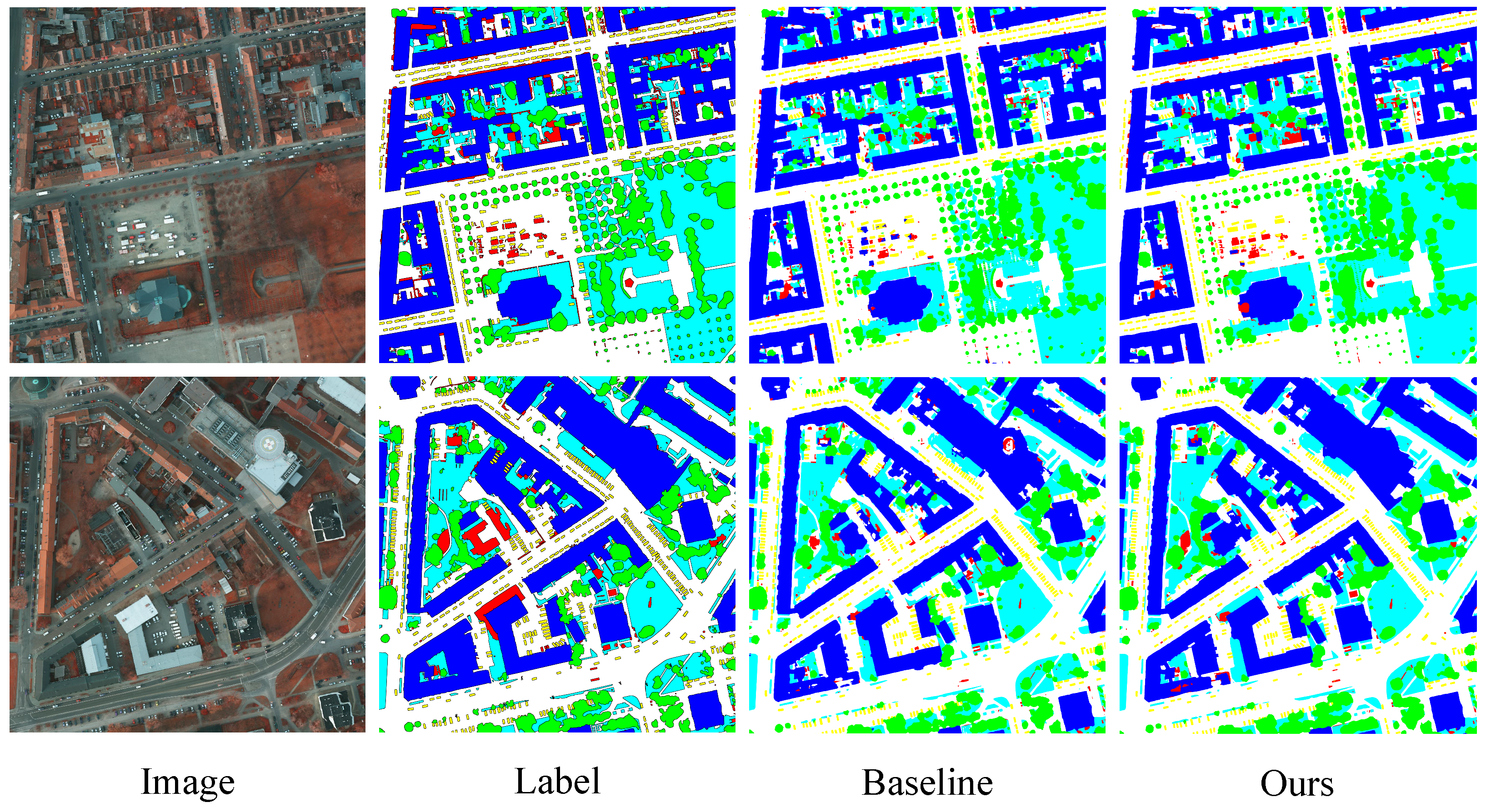
Figure 7.
Visualization of the prediction results of different methods on the Potsdam dataset. (a–e) correspond to five different input images, labels and segmentation results.
Figure 7.
Visualization of the prediction results of different methods on the Potsdam dataset. (a–e) correspond to five different input images, labels and segmentation results.

Figure 8.
Visualization of the prediction results of the proposed method and the baseline model (FCN) on the original large images of the Vaihingen dataset.
Figure 8.
Visualization of the prediction results of the proposed method and the baseline model (FCN) on the original large images of the Vaihingen dataset.

Figure 9.
Visualization of the prediction results of the proposed method and the baseline model (FCN) on the original large images of the Potsdam dataset.
Figure 9.
Visualization of the prediction results of the proposed method and the baseline model (FCN) on the original large images of the Potsdam dataset.


Table 1.
The ISPRS datasets used in this paper.
| Dataset | Vaihingen | Potsdam | ||
|---|---|---|---|---|
| Size | ||||
| GSD | 9 cm | 5 cm | ||
| Wave Bands | NIR, R, G | NIR, R, G, B | ||
| Scenes | Small Village | Large City | ||
| Train | Test | Train | Test | |
| Original Images | 16 | 17 | 24 | 14 |
| Small Patches | 705 | 398 | 7776 | 2016 |
Table 2.
Experimental setup.
| Operating System | Ubuntu 18.04.5 LTS | GPU | GeForce RTX 3090 (24 G) |
| DeepLearning Framework | Pytorch-1.7 | Batch Size | 8 |
| Training Epoch | 100 | Optimizer | SGD () |
| Vaihingen | Potsdam | ||
| Learning Rate | 0.01 | 0.005 |
Table 3.
Comparison of FCN, semantic branch, and DeepLab v3+ on Vaihingen dataset.
| Imp. Surf. | Build | Low Veg. | Tree | Car | Mean | OA | Memory Usage | |
|---|---|---|---|---|---|---|---|---|
| FCN | 91.04 | 94.19 | 81.92 | 88.13 | 79.13 | 86.88 | 88.91 | 16,980 M |
| DeepLab v3+ | 91.37 | 94.18 | 82.79 | 88.75 | 83.67 | 88.15 | 89.39 | 18,696 M |
| Semantic Branch | 92.03 | 95.11 | 83.46 | 89.10 | 82.58 | 88.46 | 90.02 | 10,005 M |
| IoU | mIoU | |||||||
| FCN | 83.56 | 89.02 | 69.38 | 78.77 | 65.47 | 77.87 | 88.91 | - |
| DeepLab v3+ | 84.12 | 89.01 | 70.63 | 79.77 | 71.93 | 79.64 | 89.39 | - |
| Semantic Branch | 85.23 | 90.68 | 71.62 | 80.35 | 70.32 | 80.34 | 90.02 | - |
Table 4.
The impact of deep supervision on semantic branch.
| Imp. Surf. | Build | Low Veg. | Tree | Car | Mean | OA | |
|---|---|---|---|---|---|---|---|
| Semantic Branch | 92.03 | 95.11 | 83.46 | 89.10 | 82.58 | 88.46 | 90.02 |
| Semantic Branch with Deep Supervision | 92.55 | 95.48 | 83.64 | 88.92 | 82.82 | 88.68 | 90.28 |
| IoU | mIoU | ||||||
| Semantic Branch | 85.23 | 90.68 | 71.62 | 80.35 | 70.32 | 80.34 | 90.02 |
| Semantic Branch with Deep Supervision | 86.12 | 91.36 | 71.88 | 80.05 | 70.67 | 80.64 | 90.28 |
Table 5.
Ablation study for the AHRM branch.
| Imp. Surf. | Build | Low Veg. | Tree | Car | Mean | OA | Memory Usage | |
|---|---|---|---|---|---|---|---|---|
| Semantic Branch | 92.55 | 95.48 | 83.64 | 88.92 | 82.82 | 88.68 | 90.28 | 10,005 M |
| + AHRM without gate | 92.32 | 95.42 | 83.85 | 89.15 | 83.41 | 88.83 | 90.32 | - |
| + AHRM with gate | 92.85 | 95.59 | 84.22 | 89.25 | 83.17 | 89.02 | 90.61 | 10,786 M |
| IoU | mIoU | |||||||
| Semantic Branch | 86.12 | 91.36 | 71.88 | 80.05 | 70.67 | 80.64 | 90.28 | - |
| + AHRM without gate | 85.73 | 91.24 | 72.19 | 80.42 | 71.54 | 80.79 | 90.32 | - |
| + AHRM with gate | 86.66 | 91.55 | 72.73 | 80.59 | 71.19 | 81.11 | 90.61 | - |
Table 6.
Ablation study for the edge branch.
| Imp. Surf. | Build | Low Veg. | Tree | Car | Mean | OA | Memory Usage | |
|---|---|---|---|---|---|---|---|---|
| Semantic Branch | 92.55 | 95.48 | 83.64 | 88.92 | 82.82 | 88.68 | 90.28 | 10,005 M |
| + edge without gate | 92.41 | 95.29 | 84.25 | 88.96 | 83.68 | 88.92 | 90.34 | - |
| + edge with gate | 92.62 | 95.43 | 84.33 | 89.28 | 84.11 | 89.15 | 90.56 | 11,190 M |
| IoU | mIoU | |||||||
| Semantic Branch | 86.12 | 91.36 | 71.88 | 80.05 | 70.67 | 80.64 | 90.28 | - |
| + edge without gate | 85.89 | 91.00 | 72.79 | 80.12 | 71.94 | 80.91 | 90.34 | - |
| + edge with gate | 86.26 | 91.26 | 72.90 | 80.63 | 72.58 | 81.22 | 90.56 | - |
Table 7.
Ablation study for weight parameter .
| Imp. Surf. | Build | Low Veg. | Tree | Car | Mean | OA | |
|---|---|---|---|---|---|---|---|
| 92.40 | 95.37 | 83.31 | 88.93 | 82.16 | 88.43 | 90.18 | |
| 92.57 | 95.39 | 84.66 | 89.32 | 83.03 | 89.00 | 90.59 | |
| 92.81 | 95.56 | 84.49 | 89.37 | 82.78 | 89.00 | 90.70 | |
| 93.02 | 95.63 | 84.74 | 89.38 | 84.58 | 89.47 | 90.82 | |
| 92.65 | 95.40 | 84.14 | 89.24 | 84.60 | 89.20 | 90.50 | |
| 92.69 | 95.46 | 83.75 | 89.14 | 84.42 | 89.09 | 90.44 | |
| 92.71 | 95.35 | 83.60 | 88.86 | 82.93 | 88.69 | 90.31 | |
| 89.94 | 92.72 | 82.07 | 88.08 | 63.73 | 83.31 | 88.11 | |
| IoU | mIoU | ||||||
| 85.87 | 91.14 | 71.40 | 80.07 | 69.72 | 80.16 | 90.18 | |
| 86.17 | 91.18 | 73.41 | 80.71 | 70.98 | 80.97 | 90.59 | |
| 86.57 | 91.50 | 73.15 | 80.79 | 70.62 | 81.02 | 90.70 | |
| 86.95 | 91.62 | 73.53 | 80.81 | 73.28 | 81.81 | 90.82 | |
| 86.30 | 91.20 | 72.62 | 80.56 | 73.31 | 81.35 | 90.50 | |
| 86.38 | 91.31 | 72.04 | 80.41 | 73.05 | 81.18 | 90.44 | |
| 86.41 | 91.11 | 71.83 | 79.95 | 70.84 | 80.65 | 90.31 | |
| 81.72 | 86.43 | 69.60 | 78.69 | 46.77 | 73.76 | 88.11 |
Table 8.
Experimental results of the final model and memory usage on Vaihingen dataset.
| Imp. Surf. | Build | Low Veg. | Tree | Car | Mean | OA | Memory Usage | |
|---|---|---|---|---|---|---|---|---|
| FCN | 91.04 | 94.19 | 81.92 | 88.13 | 79.13 | 86.88 | 88.91 | 16,980 M |
| Semantic Branch | 92.55 | 95.48 | 83.64 | 88.92 | 82.82 | 88.68 | 90.28 | 10,005 M |
| + AHRM | 92.85 | 95.59 | 84.22 | 89.25 | 83.17 | 89.02 | 90.61 | 10,786 M |
| + edge | 92.62 | 95.43 | 84.33 | 89.28 | 84.11 | 89.15 | 90.56 | 11,190 M |
| MBANet | 93.02 | 95.63 | 84.74 | 89.38 | 84.58 | 89.47 | 90.82 | 11,592 M |
| IoU | mIoU | |||||||
| FCN | 83.56 | 89.02 | 69.38 | 78.77 | 65.47 | 77.87 | 88.91 | - |
| Semantic Branch | 86.12 | 91.36 | 71.88 | 80.05 | 70.67 | 80.64 | 90.28 | - |
| + AHRM | 86.66 | 91.55 | 72.73 | 80.59 | 71.19 | 81.11 | 90.61 | - |
| + edge | 86.26 | 91.26 | 72.90 | 80.63 | 72.58 | 81.22 | 90.56 | - |
| MBANet | 86.95 | 91.62 | 73.53 | 80.81 | 73.28 | 81.81 | 90.82 | - |
Table 9.
Experimental results of the final model on the Potsdam dataset.
| Imp. Surf. | Build | Low Veg. | Tree | Car | Mean | OA | ||
|---|---|---|---|---|---|---|---|---|
| Baseline | 92.25 | 95.67 | 85.94 | 87.37 | 94.08 | 57.40 | 85.45 | 89.73 |
| MBANet | 93.20 | 96.78 | 87.12 | 88.36 | 95.64 | 61.78 | 87.15 | 90.87 |
| IoU | mIoU | |||||||
| Baseline | 85.61 | 91.71 | 75.35 | 77.57 | 88.82 | 40.25 | 76.55 | 89.73 |
| MBANet | 87.26 | 93.76 | 77.18 | 79.15 | 91.65 | 44.69 | 78.95 | 90.87 |
Table 10.
Performance of different testing methods on the Vaihingen dataset.
| SW | MS | Flip | Imp. Surf. | Build | Low Veg. | Tree | Car | Mean | OA | |
|---|---|---|---|---|---|---|---|---|---|---|
| Base | 93.02 | 95.63 | 84.74 | 89.38 | 84.58 | 89.47 | 90.82 | |||
| SW | ✓ | 93.26 | 95.74 | 85.01 | 89.91 | 86.34 | 90.05 | 91.18 | ||
| SW + MS | ✓ | ✓ | 93.56 | 96.02 | 85.75 | 90.34 | 87.95 | 90.72 | 91.59 | |
| SW + Flip | ✓ | ✓ | 93.44 | 95.95 | 85.60 | 90.43 | 87.63 | 90.61 | 91.53 | |
| SW + MS + Flip | ✓ | ✓ | ✓ | 93.60 | 96.14 | 86.19 | 90.77 | 88.33 | 91.01 | 91.82 |
| IoU | mIoU | |||||||||
| Base | 86.95 | 91.62 | 73.53 | 80.81 | 73.28 | 81.81 | 90.82 | |||
| SW | ✓ | 87.37 | 91.83 | 73.93 | 81.67 | 75.97 | 82.15 | 91.18 | ||
| SW + MS | ✓ | ✓ | 87.89 | 92.35 | 75.05 | 82.39 | 78.49 | 83.24 | 91.59 | |
| SW + Flip | ✓ | ✓ | 87.68 | 92.21 | 74.82 | 82.53 | 77.98 | 83.04 | 91.53 | |
| SW + MS + Flip | ✓ | ✓ | ✓ | 87.97 | 92.56 | 75.73 | 83.10 | 79.10 | 83.69 | 91.82 |
Table 11.
Performance of different testing methods on the Potsdam dataset.
| SW | MS | Flip | Imp. Surf. | Build | Low Veg. | Tree | Car | Mean | OA | ||
|---|---|---|---|---|---|---|---|---|---|---|---|
| Base | 93.20 | 96.78 | 87.12 | 88.36 | 95.64 | 61.78 | 87.15 | 90.87 | |||
| SW | ✓ | 93.57 | 96.97 | 87.72 | 89.00 | 95.88 | 62.87 | 92.63 | 91.31 | ||
| SW + MS | ✓ | ✓ | 93.83 | 97.15 | 88.15 | 89.16 | 96.30 | 64.19 | 92.92 | 91.62 | |
| SW + Flip | ✓ | ✓ | 93.92 | 97.16 | 88.40 | 89.48 | 96.31 | 64.24 | 93.06 | 91.75 | |
| SW + MS + Flip | ✓ | ✓ | ✓ | 94.04 | 97.23 | 88.65 | 89.57 | 96.63 | 64.77 | 93.22 | 91.90 |
| IoU | mIoU | ||||||||||
| Base | 87.26 | 93.76 | 77.18 | 79.15 | 91.65 | 44.69 | 78.95 | 90.87 | |||
| SW | ✓ | 87.92 | 94.12 | 78.12 | 80.18 | 92.09 | 45.85 | 86.49 | 91.31 | ||
| SW + MS | ✓ | ✓ | 88.38 | 94.45 | 78.82 | 80.45 | 92.87 | 47.27 | 86.99 | 91.62 | |
| SW + Flip | ✓ | ✓ | 88.54 | 94.48 | 79.22 | 80.97 | 92.88 | 47.32 | 87.22 | 91.75 | |
| SW + MS + Flip | ✓ | ✓ | ✓ | 88.76 | 94.60 | 79.61 | 81.1 | 93.48 | 47.89 | 87.51 | 91.90 |
Table 12.
Comparisons with SOTA methods on Vaihingen dataset.
| Method | Imp. Surf. | Build | Low Veg. | Tree | Car | Mean | mIoU | OA |
|---|---|---|---|---|---|---|---|---|
| UZ_1 [51] | 89.2 | 92.5 | 81.6 | 86.9 | 57.3 | 81.5 | - | 87.3 |
| RoteEqNet [52] | 89.5 | 94.8 | 77.5 | 86.5 | 72.6 | 84.2 | - | 87.5 |
| S-RA-FCN [53] | 91.5 | 95.0 | 80.6 | 88.6 | 87.1 | 88.5 | 79.8 | 89.2 |
| U-FMG-4 [54] | 91.1 | 94.5 | 82.9 | 88.8 | 81.3 | 87.7 | - | 89.4 |
| V-FuseNet [55] | 92.0 | 94.4 | 84.5 | 89.9 | 86.3 | 89.4 | - | 90.0 |
| DLR_9 [56] | 92.4 | 95.2 | 83.9 | 89.9 | 81.2 | 88.5 | - | 90.3 |
| TreeUNet [57] | 92.5 | 94.9 | 83.6 | 89.6 | 85.9 | 89.3 | - | 90.4 |
| DANet [58] | 91.6 | 95.0 | 83.3 | 88.9 | 87.2 | 89.2 | 81.3 | 90.4 |
| PSPNet [30] | 92.8 | 95.5 | 84.5 | 89.9 | 88.6 | 90.3 | 82.6 | 90.9 |
| ACFNet [59] | 92.9 | 95.3 | 84.5 | 90.1 | 88.6 | 90.3 | 82.7 | 90.9 |
| BKHN11 | 92.9 | 96.0 | 84.6 | 89.9 | 88.6 | 90.4 | - | 91.0 |
| CASIA2 [60] | 93.2 | 96.0 | 84.7 | 89.9 | 86.7 | 90.1 | - | 91.1 |
| CCNet [61] | 93.3 | 95.5 | 85.1 | 90.3 | 88.7 | 90.6 | 82.8 | 91.1 |
| BES-Net [22] | 93.0 | 96.0 | 85.4 | 90.0 | 88.3 | 90.6 | - | 91.2 |
| MBANet | 93.6 | 96.1 | 86.2 | 90.8 | 88.3 | 91.0 | 83.7 | 91.8 |
Table 13.
Comparisons with SOTA methods on Potsdam dataset.
| Method | Imp. Surf. | Build | Low Veg. | Tree | Car | Mean | mIoU | OA |
|---|---|---|---|---|---|---|---|---|
| UZ_1 [51] | 89.3 | 95.4 | 81.8 | 80.5 | 86.5 | 86.7 | - | 85.8 |
| U-FMG-4 [54] | 90.8 | 95.6 | 84.4 | 84.3 | 92.4 | 89.5 | - | 87.9 |
| S-RA-FCN [53] | 91.3 | 94.7 | 86.8 | 83.5 | 94.5 | 90.2 | 82.4 | 88.6 |
| V-FuseNet [55] | 92.7 | 96.3 | 87.3 | 88.5 | 95.4 | 92.0 | - | 90.6 |
| TSMTA [62] | 92.9 | 97.1 | 87.0 | 87.3 | 95.2 | 91.9 | - | 90.6 |
| Multi-filter CNN [63] | 90.9 | 96.8 | 76.3 | 73.4 | 88.6 | 85.2 | - | 90.7 |
| TreeUNet [57] | 93.1 | 97.3 | 86.6 | 87.1 | 95.8 | 92.0 | - | 90.7 |
| CASIA3 [60] | 93.4 | 96.8 | 87.6 | 88.3 | 96.1 | 92.4 | - | 91.0 |
| PSPNet [30] | 93.4 | 97.0 | 87.8 | 88.5 | 95.4 | 92.4 | 84.9 | 91.1 |
| BKHN3 | 93.3 | 97.2 | 88.0 | 88.5 | 96.0 | 92.6 | - | 91.1 |
| AMA_1 | 93.4 | 96.8 | 87.7 | 88.8 | 96.0 | 92.5 | - | 91.2 |
| BES-Net [22] | 93.9 | 97.3 | 87.9 | 88.5 | 96.5 | 92.8 | - | 91.4 |
| CCNet [61] | 93.6 | 96.8 | 86.9 | 88.6 | 96.2 | 92.4 | 85.7 | 91.5 |
| HUSTW4 [64] | 93.6 | 97.6 | 88.5 | 88.8 | 94.6 | 92.6 | - | 91.6 |
| SWJ_2 | 94.4 | 97.4 | 87.8 | 87.6 | 94.7 | 92.4 | - | 91.7 |
| MBANet | 94.0 | 97.2 | 88.7 | 89.6 | 96.6 | 93.2 | 87.5 | 91.9 |
Table 14.
Computational complexity of different networks.
| Model | Backbone | Params. (M) | Macs (G) |
|---|---|---|---|
| FCN | ResNet50/os = 8 | 28.23 | 119.39 |
| PSPNet | ResNet50/os = 8 | 28.29 | 133.6 |
| DANet | ResNet50/os = 8 | 36.66 | 164.75 |
| DeepLab v3 | ResNet50/os = 8 | 40.23 | 166.39 |
| DeepLab v3+ | ResNet50/os = 8 | 40.35 | 182.94 |
| MBANet | ResNet50/os = 16 | 60.66 | 102.4 |
Publisher’s Note: MDPI stays neutral with regard to jurisdictional claims in published maps and institutional affiliations. |
© 2022 by the authors. Licensee MDPI, Basel, Switzerland. This article is an open access article distributed under the terms and conditions of the Creative Commons Attribution (CC BY) license (https://creativecommons.org/licenses/by/4.0/).
Share and Cite
MDPI and ACS Style
Bai, H.; Cheng, J.; Su, Y.; Wang, Q.; Han, H.; Zhang, Y. Multi-Branch Adaptive Hard Region Mining Network for Urban Scene Parsing of High-Resolution Remote-Sensing Images. Remote Sens. 2022, 14, 5527. https://doi.org/10.3390/rs14215527
AMA Style
Bai H, Cheng J, Su Y, Wang Q, Han H, Zhang Y. Multi-Branch Adaptive Hard Region Mining Network for Urban Scene Parsing of High-Resolution Remote-Sensing Images. Remote Sensing. 2022; 14(21):5527. https://doi.org/10.3390/rs14215527
Chicago/Turabian StyleBai, Haiwei, Jian Cheng, Yanzhou Su, Qi Wang, Haoran Han, and Yijie Zhang. 2022. "Multi-Branch Adaptive Hard Region Mining Network for Urban Scene Parsing of High-Resolution Remote-Sensing Images" Remote Sensing 14, no. 21: 5527. https://doi.org/10.3390/rs14215527
Note that from the first issue of 2016, this journal uses article numbers instead of page numbers. See further details here.