Feature Weighted Attention—Bidirectional Long Short Term Memory Model for Change Detection in Remote Sensing Images

Abstract

In remote sensing images, change detection (CD) is required in many applications, such as: resource management, urban expansion research, land management, and disaster assessment. Various deep learning-based methods were applied to satellite image analysis for change detection, yet many of them have limitations, including the overfitting problem. This research proposes the Feature Weighted Attention (FWA) in Bidirectional Long Short-Term Memory (BiLSTM) method to reduce the overfitting problem and increase the performance of classification in change detection applications. Additionally, data usage and accuracy in remote sensing activities, particularly CD, can be significantly improved by a large number of training models based on BiLSTM. Normalization techniques are applied to input images in order to enhance the quality and reduce the difference in pixel value. The AlexNet and VGG16 models were used to extract useful features from the normalized images. The extracted features were then applied to the FWA-BiLSTM model, to give more weight to the unique features and increase the efficiency of classification. The attention layer selects the unique features that help to distinguish the changes in the remote sensing images. From the experimental results, it was clearly shown that the proposed FWA-BiLSTM model achieved better performance in terms of precision (93.43%), recall (93.16%), and overall accuracy (99.26%), when compared with the existing Difference-enhancement Dense-attention Convolutional Neural Network (DDCNN) model.

1. Introduction

Change detection in remote sensing images is an essential part in numerous applications of remote sensing technology. The existing change detection (CD) and deep learning (DL) methods do not explicitly distinguish between areas that are changed and those that are unchanged, resulting in the loss of edge detail information during detection [1]. CD involves finding the alteration in the surface. In practical applications, change detection is performed on different resolutions of bi-temporal images. Traditionally, it is performed using a sub-pixel-based technique on images with different resolution, which often causes errors in case of high-resolution images due to interclass similarity and intraclass heterogeneity [2,3]. In the case of satellite images, CD is widely applied in, e.g.,: urban expansion research, resource management, land management, and disaster assessment. Traditional change detection methods use threshold segmentation or clustering techniques to process various images in order to find unaltered or modified regions [4]. The exponential growth of computing power and strong capacity of representation learning helps to apply deep convolutional neural networks (CNNs) in this area of research [5].

Automatic change detection in remote sensing images is important for various applications, such as mapping of land use. Recently, several researchers have applied DL techniques in this area. Aerial images or multi-temporal satellite images provide a variety of information, which can be utilized for detecting differences in land use or land cover in a particular region over a period of time [6]. Deep CNN models provide significant performance in change detection of satellite images. CNN models learn feature representation from input images at various resolutions from low to high [7]. High-level feature representation is automatically learned using CNN models and provides superior performance to traditional techniques on low-level features [8]. CNN models have been used in numerous fields over the past years [9,10,11,12,13,14,15,16,17] and applied in remote sensing classification. However, CNN models have an overfitting problem that affects the model’s efficiency.

The major purpose of image CD is to recognize the areas that have undergone modification between two images, taken at different periods of time in the same geographic location. Direct comparison is quite challenging, because of the varied feature maps in these images. To solve this issue, the pixel-level transformation approach is applied. Certain transformation techniques that are based on object and feature level perform poorly when it comes to detail preservation. In order to maintain more details and fully utilize the pixel information in the image, as well as to provide a more accurate change detection capability, a number of deep learning methods are implemented.

DL models have been extensively used in several fields recently Among the current DNN models considered, the Siamese network takes longer training time than other DNN networks, and is also slower than traditional classification-type learning because it utilizes quadratic pairings for learning purposes. Therefore, the Bidirectional Long Short-Term Memory (BiLSTM) method was selected for this research. The extension of conventional LSTMs, called the bi-directional LSTM, can enhance predictive accuracy on sequence classification issues. The BiLSTM differs from a standard LSTM in that the input can flow either backwards or forward. Consequently, bi-directional input maintains both future and historical knowledge by allowing input data to flow in both directions. The main objectives and contribution of this research are as follows:

• The Feature Weighted Attention (FWA) technique is applied to provide weight values to features, and is used by the BiLSTM model for classification to help focus on the most relevant characteristics for classification and reduce the overfitting problem.
• The FWA-BiLSTM model focuses on unique features that help to find changes in the input images. This helps to distinguish the alteration in an image and increases the classification performance of the FWA-BiLSTM model.
• The AlexNet and VGG16 models are used for feature extraction from normalized images and applied to the FWA-BiLSTM model for classification purposes. The FWA-BiLSTM model obtains higher efficiency than existing deep learning techniques.

This paper is organized as follows: a literature review of recent advances in change detection is presented in Section 2. An explanation of the FWA-BiLSTM model is provided in Section 3. The simulation setup is described in Section 4. The results and discussion are given in Section 5. Conclusions and future study directions can be found in Section 6.

2. Related Works

Change detection in remote sensing images is the process of identifying the alterations occurring in the same geographic area. Recently, deep learning techniques have been applied for the detection of modifications. Previously published works on this topic are summarized in

Table 1. Comparison of published works related to change detection under various approaches.

Method/ Technique	Advantage	Disadvantage
Li et al. [18]	The DTCDN model was proposed with cyclic structure to improve the performance of change detection on optical and SAR images.	The exploitation performance of the DTCDN model was low and reduced the efficiency of the model.
Wang et al. [19]	ADS-Net was established with features which were mapped into a deep supervision network to construct a change map in different branches for increased efficiency.	The overfitting problem in the deep network degraded the performance of classification.
Fang et al. [20]	The proposed SNUNet-CD was composed of deep layers on a neural network to alleviate information of localization loss using encoder and decoder.	The overfitting problem occurred in the network due to the generation of additional features.
Shi et al. [21]	The proposed DSAMNet model was applied to learn map changes in order to provide discriminative features which helped to enhance feature learning performance and generate more useful features.	The DSAMNet model had lower efficiency in measuring semantic changes in the different scenarios.
Zheng et al. [22]	The proposed CLNet was based on UNet structure and Cross Layer Blocks which considered multi-scale features and multi-level context information to improve the performance of the CD model.	The CLNet model required a larger number of training images and had an overfitting problem.
Chen et al. [23]	The proposed Bi-temporal Image Transformer (BIT) method was based on ResNet18 and UNet models which helped to achieve higher performance in classification.	The overfitting problem occurred in the network and degraded the classification performance.
Peng et al. [24]	The proposed UNet++ used a semantic segmentation and an encoder–decoder architecture to provide feature maps with high spatial accuracy.	The overfitting problem occurred in the network due to the generation of multiple features needed for classification.
Zhang et al. [25]	A deep model of Image Fusion Network (IFN) used the architecture of a two-stream fully convolutional model to improve the performance of CD in satellite images.	The DDN model had lower efficiency in handling semantic features and reduced the efficiency of the model.
Chen et al. [26]	The DAFCSN extracted long-range dependencies of more discriminant feature representations to enhance the performance of model recognition.	The DAFCSN required more training data and the overfitting problem reduced the model performance.
Jiang et al. [27]	This PGA-SiamNet provided correlation among input feature pairs to improve various attention techniques and feature aggregation.	The PGA-SiamNet model limitation was the overfitting problem that degraded the performance of classification.
Li et al. [28]	In MFCN, loss function and dice coefficient loss were applied to train imbalanced datasets for improving the CD efficiency.	The developed model required more training images for classification and had an overfitting problem.
Peng et al. [29]	The high-level features from the DDCNN were selected and its spatial context information was used to change the features which improve the overall accuracy.	The end-to-end model had lower efficiency in imbalanced datasets and the overfitting problem affected the classification.

.

Li et al. [18] applied a deep CNN based model named DTCDN to improve the performance of CD in the case of optical and SAR images. The cyclic structure of the same feature space was used in deep translation to map from the optical to the SAR domain. The exploitation performance of the model was low and reduced the efficiency of the model.

Wang et al. [19] applied the attention technique based on deep supervision network (ADS-Net) to increase the efficiency of the change detection model. A full convolutional network with encoding–decoding was designed using a dual stream structure. In the encoding stage, multiple features were extracted, and in the decoding stage, various levels of features were mapped into a deep supervision network to construct a change map in different branches. The overfitting problem in the deep network degraded the performance of classification.

Fang et al. [20] applied the Siamese network for change detection, named SNUNet-CD. SNUNet-CD was composed of deep layers on a neural network to alleviate information of localization loss using an encoder and decoder. Deep supervision of the Ensemble Channel Attention Module (ECAM) and different semantic levels of the most representative features were refined in the final classification. The overfitting problem occurred in the network due to the generation of too large a number of features.

Shi et al. [21] applied the attention technique in a deep model named DSAMNet, utilized for change detection in satellite images. The DSAMNet model was applied to learn map alterations using deep metric learning to provide discriminative features using convolutional block attention modules. Deep learning technology helped to enhance feature learning performance and generate more useful characteristics. The model had lower efficiency in measuring semantic changes in different scenarios.

Zheng et al. [22] applied the Cross Layer CNN (CLNet) model to improve the performance of the change detection model. The CLNet was based on the UNet structure and Cross Layer Blocks (CLBs) to consider multi-scale features and multi-level context information. The CLB was applied with one input with two parallel but asymmetric branches, which were split in order to extract multi-scale features. The CLNet model required a large number of training images and had an overfitting problem as well.

Chen et al. [23] applied a Bi-temporal Image Transformer (BIT) method for the extraction of effective features in the spatial–temporal domain. A few visual words of semantic tokens were used to represent a change of interest in high-level concepts. A few tokens were used to express a bi-temporal image and apply a transformer encoder to compact token-based space–time in the model context. The pixel space was used for feedback on learned context-rich tokens for refining original features using a transformer decoder. The developed model was based on the ResNet18 and UNet model, which helped to achieve high performance in classification. The overfitting problem occurred in the network and degraded the classification performance.

Peng et al. [24] applied an end-to-end change detection technique using semantic segmentation and an encoder–decoder architecture named UNet++ to change maps learned from scratch. The co-registered image pairs were used by the improved UNet++ network to focus on fine-grained and global information thereby providing feature maps of high spatial accuracy. The fusion technique of multiple side outputs was applied to combine various semantic levels of change maps in order to develop a final change map. The overfitting problem occurred in the network due to the generation of many features required for classification.

Zhang et al. [25] applied a deep model of Image Fusion Network (IFN) to improve the performance of change detection in satellite images. Deep features were extracted using the architecture of a two-stream fully-convolutional model. The Difference Discrimination Network (DDN) of the supervised model was applied with extracted features for change detection. The DDN model had lower efficiency in handling semantic features which reduced the efficiency of the model.

Chen et al. [26] applied a deep CNN-based model named DAFCSN for change detection in satellite images. The dual attention technique extracted long-range dependencies of more discriminant feature representations to enhance the performance of model recognition. Change detection model performance was affected by the imbalanced samples and pseudo change effects. The developed method required more training data and the overfitting problem reduced the model performance once again.

Jiang et al. [27] applied a Siamese network-based model named PGA-SiamNet to an end-to-end network for change detection. This analysed the degree of correlation between pairs of input feature using the global co-attention technique. Long-range dependencies of the features were used to improve various attention techniques and to aggregate feature co-attention levels. The overfitting problem was the limitation of the PGA-SiamNet model that degraded its performance in classification.

Li et al. [28] applied a deep CNN based model for change detection in satellite images. The imbalance problem affected the efficiency of change detection. The Multi-Scale Fully CNN (MFCN) model was applied to utilize multi-scale convolution kernels to extract ground object features. Weighted Binary Cross-Entropy (WBCE) using loss function and dice coefficient loss was applied in the model to train imbalanced datasets. The developed model required many training images for classification and, once again, suffered from the overfitting problem.

Peng et al. [29] applied an end-to-end change detection network called Difference-enhancement Dense-attention Convolutional Neural Network (DDCNN) model. An up-sampling attention unit of a dense attention model was used to model the internal correlation between low-level and high-level features. The unit adopted both up-sampling channel attention and sampling spatial attention. The high-level features with rich category information were selected and spatial context information was used to change the features of the ground object. The end-to-end model had lower efficiency in imbalanced datasets and the overfitting problem was present once again.

According to available literature, many difficulties have developed as a result of advances in image technology and various sensor characteristics. First, the spatial and spectral quality of remote sensing images continue to advance, as a wealth of ground object data is made available, drastically increasing noise and redundancy. Next, a wider range of domains are regularly included in the applications of remote images. Therefore, the majority of difficult tasks can no longer be done by a single model. Many studies in the area of feature extraction are currently being conducted using deep learning techniques. Thus, research into DL-based remote sensing image CD technologies offers a new automatic and intelligent processing approach in addition to improving accuracy to meet the needs of modern-day information, communication, and technology (ICT) applications.

3. Proposed Method

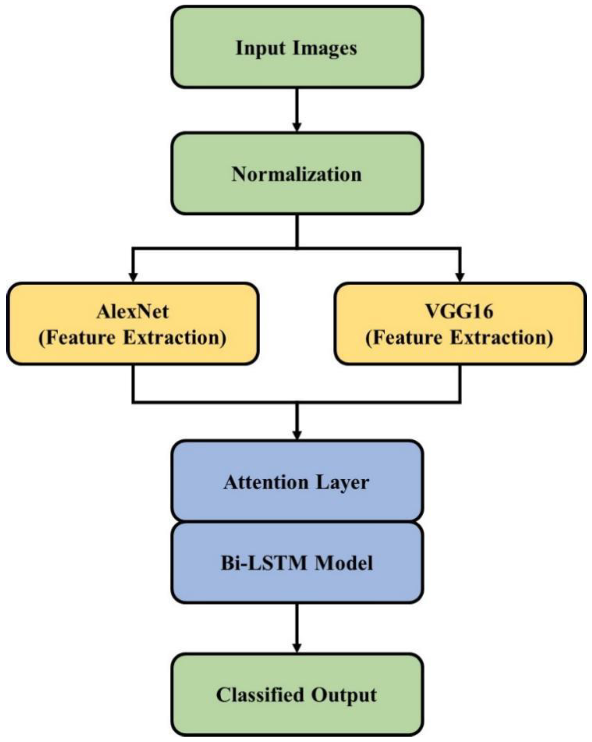
The remote sensing images underwent a normalization process in order to improve image quality. The AlexNet and VGG16 models were utilized to input images for extracting deep features. The extracted features were applied to FWA-BiLSTM for classification of change detection. The overview of the FWA-BiLSTM model in CD is shown in Figure 1.

3.1. Min–Max Normalization

The min–max normalization technique was applied to reduce the difference between pixels in the image and to improve image quality. The formula for min–max normalization is given in Equations (1) and (2):

$$X_{std}=\frac{X-X_{min}}{X_{max}-X_{min}}$$

(1)

$$X_{scaled}=X_{std}\times \left(max-min\right)+min$$

(2)

where the minimum feature range is $min$, and the maximum feature range is $max$.

3.2. Feature Extraction

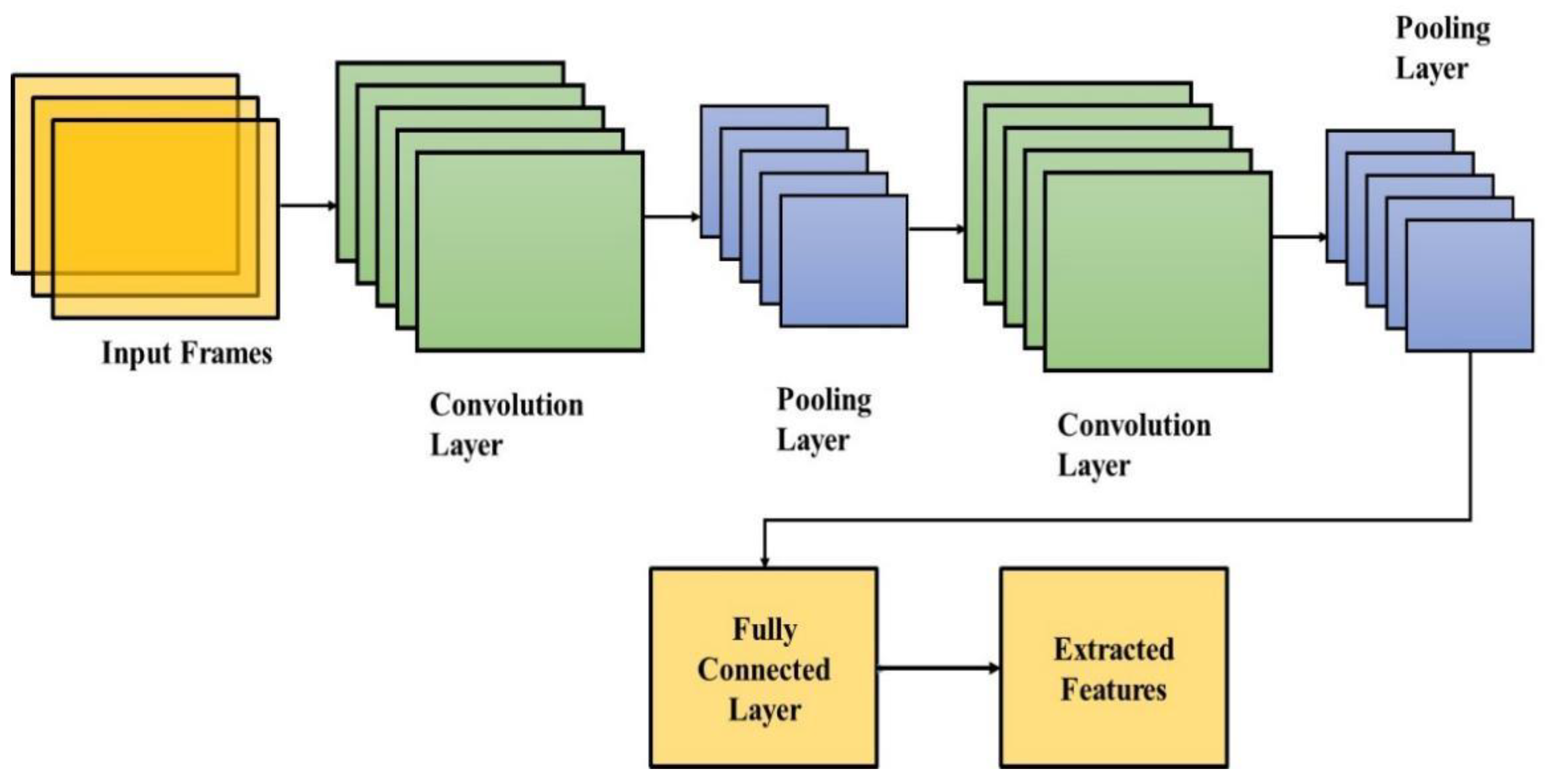
AlexNet and VGG16 models were used to extract deep features from input images. The CNN model [30] is based on an Artificial Neural Network and a convolutional layer with other layers was utilized, such as: fully connected layers, pooling, and non-linear, to develop deep CNN. CNN can be beneficial depending on the application and training parameters. In CNN, the backpropagation technique is applied with convolutional filters in training. The filter shapes are based on a given task and in change detection applications: one filter performs edge extraction and another performs CD itself. CNN filters are not fully controlled and different values are selected through learning.

Convolutional Layer: In the convolutional layer, kernel filters are applied in the input data layer. Multiplication summation of the filters, element by element, is applied and layer output calculates the input receptive field. The next layer element of weighted summation is provided and the focused area is used to multiply the filter matrix. The focus center has corresponding multiplication results that are given in the next layer. The focus area is a slide and replaces the convolution result of other elements.

Zero padding, filter size, and stride: These are used to specify each convolutional operation. Stride is used to measure the sliding step based on a positive integer number. For instance, Stride 1 denotes each time a filter is slid one place to the right and the output is calculated. Zero padding applies zeros to rows and columns to control feature map size in the original input matrix. In the same convolutional operation, the receptive field or filter size is fixed.

Non-Linearity: The main purpose of non-linearity is a cut-off to generated output, and CNN uses several non-linear functions. The Rectified Linear Unit (ReLU) is a common non-linearity in various fields of image processing. Equation (3) represents the ReLU:

$$ReLU=\{\begin{array}{cc}0,& if x<0,\\ x,& if x\ge 0\end{array}$$

(3)

Pooling Layer: The input dimension is reduced by the pooling layer. A commonly used pooling technique is max pooling and a pooling filter (2 × 2) maximum value is used as the output. Summation and averaging are other pooling techniques. The max-pooling technique is widely used in various types of research, and due to this it has significant results in down-sampling.

Softmax Layer: A softmax layer is used to provide categorical distribution in the model. The softmax function is applied in the output layer that normalizes the output values exponent. This difference enables the function and denotes output probability. The probability maximum value is increased by raising the exponential element. Equation (4) describes the softmax formula:

$$o_i=\frac{e^{z_i}}{{\sum }_i^M{e}^{z_i}}$$

(4)

where the total number of output nodes is denoted as $M$, $z_i$ is the output $i$ before the softmax, and $o_i$ is the softmax output number $i$. The CNN architecture for feature selection is shown in Figure 2.

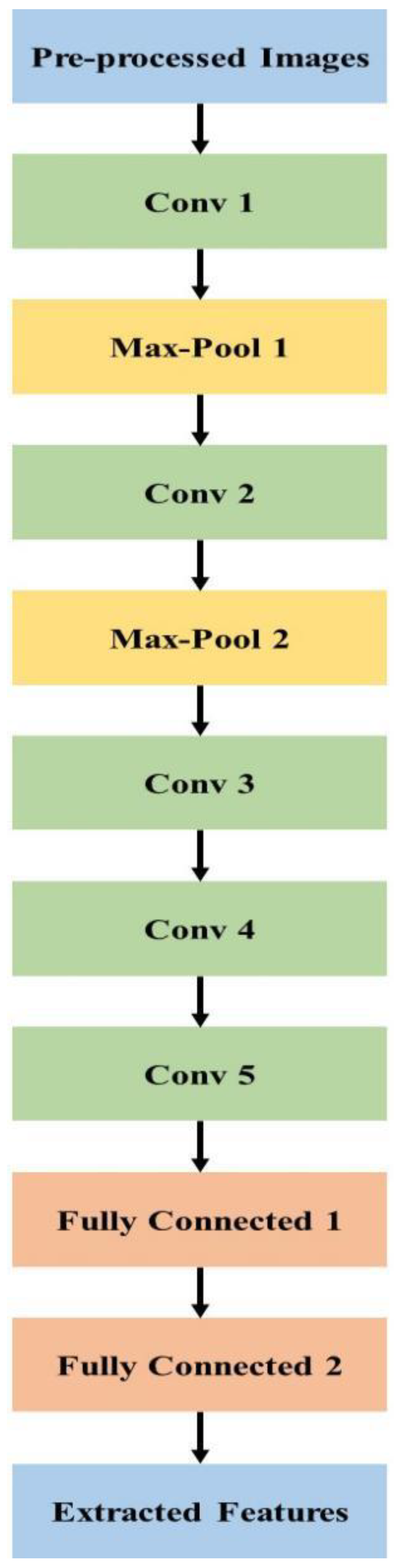
3.2.1. AlexNet Model

The AlexNet [31,32,33] model provides successful classification in various types of research, and this shows superior performance in image classification to previous methods, because it adopts an architecture with consecutive convolutional layers. Deep learning researchers show much interest in AlexNet. Additionally, AlexNet supports multi-graphical processing unit (GPU) training by splitting the model’s neurons in half and training them on different GPUs. This not only allows for the training of a larger model, but also shortens the training period.

The activation function is applied in AlexNet and the non-linearity of neural networks is given in the activation function. Conventional activation functions are arctan function, tanh function, logistic function, etc. In deep learning, these functions cause a gradient vanishing problem, and a large gradient value is provided for input in a small range around 0. The activation function of ReLU is applied to overcome this problem. Equation (5) describes the ReLU:

$$ReLU\left(x\right)=\max \left(x,0\right)$$

(5)

If the input is not less than 0, the ReLU gradient is always 1, and this proves that ReLU—as an activation function in deep networks—provides higher convergence than the tanh unit. Training causes further acceleration.

The overfitting problem is solved using the dropout layer and is applied in fully connected layers. Every iteration and dropout is used to train a part of the neurons. For instance, if the dropout is set as 50%, half of the neurons are trained and the remaining ones are skipped in subsequent iterations. Dropout improves generalization, minimizes joint adaptation of neurons, and increases cooperation between neurons. The dropout is performed on several sub-networks or segments on the network. The same loss function is shared in each single sub-network and causes an overfit to a certain extent. The entire network output is the average of sub-networks, and dropout improves the robustness.

Automatic feature extraction and reduction are carried out using pooling and convolution layers. The convolution layer is applied for signal analysis. Considering an image $M$ of size $\left(m,n\right)$, the convolution is given in Equation (6):

$$C\left(m,n\right)=\left(M\times w\right)\left(m,n\right)={\sum }_k{\sum }_{l}M\left(m-k,n-l\right)w\left(k,l\right)$$

(6)

where: convolution kernel $w$ is of size $\left(k,l\right)$. The model solution is provided by convolution to learn image features, and model complexity is reduced by parameter sharing. The pooling layer uses the feature maps in a neighboring pixel group to perform feature reduction and some value is provided for representation. The size of the feature map is $4\times 4$, and the max value in every $2\times 2$ block of max pooling generated substantially reduces the feature dimension.

Generalization is improved by cross-change normalization, which is a type of local normalization. Cross-channel normalization in neurons provides a sum of several adjacent maps at the same position. The normalized feature maps are applied to the next layers. A pixel is considered to have changed when the difference between the observed and predicted pictures exceeds a threshold three times in a row. Change detection is followed by classification.

Classification is performed using fully connected layers, and neurons are fully connected to adjacent layers. The softmax activation function is used in these layers, as given in Equation (4).

Softmax constrains the range of (0, 1) output, and ensures neuron activation. In AlexNet training, other techniques are used, such as training on multiple Graphical Processing Units (GPUs), and overlapping pooling. The AlexNet architecture for feature selection is shown in Figure 3.

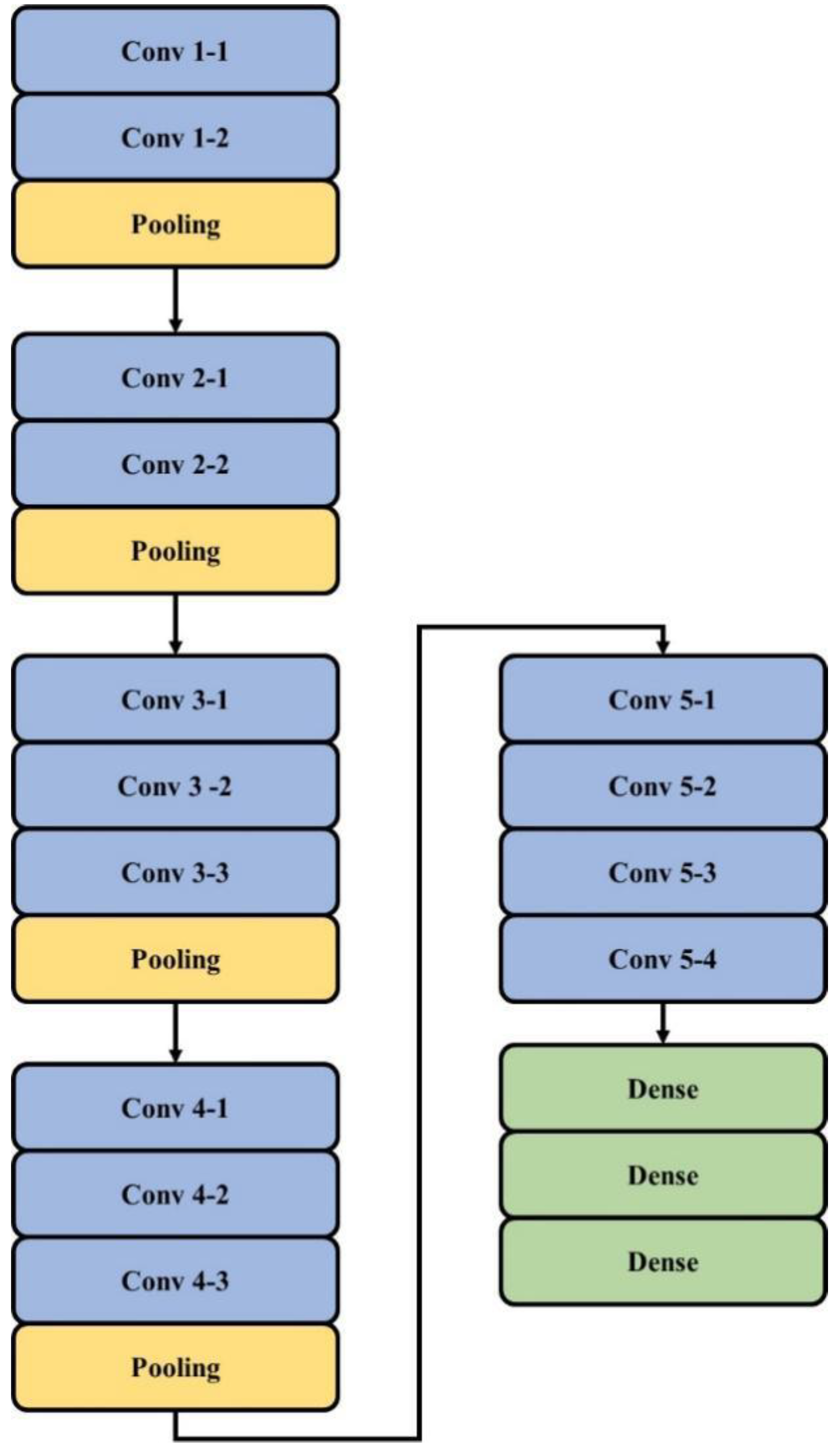
3.2.2. VGG16 Model

The VGG16 architecture model consists of 10 identical deep neural structures that are derived from the VGG16 model and MLP network [34,35,36]. The VGG16 algorithm for object recognition and classification can accurately classify more images from different classes. It is a popular technique for classifying images and is simple to employ with transfer learning. Figure 4 shows a deep neural network for each 10 identical and original VGG 16 models, which is applied with convolution blocks, i.e., the weight and bias of the VGG16 model is preserved by deleting the VGG16 fully connected layer. The deep neural structure outputs are applied to MLP input to construct a classification network.

The two layers of MLP networks of the fully connected layer are constructed that apply the loss function, as given in Equation (7):

$$Loss=\frac{1}{m}{\sum }_{i=1}^m\left[-\left({\alpha }_1{y}^i\log \left({\widehat{y}}^i\right)+{\alpha }_2\left(1-y^i\right)\log \left(1-{\widehat{y}}^i\right)\right)\right]$$

(7)

where: batch size is denoted as $m$, and a binary indicator is defined as $y^i$ (0 or 1). The order is denoted with 0 and the disorder is denoted with 1. The output is $y^i=1$ and predicted probability is denoted as ${\widehat{y}}^i$. Similarly, the predicted probability of $y^i=0$ is denoted as $1-{\widehat{y}}^i$. The weight computation parameters are ${\alpha }_1$ and ${\alpha }_2$.

3.3. BiLSTM Model

The obtained output from the AlexNet and VGG16 are given to the attention layer, where different weight values are applied in the attention model to focus on important features in the input features. The weight of the significant features in the convolutional transformation part is increased by using the attention models. The mean value and the maximum value of the defining images are the two components that make up the weight calculation for the attention mechanism in the system. The weight value reflects the aspects of the images which are critical for classification of features, allowing the model to learn to extract critical image parameters in the testing set. The attention mechanism optimizes the feature maps in the network during the training phase. Consequently, the extracted features of AlexNet and VGG16 are combined to improve image classification effectiveness. The hidden states $S_{A_W}$ of a weighted combination helps to apply different weights to different features, as described in Equations (8) and (9).

$${\alpha }_t=\frac{\exp \left(v^T.\tilde{h}\right)}{{\sum }_t\exp \left(v.\tilde{h}\right)}$$

(8)

$$S_{A_W}=\sum _t{\alpha }_t{h}_t$$

(9)

The BiLSTM trainable parameter is denoted as $v$, and the hidden layer is denoted as $\tilde{h}$ and $h$. The BiLSTM formula is denoted as follows:

$$i_t=\sigma \left(W_i\left(\left[x_t,y_{t-1}\right]\right)\right)$$

(10)

$$f_t=\sigma \left(W_f\left(\left[x_t,y_{t-1}\right]\right)\right)$$

(11)

$$o_t=\sigma \left(W_0\left[\left(x_t,y_{t-1}\right)\right]\right)$$

(12)

$$g_t=\tan \mathrm{h}\left(W_g\left(\left[x_t,y_{t-1}\right]\right)\right)$$

(13)

$$c_t=f\odot c_{t-1}+i\odot g$$

(14)

$$y_t=o\odot \tan \mathrm{h}\left(c_t\right)$$

(15)

where: input modulation, output, forget, and input gate are denoted as $c$, $g$, $o$, $f$, and $i$, respectively. The sigmoid function is denoted as $\sigma$ in Equations (10)–(13), and the weight value of a fully connected neural network for input modulation, output, forget, and input gate are denoted as $W_g$, $W_o$, $W_f$, and $W_i$, respectively. The element-wise product operator is denoted as $\odot$ in Equations (14) and (15). The LSTM model considers a sequence of one-directional information that reduces its effectiveness. Valuable information is retrained using bi-directional information of a sequence. The BiLSTM model is a combination of forward and backward direction in a sequence [37,38]. Forward processing is carried out by LSTM layers and backward processing is carried out by the remaining layers.

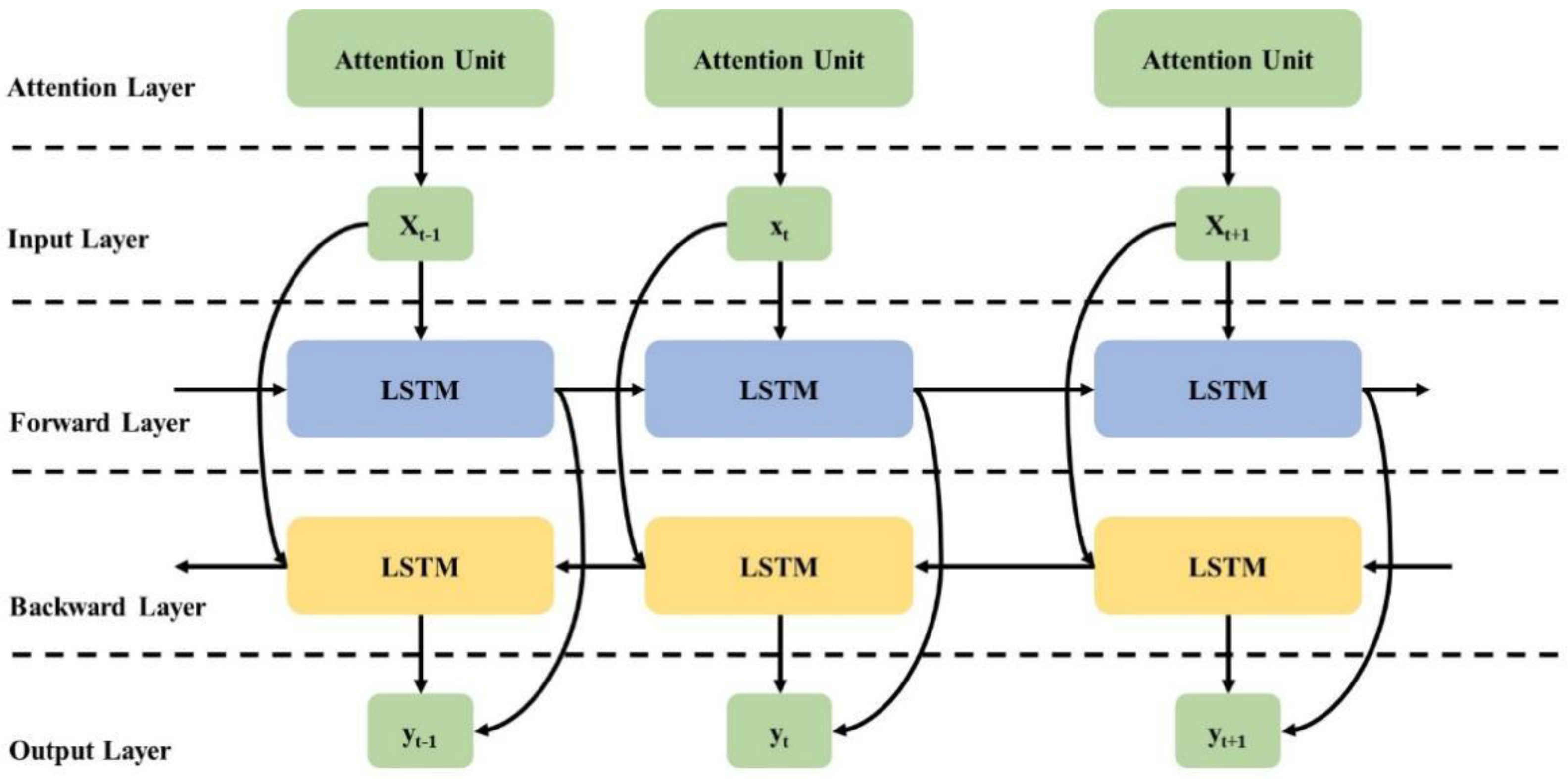
Consider $x$ input sequence with $n$ elements. The LSTM forward order is $\left\{x_1,x_2,...,x_n\right\}$ and LSTM backward is $\left\{x_n,x_{n-1},...,x_1\right\}$. LSTM forward and backward separation is performed and outputs are fused in LSTMs to integrate into the previous step, denoted in Equation (16):

$$y\left(t\right)=y_F\left(t\right)\oplus y_B\left(n-t+1\right)$$

(16)

where forward and backward LSTMs outputs are denoted as $y_F$ and $y_B$, respectively. A simple neural network adder is included using an integration operator. Equation (16) combines the forward and backward directions of the BiLSTM model. Two fully connected layers of BiLSTM outputs are applied to generate values of energy consumption. The Attention Unit with the BiLSTM model is shown in Figure 5.

4. Simulation Setup

Designed for change detection, the FWA-BiLSTM model is discussed in this section, and its simulation setup details considered.

Datasets: The LEVIR-CD [39] has 637 images of a pixel size of $1024\times 1024$. The images are collected in 20 different regions of Texas in the U.S. over a period of 5–14 years. The season varying dataset [40] images are of a pixel size of $4725\times 2700$ in 7 pairs of co-registered images from Google Earth. Bi-temporal images with season changes are included in the dataset.

Metrics: Precision, Recall, F1-Score, and Overall Accuracy formulas are given in Equations (17)–(20).

$$Precision(\%)=\frac{TP}{TP+FP}\times 100$$

(17)

$$Recall(\%)=\frac{TP}{TP+FN}\times 100$$

(18)

$$F1-Score(\%)=\frac{2TP}{2TP+FP+FN}\times 100$$

(19)

$$Overall Accuracy(\%)=\frac{TP+TN}{TP+TN+FP+FN}\times 100$$

(20)

Parameter Settings: The parameter settings for AlexNet, VGG16, and BiLSTM are 8 epochs, 0.1 dropout rate, 0.01 learning rate, and Adam optimizer.

System Requirement: The FWA-BiLSTM model is implemented on a computer running the Windows 10 OS, with a 6 GB graphics card, 16 GB of RAM, and an Intel i-7 processor.

5. Results

The FWA-BiLSTM model was tested on two datasets, namely, LEVIR-CD and SVD, to evaluate its performance. The classifiers, including CNN, LSTM, and Siamese Neural Network (SNN) [41], were used to compare the obtained results with the FWA-BiLSTM model.

5.1. Quantitative Analysis on LEVIR-CD Dataset

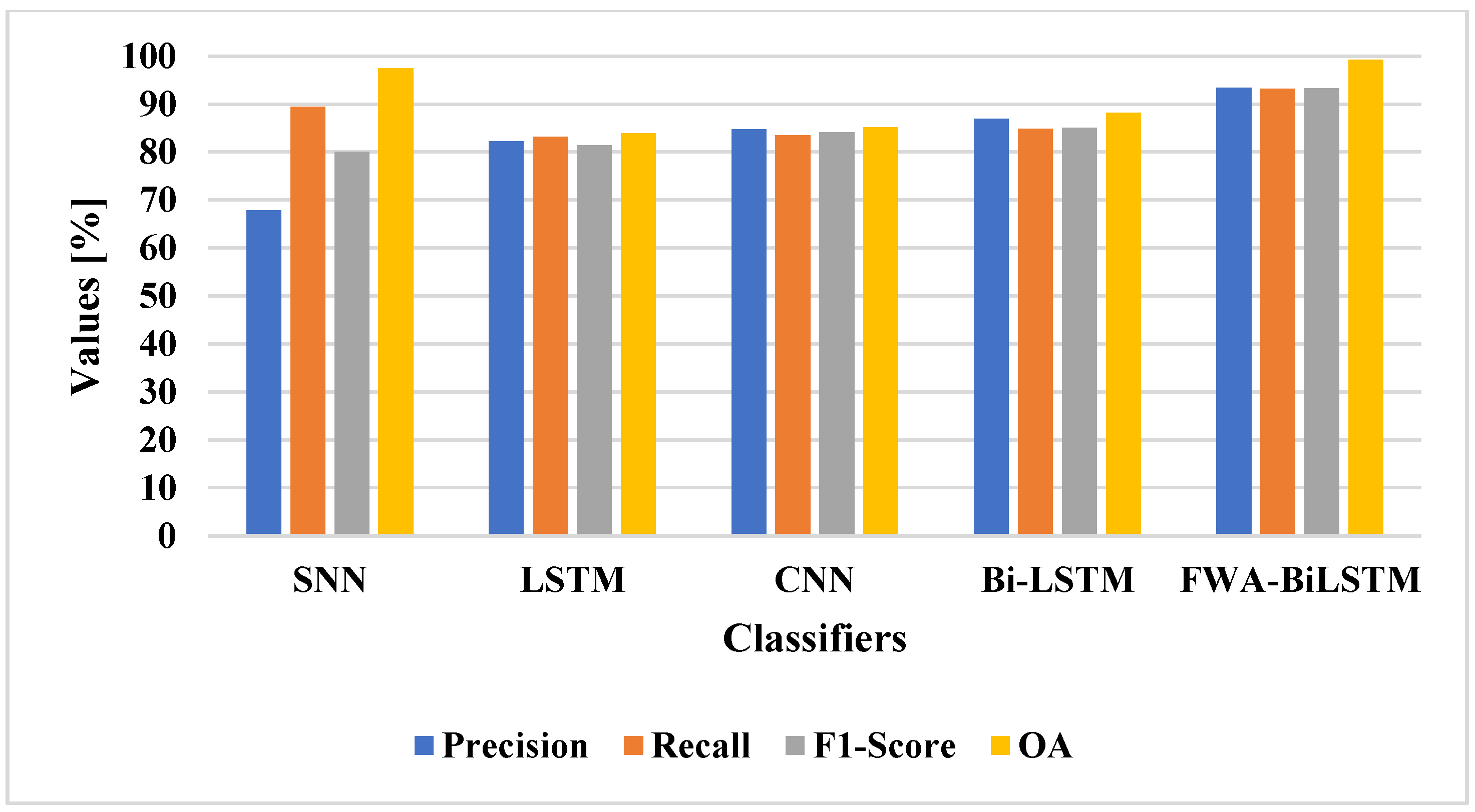
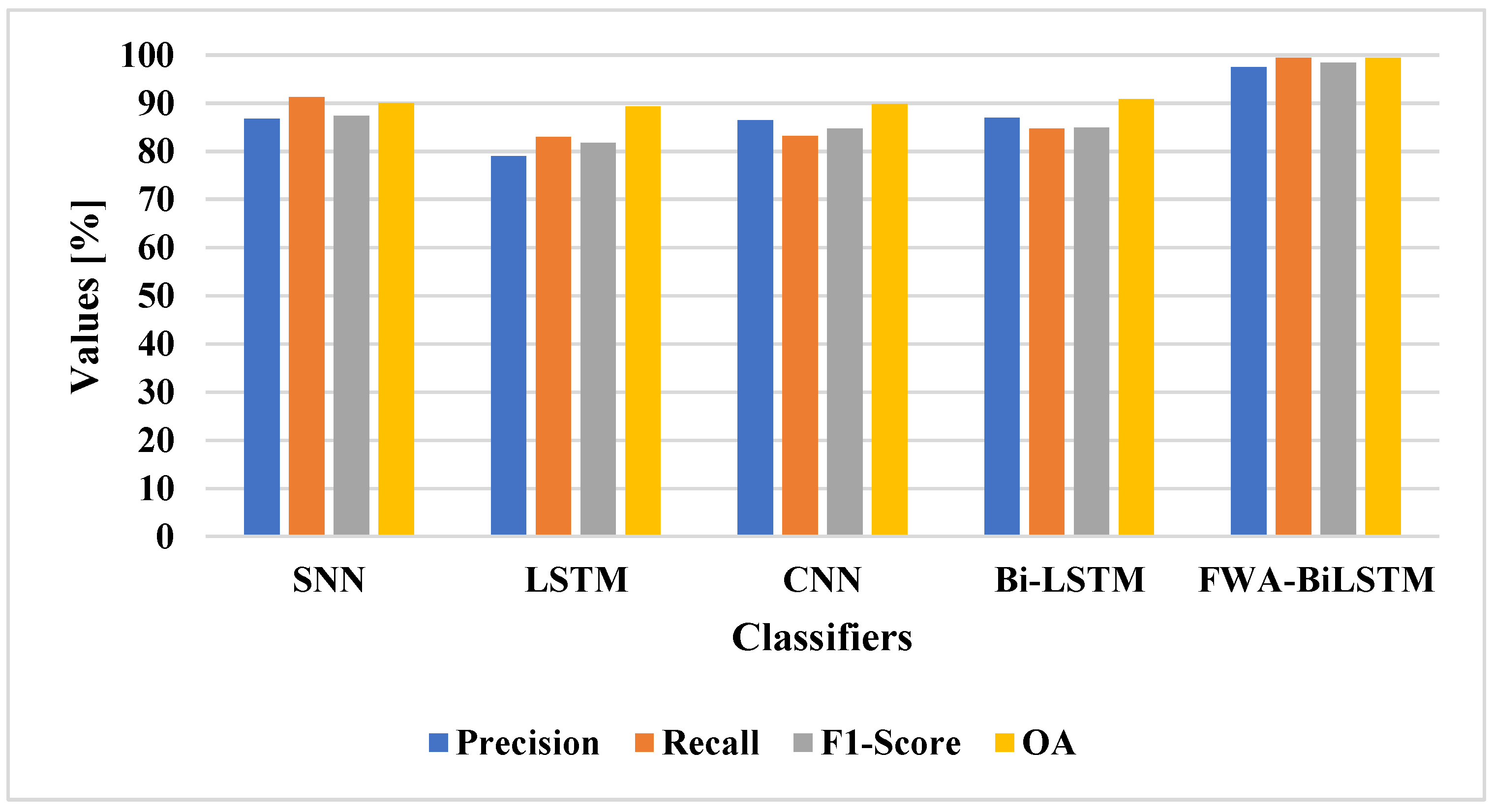
The FWA-BiLSTM model was tested on the LEVIR-CD dataset and compared with deep learning techniques. The FWA-BiLSTM model was compared with classifiers on the LEVIR-CD dataset, as shown in

Table 2. Performance analysis of classifiers without attention layer on LEVIR-CD dataset.

Methods	Precision [%]	Recall [%]	F1-Score [%]	OA [%]
SNN	67.87	89.48	80.04	97.52
LSTM	82.19	83.21	81.41	83.89
CNN	84.72	83.53	84.12	85.17
BiLSTM	86.91	84.80	85.01	88.18
FWA-BiLSTM	93.43	93.16	93.29	99.26

and Figure 6. The performance and reliability of the proposed method need to be demonstrated for CD utilizing quantitative analysis. Outcomes from CDs are typically displayed as binary images for performance assessment, where white pixels represent altered pixels and black pixels denote unchanged pixels. In this research, the proposed approaches were evaluated using a set of factors, namely: precision, recall, F1-score, and OA.

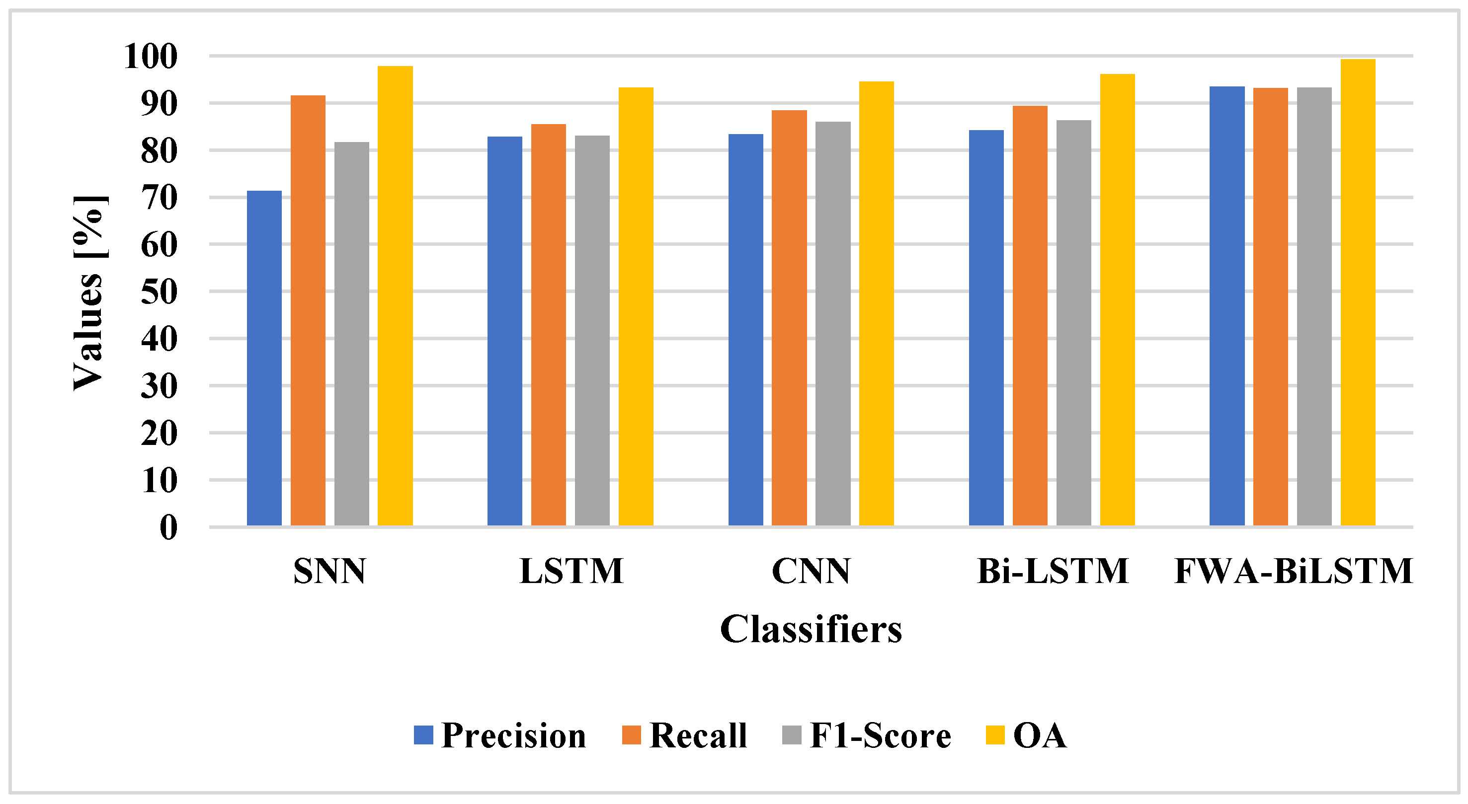
The FWA-BiLSTM model had an attention layer that provided higher feature weight values to relevant features which helped the BiLSTM model to increase the efficiency of the classification. The SNN [41] obtained better performance in an imbalanced dataset, while the LSTM and BiLSTM models had vanishing gradient problems, and the CNN model encountered an overfitting problem. When compared with existing methods, the proposed FWA-BiLSTM model achieved a higher recall value. Due to this fact, the model selected unique features in order to distinguish the changes. The FWA-BiLSTM model obtained 93.43% precision, 93.16% recall, and 99.26% OA, whereas the BiLSTM model had 86.91% precision, 84.80% recall, and 88.18 %OA. The FWA-BiLSTM was compared with attention layer classifiers on the LEVIR-CD dataset, as shown in

Table 3. Performance of classifier with attention layer on LEVIR-CD dataset.

Methods	Precision [%]	Recall [%]	F1-Score [%]	OA [%]
SNN	71.37	91.53	81.66	97.82
LSTM	82.8	85.5	83.04	93.21
CNN	83.34	88.42	85.93	94.52
BiLSTM	84.2	89.31	86.25	96.08
FWA-BiLSTM	93.43	93.16	93.29	99.26

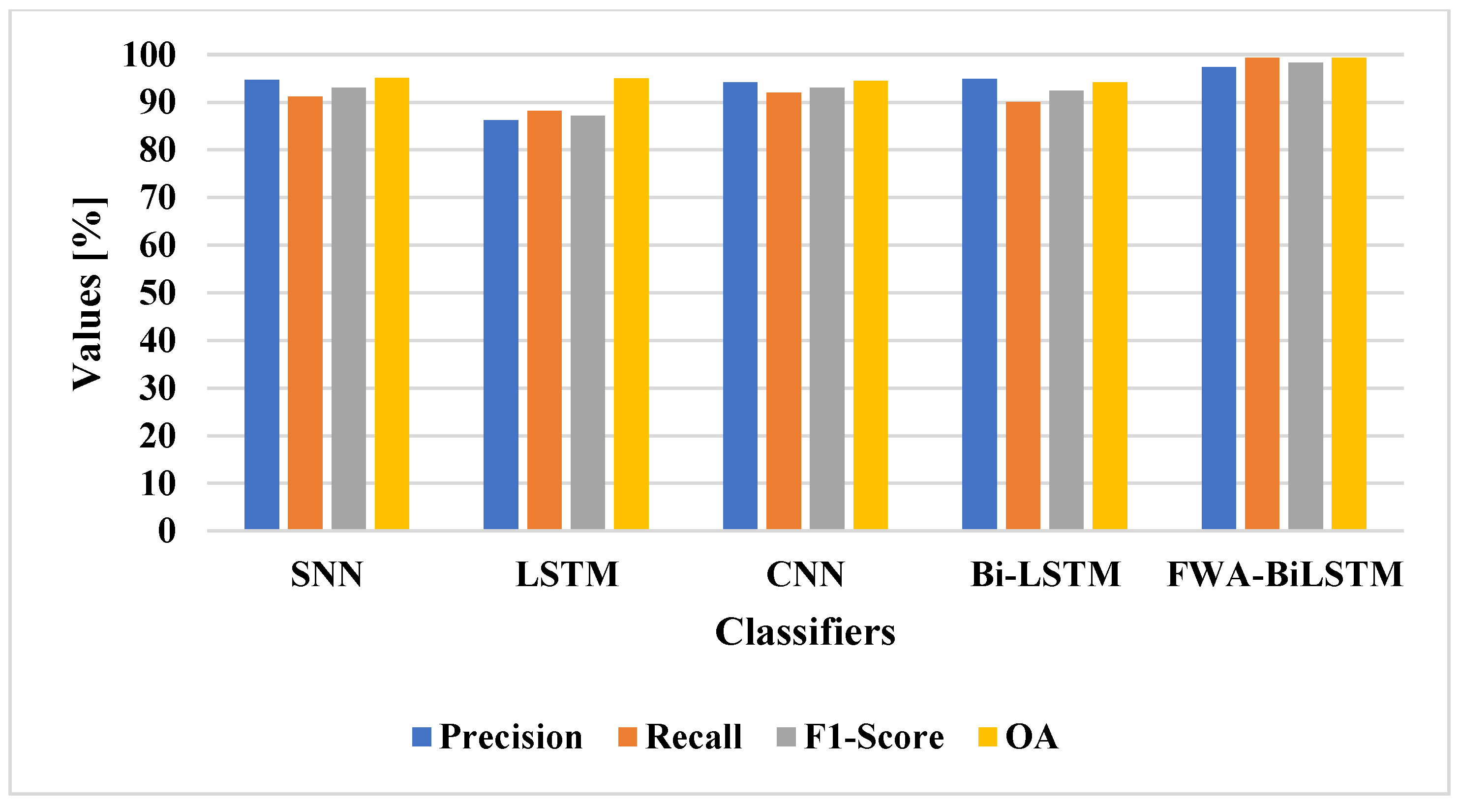
and Figure 7.

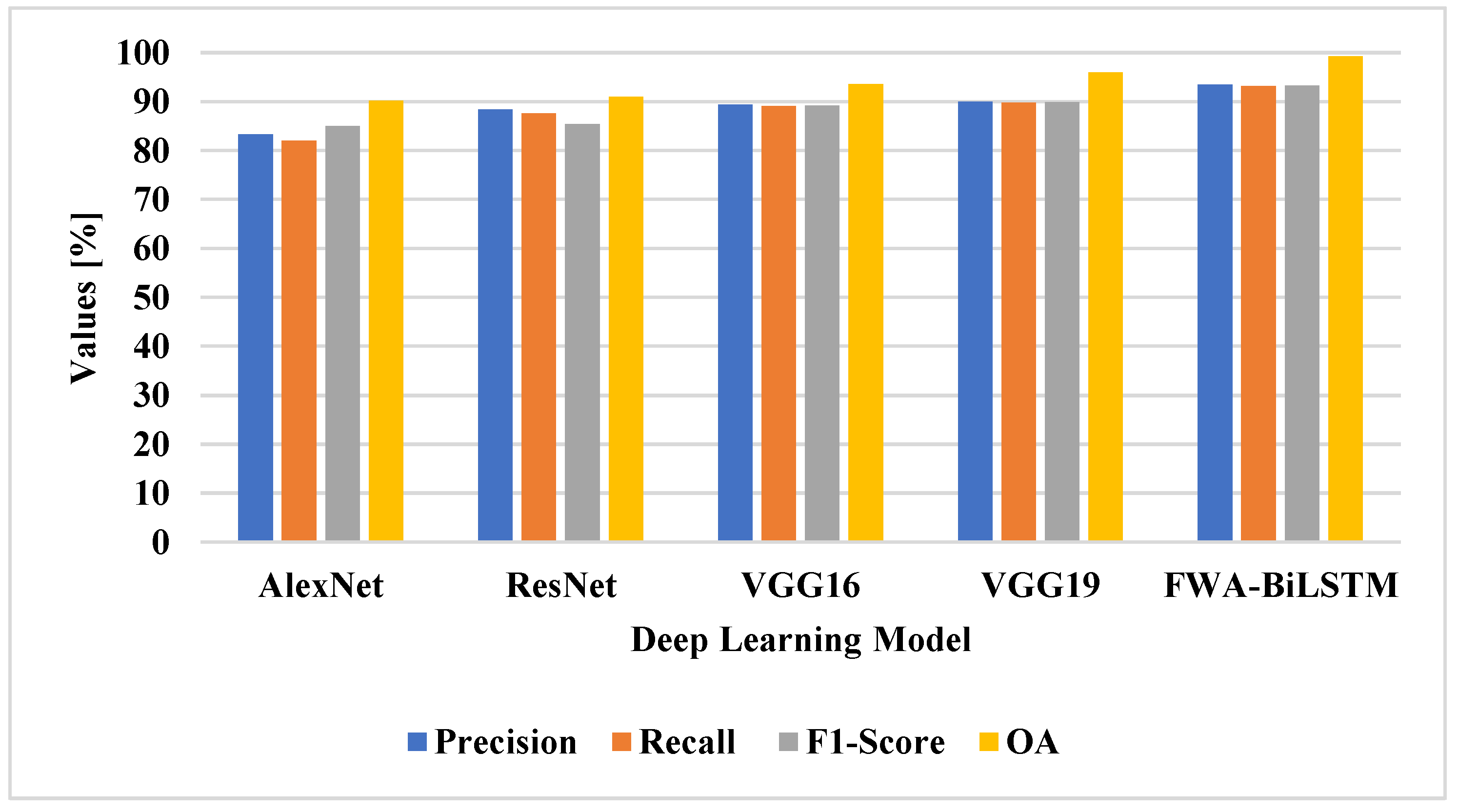
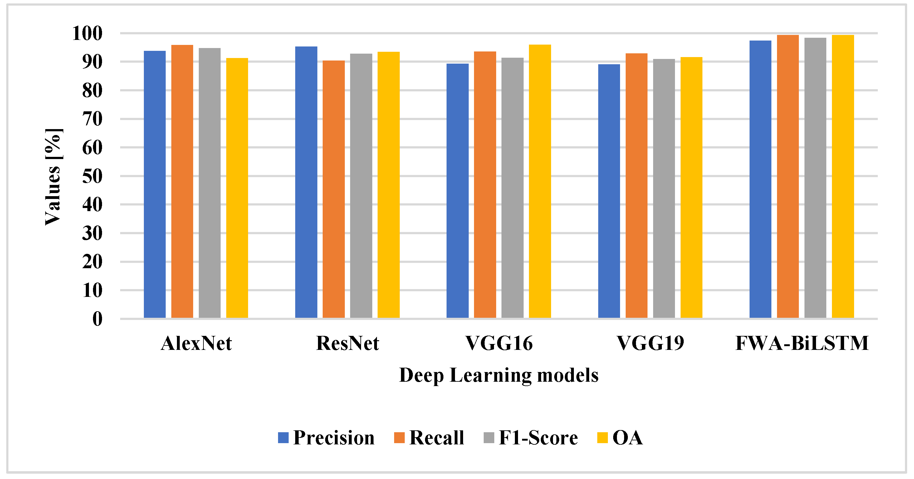
The attention layer was applied to the classifier and the performance evaluated. The attention layer increased the efficiency of the classifier for change detection, due to its efficiency in selecting the unique features for classification. The FWA-BiLSTM model used the AlexNet-VGG 16 for feature extraction, which helped to extract relevant features. The existing classifiers have lower efficiency, due to their imbalance data problem and overfitting problem in classification. The FWA-BiLSTM model obtained 93.43% precision, 93.16% recall, and 99.26% OA, whereas the CNN model had 83.34% precision, 89.31% recall, and 94.52% OA. The deep learning architectures, such as VGG19, VGG16, ResNet, and AlexNet, were applied for change detection and compared with FWA-BiLSTM, as shown in

Table 4. Performance of deep learning model on LEVIR-CD dataset.

Methods	Precision [%]	Recall [%]	F1-Score [%]	OA [%]
AlexNet	83.26	81.97	85.03	90.18
ResNet	88.34	87.58	85.36	90.96
VGG16	89.34	89.02	89.17	93.54
VGG19	89.92	89.75	89.83	95.97
FWA-BiLSTM	93.43	93.16	93.29	99.26

and Figure 8.

The FWA-BiLSTM model usedAlexNet-VGG16 for feature extraction and applied FWA to select relevant features for the BiLSTM model in classification. The existing deep learning architectures have a limitation of overfitting that degrades the performance of classification. The FWA attention technique helped to select the unique feature for classification and improved the performance of classification. The FWA-BiLSTM obtained 93.4% precision, 93.16% recall, and 99.26% OA, whereas VGG19 had 89.92% precision, 89.75% recall, and 95.97% OA.

5.2. Quantitative Analysis on SVD Dataset

To demonstrate the component of the suggested method’s contribution, ablation analysis was performed. By contrasting the model with and without the component, the system was able to determine the component’s contribution to the model. To test the effectiveness of our suggested system, modules were gradually introduced rather than deleted. The SVD dataset was a sizable remote sensing dataset, when contrasted to others. Hence, ablation analysis employed the SVD. The FWA-BiLSTM model was tested on the SVD dataset for change detection and compared with deep learning techniques. The FWA-BiLSTM model was compared with classifiers on the SVD dataset, as shown in

Table 5. Performance of classifier without attention layer on SVD dataset.

Methods	Precision [%]	Recall [%]	F1-Score [%]	OA [%]
SNN	86.84	91.28	85.46	90.08
LSTM	79.01	82.99	81.78	89.4
CNN	86.45	83.18	84.78	89.92
BiLSTM	87.03	84.76	84.96	90.87
FWA-BiLSTM	97.4	99.35	98.36	99.36

and Figure 9.

The FWA-BiLSTM model had the advantage of an attention layer to select the relevant features for the classification. The attention layer selected unique features to distinguish the changes in the images that helped to improve the efficiency of classification. CNN had an overfitting problem, while LSTM and BiLSTM model had vanishing gradient problems. The FWA-BiLSTM model obtained 97.4% precision, 99.35% recall, and 99.36% OA in change detection. The FWA-BiLSTM model with AlexNet-VGG16 feature extraction was compared with the attention layer in existing classifiers, as shown in

Table 6. Performance of classifier with attention layer on SVD dataset.

Methods	Precision [%]	Recall [%]	F1-Score [%]	OA [%]
SNN	94.95	93.18	93.01	95.12
LSTM	86.23	88.17	87.18	95.05
CNN	94.15	92.04	91.08	94.48
BiLSTM	94.88	90.06	92.4	94.19
FWA-BiLSTM	97.4	99.35	98.36	99.36

and Figure 10.

The attention layer increased the efficiency of the classifier in change detection. Nevertheless, the existing classifier suffered from the overfitting problem and imbalance data problem. The FWA-BiLSTM method selected unique features to distinguish between the changes in the images. The FWA-BiLSTM model obtained 97.4% precision, 99.35% recall, and 99.36% OA in change detection, whereas CNN with the attention layer had 94.88% precision, 90.06% recall, and 94.19% OA. The deep learning techniques were applied for the change detection on the SVD dataset and compared with FWA-BiLSTM, as shown in

Table 7. Performance of deep learning technique on SVD dataset.

Methods	Precision [%]	Recall [%]	F1-Score [%]	OA [%]
AlexNet	93.76	95.83	94.78	91.2
ResNet	95.34	90.42	92.81	93.46
VGG16	89.29	93.54	91.36	95.92
VGG19	89.05	92.9	90.93	91.57
FWA-BiLSTM	97.4	99.35	98.36	99.36

and Figure 11.

The existing deep learning techniques had the limitation of overfitting that degraded the performance of classification. The FWA-BiLSTM method selected the unique features to solve the overfitting problem that helped to distinguish the changes in the images. The FWA-BiLSTM model obtained 97.4% precision, 99.35% recall, and 99.36% OA in change detection, whereas VGG19 had 89.05% precision, 92.9% recall, and 91.57% OA.

5.3. Comparative Analysis

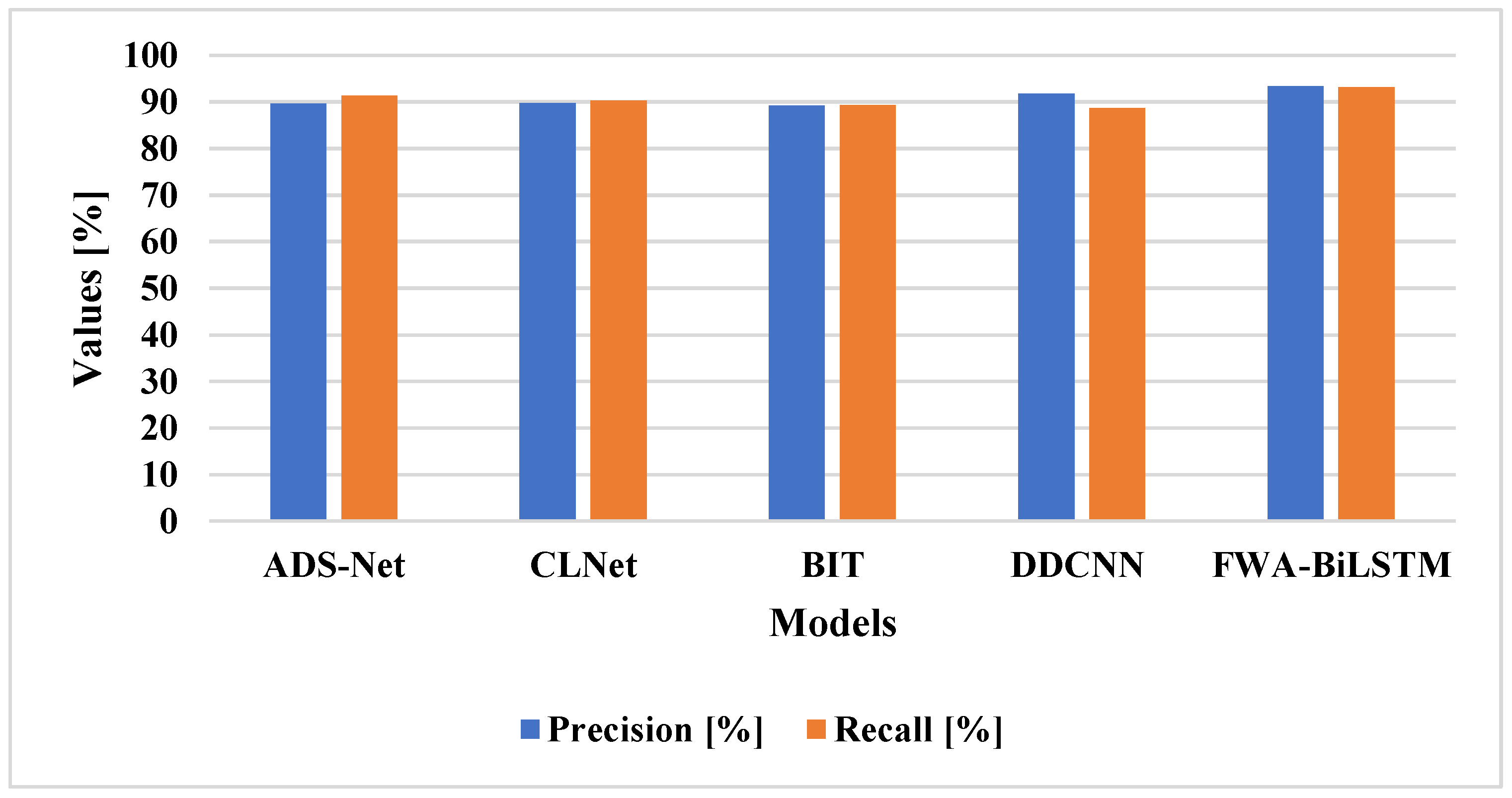
The FWA-BiLSTM was tested on two datasets, namely LEVIR-CD and SVD, and compared with other existing methods, including: ADS-Net [19], CLNet [22], BIT [23], and DDCNN [29]. The results considering the LEVIR-CD dataset are shown in

Table 8. Comparative analysis on LEVIR-CD dataset.

Methods	Precision [%]	Recall [%]	F1-Score [%]	OA [%]
ADS-Net [19]	89.67	91.36	-	-
CLNet [22]	89.8	90.3	-	98.9
BIT [23]	89.24	89.37	89.31	98.92
DDCNN [29]	91.85	88.69	90.24	98.11
FWA-BiLSTM	93.43	93.16	93.29	99.26

and Figure 12.

The existing deep learning techniques had the limitation in the form of an overfitting problem that degraded the classification performance. The FWA-BiLSTM model selected unique features to reduce the overfitting problem and increase the performance of classification. The FWA-BiLSTM model obtained 93.43% precision, 93.16% recall, and 99.26% OA, on the LEVIR-CD dataset. The FWA-BiLSTM was tested on the SVD dataset and existing deep learning techniques, including: ADS-Net [19], SNUNet-CD [20], DSAMNet [21], BIT [23], DAFCSN [26], MFCN [28], and DDCNN [29]. The results are shown in

Table 9. Comparative analysis of the SVD dataset.

Methods	Precision [%]	Recall [%]	F1-Score [%]	OA [%]
ADS-Net [19]	89.79	79.58	82.72	-
SNUNet-CD [20]	96.3	96.2	96.2	-
DSAMNet [21]	94.54	92.77	93.69	-
DAFCSN [26]	92.2	93.2	92.7	98.2
MFCN [28]	93.5	88.8	91.1	98
DDCNN [29]	96.71	92.32	94.46	98.64
BIT [23]	95.88	99.16	90.61	99.15
FWA-BiLSTM	97.4	99.35	98.36	99.36

and Figure 13.

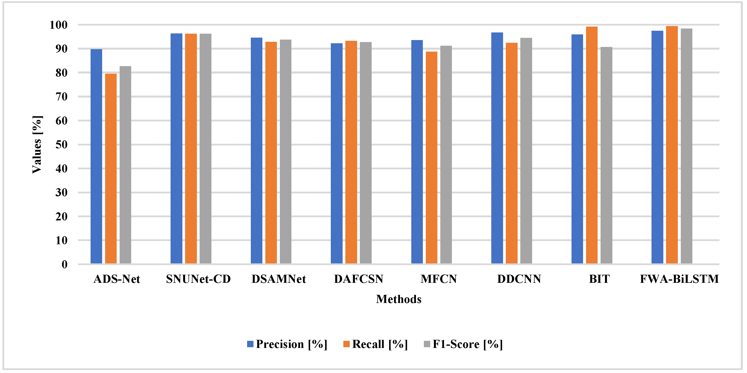
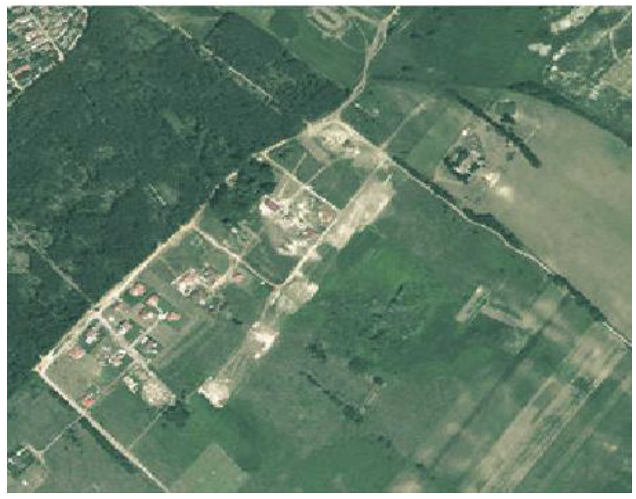
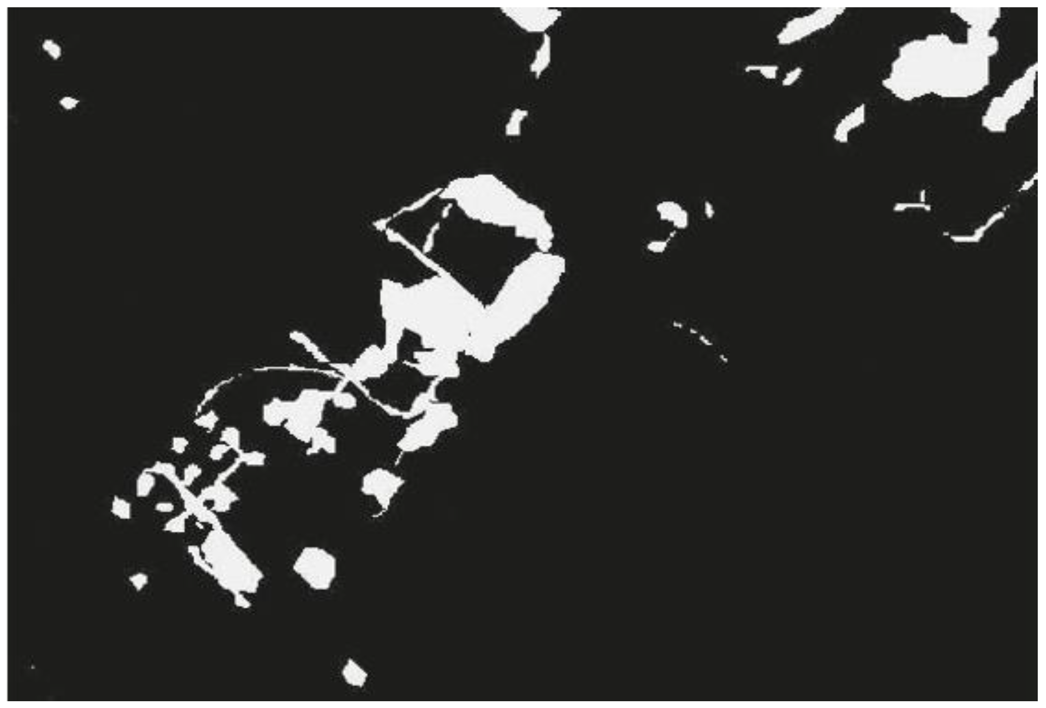
The FWA-BiLSTM model obtained higher performance than other existing techniques, due to its ability to select the unique features for classification. The FWA-BiLSTM technique provided weight values to features in order to distinguish changes in the images. The FWA-BiLSTM model obtained 97.4% precision, 99.35% recall, and 99.34% OA on the SVD dataset. Figure 14 and Figure 15 show the sample image and its visual comparison considering change detection.

5.4. Discussion

According to the obtained results, it can be seen that the proposed FWA-BiLSTM model performed better than other available methods, because it chooses the special features for classification. For the purpose of identifying changes in the images, the FWA-BiLSTM approach assigns weight values to respective features. When utilizing the SVD dataset, the FWA-BiLSTM model achieved 97.4% accuracy, 99.35% recall, and 99.34% OA. On the SVD dataset, the FWA-BiLSTM was also evaluated and compared to other deep learning methods, including: ADS-Net [19], SNUNet-CD [20], DSAMNet [21], BIT [23], DAFCSN [26], MFCN [28], and DDCNN [29]. The FWA-BiLSTM model selected special characteristics to minimize the overfitting issue and improve classification performance. In the case of the LEVIR-CD dataset, the FWA-BiLSTM model achieved 93.43% accuracy, 93.16% recall, and 99.26% OA.

6. Conclusions

Remote sensing images are very useful for change detection that may be applied in areas such as urban planning, land management, or urban management. The existing works related to CD have limitations in the form of overfitting as well as imbalanced data. This paper proposes the FWA-BiLSTM model, which enables to reduce the overfitting problem and increases the performance of classification. Normalization is applied to input images in order to reduce the pixel difference and enhance the quality of the images themselves. The AlexNet and VGG16 models are applied to extract the features from the normalized images. The extracted features are applied to FWA-BiLSTM to provide weight values to those characteristics. The FWA-BiLSTM provides higher weight to the unique features that help to distinguish the changes in the images. According to the experimental results, the suggested FWA-BiLSTM model outperformed the conventional Difference-enhancement Dense-attention Convolutional Neural Network (DDCNN) model on the basis of precision (97.4%), F1-Score (98.36), recall (99.35%), and overall accuracy (99.36%) on the SVD dataset. Future studies in this area could involve applying our technique to select relevant features and improve image classification accuracy in the case of satellite images describing changes in various urban, suburban and rural environments, such as: urban agglomerations and urban tissue, forests, crops and farmlands, river floodplains, etc.

References

- Song, L.; Xia, M.; Jin, J.; Qian, M.; Zhang, Y. SUACDNet: Attentional change detection network based on Siamese U-shaped structure. Int. J. Appl. Earth Obs. Geoinf. 2021, 105, 102597. [Google Scholar] [CrossRef]
- Liu, M.; Shi, Q.; Marinoni, A.; He, D.; Liu, X.; Zhang, L. Super-resolution-based change detection network with stacked attention module for images with different resolutions. IEEE Trans. Geosci. Remote Sens. 2021, 60, 4403718. [Google Scholar] [CrossRef]
- Zhang, H.; Lin, M.; Yang, G.; Zhang, L. ESCNET: An end-to-end superpixel-enhanced change detection network for very-high-resolution remote sensing images. IEEE Trans. Neural Netw. Learn. Syst. 2021, 1–15. [Google Scholar] [CrossRef] [PubMed]
- Hou, X.; Bai, Y.; Li, Y.; Shang, C.; Shen, Q. High-resolution triplet network with dynamic multiscale feature for change detection on satellite images. ISPRS J. Photogramm. Remote Sens. 2021, 177, 103–115. [Google Scholar] [CrossRef]
- Wang, Z.; Peng, C.; Zhang, Y.; Wang, N.; Luo, L. Fully convolutional Siamese networks based change detection for optical aerial images with focal contrastive loss. Neurocomputing 2021, 457, 155–167. [Google Scholar] [CrossRef]
- Zhang, L.; Hu, X.; Zhang, M.; Shu, Z.; Zhou, H. Object-level change detection with a dual correlation attention-guided detector. ISPRS J. Photogramm. Remote Sens. 2021, 177, 147–160. [Google Scholar] [CrossRef]
- Lei, S.; Shi, Z. Hybrid-scale self-similarity exploitation for remote sensing image super-resolution. IEEE Trans. Geosci. Remote Sens. 2022, 60, 5401410. [Google Scholar] [CrossRef]
- Zhang, Y.; Fu, L.; Li, Y.; Zhang, Y. HDFNET: Hierarchical dynamic fusion network for change detection in optical aerial images. Remote Sens. 2021, 13, 1440. [Google Scholar] [CrossRef]
- Srinivas, M.; Roy, D.; Mohan, C.K. Discriminative feature extraction from X-ray images using deep convolutional neural networks. In Proceedings of the 2016 IEEE International Conference on Acoustics, Speech and Signal Processing, Shanghai, China, 20–25 March 2016; pp. 917–921. [Google Scholar]
- Ijjina, E.P.; Mohan, C.K. Human action recognition based on recognition of linear patterns in action bank features using convolutional neural networks. In Proceedings of the 2014 13th International Conference on Machine Learning and Applications, Detroit, MI, USA, 3–6 December 2014; pp. 178–182. [Google Scholar]
- Saini, R.; Jha, N.K.; Das, B.; Mittal, S.; Mohan, C.K. ULSAM: Ultra-lightweight subspace attention module for compact convolutional neural networks. In Proceedings of the 2020 IEEE/CVF Winter Conference on Applications of Computer Vision, Snowmass Village, CO, USA, 1–5 March 2020; pp. 1616–1625. [Google Scholar] [CrossRef]
- Deepak, K.; Chandrakala, S.; Mohan, C.K. Residual spatiotemporal autoencoder for unsupervised video anomaly detection. Signal Image Video Process. 2021, 15, 215–222. [Google Scholar] [CrossRef]
- Roy, D.; Murty, K.S.R.; Mohan, C.K. Unsupervised universal attribute modeling for action recognition. IEEE Trans. Multimed. 2018, 21, 1672–1680. [Google Scholar] [CrossRef]
- Perveen, N.; Roy, D.; Mohan, C.K. Spontaneous expression recognition using universal attribute model. IEEE Trans. Image Process. 2018, 27, 5575–5584. [Google Scholar] [CrossRef] [PubMed]
- Roy, D.; Ishizaka, T.; Mohan, C.K.; Fukuda, A. Vehicle trajectory prediction at intersections using interaction based generative adversarial networks. In Proceedings of the 2019 IEEE Intelligent Transportation Systems Conference, Auckland, New Zealand, 27–30 October 2019; pp. 2318–2323. [Google Scholar]
- Roy, D.; Mohan, C.K. Snatch theft detection in unconstrained surveillance videos using action attribute modelling. Pattern Recognit. Lett. 2018, 108, 56–61. [Google Scholar] [CrossRef]
- Kiran, P.; Parameshachari, B.D.; Yashwanth, J.; Bharath, K.N. Offline signature recognition using image processing techniques and back propagation neuron network system. SN Comput. Sci. 2021, 2, 196. [Google Scholar] [CrossRef]
- Li, X.; Du, Z.; Huang, Y.; Tan, Z. A deep translation (GAN) based change detection network for optical and SAR remote sensing images. ISPRS J. Photogramm. Remote Sens. 2021, 179, 14–34. [Google Scholar] [CrossRef]
- Wang, D.; Chen, X.; Jiang, M.; Du, S.; Xu, B.; Wang, J. ADS-Net: An attention-based deeply supervised network for remote sensing image change detection. Int. J. Appl. Earth Obs. Geoinf. 2021, 101, 102348. [Google Scholar]
- Fang, S.; Li, K.; Shao, J.; Li, Z. SNUNet-CD: A densely connected Siamese network for change detection of VHR images. IEEE Geosci. Remote Sens. Lett. 2021, 19, 8007805. [Google Scholar] [CrossRef]
- Shi, Q.; Liu, M.; Li, S.; Liu, X.; Wang, F.; Zhang, L. A deeply supervised attention metric-based network and an open aerial image dataset for remote sensing change detection. IEEE Trans. Geosci. Remote Sens. 2022, 60, 5604816. [Google Scholar] [CrossRef]
- Zheng, Z.; Wan, Y.; Zhang, Y.; Xiang, S.; Peng, D.; Zhang, B. CLNet: Cross-layer convolutional neural network for change detection in optical remote sensing imagery. ISPRS J. Photogramm. Remote Sens. 2021, 175, 247–267. [Google Scholar] [CrossRef]
- Chen, H.; Qi, Z.; Shi, Z. Remote sensing image change detection with transformers. IEEE Trans. Geosci. Remote Sens. 2021, 60, 5607514. [Google Scholar] [CrossRef]
- Peng, D.; Zhang, Y.; Guan, H. End-to-end change detection for high resolution satellite images using improved UNet++. Remote Sens. 2019, 11, 1382. [Google Scholar] [CrossRef]
- Zhang, C.; Yue, P.; Tapete, D.; Jiang, L.; Shangguan, B.; Huang, L.; Liu, G. A deeply supervised image fusion network for change detection in high resolution bi-temporal remote sensing images. ISPRS J. Photogramm. Remote Sens. 2020, 166, 183–200. [Google Scholar] [CrossRef]
- Chen, J.; Yuan, Z.; Peng, J.; Chen, L.; Huang, H.; Zhu, J.; Li, Y.; Li, H. DASNet: Dual attentive fully convolutional Siamese networks for change detection in high-resolution satellite images. IEEE J. Sel. Top. Appl. Earth Obs. Remote Sens. 2020, 14, 1194–1206. [Google Scholar] [CrossRef]
- Jiang, H.; Hu, X.; Li, K.; Zhang, J.; Gong, J.; Zhang, M. PGA-SiamNet: Pyramid feature-based attention-guided Siamese network for remote sensing orthoimagery building change detection. Remote Sens. 2020, 12, 484. [Google Scholar] [CrossRef] [Green Version]
- Li, X.; He, M.; Li, H.; Shen, H. A combined loss-based multiscale fully convolutional network for high-resolution remote sensing image change detection. IEEE Trans. Geosci. Remote Sens. 2022, 19, 8017505. [Google Scholar] [CrossRef]
- Peng, X.; Zhong, R.; Li, Z.; Li, Q. Optical remote sensing image change detection based on attention mechanism and image difference. IEEE Trans. Geosci. Remote Sens. 2020, 59, 7296–7307. [Google Scholar] [CrossRef]
- Song, K.; Cui, F.; Jiang, J. An Efficient Lightweight Neural Network for Remote Sensing Image Change Detection. Remote Sens. 2021, 13, 5152. [Google Scholar] [CrossRef]
- Chen, J.; Wan, Z.; Zhang, J.; Li, W.; Chen, Y.; Li, Y.; Duan, Y. Medical image segmentation and reconstruction of prostate tumor based on 3D AlexNet. Comput. Meth. Prog. Biomed. 2021, 200, 105878. [Google Scholar] [CrossRef] [PubMed]
- Lu, S.; Wang, S.H.; Zhang, Y.D. Detection of abnormal brain in MRI via improved AlexNet and ELM optimized by chaotic bat algorithm. Neural Comput. Appl. 2021, 33, 10799–10811. [Google Scholar] [CrossRef]
- Chen, H.C.; Widodo, A.M.; Wisnujati, A.; Rahaman, M.; Lin, J.C.W.; Chen, L.; Weng, C.E. AlexNet convolutional neural network for disease detection and classification of tomato leaf. Electronics 2022, 11, 951. [Google Scholar] [CrossRef]
- Xu, P.; Zhao, J.; Zhang, J. Identification of intrinsically disordered protein regions based on deep neural network-VGG16. Algorithms 2021, 14, 107. [Google Scholar] [CrossRef]
- Montaha, S.; Azam, S.; Rafid, A.K.M.R.H.; Ghosh, P.; Hasan, M.Z.; Jonkman, M.; De Boer, F. BreastNet18: A high accuracy fine-tuned VGG16 model evaluated using ablation study for diagnosing breast cancer from enhanced mammography images. Biology 2021, 10, 1347. [Google Scholar] [CrossRef] [PubMed]
- Afaq, Y.; Manocha, A. Analysis on change detection techniques for remote sensing applications: A review. Ecol. Inform. 2021, 63, 101310. [Google Scholar] [CrossRef]
- Singla, P.; Duhan, M.; Saroha, S. An ensemble method to forecast 24-h ahead solar irradiance using wavelet decomposition and BiLSTM deep learning network. Earth Sci. Inform. 2022, 15, 291–306. [Google Scholar] [CrossRef] [PubMed]
- Lu, W.; Li, J.; Wang, J.; Qin, L. A CNN-BiLSTM-AM method for stock price prediction. Neural Comput. Appl. 2021, 33, 4741–4753. [Google Scholar] [CrossRef]
- Chen, H.; Shi, Z. A spatial-temporal attention-based method and a new dataset for remote sensing image change detection. Remote Sens. 2020, 12, 1662. [Google Scholar] [CrossRef]
- Lebedev, M.A.; Vizilter, Y.V.; Vygolov, O.V.; Knyaz, V.A.; Rubis, A.Y. Change detection in remote sensing images using conditional adversarial networks. Int. Arch. Photogramm. Remote Sens. Spat. Inf. Sci. 2018, 42, 565–571. [Google Scholar] [CrossRef] [Green Version]
- Yang, L.; Chen, Y.; Song, S.; Li, F.; Huang, G. Deep Siamese networks-based change detection with remote sensing images. Remote Sens. 2021, 13, 3394. [Google Scholar] [CrossRef]
Figure 1.
The FWA-BiLSTM model in change detection.
Figure 2.
CNN model for feature extraction process.
Figure 3.
AlexNet architecture for feature extraction.
Figure 4.
VGG16 architecture in feature extraction.
Figure 5.
Attention unit with BiLSTM model for classification.
Figure 6.
Classifier comparison of FWA-BiLSTM model on LEVIR-CD dataset.
Figure 7.
Classifier with attention layer on LEVIR-CD dataset.
Figure 8.
Performance of deep learning on LEVIR-CD dataset.
Figure 9.
Classifier compared with FWA-BiLSTM model on SVD dataset.
Figure 10.
Classifier with attention layer on SVD dataset.
Figure 11.
Deep learning techniques on SVD dataset.
Figure 12.
Comparative analysis of the LEVIR-CD dataset.
Figure 13.
Comparative analysis of the SVD dataset.
Figure 14.
Reference sample image.
Figure 15.
Visual comparison on change detection.