
MFATNet: Multi-Scale Feature Aggregation via Transformer for Remote Sensing Image Change Detection


1
Computer Network Information Center, Chinese Academy of Sciences, Beijing 100190, China
2
University of the Chinese Academy of Sciences, Beijing 100049, China
*
Author to whom correspondence should be addressed.
Remote Sens. 2022, 14(21), 5379; https://doi.org/10.3390/rs14215379
Submission received: 20 September 2022
/
Revised: 22 October 2022
/
Accepted: 25 October 2022
/
Published: 27 October 2022
(This article belongs to the Section Remote Sensing Image Processing)
Abstract
:In recent years, with the extensive application of deep learning in images, the task of remote sensing image change detection has witnessed a significant improvement. Several excellent methods based on Convolutional Neural Networks and emerging transformer-based methods have achieved impressive accuracy. However, Convolutional Neural Network-based approaches have difficulties in capturing long-range dependencies because of their natural limitations in effective receptive field acquisition unless deeper networks are employed, introducing other drawbacks such as an increased number of parameters and loss of shallow information. The transformer-based methods can effectively learn the relationship between different regions, but the computation is inefficient. Thus, in this paper, a multi-scale feature aggregation via transformer (MFATNet) is proposed for remote sensing image change detection. To obtain a more accurate change map after learning the intra-relationships of feature maps at different scales through the transformer, MFATNet aggregates the multi-scale features. Moreover, the Spatial Semantic Tokenizer (SST) is introduced to obtain refined semantic tokens before feeding into the transformer structure to make it focused on learning more crucial pixel relationships. To fuse low-level features (more fine-grained localization information) and high-level features (more accurate semantic information), and to alleviate the localization and semantic gap between high and low features, the Intra- and Inter-class Channel Attention Module (IICAM) are integrated to further determine more convincing change maps. Extensive experiments are conducted on LEVIR-CD, WHU-CD, and DSIFN-CD datasets. Intersection over union (IoU) of 82.42 and F1 score of 90.36, intersection over union (IoU) of 79.08 and F1 score of 88.31, intersection over union (IoU) of 77.98 and F1 score of 87.62, respectively, are achieved. The experimental results achieved promising performance compared to certain previous state-of-the-art change detection methods.
1. Introduction
Change detection in remote sensing images aims to determine the changes in the region of interest of a bi-temporal image, which is essentially the task of accurate classification of pixels in the image. The pixels in the same region but acquired at different times are usually classified as changed or unchanged by comparing the co-registered images [1]. These changes in areas of interest (i.e., forests, buildings, roads, etc.) have crucial applications in disaster monitoring, urban planning, and military surveillance [2,3]. Therefore, the development of effective and efficient change detection methods is essential. However, traditional change detection algorithms need complex manual feature design, such as spectral-based features and texture-based features, which have insufficient generalization performance as well as labor-intensive costs [2,4,5,6]. Recently, with the increasing abundance of earth observation devices, the resolution and data accessibility of remote sensing images have been increasing, introducing new opportunities for remote sensing image change detection methods. Accompanied by the steady expansion of deep learning methods, visual representations from a large amount of data can be increasingly and effectively utilized. Automatic change detection methods can also streamline the detection procedures and considerably minimize human time consumption [6,7,8].
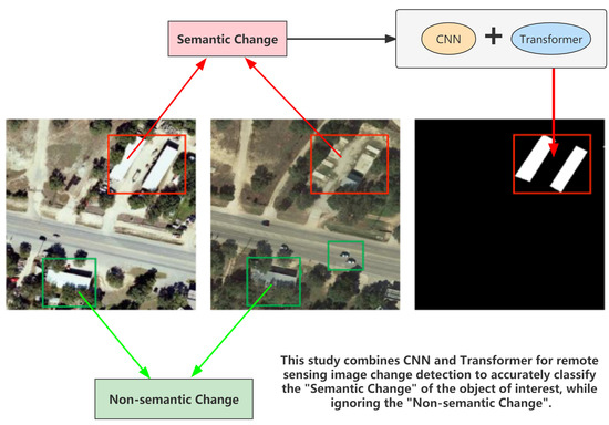
Unlike the segmentation task that also precisely classifies the pixels, the change detection data are more complicated in the presence of many factors that introduce “non-semantic changes” caused by co-registered images [9]. “Non-semantic changes” are variations in brightness and shadows on the same object caused by different seasons (whether there is snow on the identical object in summer and winter) or different lighting conditions for the same area. It can be concluded that the change map given by a decent change detection method must possess two characteristics: (1) the capability to determine high-level semantic information of the intended object; this ought not contain non-semantic changes; (2) the capability to focus on the changes of the object of interest in the intricate scenes of the remote sensing images [2,7,10,11].
Convolutional Neural Networks (CNNs) have surfaced prolifically in recent years, and methods and components of neural networks have been used in several segmentation tasks to extract meaningful visual representations in change detection [2,3,4,5,7,12,13,14]. Fully Convolution Network (FCN) [15] was a pioneer in segmentation tasks and has inspired many change detection models [5]. Subsequently, Unet [16] emerged as the benchmark model for many change detection tasks, and several successors have benefited from its philosophy [5,9,17]. Furthermore, several efforts have been undertaken on the enhancement of the depth features extracted by the backbone. In paper [4], Feature Pyramid Network (FPN) was used to integrate the top-down multi-scale information. Papers [9,17] fuse the multi-scale change maps to derive improved result maps. Moreover, there are features such as [14,18] that utilize spatial or channel attention to select features that are more effective for the results. Despite the impressive development of change detection with the support of Convolutional Neural Networks, there are still certain inherent limitations to the CNN-based approaches. The size of the convolutional kernel naturally restricts the size of the perceptual field and obtains a larger effective receptive field that requires deeper and deeper networks or stacked convolution [12,19,20], dilated convolution [19], etc., which in turn introduces the disadvantage of loss of subtle and local semantic information and increased computing time. However, the rise of transformer structure in the field of computer vision [21,22,23] seems to bring more complexity to the above problems.
Transformer structures have previously been broadly adopted in the field of Natural Language Processing (NLP) for learning long-range dependencies among the diverse words or phrases in sequences to sequences tasks, and for which such a global concept can be considered to address the above-mentioned difficulties. ViT [21] pioneered the application of transformer to vision missions by sub-patching images, and subsequently evolved hierarchies like PVT [23] and SwinTransformer [22]. While the BiT [2] piloted to combine CNN and transformer for the change detection task in the field of remote sensing image change detection, MSTCDNet [7] utilizes the SwinTransformer [22] block to process the multi-scale features extracted by the CNN backbone network, respectively. The changeformer [3] leverages pure transformer hierarchical structure. These transformer-based methods can capture a larger effective perceptual field compared to CNN.
When we use the transformer architecture in an image, a critical step is the tokenizer for subsequent processing. However, with regard to previous work—such as [7], plainly slicing images into non-overlapping patches to construct tokens; [2], constructing compact semantic tokens via point-to-point convolution and Softmax; and [24], further exploiting plain tokens by changing the transformer structure—none of them further constructs tokens at the token level. We intuitively introduce the Spatial Attention Module to obtain the spatial attention feature map and then perform Softmax operations to give the compact semantic tokens stronger spatial location information, which we call Spatial Semantic Tokenizer (SST).
Moreover, we utilize a multi-scale to fuse high-level semantic and low-level localization information. Then the overlap effect is brought about due to upsampling when different scale features are fused. In paper [25], the effect is eliminated by performing one convolution on the fused feature map at a time. Paper [9] introduces the channel attention module (CAM) to select more discriminative features. We likewise introduce CAM in the hope that not only the selection in the channel dimension but also the representations from within the features at different scales are utilized.
Inspired by the above method, a Multi-scale Feature Aggregation via Transformer Network (MFATNet) has been proposed to model the rich contextual relationships in the bi-temporal remote sensing images and the fusion of individual scale features to exploit the representations at different levels. The proposed empirical conception stems from the fusion of multi-scale features in the CNN-based approach that allows simultaneously taking into account both low-level representations with more accurate localization information and high-level representations with stronger semantic information about the object. Meanwhile, we follow the semantic tokenizer in BiT [2] and introduce the Spatial Attention Module, resulting in the design of a Spatial Semantic Tokenizer (SST) for a more effective transformer to capture spatial context, which can highlight the learning of the region of interest more compared to the simple flatten. While performing the multi-scale feature fusion, given the existence of localization and the semantic gap between pixels of different features, Intra- and Inter-class Channel Attention Module (IICAM) is introduced to smoothen the gap between different features while accounting for higher discrimination between the feature groups.
The backbone of the proposed MFATNet is the Siamese ResNet18 [26], which uses the last four of the five stages to primitively extract the features of the bi-temporal images . The tokens obtained from different scales are combined into a single token and sent to the transformer to capture the long-range dependencies. The resulting context-rich tokens are further split and converted into the raw feature map shape, where the four feature maps are concatenated and the final result map is generated after IICAM.
As a result of our work, the following contributions have been made.
- We propose a novel MFATNet that utilizes the transformer structure to learn the feature intra-relationships at different scales extracted by the ResNet and then aggregate these features to obtain stronger semantic and localization representations.
- SST is proposed to obtain tokens with strengthened semantic representations which enable the transformer to learn the relationships between critical regions.
- To alleviate semantic gaps and localization errors between multi-scale feature aggregation, IICAM is integrated.
- Extensive experiments have been conducted on the LEVIR-CD, WHU-CD, and DSIFN-CD datasets, and the F1 scores and IoU have achieved promising performance.
2. Related Work
2.1. Change Detection Method Based on Convolutional Neural Network
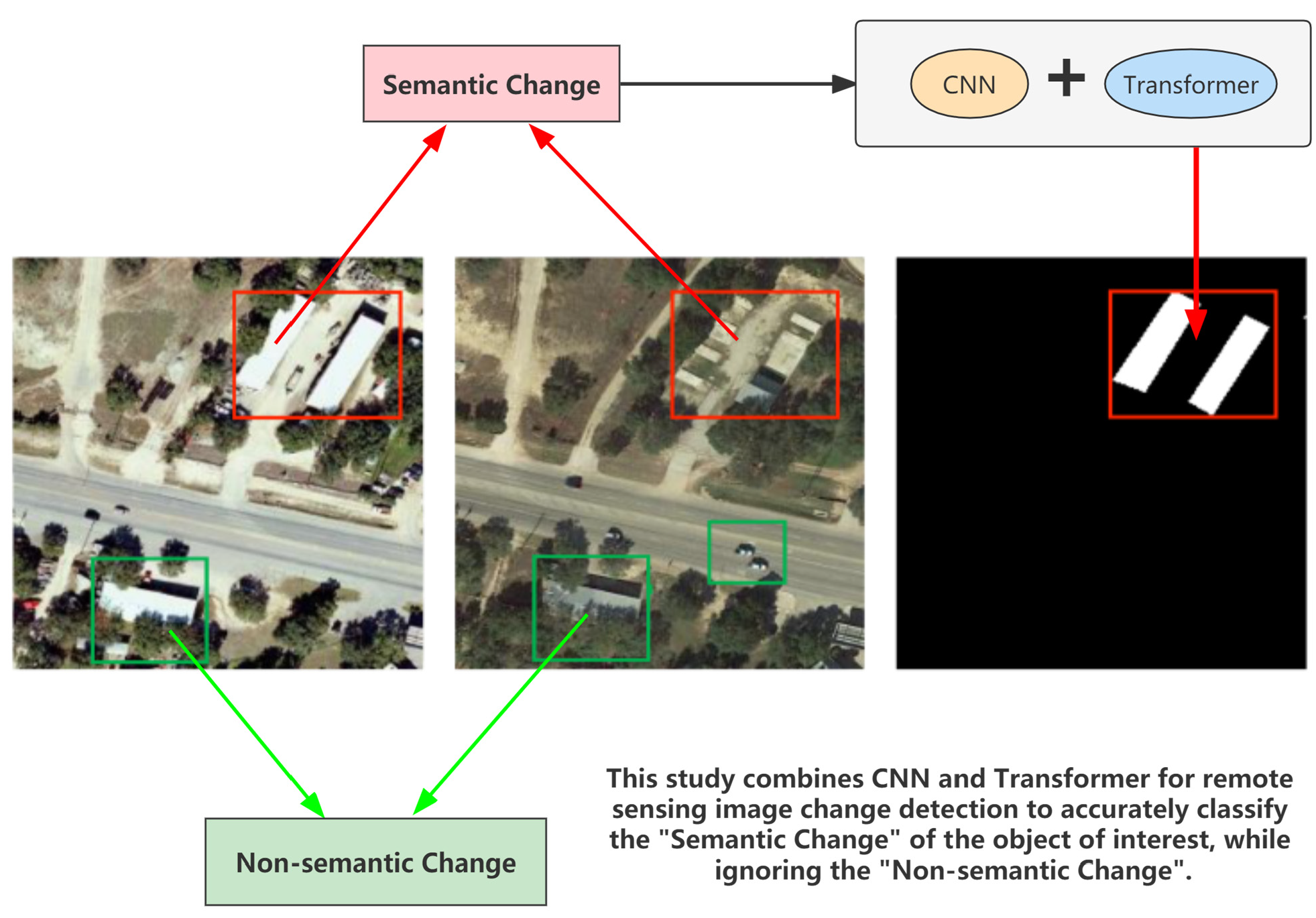
Methods of change detection which have excellent performance in recent years have been based on deep learning because of their ability to extract powerful discriminative features. In an earlier period, the prevailing practice [27,28,29] was to obtain the semantic results of the bi-temporal images separately and then compare them to produce the change maps. Subsequently, some work [8,30] was conducted by predicting co-registered images partitioned by patches to directly obtain the change maps. With the development of semantic segmentation [15,16,31,32], new inspiration for remote sensing image change detection brought due to change detection is also a task of accurate segmentation of pixels; thus, semantic segmentation methods have given a significant promotion to deep learning-based change detection methods. In these papers [4,5,9,10,12,13,14,17,33,34,35,36,37,38,39,40], the encoder–decoder architecture is used to classify the pixels and generate a change result map, often with a trade-off between efficiency and effectiveness. When information fusion is performed, the existing change detection methods can be classified as image-level and feature-level, as demonstrated in Figure 1. In the image-level fusion [5,17,33,40,41] method, the bi-temporal images are concatenated along the channel dimension before feeding them to the neural network. The feature-level fusion [4,10,12,14,18,19,34,36,37,38,39,42] method fuses the bi-temporal images with features extracted by the neural network. The above-mentioned CD methods suffer from the natural disadvantages of the CNN local receptive field and have some difficulties in perceiving the relationship between the changed region and other regions. However, this problem is alleviated in this paper by utilizing the transformer.
2.2. Transformer-Based Change Detection Methods
The recent remarkable success of transformers in Natural Language Processing has driven its application to the vision tasks. Vision Transformer (ViT) [21] is the pioneering work on the application of the transformer to vision tasks by dividing the images into non-overlapping patches, and also has some driving works [22,43]. The transformer has also made substantial progress in the semantic segmentation task [44,45,46], which also classifies the pixel points precisely. There are certain works to apply the transformer to remote sensing image change detection, but BiT [2] reveals the significant potential of the transformer in remote sensing image change detection. Subsequently, MSTCDNet [7] and ChangeFormer [3] further develop the application of the transformer to the change detection tasks. The former addressed the multi-scale features with the help of SwinTransformer block, while the latter adopted a pure transformer structure. Intuitively, the change in the area of interest is usually large, and the Convolutional Neural Networks obtain a larger receptive field by means of dilated convolution, deepening networks, etc. However, there is a loss of some subtle information. The transformer is inherently able to compute the global receptive field of the input, providing stronger context modeling capabilities across pixels, which is beneficial for high-resolution remote sensing images where the scene is more complicated and where objects may be distributed over arbitrary pixels on the image (e.g., buildings, agricultural land).
3. Materials and Methods
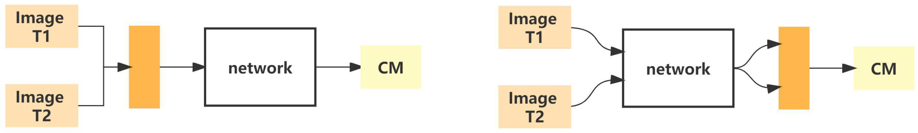
In this section, the proposed approach is described in detail, as shown in Figure 2. When there is a pair of bi-temporal images, the features are first extracted by ResNet18, and here only the feature maps of the last four stages of ResNet are used. A Spatial Attention Tokenizer (SST) is applied to each of the extracted feature maps at different scales for each stage separately to convert them into tokens. These tokens are further merged and fed into the transformer structure to learn the relationship between the pixel in different regions. Until here, the feature maps with stronger representation capabilities are obtained, as compared to those extracted with pure CNN methods. The absolute difference is used as the feature fusion method, and the feature map is recovered to the raw size and passed through a classifier to produce the final change map.
3.1. Multi-Scale Feature Extraction
In recent years, several impressive backbone networks have emerged, such as ResNet. In the proposed work, ResNet18 is used as a feature extractor, considering that the transformer can extract global information and a deeper Convolutional Neural Network is not necessary to acquire a larger respective field. Given that the input is a bi-temporal image, the parameter-sharing Siamese ResNet18 is used to determine the features of the two images separately. When a image is fed into ResNet18, the feature maps extracted from the last four of the five stages of ResNet form the multi-scale feature maps that are subsequently used by the transformer. Compared to the original image size, the feature map size is reduced by times for each stage from light to dark, respectively.
3.2. Spatial Semantic Tokenizer
The transformer is unable to accept images directly as matrices but as vectors. ViT [21] is an excellent application of images on the transformer architecture, which divides images into non-overlapping patches for image classification and achieves better performance compared to Convolutional Neural Networks. However, ViT requires large-scale training datasets to perform well and has a heavy computational burden. Another work from the same period as ViT, visual transformer [43], applied the transformer after constructing semantic tokens by extracting the features from images using Convolutional Neural Networks, which has the merit of avoiding a large computational burden and achieving commendable performance at the same time. Considering that remote sensing images are usually of high resolution, the scheme provided by the latter is adopted in this work.
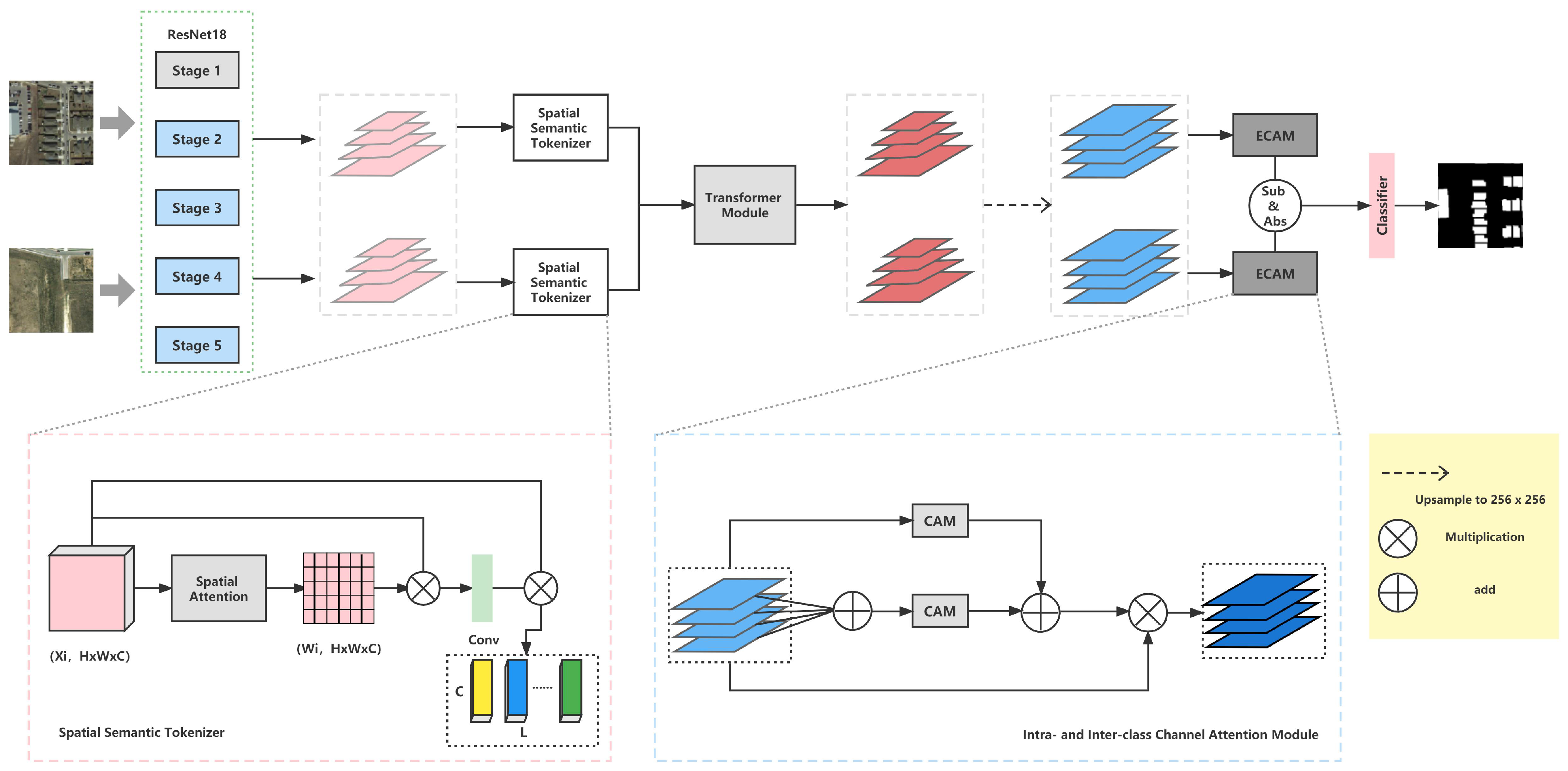
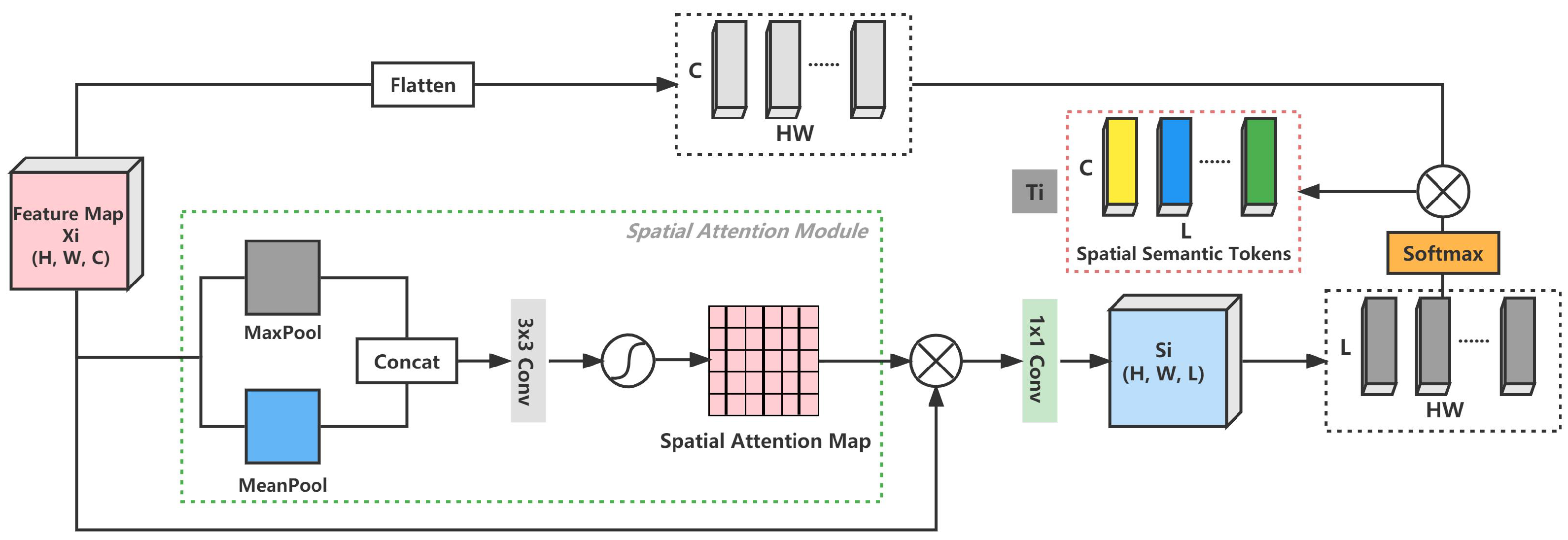
Therefore, our thought is to process the image as a vector in the change detection task. With the help of dimensional correlation functions in a deep learning open source framework, the conversion of to , where are the height, width, and channel of the input image respectively, can be easily implemented. Actually, each pixel in the vector is a token similar to a word in a sentence. However, the direct flattening does not consider the redundant information in the image. Therefore, to make the subsequent transformer more effective in learning long-range dependencies, a spatial location enhancement for such a dimensional transformation called Spatial Semantic Tokenizer (SST) is imposed, as demonstrated in Figure 3. Each token in the final semantic tokens represents a semantic concept in the image.
More specifically, each scale feature extracted by the Convolutional Neural Network is indicated by , where correspond to the height and width of each scale feature map, respectively, and C is the number of channels, and corresponds to the last four stages of ResNet. SST is divided into two branches: One branch is the plain flattening of the feature map for each channel into a vector form, and the dimension of changes from to . The other branch is to utilize the spatial attention map obtained from the Spatial Attention Module to compute the weighted average sum of each pixel of , and then perform a point-wise convolution to compute the spatial semantic map where L denotes the number of semantic tokens. Similarly, the dimension of changes from to , and the Softmax operation along the dimension is applied. Eventually, the tokens obtained from the two branches are multiplied to obtain the final spatial semantic tokens . The formulation of the Spatial Semantic Tokenizer is mentioned below.
where indicates the Spatial Attention Module, which performs maximum pooling and mean pooling on the feature map after stacking, and then the sigmoid activation function is employed. represents the point-wise convolution with learnable parameters . is Softmax operation.
3.3. Multi-Scale Transformer
In the field of Natural Language Processing, transformer architecture has been extensively used and has brought significant progress. In the field of change detection, excellent transformer-based models such as BiT [2], a model, and ChangeFormer [3], a pure transformer model, have emerged, both achieving impressive performance on the LEVIR-CD and DSIFN-CD datasets. However, neither of them considers the multi-scale feature information available using Convolutional Neural Networks. However, MSTDSNet-CD [7] leverages the hierarchical property of SwinTransformer to utilize the multi-scale feature maps extracted by ResNet. Compared to MSTDSNet-CD, instead of employing multiple SwinTransformer Blocks, there is just one transformer encoder and decoder. This is explained in detail in the following part.
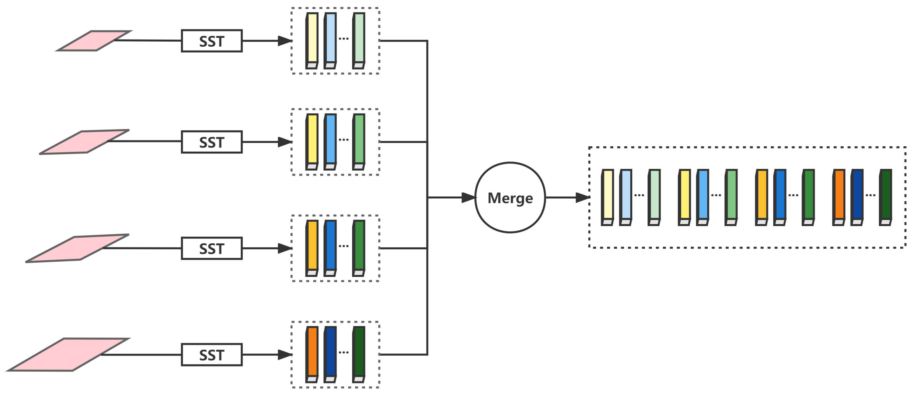
When the multi-scale feature maps are obtained, the SST module is used to yield the semantic tokens. Further, the merge operation forms a larger token out of multiple semantic tokens. Specifically, each set of semantic tokens is concatenated along the L-dimension. The diagram of the merging of the token group is represented in Figure 4. The formula for merging multiple token groups is expressed as follows.
where denotes T, the semantic tokens corresponding to each scale feature map. represents the concatenate operation. represents the tokens after the merger.
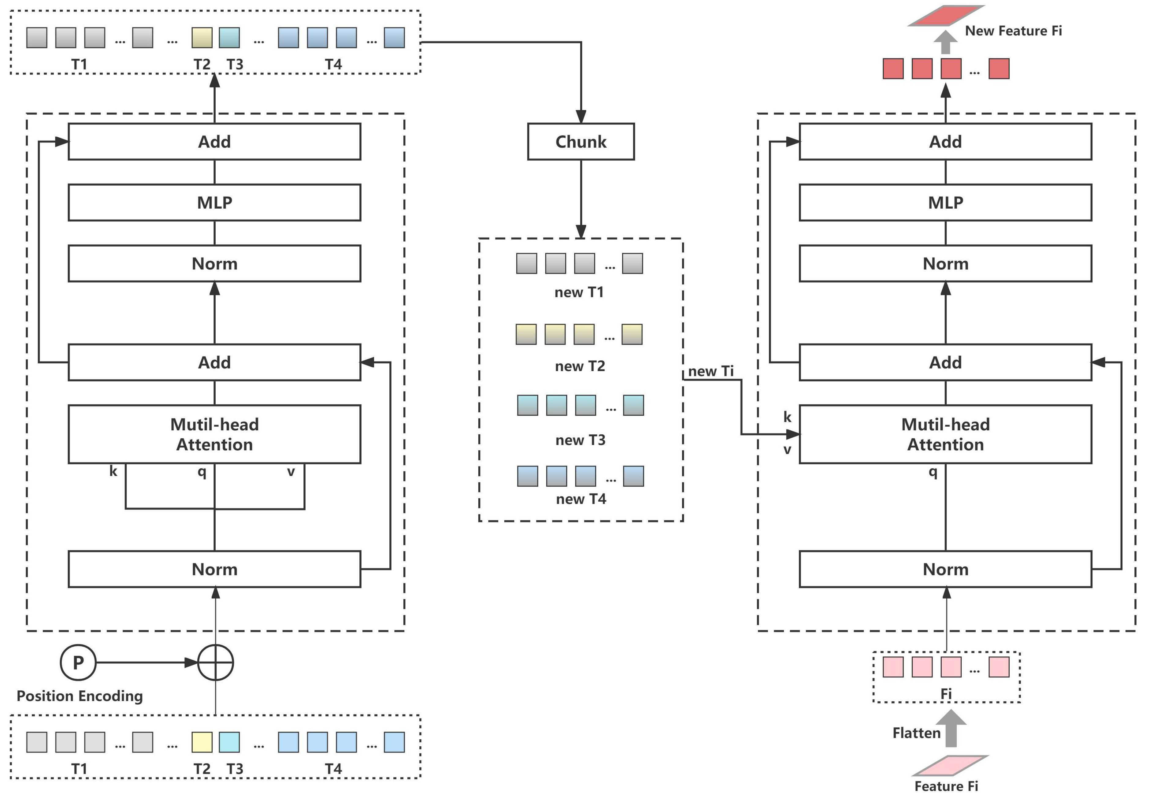
A token representation containing rich space–time context is obtained through the tokenizer operation. It is expected to capture the global semantic relations of this representation; thus, the transformer is utilized owing to its property of capturing long-range dependencies. To learn the representation of the region of interest with respect to other regions of relevance, groups of semantic tokens are fed into the transformer. The transformer employed in this paper is divided into two parts, encoder and decoder, as depicted in Figure 5. Given the special treatment of tokens, the structure of the transformer need not be changed too much to accommodate the learning of multi-scale features. The transformer consists of Multi-headed Self-Attention (MSA) and Multi-layer Perceptron (MLP), using pre-norm for better stability. The merged semantic tokens are fed into the encoder of the transformer, and the initially learned representations of the relevance of different regions are obtained, and then the new tokens obtained to get the same number of tokens are chunked as the multi-scale features and are eventually fed into the decoder for further learning.
When the tokens are fed into the transformer to compute self-attention, Q, K, and V are computed by token T, where Q, K, and denote Query, Key, and Value, respectively. It must be noted that token T is fed into the transformer before performing the learnable position encoding (abbreviated as ), which is taken from the experience in BiT [2]. can guide the modeling of the transformer in a long-range context owing to the encoding of the relative or absolute position information of elements in the token. At each layer l, Q, K, and V are computed as follows:
where are learnable parameters, and d is the number of channel dimensions of the . The formula for computing the self-attention head is as follows:
where means the Softmax operation along the channel dimension. However, the core construction of the mentioned transformer is the MSA, which computes multiple independent attention heads in parallel and then concatenates their values, with each head differing in the inconsistency of the learnable linear change matrices for computing Q, K, and V. The formulation of MSA is expressed as follows:
where represents the concatenate operation, , is the linear projection matrices, and h denotes the number of heads. Yet the computation of the MSA in the decoder and encoder of the transformer is different, as can be seen from Figure 5, where Q comes from the semantic token and feature map , respectively. The other primary component of the transformer, the MLP, comprises two linear projection layers, where one of the projection changes performs GELU [47] activation. Formerly,
where are learnable linear transformation matrices. Since both the input and output dimensions are C and the dimensionality of the intermediate layer is , the two linear projection matrices have distinct dimensions.
3.4. Intra- and Inter-Class Channel Attention Module
After learning the features with greater representational capability after the transformer, a bilinear interpolation upsampling is performed on the feature map at each scale, restoring the resolution to of the raw image. However, each feature map is of a different semantic level and has distinct spatial location representations. Shallow feature maps, with less sampling at the resolution, can retain more pixel information, leading to fine-grained features and more accurate location information. The deeper feature maps have more semantic discriminative ability, but more detailed information will be lost. Thus, to address the above-mentioned issue, the fusion of feature maps from different scales is considered in this paper. Nevertheless, there are gaps in semantic and location information in different channel feature maps. Therefore, an automatic channel selection strategy Intra- and Inter-class Channel Attention Module (IICAM) is designed to suppress this discrepancy in feature map fusion.
As shown in Figure 6, there are two parts of the IICAM, both of which start with a stacked feature map following a concatenate operation. The first part is to learn the intra-relationship where the stacked feature map groups are summed for each pixel along the channel dimension, and then CAM is performed on the accumulated feature maps. CAM primarily contains MaxPool, AvgPool operations, and MLP to learn the weights between each channel. The second part is to learn the inter-class relationships, and CAM is performed on the feature map group as a whole, focusing on the selection of feature maps from different scales. Then the two sets of learned weights are added after dimensional correspondence, followed by using the sigmoid activation function to obtain the DoubleI attention value that can focus on more effective information. To be more specific, IICAM can be formulated as follows:
where indicates a feature map, denotes the channel attention module operation, represents the concatenate operation, is duplicated in the indicated dimensional direction, and is the sigmoid function.
4. Experiment
4.1. Experimental Setup
The experiments are conducted on the following three datasets.
LEVIR-CD. The LEVIR-CD dataset is a large-scale remote sensing image building change detection dataset published by the Learning, Vision and Remote sensing laboratory (LEVIR), which includes 637 pairs of co-registered images of high-resolution remote sensing with a size of . The bi-temporal images in LEVIR-CD were collected from Google Earth images of 20 different areas in a diverse range of cities in Texas, USA, including Austin, Buda, Kyle, and Dripping Springs. These images were captured from 2002 to 2018, with sufficient consideration of season, illumination, and other factors to aid deep learning algorithms to moderate the effects of non-semantic changes. The dataset includes a wide range of building types such as residential buildings, tall office buildings, and large warehouses, and also incorporates a diversity of building changes such as building extensions, building teardowns, and no changes [4]. For the convenience of the experiment, the images are cropped to size to obtain pairs of bi-temporal images for training, validation, and testing, respectively.
WHU-CD. The WHU-CD dataset captures the reconstruction of buildings in an earthquake-affected area and its subsequent years. It contains the progression of the building from 12,769 to 16,077 in a bi-temporal image with a resolution of 32,507 × 15,354 [13]. Since this dataset does not provide a pre-divided solution, it is cropped into small patches of images without overlap and samples random image pairs from them to form the sets for training, validation, and testing. For the cropped co-registered image patch size less than 256, the padding “0” treatment for it is considered, and the corresponding ground truth is assigned as no change.
DSIFN-CD. The DSIFN-CD dataset is a collection of bi-temporal images from Google Earth of six Chinese cities, including Beijing, Chengdu, Shenzhen, Chongqing, Wuhan, and Xi’an, which contains variations of various objects such as agricultural land, buildings, and water bodies [18]. The image information of the first five cities is treated as the training and validation sets and the images of Xi’an as the test set, and each of them is in size and in number. For experiments, the dataset with size and 14,400/1360/192 samples is created for training, validation, and testing purpose.
Implementation details. The experiments are implemented using the Pytorch framework and trained on a single NVIDIA TITAN RTX. In the training process, the network is randomly initiated, using some common data augmentation techniques such as flip, rescale, and crop. AdamW is employed as the optimizer, the betas is set to (0.9, 0.999) and the weight decay is employed to 0.01. Moreover, the learning rate is set to 0.001 and linearly decayed from 0 to 200 epochs, while the batch size is set to 16 and the error is computed using Cross-Entropy (CE) loss.
Evaluation Metrics. To effectively evaluate the results of the model training, five normal metrics for evaluation, Precision (), Recall (), F1 score, Intersection over Union () of the category of change region, and Overall Accuracy () are used as the quantitative indices due to the precise classification involved in identifying whether the pixel points belong to the change region or not. The formalization of these measures is as follows:
where , , , and represent the number of true positive, true negative, false positive, and false negative, respectively. The evaluation metrics in the following experiments are all given in percentage.
4.2. Ablation Studies
Ablation Studies on MFATNet. The proposed MFATNet integrates Transformer Module (TM), Spatial Semantic Tokenizer (SST), and Intra- and Inter-class Channel Attention Module (IICAM) for remote sensing image change detection. To verify the effectiveness of the mentioned method, the ablation studies are designed.
- Base: ResNet18
- Proposal1: ResNet18 + TM + Tokenizer (without SST)
- Proposal2: ResNet18 + TM + Tokenizer (without SST) + IICAM
- Proposal3: ResNet18 + TM + Tokenizer (with SST)
- MFATNet: ResNet18 + TM + Tokenizer (with SST) + IICAM
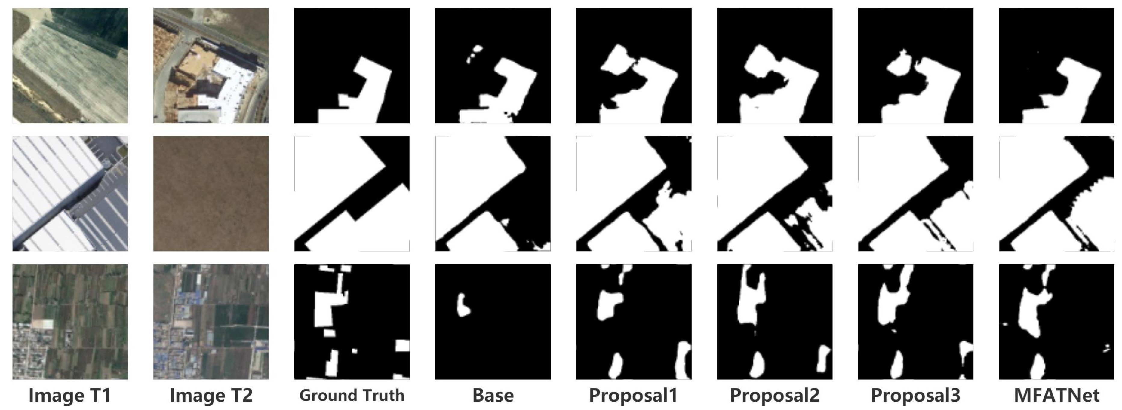
Table 1 illustrates the ablation experiments of MFATNet on three test sets, LEVIR-CD, WHU-CD, and DSIFN-CD. From this, it can be perceived that MFATNet, which integrates the three modules TM, SST, and IICAM achieves the best performance. Compared to the “Base” model, the “Proposal1” model with the TM module inserted is distinctly superior, with improvement in IoU on the three test sets, respectively. In particular, a surprising performance improvement can be observed on the DSIFN-CD dataset. Given the discussion in Section 5, such a phenomenon aptly demonstrates the robustness of the multi-scale transformer-based improvements (e.g., TM) in capturing the relationships of different relevant regions. Further, the “Proposal2” model improves the IoU by 0.3/0.64/ 2.54, respectively, compared with the “Proposal1” model, suggesting that the proposed IICAM can better smoothen the localization and semantic gaps in the feature map fusion and select a more discriminative representation. In addition, it can be noticed that the “Proposal3” model improves the IoU by 0.28/1.37/2.29 compared to the “Proposal1” model, indicating that the semantic and spatial correlation-based tokenizer improvement contributes to the performance, providing the transformer structure with better spatial context acquisition. Figure 7 depicts the schematics of the ablation studies on the LEVIR-CD, WHU-CD, and DSIFN-CD test sets.
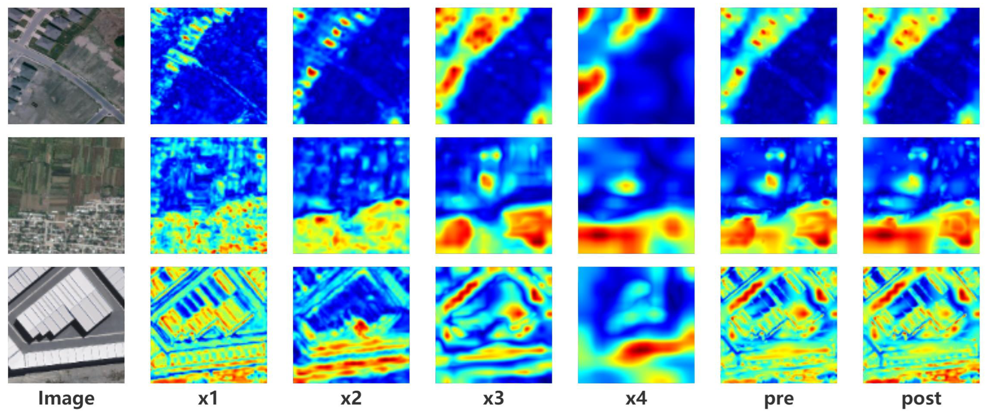
Ablation Studies on IICAM. Once the multi-scale features are extracted by the Convolutional Neural Network feature extractor and the transformer module learns the long-range dependencies, the resulting four feature maps are concatenated and passed through the final classifier to arrive at the change result map. Nevertheless, the four feature maps are subject to the removal of gaps between different channels and the selection of more discriminative representations. Thus, IICAM is introduced. IICAM is re-designed from two CAM modules that select inter-class and intra-class relationships, respectively. As mentioned in Table 2, the validity of the proposal is demonstrated by comparing the performance of using None, intra- and inter-CAM, and IICAM on Base and Proposal3. Intra-CAM suggests a CAM operation performed after summing the four feature maps along the channel dimension, while the inter-CAM performs a CAM operation after concatenating them along the channel dimension. The IICAM is a combination of both of them, and the experimental record is better than the two independent modules, as anticipated. For a clearer picture of feature fusion and the contribution of the IICAM, the four stages of feature maps, their appearance after fusion, and the introduction of the IICAM, are visualized as Figure 8.
Parameter analysis on token length. The intuition in designing the Spatial Semantic Tokenizer is to process image signals into compact word tokens as in Natural Language Processing. Thus, the length L of the token set is considered to be a crucial hyperparameter. As mentioned in Table 3, L is set to 2, 4, 8, 16, and 32, and then the experiments are conducted on the three datasets using the Proposal3 method. From the experimental results, the token length of 16 achieves the desired results on the LEVIR-CD and WHU-CD datasets, while it is 4 on the DSIFN-CD dataset. From the previous work [2,43], L of 4 [2] and 16 [43] is, respectively, adopted, with a bias toward constructing compact semantic tokens. Since the compact tokens are sufficient to specify the semantic concept of the region of interest, the redundant tokens can be detrimental to the performance of the model [2]. Meanwhile, the experimental results also illustrate this trend, both too low and too high token lengths perform worse than the intermediate value.
Ablation Studies on SST. When the feature maps from the ResNet18 extractor are obtained, they must be processed into token sets. Moreover, the region of interest must be emphasized on the token. Therefore, SST is proposed based on the Spatial Attention Module. Meanwhile, the following three tokenizer approaches are considered to demonstrate that SST is worthwhile.
- Max: Max indicates that an operation must be performed on the feature map and then flattened into a vector, .
- Avg: Avg indicates that an operation must first be performed on the feature map and then flattened into a vector, .
- ST: Semantic Tokenize (ST) indicates that point-wise convolution must be directly performed on the feature map and then transformed into tokens, without integrating SAM, compared to SST, .
The experimental results on three datasets are reported in Table 4. It can be concluded that the SST module performs better than the other three methods on the three datasets. It is considered that spatial attention simultaneously incorporates and activations, and that and are separately designed to explore the behavior of the tokenizer. At the same time, it could also be found that performs better than the other two methods, and the inference is that can preserve the overall characteristics to avoid losing more detailed representation. Instead, the proposed SST can work better in constructing compact semantic concepts, which further highlights the spatial criticality and makes the subsequent learning of the multi-scale transformer module more effective.
4.3. Comparison to Other Methods
A comparison of the proposed method is made with other existing excellent methods and the experimental results achieve promising performance. The compared methods are CNN-based methods FCEF [5], FC-Siam-D [5], FC-Siam-Conc [5] and attention-based methods DTCDSCN [14], STANet [4], IFNet [18], SNUNet [9], and the transformer-based method BiT [2].
FCEF. An image-level fusion method, which concatenates bi-temporal images by channel dimension before feeding them into an encoder–decoder architecture for convolutional networks.
FC-Siam-D. A feature-level fusion method, variants of the FCEF method, which uses a Siamese network in the feature extraction stage to extract the bi-temporal image features and then computes feature differences for fusing information.
FC-Siam-Conc. A feature-level fusion method, variants of the FCEF method, which uses a Siamese network in the feature extraction stage to extract the bi-temporal image features and then perform feature concatenate for fusing information.
DTCDSCN. An attention-based method, which introduces the auxiliary task of object extractions and dual attention module to a deep Siamese network to improve the discriminative ability of the features.
STANet. An attention-based approach, like DTCDSCN, that integrates the spatial–temporal attention mechanism into a Siamese network to determine stronger features for representation.
IFNet. A deeply supervised image fusion method in which the features are extracted at each stage by applying channel attention and spatial attention to multi-scale bi-temporal features. Deep supervision is also applied to seek results with better performance.
SNUNet. A multi-scale feature fusion method, which uses a Siamese network to fuse bi-temporal features and NestedUNet to obtain multi-scale bi-temporal features and then alleviates the gaps of different scale fusions using the channel attention module.
BIT. A transformer-based method, which uses ResNet18 to extract the feature map of a bi-temporal image, tokenize it, and then feed it into a transformer network structure to capture the long-range dependencies.
In Table 5, Table 6 and Table 7, the results of the comparison experiments on the LEVIR-CD, WHU-CD, and DSIFN-CD test sets are reported, respectively. The proposed method outperforms the other methods in terms of F1 score, IoU, and OA on all three datasets. As shown in Table 5, on the LEVIR-CD test sets, the proposed method achieved an F1 score of 90.36, IoU of 82.42, and OA of 99.03, corresponding to exceeding the second-best method BiT [2] by 1.05, 1.74, and 0.11, respectively. The proposed method also achieves competitive performance in the metrics Pre. and Rec. with 91.85 and 88.93, respectively. Table 6 presents the results for WHU-CD. An 88.31 F1 score, 79.08 IoU, and 99.01 OA are achieved, which are 0.31, 0.5, and 0.02 higher than that of BiT [2], the second-best method, respectively. As shown in Table 7, the proposed method performs best on DFISN-CD in all five metrics, while surpassing the second-best method BiT [2] in F1, IoU, and OA by 18.36, 25.01, and 6.43, respectively. It is worth noting that the proposed CNN feature extractor for MFATNet does not use sophisticated designs such as FPN [4], dense network structure [5,9,14,18], and dilated convolution [2], while the transformer further aggregates multi-scale features compared to the single-scale of BiT [2].
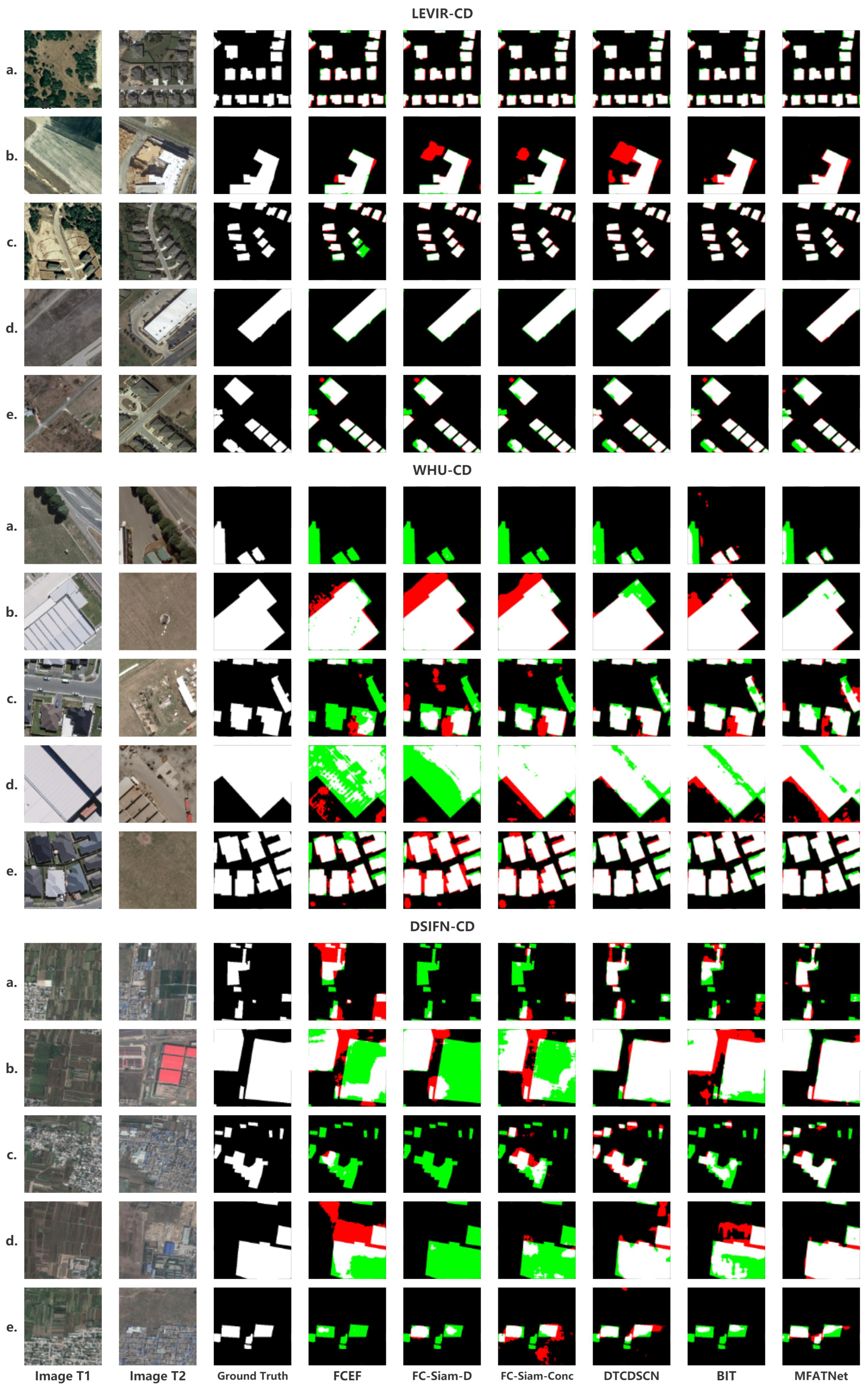
Meanwhile, it can be observed that the DSIFN-CD dataset produces a striking difference between the proposed method and the second-best method, while the boosting effect is more soothing on the other two datasets. It can also be considered that this condition is attributable to differences in the distribution of the dataset, the details of which are mentioned in Section 5. To illustrate more graphically the promising outcome of this method compared to the other methods, some of the experimental results are visualized on three datasets, as shown in Figure 9, where white denotes , black denotes , green indicates , and red denotes . The holistic visualization exhibits that the proposed method better avoids false positive and false negative (red and green account for less). At the same time, the detection of the change in the region of interest is more consistent with the ground truth in terms of appearance, and the edges of the region are processed in a better way (e.g., LEVIR-CD.a.,b.,c.,d.). It can also be noticed that the proposed method performs appreciably better than the other methods (e.g., WHU-CD.b.,d., and DSIFN-CD.b.,d.) in the face of the detection of large change regions. When large and small change regions are present concurrently, this method is also capable of addressing the two change regions with large differences at the same time (e.g., DSIFN-CD.a.,c., and WHU-CD.c.). Both the above recordings and observations suggest the proposed MFATNet has a promising effect. The visualization results for the detection of large change regions and small change regions expose the prospect of the transformer capturing long-range dependencies for remote sensing image change detection, and the performance improvement brought by the fusion between the more accurate localization information enriched by low-level visual representations and the richer semantic information embedded in high-level visual representations.
5. Discussion
In this article, we utilize the transformer to model the context of the four different scales of features generated in ResNet18, while introducing the Spatial Semantic Tokenizer (SST) for highlighting regions of interest on the token and the Intra- and Inter-class Channel Attention Module (IICAM) for alleviating the semantic and localization gaps between feature maps from different scales for a further selection of more discriminative representations when fusing multi-scale features. Compared with CNN-based methods, the proposed method has a larger effective receptive field, which is beneficial for remote sensing images where the objects of interest are widespread over all pixels of the image. For the same transformer-based change detection method, our approach leverages multi-scale features to obtain a refined change map, while further exploiting the potential of the token. However, in the actual training, we found that the utilization of the channel attention module brought a rise in the number of parameters, which is frustrating for the application of the approach to practical situations. Moreover, paper [48] mentions that the calculation of self-attention in the transformer ignores the spatial information between tokens. This is something we need to explore in our future work.
Observing the performance of each method on the above-mentioned three datasets, it can be observed that the CNN-based methods have excessive disparity in F1 score and IoU critical metrics on the LEVIR-CD dataset and DSIFN-CD dataset. For instance, the F1 score and IoU of FCEF on LEVIR-CD are 83.40 and 71.53, respectively, while the F1 value and IoU on DSIFN-CD are 61.09 and 43.98, with a difference of 22.31 and 27.55, respectively. Even for the transformer-based method, the F1 score and IoU of BiT are 20.05 and 27.71 on LEVIR-CD and DISFN-CD. The number of pixels in the changed and unchanged regions of the three datasets is counted to analyze this phenomenon, as shown in Table 8. For the LEVIR-CD dataset, the pixels in the change region of the training set accounted for 4.58 of the total pixels, whereas it was 5.09 on the test sets. On the WHU-CD dataset, the pixels in the change region of the training set accounted for 4.22 of the total pixels, while it was 4.42 on the test sets. On the DSIFN-CD dataset, the pixels in the change region of the training set accounted for 34.96 of the total pixels, whereas it was 16.99 on the test sets. The rate differences of the first two datasets are 0.51 and 0.20, respectively, while the rate difference of DSIFN-CD achieves 17.97.
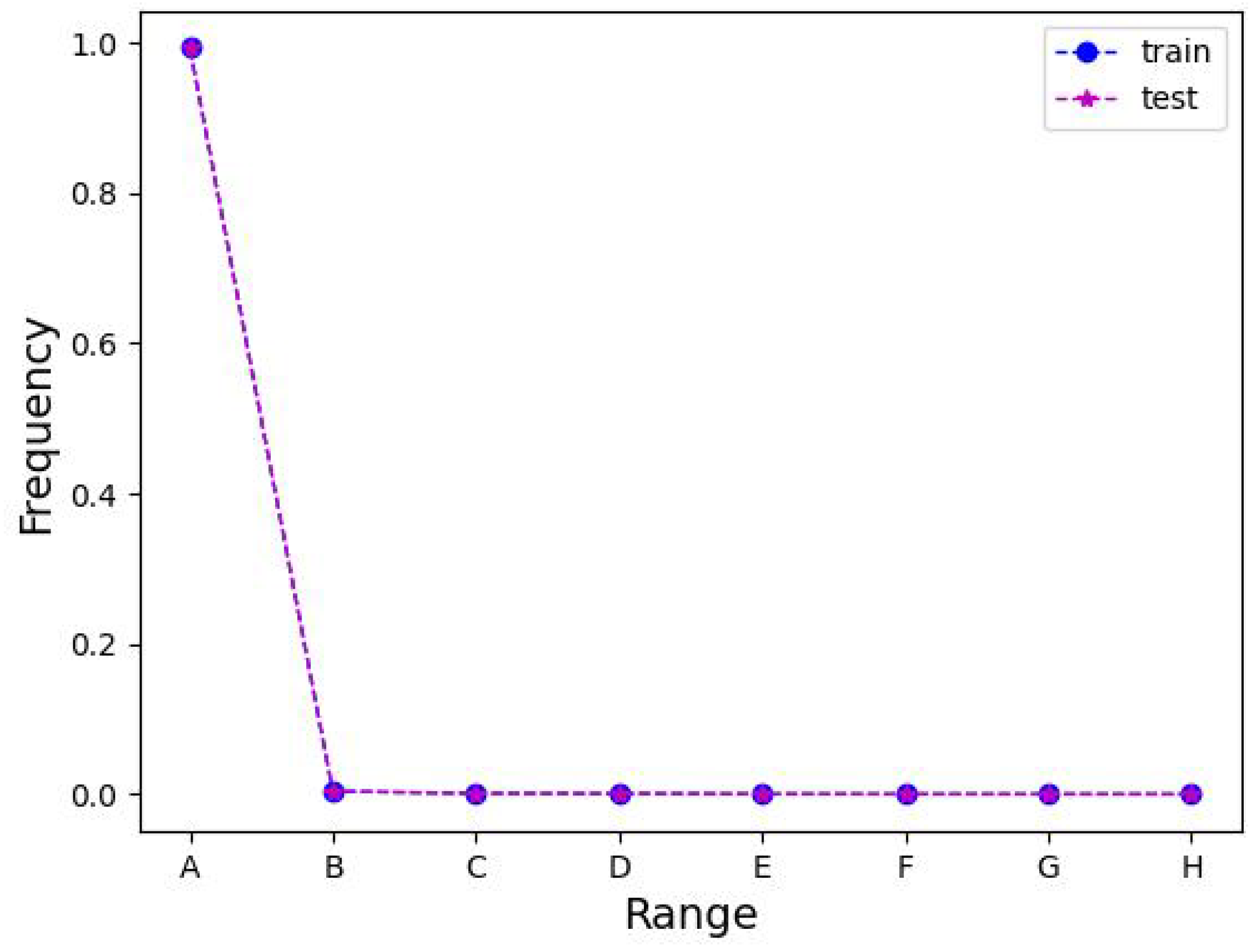
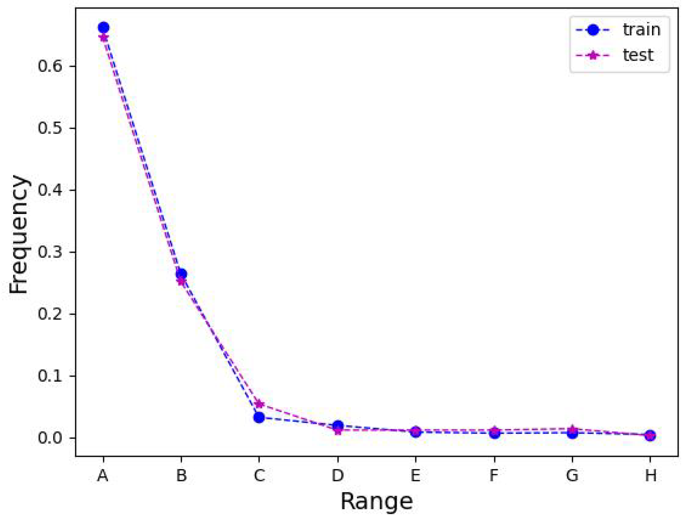
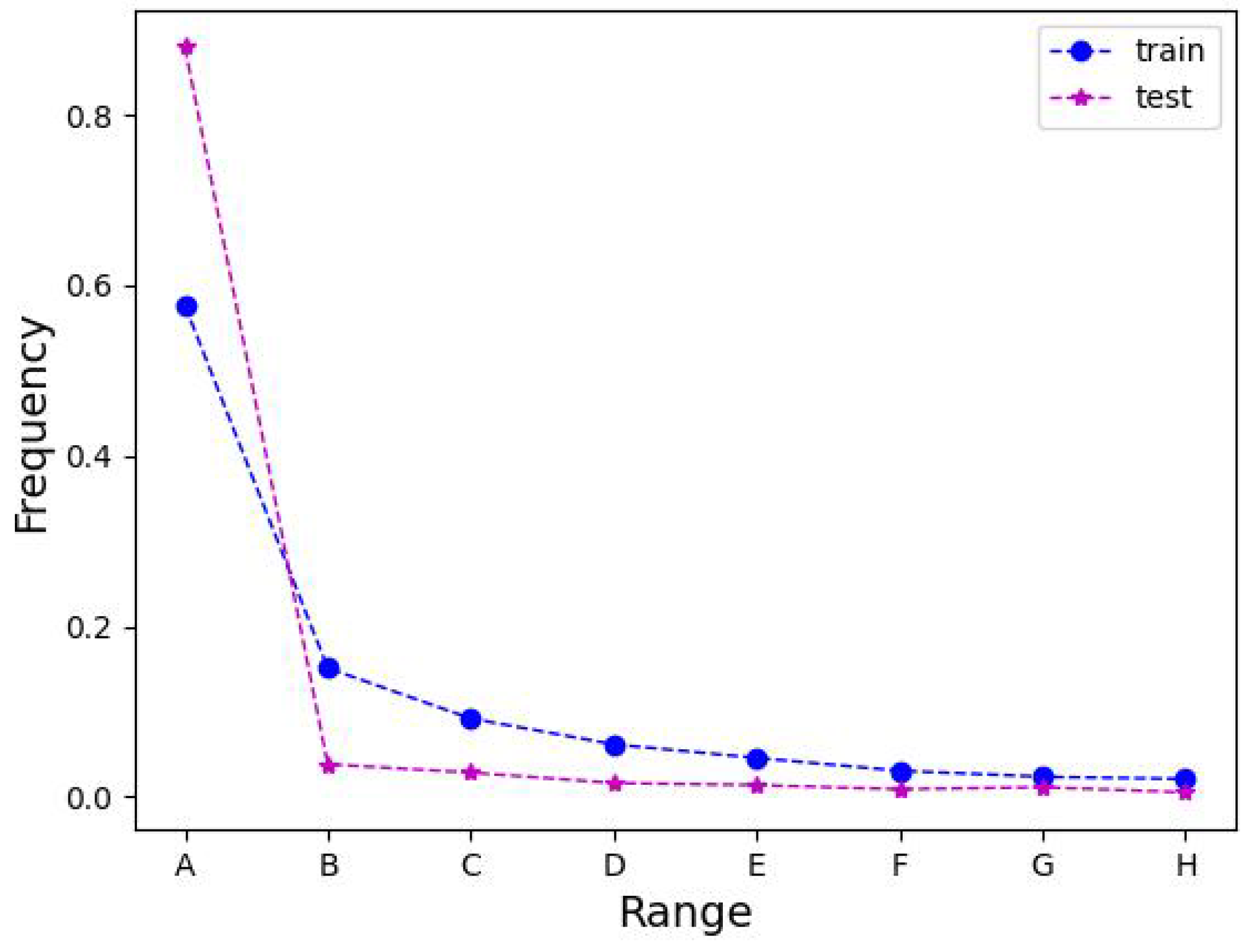
Further, the number of different area change regions is counted for the three datasets to elaborate this observation. Intuitively, it was observed that there were very few single change regions with an area share of more than half of the pixels in the image, making it reliable, as illustrated in Table 9. , and H correspond to the area ranges [0, 4096), [4096, 8192), [8192, 12288), [12,288, 16,384), [16,384, 20,480), [20,480, 24,576), [24,576, 28,672), and [28,672, 32,768), respectively. We also performed the Kolmogorov–Smirnov test on the number of different size regions of the train and test sets for the three datasets. Meanwhile, a curve chart of the percentage of different area change regions is drawn, from Figure 10, Figure 11 and Figure 12, corresponding to the LEVIR-CD, WHU-CD, and DSIFN-CD datasets, respectively. It can be observed that the curves of the training and testing sets of LEVIR-CD overlap, implying a consistent distribution, and the change regions with an area less than 4096 account for 99.3 of the total regions counted, which is friendly to the model learning. While the training and testing set curves of WHU-CD are quite close to each other, the percentage of the change regions with an area less than 4096 is 66.1 and 64.6, respectively. However, the training set and testing set curves of DSIFN have significant differences, and the percentage of change regions less than 4096 is 88.0 and 57.6, respectively, signifying a considerable difference in distribution, introducing a challenge to the generalizability and robustness of the model. Moreover, it can be observed that LEVIR-CD achieves promising accuracy on the critical F1 score and IoU due to the overwhelming advantage of the appropriate change region (e.g., A), both for CNN-based (71.53 IoU of FCEF [5]) and transformer-based (80.68 IoU of BiT [2]) methods. WHU-CD has more large change regions (e.g., B) compared to LEVIR-CD, hence more elaborate CNNs (54.49 IoU of FCEF [5] and 78.55 IoU of SNUNet [9]) are needed to improve the accuracy or use transformer-based methods (78.55 IoU of BiT [2]). However, confronted with a dataset like DSIFN-CD where the training and test sets have large differences, it is important to improve the generalization performance of the model (e.g., SST and IICAM).
Until now, it could be tentatively diagnosed that the cause of the large performance difference between the DSIFN dataset and other datasets is that the large change regions require a larger effective perceptual field, which is a natural limitation of CNN-based methods. The difference between the F1 score and IoU of the proposed MFATNet on LEVIR-CD and DSIFN-CD is 4.67 and 7.41, which significantly reduces the gap. This also depicts the favorable generalization and robustness of the proposed method.
6. Conclusions
In this study, an improved transformer-based multi-feature aggregation change detection method for remote sensing images is proposed. The proposed method extracts the features of bi-temporal images by a Siamese ResNet18 first and then converts each of the four resulting feature maps into compact semantic tokens employing a Spatial Semantic Tokenizer, which highlights the spatial relevance of the pixels in the generated token and facilitates subsequent transformer learning. The tokens are merged corresponding to different feature maps and fed into the transformer to capture the long-range dependencies between the change regions and other regions to model the spatial relationships so that a feature map with rich space–time contextual information can be obtained. After reverting the token sets and upsampling them to the original feature map dimensions, four feature maps are concatenated by the channel dimension. The rudimentary concatenation introduces localization and semantic biases, so the IICAM module is used to mitigate the gaps and select more discriminative representations. The experiments are conducted on two change detection datasets, LEVIR-CD and DSIFN-CD, and the proposed method is compared with other state-of-the-art methods. The results depict that the proposed method is more promising.
Author Contributions
Z.M. and X.T. designed the deep learning model and conducted the experiments; Z.M. wrote the paper. Z.L. and H.Z. reviewed the paper. All authors have read and agreed to the published version of the manuscript.
Funding
This work was supported in part by the Strategic Priority Research Program of the Chinese Academy of Sciences (XDA19060205, XDA19020305, and XDA19020104), in part by the Key Research Development Program of China (2019YFC0507405), and in part by the Special Project of Informatization of Chinese Academy of Sciences (CAS-WX2022GC-0106).
Data Availability Statement
Our code will be available at https://github.com/maozan/mfatnet.
Conflicts of Interest
The authors declare no conflict of interest.
References
- Singh, A. Review article digital change detection techniques using remotely-sensed data. Int. J. Remote Sens. 1989, 10, 989–1003. [Google Scholar] [CrossRef] [Green Version]
- Chen, H.; Qi, Z.; Shi, Z. Remote sensing image change detection with transformers. IEEE Trans. Geosci. Remote Sens. 2021, 60, 1–14. [Google Scholar] [CrossRef]
- Bandara, W.G.C.; Patel, V.M. A transformer-based siamese network for change detection. arXiv 2022, arXiv:2201.01293. [Google Scholar]
- Chen, H.; Shi, Z. A Spatial-Temporal Attention-Based Method and a New Dataset for Remote Sensing Image Change Detection. Remote Sens. 2020, 12, 1662. [Google Scholar] [CrossRef]
- Daudt, R.C.; Le Saux, B.; Boulch, A. Fully convolutional siamese networks for change detection. In Proceedings of the 2018 25th IEEE International Conference on Image Processing (ICIP), Athens, Greece, 7–10 October 2018; pp. 4063–4067. [Google Scholar]
- Shi, W.; Zhang, M.; Zhang, R.; Chen, S.; Zhan, Z. Change Detection Based on Artificial Intelligence: State-of-the-Art and Challenges. Remote Sens. 2020, 12, 1688. [Google Scholar] [CrossRef]
- Song, F.; Zhang, S.; Lei, T.; Song, Y.; Peng, Z. MSTDSNet-CD: Multi-scale Swin Transformer and Deeply Supervised Network for Change Detection of the Fast-Growing Urban Regions. IEEE Geosci. Remote Sens. Lett. 2022, 19, 1–5. [Google Scholar] [CrossRef]
- Daudt, R.C.; Le Saux, B.; Boulch, A.; Gousseau, Y. Urban change detection for multispectral earth observation using Convolutional Neural Networks. In Proceedings of the IGARSS 2018-2018 IEEE International Geoscience and Remote Sensing Symposium, Valencia, Spain, 22–27 July 2018; pp. 2115–2118. [Google Scholar]
- Fang, S.; Li, K.; Shao, J.; Li, Z. SNUNet-CD: A densely connected siamese network for change detection of VHR images. IEEE Geosci. Remote Sens. Lett. 2021, 19, 1–5. [Google Scholar] [CrossRef]
- Chen, H.; Li, W.; Shi, Z. Adversarial Instance Augmentation for Building Change Detection in Remote Sensing Images. IEEE Trans. Geosci. Remote Sens. 2021, 60, 1–16. [Google Scholar] [CrossRef]
- Peng, D.; Bruzzone, L.; Zhang, Y.; Guan, H.; Ding, H.; Huang, X. SemiCDNet: A semisupervised Convolutional Neural Network for change detection in high resolution remote-sensing images. IEEE Trans. Geosci. Remote Sens. 2020, 59, 5891–5906. [Google Scholar] [CrossRef]
- Chen, J.; Yuan, Z.; Peng, J.; Chen, L.; Huang, H.; Zhu, J.; Liu, Y.; Li, H. DASNet: Dual attentive fully convolutional siamese networks for change detection in high-resolution satellite images. IEEE J. Sel. Top. Appl. Earth Obs. Remote Sens. 2020, 14, 1194–1206. [Google Scholar] [CrossRef]
- Ji, S.; Wei, S.; Lu, M. Fully convolutional networks for multisource building extraction from an open aerial and satellite imagery data set. IEEE Trans. Geosci. Remote Sens. 2018, 57, 574–586. [Google Scholar] [CrossRef]
- Liu, Y.; Pang, C.; Zhan, Z.; Zhang, X.; Yang, X. Building change detection for remote sensing images using a dual-task constrained deep siamese convolutional network model. IEEE Geosci. Remote Sens. Lett. 2020, 18, 811–815. [Google Scholar] [CrossRef]
- Long, J.; Shelhamer, E.; Darrell, T. Fully Convolutional Networks for Semantic Segmentation. IEEE Trans. Pattern Anal. Mach. Intell. 2015, 39, 640–651. [Google Scholar]
- Ronneberger, O.; Fischer, P.; Brox, T. U-Net: Convolutional Networks for Biomedical Image Segmentation; Springer International Publishing: Berlin/Heidelberg, Germany, 2015. [Google Scholar]
- Peng, D.; Zhang, Y.; Guan, H. End-to-end change detection for high resolution satellite images using improved UNet++. Remote Sens. 2019, 11, 1382. [Google Scholar] [CrossRef] [Green Version]
- Zhang, C.; Yue, P.; Tapete, D.; Jiang, L.; Shangguan, B.; Huang, L.; Liu, G. A deeply supervised image fusion network for change detection in high resolution bi-temporal remote sensing images. ISPRS J. Photogramm. Remote Sens. 2020, 166, 183–200. [Google Scholar] [CrossRef]
- Zhang, M.; Xu, G.; Chen, K.; Yan, M.; Sun, X. Triplet-based semantic relation learning for aerial remote sensing image change detection. IEEE Geosci. Remote Sens. Lett. 2018, 16, 266–270. [Google Scholar] [CrossRef]
- Zhang, M.; Shi, W. A feature difference Convolutional Neural Network-based change detection method. IEEE Trans. Geosci. Remote Sens. 2020, 58, 7232–7246. [Google Scholar] [CrossRef]
- Dosovitskiy, A.; Beyer, L.; Kolesnikov, A.; Weissenborn, D.; Zhai, X.; Unterthiner, T.; Dehghani, M.; Minderer, M.; Heigold, G.; Gelly, S.; et al. An image is worth 16x16 words: Transformers for image recognition at scale. arXiv 2020, arXiv:2010.11929. [Google Scholar]
- Liu, Z.; Lin, Y.; Cao, Y.; Hu, H.; Wei, Y.; Zhang, Z.; Lin, S.; Guo, B. Swin transformer: Hierarchical vision transformer using shifted windows. In Proceedings of the IEEE/CVF International Conference on Computer Vision, Montreal, QC, Canada, 10–17 October 2021; pp. 10012–10022. [Google Scholar]
- Wang, W.; Xie, E.; Li, X.; Fan, D.P.; Song, K.; Liang, D.; Lu, T.; Luo, P.; Shao, L. Pyramid vision transformer: A versatile backbone for dense prediction without convolutions. In Proceedings of the IEEE/CVF International Conference on Computer Vision, Montreal, QC, Canada, 10–17 October 2021; pp. 568–578. [Google Scholar]
- Ke, Q.; Zhang, P. Hybrid-TransCD: A Hybrid Transformer Remote Sensing Image Change Detection Network via Token Aggregation. ISPRS Int. J. Geo-Inf. 2022, 11, 263. [Google Scholar] [CrossRef]
- Lin, T.Y.; Dollár, P.; Girshick, R.; He, K.; Hariharan, B.; Belongie, S. Feature Pyramid Networks for object detection. In Proceedings of the IEEE Conference on Computer Vision and Pattern Recognition, Honolulu, HI, USA, 21–26 July 2017; pp. 2117–2125. [Google Scholar]
- He, K.; Zhang, X.; Ren, S.; Sun, J. Deep residual learning for image recognition. In Proceedings of the IEEE Conference on Computer Vision and Pattern Recognition, Las Vegas, NV, USA, 27–30 June 2016; pp. 770–778. [Google Scholar]
- Nemoto, K.; Hamaguchi, R.; Sato, M.; Fujita, A.; Imaizumi, T.; Hikosaka, S. Building change detection via a combination of CNNs using only RGB aerial imageries. In Proceedings of the Remote Sensing Technologies and Applications in Urban Environments II, Warsaw, Poland, 11–12 September 2017; Volume 10431, pp. 107–118. [Google Scholar]
- Ji, S.; Shen, Y.; Lu, M.; Zhang, Y. Building instance change detection from large-scale aerial images using Convolutional Neural Networks and simulated samples. Remote Sens. 2019, 11, 1343. [Google Scholar] [CrossRef] [Green Version]
- Liu, R.; Kuffer, M.; Persello, C. The temporal dynamics of slums employing a CNN-based change detection approach. Remote Sens. 2019, 11, 2844. [Google Scholar] [CrossRef] [Green Version]
- Rahman, F.; Vasu, B.; Van Cor, J.; Kerekes, J.; Savakis, A. Siamese network with multi-level features for patch-based change detection in satellite imagery. In Proceedings of the 2018 IEEE Global Conference on Signal and Information Processing (GlobalSIP), Anaheim, CA, USA, 26–29 November 2018; pp. 958–962. [Google Scholar]
- Zhou, Z.; Rahman Siddiquee, M.M.; Tajbakhsh, N.; Liang, J. Unet++: A nested u-net architecture for medical image segmentation. In Deep Learning in Medical Image Analysis and Multimodal Learning for Clinical Decision Support; Springer: Berlin/Heidelberg, Germany, 2018; pp. 3–11. [Google Scholar]
- Chen, L.C.; Zhu, Y.; Papandreou, G.; Schroff, F.; Adam, H. Encoder-Decoder with Atrous Separable Convolution for Semantic Image Segmentation; Springer: Berlin/Heidelberg, Germany, 2018. [Google Scholar]
- Bem, P.P.D.; Júnior, O.; Guimares, R.F.; Gomes, R. Change Detection of Deforestation in the Brazilian Amazon Using Landsat Data and Convolutional Neural Networks. Remote Sens. 2020, 12, 901. [Google Scholar] [CrossRef] [Green Version]
- Bao, T.; Fu, C.; Fang, T.; Huo, H. PPCNET: A combined patch-level and pixel-level end-to-end deep network for high-resolution remote sensing image change detection. IEEE Geosci. Remote Sens. Lett. 2020, 17, 1797–1801. [Google Scholar] [CrossRef]
- Diakogiannis, F.I.; Waldner, F.; Caccetta, P. Looking for change? Roll the Dice and demand Attention. Remote Sens. 2021, 13, 3707. [Google Scholar] [CrossRef]
- Fang, B.; Pan, L.; Kou, R. Dual learning-based siamese framework for change detection using bi-temporal VHR optical remote sensing images. Remote Sens. 2019, 11, 1292. [Google Scholar] [CrossRef] [Green Version]
- Hou, B.; Liu, Q.; Wang, H.; Wang, Y. From W-Net to CDGAN: Bitemporal change detection via deep learning techniques. IEEE Trans. Geosci. Remote Sens. 2019, 58, 1790–1802. [Google Scholar] [CrossRef] [Green Version]
- Jiang, H.; Hu, X.; Li, K.; Zhang, J.; Gong, J.; Zhang, M. PGA-SiamNet: Pyramid feature-based attention-guided siamese network for remote sensing orthoimagery building change detection. Remote Sens. 2020, 12, 484. [Google Scholar] [CrossRef] [Green Version]
- Peng, X.; Zhong, R.; Li, Z.; Li, Q. Optical remote sensing image change detection based on attention mechanism and image difference. IEEE Trans. Geosci. Remote Sens. 2020, 59, 7296–7307. [Google Scholar] [CrossRef]
- Lebedev, M.; Vizilter, Y.V.; Vygolov, O.; Knyaz, V.; Rubis, A.Y. Change detection in remote sensing images using conditional adversarial networks. Int. Arch. Photogramm. Remote Sens. Spat. Inf. Sci. 2018, 42, 565–571. [Google Scholar] [CrossRef] [Green Version]
- Zhao, W.; Chen, X.; Ge, X.; Chen, J. Using adversarial network for multiple change detection in bitemporal remote sensing imagery. IEEE Geosci. Remote Sens. Lett. 2020, 19, 8003605. [Google Scholar] [CrossRef]
- Zhan, Y.; Fu, K.; Yan, M.; Sun, X.; Wang, H.; Qiu, X. Change detection based on deep siamese convolutional network for optical aerial images. IEEE Geosci. Remote Sens. Lett. 2017, 14, 1845–1849. [Google Scholar] [CrossRef]
- Wu, B.; Xu, C.; Dai, X.; Wan, A.; Zhang, P.; Yan, Z.; Tomizuka, M.; Gonzalez, J.; Keutzer, K.; Vajda, P. Visual transformers: Token-based image representation and processing for computer vision. arXiv 2020, arXiv:2006.03677. [Google Scholar]
- Zheng, S.; Lu, J.; Zhao, H.; Zhu, X.; Luo, Z.; Wang, Y.; Fu, Y.; Feng, J.; Xiang, T.; Torr, P.H.; et al. Rethinking semantic segmentation from a sequence-to-sequence perspective with transformers. In Proceedings of the IEEE/CVF Conference on Computer Vision and Pattern Recognition, Montreal, QC, Canada, 10–17 October 2021; pp. 6881–6890. [Google Scholar]
- Xie, E.; Wang, W.; Yu, Z.; Anandkumar, A.; Alvarez, J.M.; Luo, P. SegFormer: Simple and efficient design for semantic segmentation with transformers. Adv. Neural Inf. Process. Syst. 2021, 34, 12077–12090. [Google Scholar]
- Zhang, D.; Zhang, H.; Tang, J.; Wang, M.; Hua, X.; Sun, Q. Feature pyramid transformer. In Proceedings of the European Conference on Computer Vision, Glasgow, UK, 23–28 August 2020; Springer: Berlin/Heidelberg, Germany, 2020; pp. 323–339. [Google Scholar]
- Hendrycks, D.; Gimpel, K. Gaussian error linear units (gelus). arXiv 2016, arXiv:1606.08415. [Google Scholar]
- Gao, L.; Liu, H.; Yang, M.; Chen, L.; Wan, Y.; Xiao, Z.; Qian, Y. STransFuse: Fusing swin transformer and Convolutional Neural Network for remote sensing image semantic segmentation. IEEE J. Sel. Top. Appl. Earth Obs. Remote Sens. 2021, 14, 10990–11003. [Google Scholar] [CrossRef]
Figure 1.
The diagram of the different fusion methods, image-level fusion (left) and feature-level fusion (right). The dark yellow square indicates the fusion method and the resulting Change Map (CM).
Figure 1.
The diagram of the different fusion methods, image-level fusion (left) and feature-level fusion (right). The dark yellow square indicates the fusion method and the resulting Change Map (CM).

Figure 2.
The diagram of the proposed MFATNet. The bi-temporal remote sensing images are fed into a Siamese ResNet18, which obtains two sets of feature maps for each of the last four stages. The feature maps are then fed into the transformer module to learn long-range dependencies after being processed into compact semantic tokens by the SST module. The context-rich tokens are then mapped and upsampled to the raw size, and the resulting change map is obtained by the IICAM module after eliminating the gaps and further choosing more discriminative representations.

Figure 3.
The diagram of the Spatial Semantic Tokenizer.

Figure 4.
The diagram of the multi-tokens.

Figure 5.
The diagram of the transformer structure.

Figure 6.
The diagram of the Intra- and Inter-class Channel Attention Module.

Figure 7.
From top to bottom once are comparative figures of the LEVIR-CD, WHU-CD, and DSIFN-CD datasets regarding MFATNet ablation experiments. As with Table 1, “MFATNet” is a better visualization than “Base”, “Proposal1”, “Proposal2”, and “Proposal3”.
Figure 7.
From top to bottom once are comparative figures of the LEVIR-CD, WHU-CD, and DSIFN-CD datasets regarding MFATNet ablation experiments. As with Table 1, “MFATNet” is a better visualization than “Base”, “Proposal1”, “Proposal2”, and “Proposal3”.

Figure 8.
The diagram of the four stages of the feature map and their integration. xi denotes the four-stage feature map, pre indicates fusion that utilizes IICAM previously, and post denotes fusion that utilizes IICAM post. Red represents the semantics of the object; blue represents irrelevant objects and fills in the boundaries of the object.

Figure 9.
The visualization results of the different methods on the test sets of the three datasets (a–e); black represents , white represents , red represents , and green represents .
Figure 9.
The visualization results of the different methods on the test sets of the three datasets (a–e); black represents , white represents , red represents , and green represents .

Figure 10.
The folding chart of the percentage of different regions in the LEVIR-CD dataset.

Figure 11.
The folding chart of the percentage of different regions in the WHU-CD dataset.

Figure 12.
The folding chart of the percentage of different regions in the DSIFN-CD dataset.


Table 1.
Ablation studies of MFATNet on the test sets of LEVIR-CD, WHU-CD, and DSIFN-CD.
| Method | TM. | SST. | IICAM. | LEVIR-CD | WHU-CD | DSIFN-CD | |||
|---|---|---|---|---|---|---|---|---|---|
| F1 | IoU | F1 | IoU | F1 | IoU | ||||
| Base | - | - | - | 88.46 | 79.31 | 86.10 | 75.59 | 69.08 | 52.77 |
| Proposal1 | √ | - | - | 90.12 | 82.02 | 86.41 | 76.07 | 84.89 | 73.75 |
| Proposal2 | √ | - | √ | 90.30 | 82.32 | 86.82 | 76.71 | 86.54 | 76.29 |
| Proposal3 | √ | √ | - | 90.29 | 82.30 | 87.29 | 77.44 | 86.79 | 76.67 |
| MFATNet | √ | √ | √ | 90.36 | 82.42 | 88.31 | 79.08 | 87.62 | 77.98 |
Table 2.
Ablation studies of IICAM on three test sets.
| Method | LEVIR-CD | WHU-CD | DSIFN-CD | |||
|---|---|---|---|---|---|---|
| F1 | IoU | F1 | IoU | F1 | IoU | |
| Proposal3 | 90.29 | 82.30 | 87.29 | 77.44 | 86.79 | 76.67 |
| Proposal3 + intra-CAM | 90.16 | 82.08 | 87.65 | 78.02 | 87.59 | 77.93 |
| Proposal3 + inter-CAM | 90.33 | 82.38 | 87.67 | 78.05 | 87.47 | 77.73 |
| Proposal3 + IICAM | 90.36 | 82.42 | 88.31 | 79.08 | 87.62 | 77.98 |
Table 3.
The experimental results of parameter analysis on tokens length.
| L | LEVIR-CD | WHU-CD | DSIFN-CD | |||
|---|---|---|---|---|---|---|
| F1 | IoU | F1 | IoU | F1 | IoU | |
| 2 | 89.93 | 81.70 | 85.89 | 75.26 | 86.50 | 76.22 |
| 4 | 89.90 | 81.65 | 86.87 | 76.79 | 86.79 | 76.67 |
| 8 | 89.87 | 81.61 | 86.40 | 76.06 | 85.31 | 74.39 |
| 16 | 89.94 | 81.72 | 87.29 | 77.44 | 86.58 | 76.33 |
| 32 | 89.93 | 81.70 | 86.41 | 76.07 | 86.57 | 76.33 |
Table 4.
Ablation studies of SST on three test sets.
| Method | LEVIR-CD | WHU-CD | DSIFN-CD | |||
|---|---|---|---|---|---|---|
| F1 | IoU | F1 | IoU | F1 | IoU | |
| Max | 90.12 | 82.02 | 85.33 | 74.72 | 84.89 | 73.75 |
| Avg | 90.26 | 82.25 | 86.82 | 76.71 | 86.15 | 75.67 |
| ST | 90.21 | 82.16 | 86.23 | 75.79 | 85.62 | 74.85 |
| SST | 90.29 | 82.30 | 88.31 | 79.08 | 87.62 | 77.98 |
Table 5.
The experimental results on the LEVIR-CD test sets *.
| Method | Pre. | Rec. | F1 | IoU | OA |
|---|---|---|---|---|---|
| FCEF | 86.91 | 80.17 | 83.40 | 71.53 | 98.39 |
| FC-Siam-D | 89.53 | 83.31 | 86.31 | 75.92 | 98.67 |
| FC-Siam-Conc | 91.99 | 76.77 | 83.69 | 71.96 | 98.49 |
| DTCDSCN | 88.53 | 86.83 | 87.67 | 78.05 | 98.77 |
| STANet | 83.81 | 91.00 | 87.26 | 77.40 | 98.66 |
| IFNet | 94.02 | 82.93 | 88.13 | 78.77 | 98.87 |
| SNUNet | 89.18 | 87.17 | 88.16 | 78.83 | 98.82 |
| BIT | 89.24 | 89.37 | 89.31 | 80.68 | 98.92 |
| Ours | 91.85 | 88.93 | 90.36 | 82.42 | 99.03 |
* Color escription: best, 2nd-best, and 3rd-best.
Table 6.
The experimental results on the WHU-CD test sets *.
| Method | Pre. | Rec. | F1 | IoU | OA |
|---|---|---|---|---|---|
| FCEF | 81.12 | 62.40 | 70.54 | 54.49 | 97.69 |
| FC-Siam-D | 80.28 | 73.59 | 76.79 | 62.32 | 98.03 |
| FC-Siam-Conc | 82.07 | 75.26 | 78.52 | 64.63 | 98.17 |
| DTCDSCN | 94.42 | 80.99 | 87.20 | 77.30 | 98.94 |
| SNUNet | 92.01 | 84.30 | 87.99 | 78.55 | 98.98 |
| BIT | 93.48 | 83.13 | 88.00 | 78.58 | 98.99 |
| Ours | 93.18 | 83.93 | 88.31 | 79.08 | 99.01 |
* Color escription: best, 2nd-best, and 3rd-best.
Table 7.
The experimental results on the DSIFN-CD test sets *.
| Method | Pre. | Rec. | F1 | IoU | OA |
|---|---|---|---|---|---|
| FCEF | 72.61 | 52.73 | 61.09 | 43.98 | 88.59 |
| FC-Siam-D | 59.67 | 65.71 | 62.54 | 45.50 | 86.63 |
| FC-Siam-Conc | 66.45 | 54.21 | 59.71 | 42.56 | 87.57 |
| DTCDSCN | 53.87 | 77.99 | 63.72 | 46.76 | 84.91 |
| STANet | 67.71 | 61.68 | 64.56 | 47.66 | 88.49 |
| IFNet | 67.86 | 53.94 | 60.10 | 42.96 | 87.83 |
| SNUNet | 60.60 | 72.89 | 66.18 | 49.45 | 87.34 |
| BIT | 68.36 | 70.18 | 69.26 | 52.97 | 89.41 |
| Ours | 88.65 | 86.62 | 87.62 | 77.98 | 95.84 |
* Color escription: best, 2nd-best, and 3rd-best.
Table 8.
The number of pixels in the change area on the three datasets.
| Dataset | Train Sets | Test Sets | ||||
|---|---|---|---|---|---|---|
| Change | Total | Rate (%) | Change | Total | Rate (%) | |
| LEVIR | 21,412,341 | 466,616,320 | 4.58% | 6,837,335 | 134,217,728 | 5.09% |
| WHU | 16,885,897 | 399,507,456 | 4.22% | 2,210,480 | 49,938,432 | 4.42% |
| DSIFN | 330,013,136 | 943,718,400 | 34.96% | 2,138,110 | 12,582,912 | 16.99% |
Table 9.
The statistics of the number of regions with different size change in the three datasets.
| Range | LEVIR | WHU | DSIFN | |||
|---|---|---|---|---|---|---|
| Train | Test | Train | Test | Train | Test | |
| A | 26,424 | 8613 | 2506 | 291 | 15,483 | 720 |
| B | 103 | 37 | 999 | 113 | 4049 | 31 |
| C | 31 | 5 | 120 | 24 | 2460 | 23 |
| D | 19 | 9 | 71 | 5 | 1645 | 13 |
| E | 4 | 5 | 30 | 5 | 1216 | 11 |
| F | 6 | 1 | 23 | 5 | 814 | 7 |
| G | 6 | 0 | 26 | 6 | 624 | 9 |
| H | 2 | 1 | 15 | 1 | 554 | 4 |
| * | ||||||
| * | ||||||
* isnorm denotes whether to obey the normal distribution, and issame denotes whether to obey the same distribution.
Publisher’s Note: MDPI stays neutral with regard to jurisdictional claims in published maps and institutional affiliations. |
© 2022 by the authors. Licensee MDPI, Basel, Switzerland. This article is an open access article distributed under the terms and conditions of the Creative Commons Attribution (CC BY) license (https://creativecommons.org/licenses/by/4.0/).
Share and Cite
MDPI and ACS Style
Mao, Z.; Tong, X.; Luo, Z.; Zhang, H. MFATNet: Multi-Scale Feature Aggregation via Transformer for Remote Sensing Image Change Detection. Remote Sens. 2022, 14, 5379. https://doi.org/10.3390/rs14215379
AMA Style
Mao Z, Tong X, Luo Z, Zhang H. MFATNet: Multi-Scale Feature Aggregation via Transformer for Remote Sensing Image Change Detection. Remote Sensing. 2022; 14(21):5379. https://doi.org/10.3390/rs14215379
Chicago/Turabian StyleMao, Zan, Xinyu Tong, Ze Luo, and Honghai Zhang. 2022. "MFATNet: Multi-Scale Feature Aggregation via Transformer for Remote Sensing Image Change Detection" Remote Sensing 14, no. 21: 5379. https://doi.org/10.3390/rs14215379
Note that from the first issue of 2016, this journal uses article numbers instead of page numbers. See further details here.