


Refinement of Individual Tree Detection Results Obtained from Airborne Laser Scanning Data for a Mixed Natural Forest
 ,
,  , , ,
, , ,
Abstract
:1. Introduction
2. Materials
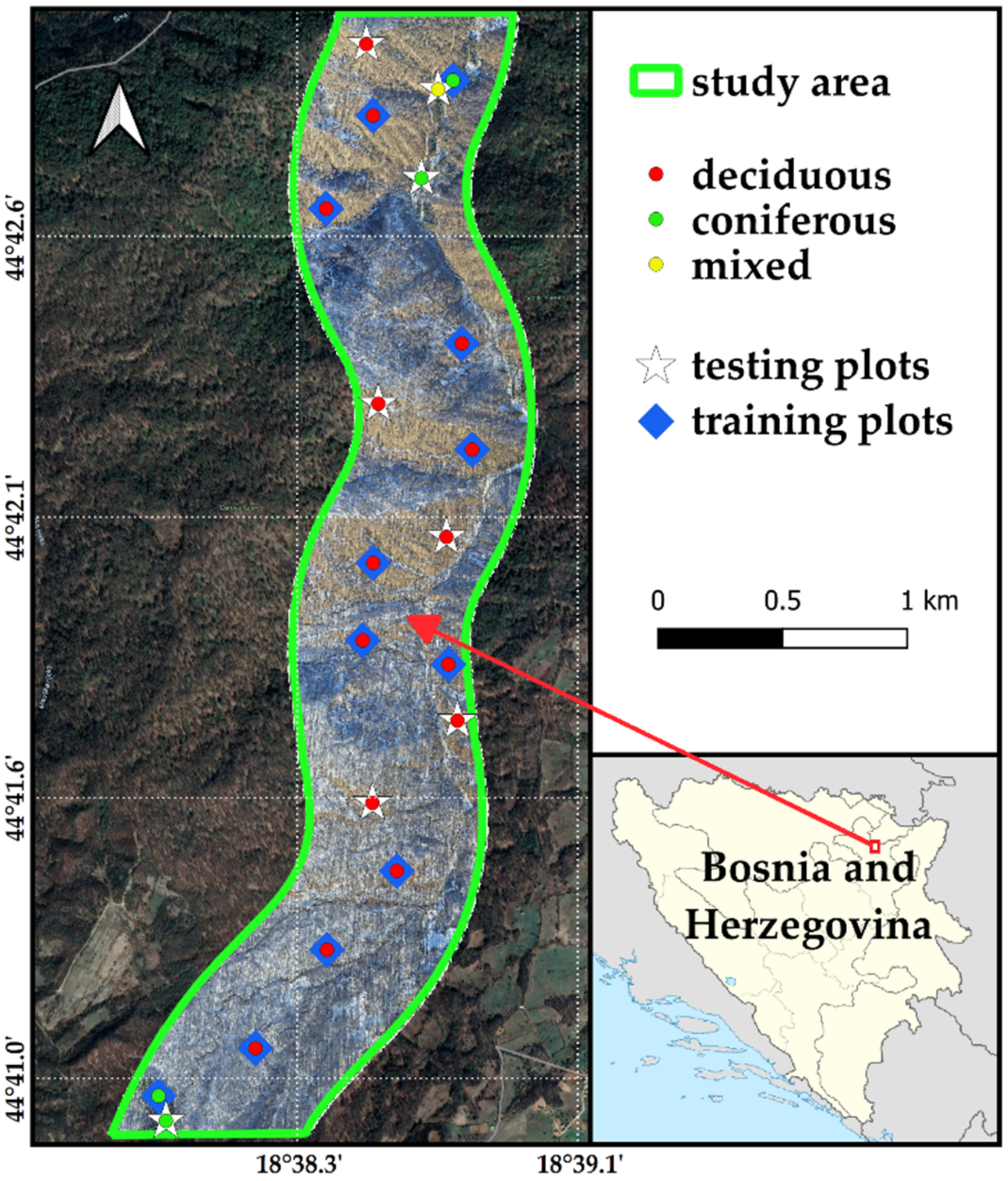
2.1. Study Area
2.2. Forest Plots
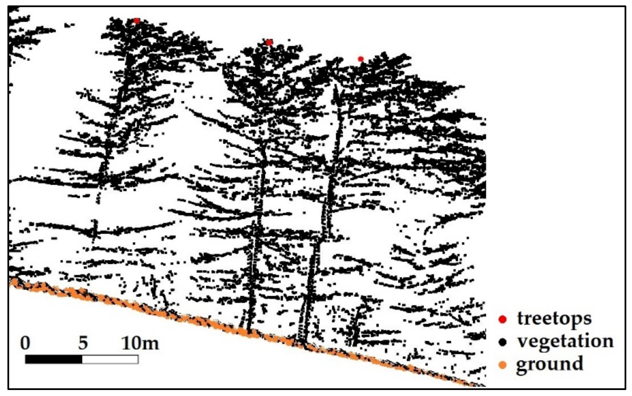
2.3. ALS Data
2.4. Reference Tree Data
3. Methods
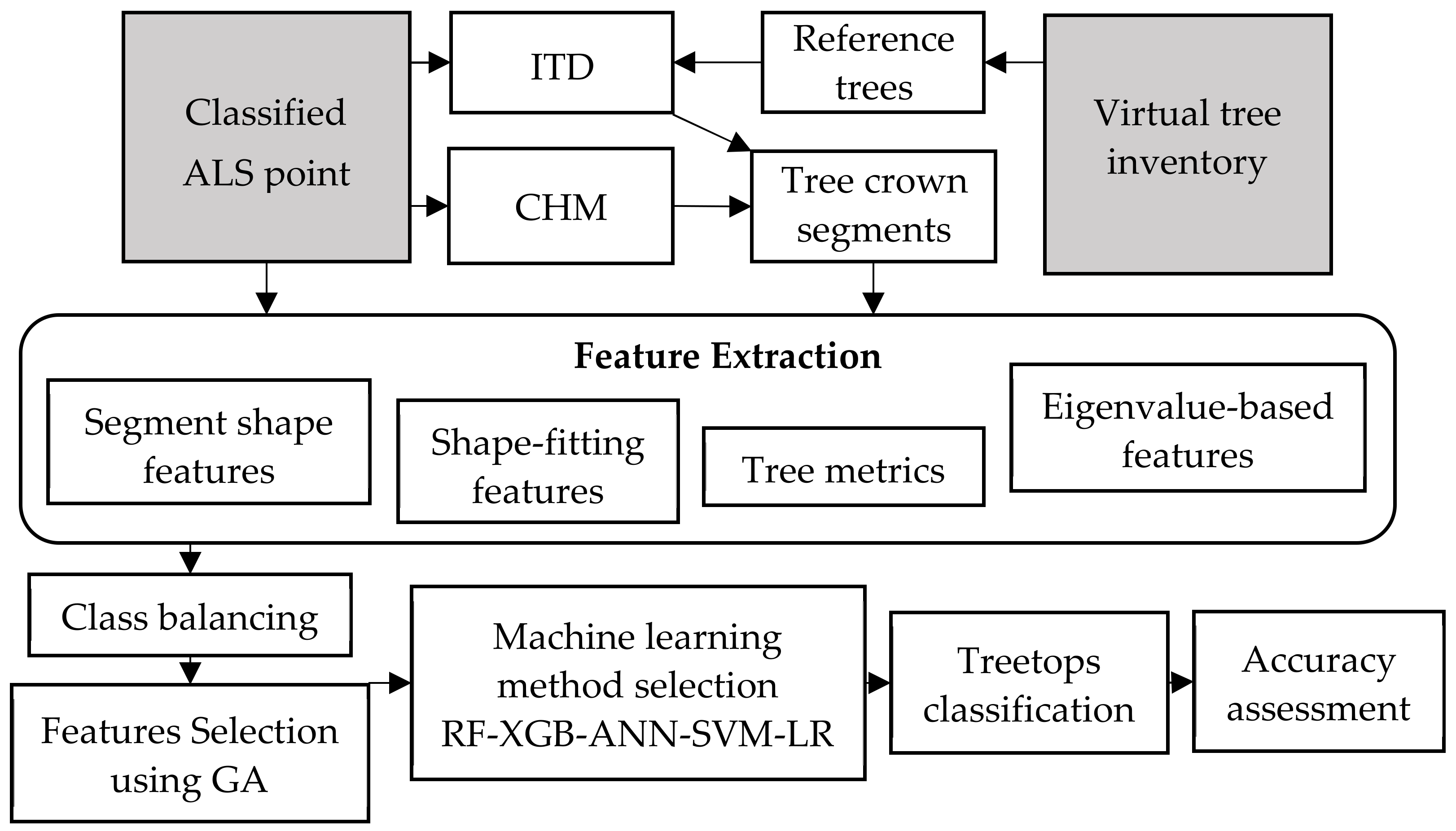
3.1. Methodology
3.2. CHM Generation, ITD and Tree Crown Segmentation
3.3. Feature Extraction
3.3.1. Tree Metrics
3.3.2. Segment Shape Features
3.3.3. Eigenvalue-Based Features
3.3.4. Shape-Fitting Features
3.4. Data Balancing and Feature Selection
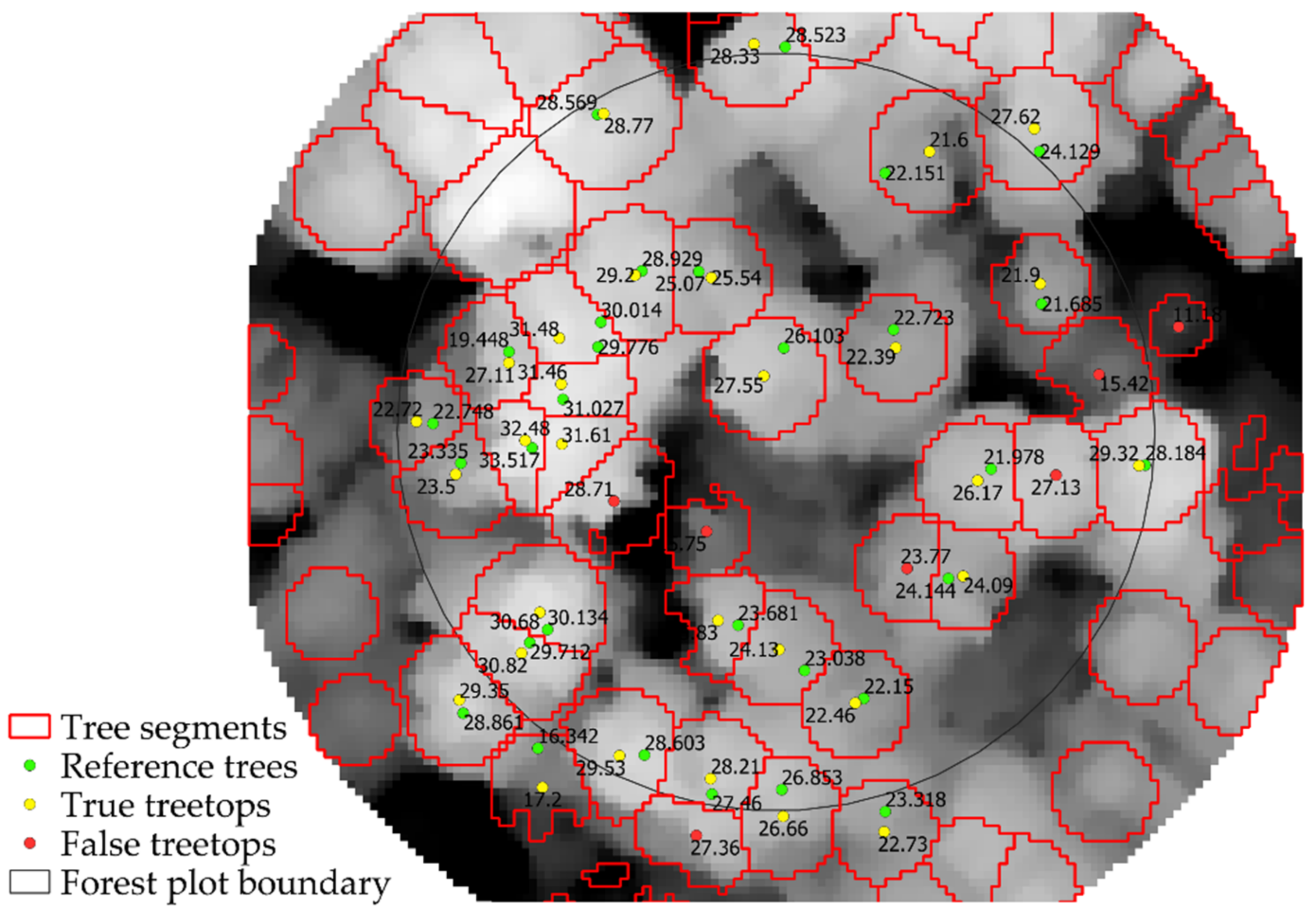
3.5. Treetops Class Labelling
3.6. Classification Method Selection
3.7. Accuracy Assessment
4. Results
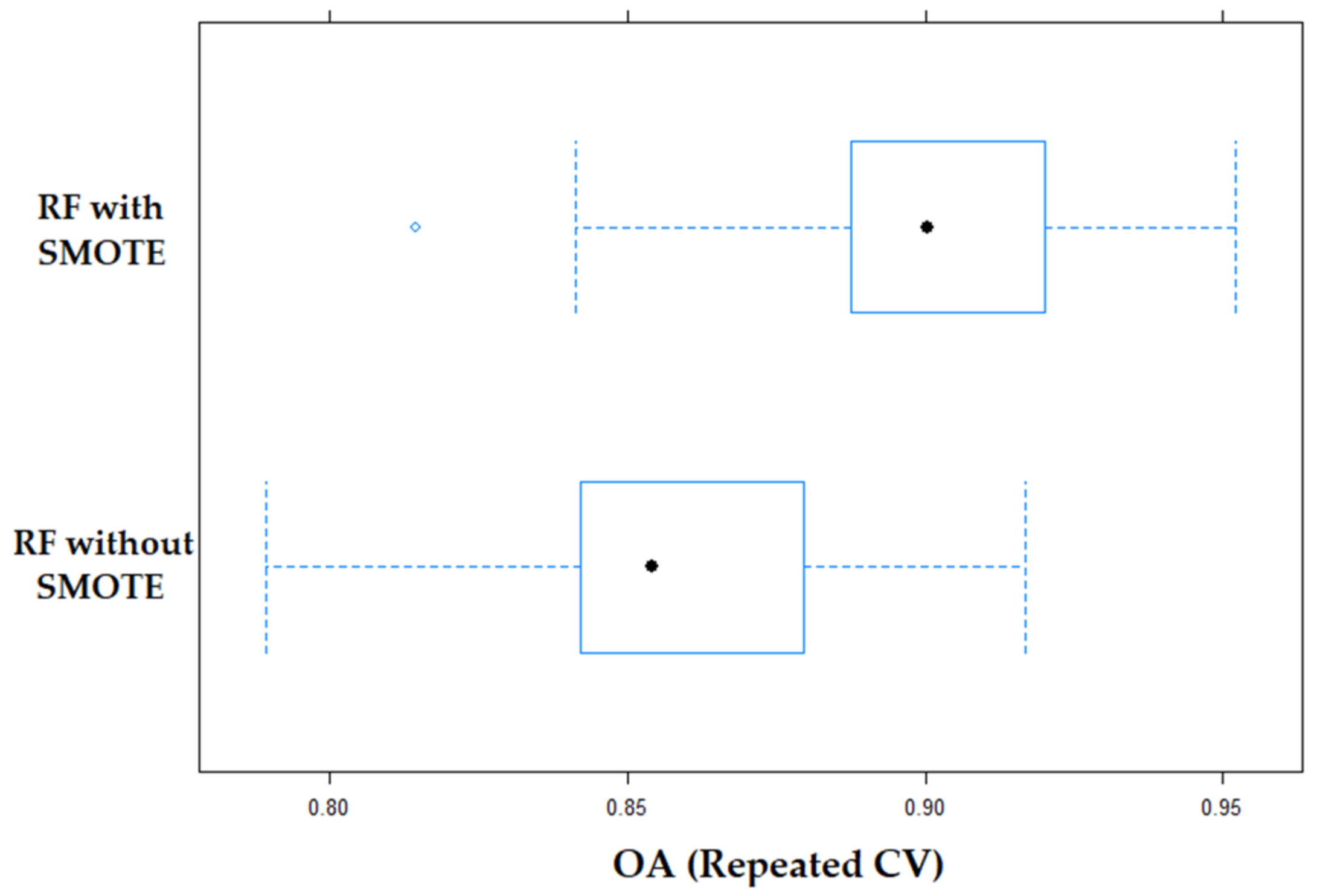
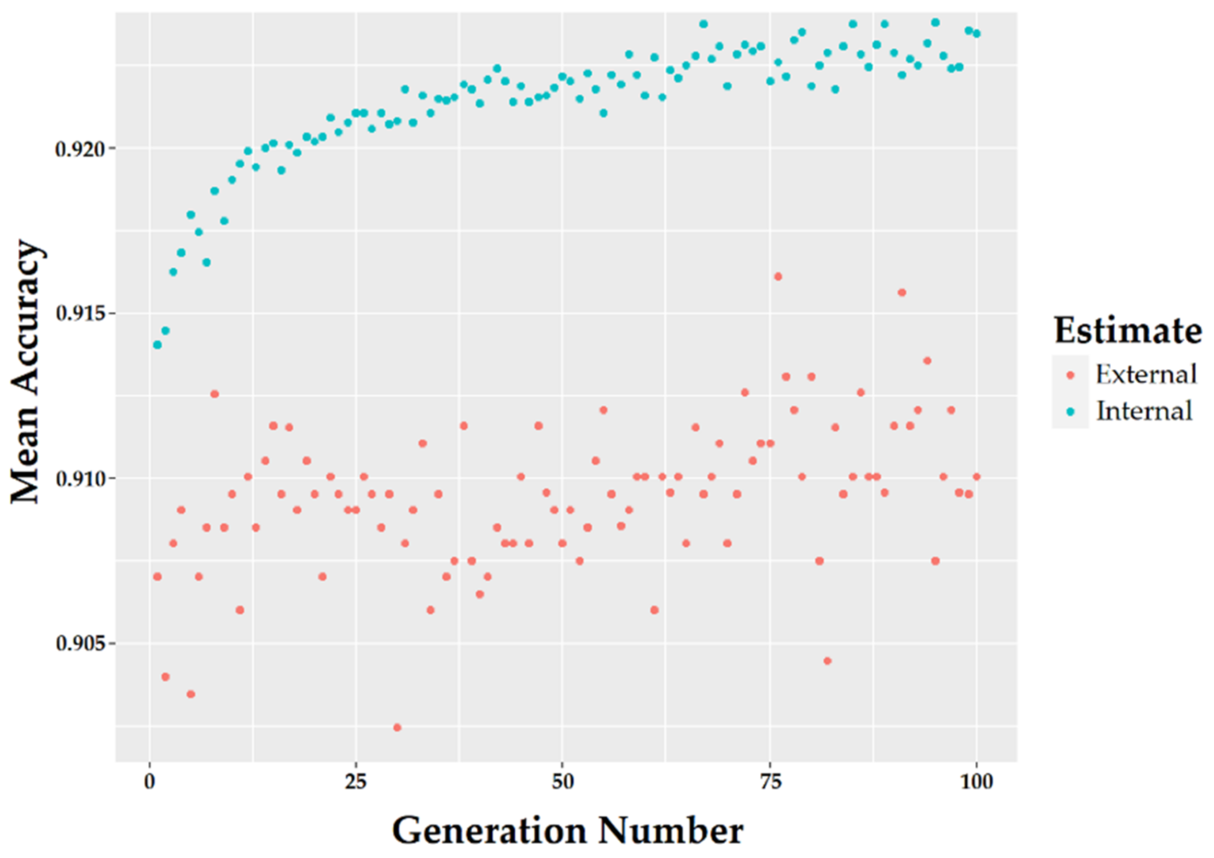
4.1. Data Balancing and Feature Selection Results
4.2. Optimal Hyperparameters Tuning
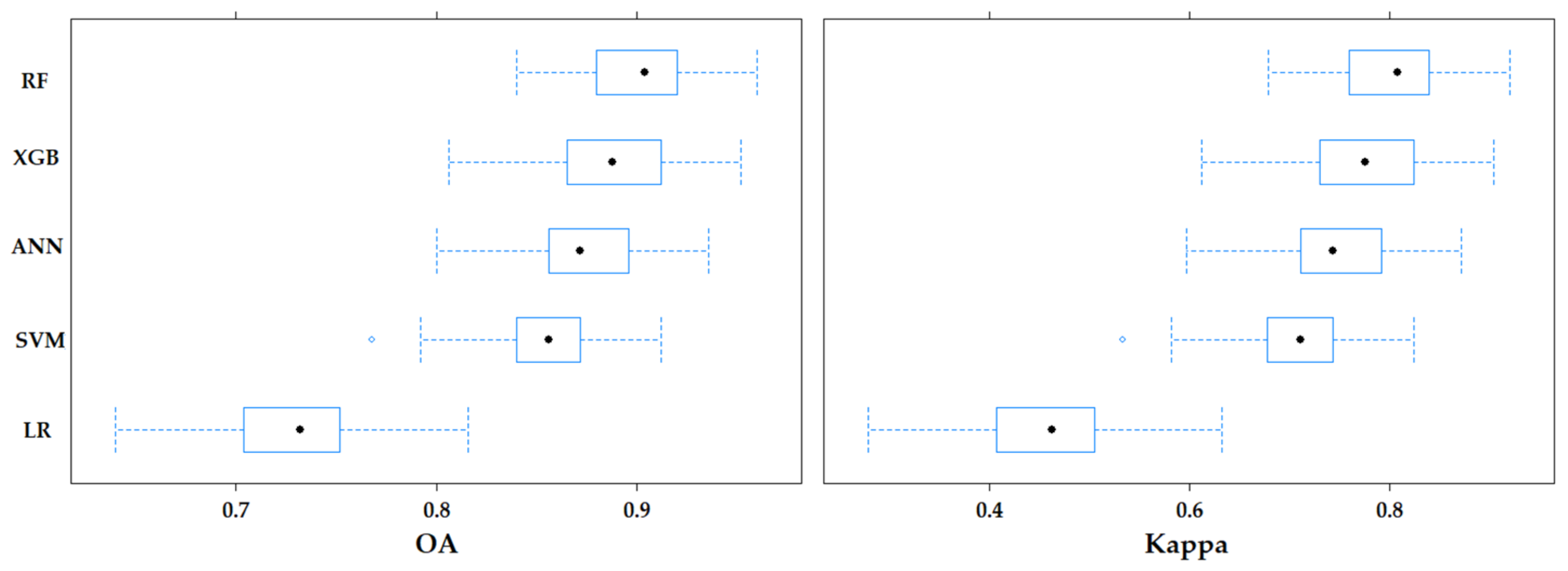
4.3. Machine Learning Method Selection
4.4. Classification Results
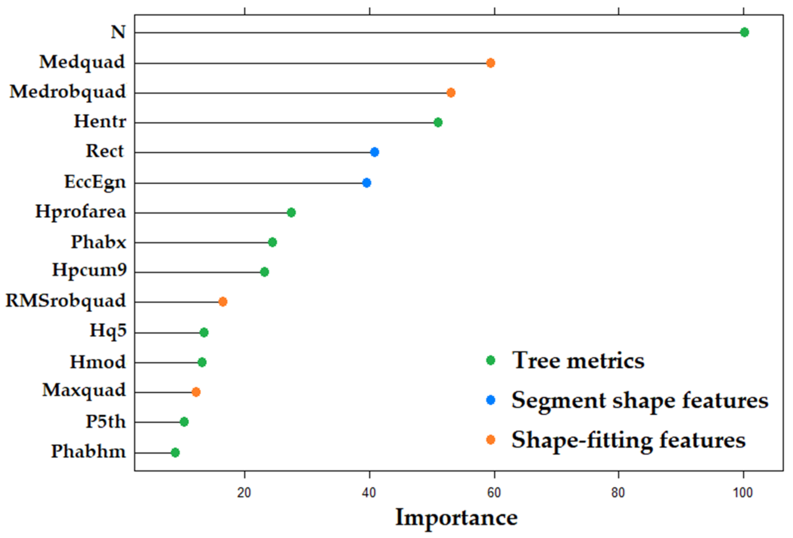
4.5. Variable Importance
5. Discussion
5.1. The ITD Strategy and the Resulting Accuracy Improvements
5.2. Machine Learning Method Selection
5.3. Classification Results
Classification Results Depending on the Forest Type
5.4. Variable Importance
6. Conclusions
Author Contributions
Funding
Data Availability Statement
Acknowledgments
Conflicts of Interest
References
- Wulder, M.A.; Coops, N.C.; Hudak, A.T.; Morsdorf, F.; Nelson, R.; Newnham, G.; Vastaranta, M. Status and Prospects for LiDAR Remote Sensing of Forested Ecosystems. Can. J. Remote Sens. 2013, 39, 37–41. [Google Scholar] [CrossRef] [Green Version]
- Hyyppä, J.; Inkinen, M. Detecting and Estimating Attributes for Single Trees Using Laser Scanner. Photogramm. J. Finl. 1999, 16, 27–42. [Google Scholar]
- Zhen, Z.; Quackenbush, L.J.; Zhang, L. Trends in Automatic Individual Tree Crown Detection and Delineation—Evolution of LiDAR Data. Remote Sens. 2016, 8, 333. [Google Scholar] [CrossRef] [Green Version]
- Hyyppä, J.; Schardt, M.; Haggrén, H.; Koch, B.; Lohr, U.; Paananen, R.; Scherrer, H.; Luukkonen, H.; Ziegler, M.; Hyyppä, H.; et al. HIGH-SCAN: The First European-Wide Attempt to Derive Single-Tree Information from Laserscanner Data. Photogramm. J. Finl. 2001, 17, 58–68. [Google Scholar]
- Koch, B.; Heyder, U.; Weinacker, H. Detection of Individual Tree Crowns in Airborne Lidar Data. Photogramm. Eng. Remote Sens. 2006, 72, 357–363. [Google Scholar] [CrossRef] [Green Version]
- Popescu, S.C.; Wynne, R.H.; Nelson, R.F. Estimating Plot-Level Tree Heights with Lidar: Local Filtering with a Canopy-Height Based Variable Window Size. Comput. Electron. Agric. 2002, 37, 71–95. [Google Scholar] [CrossRef]
- Ferraz, A.; Saatchi, S.; Mallet, C.; Meyer, V. Lidar Detection of Individual Tree Size in Tropical Forests. Remote Sens. Environ. 2016, 183, 318–333. [Google Scholar] [CrossRef]
- Silva, C.A.; Hudak, A.T.; Vierling, L.A.; Loudermilk, E.L.; O’Brien, J.J.; Hiers, J.K.; Jack, S.B.; Gonzalez-Benecke, C.; Lee, H.; Falkowski, M.J.; et al. Imputation of Individual Longleaf Pine (Pinus palustris Mill.) Tree Attributes from Field and LiDAR Data. Can. J. Remote Sens. 2016, 42, 554–573. [Google Scholar] [CrossRef]
- Persson, A.; Holmgren, J.; Soderman, U. Detecting and Measuring Individual Trees Using an Airborne Laser Scanner. Photogramm. Eng. Remote Sens. 2002, 68, 925–932. [Google Scholar]
- Hamraz, H.; Contreras, M.A.; Zhang, J. A Robust Approach for Tree Segmentation in Deciduous Forests Using Small-Footprint Airborne LiDAR Data. Int. J. Appl. Earth Obs. Geoinf. 2016, 52, 532–541. [Google Scholar] [CrossRef] [Green Version]
- Wu, B.; Yu, B.; Wu, Q.; Huang, Y.; Chen, Z.; Wu, J. Individual Tree Crown Delineation Using Localized Contour Tree Method and Airborne LiDAR Data in Coniferous Forests. Int. J. Appl. Earth Obs. Geoinf. 2016, 52, 82–94. [Google Scholar] [CrossRef]
- Wang, X.-H.; Zhang, Y.-Z.; Xu, M.-M. A Multi-Threshold Segmentation for Tree-Level Parameter Extraction in a Deciduous Forest Using Small-Footprint Airborne LiDAR Data. Remote Sens. 2019, 11, 2109. [Google Scholar] [CrossRef] [Green Version]
- Stereńczak, K.; Kraszewski, B.; Mielcarek, M.; Piasecka, Ż.; Lisiewicz, M.; Heurich, M. Mapping Individual Trees with Airborne Laser Scanning Data in an European Lowland Forest Using a Self-Calibration Algorithm. Int. J. Appl. Earth Obs. Geoinf. 2020, 93, 102191. [Google Scholar] [CrossRef]
- Khosravipour, A.; Skidmore, A.K.; Wang, T.; Isenburg, M.; Khoshelham, K. Effect of Slope on Treetop Detection Using a LiDAR Canopy Height Model. ISPRS J. Photogramm. Remote Sens. 2015, 104, 44–52. [Google Scholar] [CrossRef]
- Keränen, J.; Maltamo, M.; Packalen, P. Effect of Flying Altitude, Scanning Angle and Scanning Mode on the Accuracy of ALS Based Forest Inventory. Int. J. Appl. Earth Obs. Geoinf. 2016, 52, 349–360. [Google Scholar] [CrossRef]
- Liu, J.; Skidmore, A.K.; Jones, S.; Wang, T.; Heurich, M.; Zhu, X.; Shi, Y. Large Off-Nadir Scan Angle of Airborne LiDAR Can Severely Affect the Estimates of Forest Structure Metrics. ISPRS J. Photogramm. Remote Sens. 2018, 136, 13–25. [Google Scholar] [CrossRef]
- Khosravipour, A.; Skidmore, A.K.; Isenburg, M.; Wang, T.; Hussin, Y.A. Generating Pit-Free Canopy Height Models from Airborne Lidar. Photogramm. Eng. Remote Sens. 2014, 80, 863–872. [Google Scholar] [CrossRef]
- Chen, Q.; Baldocchi, D.; Gong, P.; Kelly, M. Isolating Individual Trees in a Savanna Woodland Using Small Footprint Lidar Data. Photogramm. Eng. Remote Sens. 2006, 72, 923–932. [Google Scholar] [CrossRef] [Green Version]
- Lee, H.; Slatton, K.C.; Roth, B.E.; Cropper, W.P. Adaptive Clustering of Airborne LiDAR Data to Segment Individual Tree Crowns in Managed Pine Forests. Int. J. Remote Sens. 2010, 31, 117–139. [Google Scholar] [CrossRef]
- Li, W.; Guo, Q.; Jakubowski, M.K.; Kelly, M. A New Method for Segmenting Individual Trees from the Lidar Point Cloud. Photogramm. Eng. Remote Sens. 2012, 78, 75–84. [Google Scholar] [CrossRef] [Green Version]
- Heinzel, J.N.; Weinacker, H.; Koch, B. Prior-Knowledge-Based Single-Tree Extraction. Int. J. Remote Sens. 2011, 32, 4999–5020. [Google Scholar] [CrossRef]
- Ene, L.; Næsset, E.; Gobakken, T. Single Tree Detection in Heterogeneous Boreal Forests Using Airborne Laser Scanning and Area-Based Stem Number Estimates. Int. J. Remote Sens. 2012, 33, 5171–5193. [Google Scholar] [CrossRef]
- Reitberger, J.; Schnörr, C.; Krzystek, P.; Stilla, U. 3D Segmentation of Single Trees Exploiting Full Waveform LIDAR Data. ISPRS J. Photogramm. Remote Sens. 2009, 64, 561–574. [Google Scholar] [CrossRef]
- Gupta, S.; Weinacker, H.; Koch, B. Comparative Analysis of Clustering-Based Approaches for 3-D Single Tree Detection Using Airborne Fullwave Lidar Data. Remote Sens. 2010, 2, 968–989. [Google Scholar] [CrossRef] [Green Version]
- Dong, T.; Zhou, Q.; Gao, S.; Shen, Y. Automatic Detection of Single Trees in Airborne Laser Scanning Data through Gradient Orientation Clustering. Forests 2018, 9, 291. [Google Scholar] [CrossRef] [Green Version]
- Zhao, D.; Pang, Y.; Li, Z.; Sun, G. Filling Invalid Values in a Lidar-Derived Canopy Height Model with Morphological Crown Control. Int. J. Remote Sens. 2013, 34, 4636–4654. [Google Scholar] [CrossRef]
- Lisiewicz, M.; Kamińska, A.; Stereńczak, K. Recognition of Specified Errors of Individual Tree Detection Methods Based on Canopy Height Model. Remote Sens. Appl. Soc. Environ. 2022, 25, 100690. [Google Scholar] [CrossRef]
- Lindberg, E.; Eysn, L.; Hollaus, M.; Holmgren, J.; Pfeifer, N. Delineation of Tree Crowns and Tree Species Classification From Full-Waveform Airborne Laser Scanning Data Using 3-D Ellipsoidal Clustering. IEEE J. Sel. Top. Appl. Earth Obs. Remote Sens. 2014, 7, 3174–3181. [Google Scholar] [CrossRef] [Green Version]
- Liu, T.; Im, J.; Quackenbush, L.J. A Novel Transferable Individual Tree Crown Delineation Model Based on Fishing Net Dragging and Boundary Classification. ISPRS J. Photogramm. Remote Sens. 2015, 110, 34–47. [Google Scholar] [CrossRef]
- Dai, W.; Yang, B.; Dong, Z.; Shaker, A. A New Method for 3D Individual Tree Extraction Using Multispectral Airborne LiDAR Point Clouds. ISPRS J. Photogramm. Remote Sens. 2018, 144, 400–411. [Google Scholar] [CrossRef]
- Jing, L.; Hu, B.; Li, J.; Noland, T. Automated Delineation of Individual Tree Crowns from Lidar Data by Multi-Scale Analysis and Segmentation. Photogramm. Eng. Remote Sens. 2012, 78, 1275–1284. [Google Scholar] [CrossRef]
- Wolf (né Straub), B.-M.; Heipke, C. Automatic Extraction and Delineation of Single Trees from Remote Sensing Data. Mach. Vis. Appl. 2007, 18, 317–330. [Google Scholar] [CrossRef]
- Polewski, P.; Yao, W.; Heurich, M.; Krzystek, P.; Stilla, U. Free Shape Context Descriptors Optimized with Genetic Algorithm for the Detection of Dead Tree Trunks in ALS Point Clouds. In Proceedings of the ISPRS Annals of the Photogrammetry, Remote Sensing and Spatial Information Sciences, ISPRS Geospatial Week 2015, La Grande Motte, France, 28 September–3 October 2015; Volume II-3-W5. pp. 41–48. [Google Scholar]
- West, K.F.; Webb, B.N.; Lersch, J.R.; Pothier, S.; Triscari, J.M.; Iverson, A.E. Context-Driven Automated Target Detection in 3D Data. In Proceedings of the Automatic Target Recognition XIV, Bellingham, WA, USA, 21 September 2004; SPIE: Bellingham, WA, USA, 2004; Volume 5426, pp. 133–143. [Google Scholar]
- Chehata, N.; Guo, L.; Mallet, C. Airborne Lidar Feature Selection for Urban Classification Using Random Forests. In Proceedings of the Laserscanning, Paris, France, 1–2 September 2009. [Google Scholar]
- Weinmann, M.; Jutzi, B.; Mallet, C. Semantic 3D Scene Interpretation: A Framework Combining Optimal Neighborhood Size Selection with Relevant Features. ISPRS Ann. Photogramm. Remote Sens. Spat. Inf. Sci. 2014, II-3, 181–188. [Google Scholar] [CrossRef]
- Kathuria, A.; Turner, R.; Stone, C.; Duque-Lazo, J.; West, R. Development of an Automated Individual Tree Detection Model Using Point Cloud LiDAR Data for Accurate Tree Counts in a Pinus Radiata Plantation. Aust. For. 2016, 79, 126–136. [Google Scholar] [CrossRef]
- Wan Mohd Jaafar, W.S.; Woodhouse, I.H.; Silva, C.A.; Omar, H.; Abdul Maulud, K.N.; Hudak, A.T.; Klauberg, C.; Cardil, A.; Mohan, M. Improving Individual Tree Crown Delineation and Attributes Estimation of Tropical Forests Using Airborne LiDAR Data. Forests 2018, 9, 759. [Google Scholar] [CrossRef] [Green Version]
- Holmgren, J.; Lindberg, E. Tree Crown Segmentation Based on a Tree Crown Density Model Derived from Airborne Laser Scanning. Remote Sens. Lett. 2019, 10, 1143–1152. [Google Scholar] [CrossRef]
- Mongus, D.; Žalik, B. An Efficient Approach to 3D Single Tree-Crown Delineation in LiDAR Data. ISPRS J. Photogramm. Remote Sens. 2015, 108, 219–233. [Google Scholar] [CrossRef]
- Krzystek, P.; Serebryanyk, A.; Schnörr, C.; Červenka, J.; Heurich, M. Large-Scale Mapping of Tree Species and Dead Trees in Šumava National Park and Bavarian Forest National Park Using Lidar and Multispectral Imagery. Remote Sens. 2020, 12, 661. [Google Scholar] [CrossRef] [Green Version]
- Lisiewicz, M.; Kamińska, A.; Kraszewski, B.; Stereńczak, K. Correcting the Results of CHM-Based Individual Tree Detection Algorithms to Improve Their Accuracy and Reliability. Remote Sens. 2022, 14, 1822. [Google Scholar] [CrossRef]
- Axelsson, P. DEM Generation from Laser Scanner Data Using Adaptive TIN Models. Int. Arch. Photogramm. Remote Sens. 2000, 33, 110–117. [Google Scholar]
- Popescu, S.C.; Wynne, R.H. Seeing the Trees in the Forest. Photogramm. Eng. Remote Sens. 2004, 70, 589–604. [Google Scholar] [CrossRef] [Green Version]
- Roussel, J.-R.; Auty, D.; Coops, N.C.; Tompalski, P.; Goodbody, T.R.H.; Meador, A.S.; Bourdon, J.-F.; de Boissieu, F.; Achim, A. LidR: An R Package for Analysis of Airborne Laser Scanning (ALS) Data. Remote Sens. Environ. 2020, 251, 112061. [Google Scholar] [CrossRef]
- Roussel, J.-R.; Auty, D.; De Boissieu, F.; Meador, A.S.; Bourdon, J.-F.; Demetrios, G.; Steinmeier, L.; Adaszewski, S. lidR: Airborne LiDAR Data Manipulation and Visualization for Forestry Applications; Version 4.0.1; R Core Team: Vienna, Austria, 2022. [Google Scholar]
- R Core Team R. A language and environment for statistical computing; R Foundation for Statistical, Computing: Vienna, Austria, 2022; Available online: https://www.R-project.org/ (accessed on 21 June 2022).
- Silva, C.A.; Crookston, N.L.; Hudak, A.T.; Vierling, L.A.; Klauberg, C.; Cardil, A.; Hamamura, C. rLiDAR: LiDAR Data Processing and Visualization; Version 0.1.5; R Core Team: Vienna, Austria, 2022. [Google Scholar]
- McGaughey, R.J. FUSION/LDV: Software for LIDAR Data Analysis and Visualization; Version 4.40; US Department of Agriculture, Forest Service, Pacific Northwest Research Station, University of Washington: Seattle, WA, USA, 2022.
- Shannon, C.E. A Mathematical Theory of Communication. Bell Syst. Tech. J. 1948, 27, 379–423. [Google Scholar] [CrossRef] [Green Version]
- Woods, M.; Lim, K.; Treitz, P. Predicting Forest Stand Variables from LiDAR Data in the Great Lakes—St. Lawrence Forest of Ontario. For. Chron. 2008, 84, 827–839. [Google Scholar] [CrossRef]
- Detsch, F.; Meyer, H.; Möller, F.; Nauss, T.; Opgenoorth, L.; Reudenbach, C.; Environmental Informatics Marburg. uavRst: Unmanned Aerial Vehicle Remote Sensing Tools; Version 0.5.5. Available online: https://mran.microsoft.com/snapshot/2019-02-21/web/packages/uavRst/index.html (accessed on 21 June 2022).
- Rosin, P.L. Computing Global Shape Measures. In Handbook of Pattern Recognition and Computer Vision; World Scientific: Singapore, 2005; pp. 177–196. ISBN 978-981-256-105-3. [Google Scholar]
- Haralick, R.M. A Measure for Circularity of Digital Figures. IEEE Trans. Syst. Man Cybern. 1974, SMC-4, 394–396. [Google Scholar] [CrossRef]
- Lucas, C.; Bouten, W.; Koma, Z.; Kissling, W.D.; Seijmonsbergen, A.C. Identification of Linear Vegetation Elements in a Rural Landscape Using LiDAR Point Clouds. Remote Sens. 2019, 11, 292. [Google Scholar] [CrossRef] [Green Version]
- Hoppe, H.; DeRose, T.; Duchamp, T.; McDonald, J.; Stuetzle, W. Surface Reconstruction from Unorganized Points. SIGGRAPH Comput. Graph. 1992, 26, 71–78. [Google Scholar] [CrossRef]
- Pfeifer, N.; Mandlburger, G.; Otepka, J.; Karel, W. OPALS—A Framework for Airborne Laser Scanning Data Analysis. Comput. Environ. Urban Syst. 2014, 45, 125–136. [Google Scholar] [CrossRef]
- Mandlburger, G.; Otepka, J.; Karel, W.; Wagner, W.; Pfeifer, N. Orientation and Processing of Airborne Laser Scanning Data (OPALS)—Concept and First Results of a Comprehensive ALS Software. In Proceedings of the Laser Scanning 2009, IAPRS, Paris, France, 1–2 September 2009; Volume XXXVIII. Part 3/W8. [Google Scholar]
- He, H.; Bai, Y.; Garcia, E.A.; Li, S. ADASYN: Adaptive Synthetic Sampling Approach for Imbalanced Learning. In Proceedings of the 2008 IEEE International Joint Conference on Neural Networks (IEEE World Congress on Computational Intelligence), Hong Kong, China, 1–8 June 2008; pp. 1322–1328. [Google Scholar]
- Mitchell, M. An Introduction to Genetic Algorithms; Complex Adaptive Systems; A Bradford Book: Cambridge, MA, USA, 1996; ISBN 978-0-262-13316-6. [Google Scholar]
- Breiman, L. Random Forests. Mach. Learn. 2001, 45, 5–32. [Google Scholar] [CrossRef] [Green Version]
- Geurts, P.; Ernst, D.; Wehenkel, L. Extremely Randomized Trees. Mach. Learn 2006, 63, 3–42. [Google Scholar] [CrossRef] [Green Version]
- Chen, T.; Guestrin, C. XGBoost: A Scalable Tree Boosting System. In Proceedings of the 22nd ACM SIGKDD International Conference on Knowledge Discovery and Data Mining, San Francisco, CA, USA, 13 August 2016; Association for Computing Machinery: New York, NY, USA, 2016; pp. 785–794. [Google Scholar]
- Ripley, B.D. Pattern Recognition and Neural Networks; Cambridge University Press: Cambridge, UK, 1996; ISBN 978-0-521-71770-0. [Google Scholar]
- Schmidhuber, J. Deep Learning in Neural Networks: An Overview. Neural Netw. 2015, 61, 85–117. [Google Scholar] [CrossRef] [Green Version]
- Cortes, C.; Vapnik, V. Support-Vector Networks. Mach. Learn. 1995, 20, 273–297. [Google Scholar] [CrossRef]
- Kebede, T.A.; Hailu, B.T.; Suryabhagavan, K.V. Evaluation of Spectral Built-up Indices for Impervious Surface Extraction Using Sentinel-2A MSI Imageries: A Case of Addis Ababa City, Ethiopia. Environ. Chall. 2022, 8, 100568. [Google Scholar] [CrossRef]
- Gašparović, M.; Dobrinić, D. Green Infrastructure Mapping in Urban Areas Using Sentinel-1 Imagery. Croat. J. For. Eng. (Online) 2021, 42, 337–356. [Google Scholar] [CrossRef]
- Cox, D.R. The Regression Analysis of Binary Sequences. J. R. Stat. Society. Ser. B (Methodol.) 1958, 20, 215–242. [Google Scholar] [CrossRef]
- Nelder, J.A.; Wedderburn, R.W.M. Generalized Linear Models. J. R. Stat. Society. Ser. A (Gen.) 1972, 135, 370–384. [Google Scholar] [CrossRef]
- Story, M. Accuracy Assessment: A User’s Perspective. Photogramm. Eng. Remote Sens. 1986, 52, 397–399. [Google Scholar]
- CRAN—Package Smotefamily. Available online: https://cran.r-project.org/web/packages/smotefamily/index.html (accessed on 19 July 2022).
- Kuhn, M. Building Predictive Models in R Using the Caret Package. J. Stat. Softw. 2008, 28, 1–26. [Google Scholar] [CrossRef] [Green Version]
- Scrucca, L. GA: A Package for Genetic Algorithms in R. J. Stat. Softw. 2013, 53, 1–37. [Google Scholar] [CrossRef] [Green Version]
- Wright, M.N.; Ziegler, A. Ranger: A Fast Implementation of Random Forests for High Dimensional Data in C++ and R. J. Stat. Softw. 2017, 77, 1–17. [Google Scholar] [CrossRef] [Green Version]
- Chen, T.; He, T.; Benesty, M.; Khotilovich, V.; Tang, Y.; Cho, H.; Chen, K.; Mitchell, R.; Cano, I.; Zhou, T.; et al. xgboost: Extreme Gradient Boosting; Version 1.6.0.1; R Core Team: Vienna, Austria, 2022. [Google Scholar]
- Karatzoglou, A.; Smola, A.; Hornik, K.; Zeileis, A. kernlab—An S4 Package for Kernel Methods in R. J. Stat. Softw. 2004, 11, 1–20. [Google Scholar] [CrossRef] [Green Version]
- Karatzoglou, A.; Smola, A.; Hornik, K.; Australia (NICTA); Maniscalco, M.; Teo, C.H. kernlab: Kernel-Based Machine Learning Lab; Version 0.9.29; R Core Team: Vienna, Austria, 2022. [Google Scholar]
- Venables, W.; Ripley, B. Modern Applied Statistics with S, 4th ed.; Springer: New York, NY, USA, 2002. [Google Scholar] [CrossRef]
- Kuhn, M.; Wing, J.; Weston, S.; Williams, A.; Keefer, C.; Engelhardt, A.; Cooper, T.; Mayer, Z.; Kenkel, B.; R Core Team; et al. caret: Classification and Regression Training; Version 6.0.92; R Core Team: Vienna, Austria, 2022. [Google Scholar]
- Pitkänen, J.; Maltamo, M.; Hyyppä, J.; Yu, X. Adaptive Methods for Individual Tree Detection on Airborne Laser Based Canopy Height Model. Int. Arch. Photogramm. Remote Sens. Spat. Inf. Sci. 2004, 36, 187–191. [Google Scholar]
- Yu, X.; Hyyppä, J.; Vastaranta, M.; Holopainen, M.; Viitala, R. Predicting Individual Tree Attributes from Airborne Laser Point Clouds Based on the Random Forests Technique. ISPRS J. Photogramm. Remote Sens. 2011, 66, 28–37. [Google Scholar] [CrossRef]
- Kaartinen, H.; Hyyppä, J.; Yu, X.; Vastaranta, M.; Hyyppä, H.; Kukko, A.; Holopainen, M.; Heipke, C.; Hirschmugl, M.; Morsdorf, F.; et al. An International Comparison of Individual Tree Detection and Extraction Using Airborne Laser Scanning. Remote Sens. 2012, 4, 950–974. [Google Scholar] [CrossRef] [Green Version]
- Kamińska, A.; Lisiewicz, M.; Stereńczak, K.; Kraszewski, B.; Sadkowski, R. Species-Related Single Dead Tree Detection Using Multi-Temporal ALS Data and CIR Imagery. Remote Sens. Environ. 2018, 219, 31–43. [Google Scholar] [CrossRef]
- Immitzer, M.; Atzberger, C.; Koukal, T. Tree Species Classification with Random Forest Using Very High Spatial Resolution 8-Band WorldView-2 Satellite Data. Remote Sens. 2012, 4, 2661–2693. [Google Scholar] [CrossRef] [Green Version]
- Corte, A.P.D.; Souza, D.V.; Rex, F.E.; Sanquetta, C.R.; Mohan, M.; Silva, C.A.; Zambrano, A.M.A.; Prata, G.; Alves de Almeida, D.R.; Trautenmüller, J.W.; et al. Forest Inventory with High-Density UAV-Lidar: Machine Learning Approaches for Predicting Individual Tree Attributes. Comput. Electron. Agric. 2020, 179, 105815. [Google Scholar] [CrossRef]
- Ballanti, L.; Blesius, L.; Hines, E.; Kruse, B. Tree Species Classification Using Hyperspectral Imagery: A Comparison of Two Classifiers. Remote Sens. 2016, 8, 445. [Google Scholar] [CrossRef] [Green Version]
- Dalponte, M.; Bruzzone, L.; Gianelle, D. Tree Species Classification in the Southern Alps Based on the Fusion of Very High Geometrical Resolution Multispectral/Hyperspectral Images and LiDAR Data. Remote Sens. Environ. 2012, 123, 258–270. [Google Scholar] [CrossRef]
- Harrell, F.E. Regression Modeling Strategies, 2nd ed.; Springer: New York, NY, USA, 2015. [Google Scholar] [CrossRef]
- Ahokas, E.; Kaasalainen, S.; Hyyppä, J.; Suomalainen, J. Calibration of the OPTECH ALTM 3100 Laser Scanner Intensity Data Using Brightness Targets. Int. Arch. Photogramm. Remote Sens. Spat. Inf. Sci. 2006, 36, 1–6. [Google Scholar]
- Kashani, A.G.; Olsen, M.J.; Parrish, C.E.; Wilson, N. A Review of LIDAR Radiometric Processing: From Ad Hoc Intensity Correction to Rigorous Radiometric Calibration. Sensors 2015, 15, 28099–28128. [Google Scholar] [CrossRef] [Green Version]
- Eysn, L.; Hollaus, M.; Lindberg, E.; Berger, F.; Monnet, J.-M.; Dalponte, M.; Kobal, M.; Pellegrini, M.; Lingua, E.; Mongus, D.; et al. A Benchmark of Lidar-Based Single Tree Detection Methods Using Heterogeneous Forest Data from the Alpine Space. Forests 2015, 6, 1721–1747. [Google Scholar] [CrossRef]


| Tree Metrics | Description | Software |
|---|---|---|
| N | number of points in each tree segment | lidr |
| Area | approximate actual area of a raster | |
| Phabhm | percentage of returns above mean height | |
| Hentr | entropy of height distribution—the normalized Shannon vertical complexity index [50] | |
| Phabx | percentage of returns above x | |
| Hpcum (x = 1,…,9) range = 1 | cumulative percentage of return in the ith layer, according to Woods et al. [51] | |
| P (x = 1,2,3,4,5) th | percentage of xth return | |
| Hmin | minimum height | rLidar |
| Hmax | maximum height | |
| Hmean | mean height | |
| Hmed | median height | |
| Hmod | height mode | |
| Hsd | standard deviation of height distribution | |
| Hvar | height variance | |
| Hcv | coefficient of variation of height | |
| Hskew | skewness of height distribution | |
| Hkurt | kurtosis of height distribution | |
| Hq (x = 1,5,…,95,99) range = 5 | xth percentile (quantile) of height distribution | |
| Ewidth | tree crown width in eastern direction | |
| Nwidth | tree crown width in northern direction | |
| Diq | interquartile distance | FUSION |
| Haad | Average Absolute Deviation of height | |
| Hmadmed | median of the absolute deviations from the overall median | |
| Hmadmod | median of the absolute deviations from the overall mode | |
| HL (x = 1,2,3,4) | L-moments (λ1, λ2, λ3, λ4) | |
| HLcv | L-moments coefficient of variation τ2 = λ1/λ2 | |
| HLskew | L-moments skewness τ2 = λ3/λ2 | |
| HLkurt | = λ4/λ2 | |
| Hcrr | canopy relief ratio ((Hmean − Hmin)/(Hmax − Hmin)) | |
| Hsqmsq | generalized means for the 2nd power (height quadratic mean) | |
| Hsqmcube | generalized means for the 3rd power (height cubic mean) | |
| Hprofarea | area under the height percentile profile or curve |
| Segment Shape Features | Description |
| Lngt | length—largest dimension of a polygon |
| Elng | elongation—the ratio of the width and diameter of polygon |
| EccBB | eccentricity-bounding box—ratio of the width and diameter of bounding box of polygon |
| Solid | solidity—the ratio of polygon area and area of the convex hull |
| EccEgn | eigenvalue of eccentricity matrix |
| Rect | rectangularity—the ratio of the area of the segment to the area of its MBR |
| CircHar | Haralick’s circularity of a shape |
| Convex | convexity—the ratio of the eigenvalues (inertia axis) |
| Eigenvalue-Based Features | Description |
|---|---|
| EgnLrg | largest eigenvalue e1 |
| EgnMdm | medium eigenvalue e2 |
| EgnSml | smallest eigenvalue e3 |
| Lnr | linearity (e1 − e2)/e1 |
| Plnr | planarity (e2 − e3)/e1 |
| Sph | sphericity e3/e1 |
| Anstr | anisotropy (e1 − e3)/e1 |
| Curv | curvature e3/(e1 + e2 + e3) |
| Omnivar | omnivariance |
| Eigentr | Eigen entropy—(e1 ln(e1) + e2 ln(e2) + e3 ln(e3)) |
| Eigensum | sum of eigenvalues e1 + e2 + e3 |
| Shape-Fitting Features | Description |
|---|---|
| Minquad | minimum of residuals fitting points to polynomial surface |
| Maxquad | maximum of residuals fitting points to polynomial surface |
| Medquad | median of residuals fitting points to polynomial surface |
| RMSquad | RMS of residuals fitting points to polynomial surface |
| Minrobquad | robust minimum of residuals fitting points to polynomial surface |
| Maxrobquad | robust maximum of residuals fitting points to polynomial surface |
| Medrobquad | robust median of residuals fitting points to polynomial surface |
| RMSrobquad | robust RMS of residuals fitting points to polynomial surface |
| Algorithm | Optimal Hyperparameters | Method/R Package |
|---|---|---|
| RF | splitrule = extratrees ntree = 2000 min.node.size = 1 mtry = 4 num.random.splits = 3 | Extremely Randomized Trees/ranger [75] |
| XGB | nrounds = 1500 max_depth = 4 eta = 0.1 gamma = 0 | xgboost [76] |
| ANN | size = 36 decay = 0.2 | polynomial kernel/kernlab [77,78] |
| SVM | degree = 3 scale = 1 C = 0.1 | feed-forward with single hidden layer/nnet [79] |
| LR | family = binomial | glm/caret [80] |
| Classifier | OA [%] | κ |
|---|---|---|
| RF | 89.0 | 0.757 |
| XGB | 88.8 | 0.750 |
| ANN | 84.1 | 0.657 |
| SVM | 82.5 | 0.625 |
| LR | 74.1 | 0.431 |
| Plot Type | Pred/Ref | True | False | UA |
|---|---|---|---|---|
| Mixed (all 8 plots) | true | 257 | 15 | 94.5% |
| false | 32 | 124 | 79.5% | |
| PA | 88.9% | 89.2% | OA= 89.0%; κ = 0.757 |
| Plot Type | Pred/Ref | True | False | UA |
|---|---|---|---|---|
| Deciduous (5 plots) | true | 113 | 7 | 94.2% |
| false | 14 | 46 | 76.7% | |
| PA | 89.0% | 86.8% | OA = 88.3%; κ = 0.730 | |
| Coniferous (2 plots) | true | 118 | 6 | 95.2% |
| false | 17 | 71 | 80.7% | |
| PA | 87.4% | 92.2% | OA = 89.2%; κ = 0.772 | |
| Mixed (1 plot) | true | 26 | 2 | 92.9% |
| false | 1 | 7 | 87.5% | |
| PA | 96.3% | 77.8% | OA = 91.7%; κ = 0.769 |
Publisher’s Note: MDPI stays neutral with regard to jurisdictional claims in published maps and institutional affiliations. |
© 2022 by the authors. Licensee MDPI, Basel, Switzerland. This article is an open access article distributed under the terms and conditions of the Creative Commons Attribution (CC BY) license (https://creativecommons.org/licenses/by/4.0/).
Share and Cite
Brodić, N.; Cvijetinović, Ž.; Milenković, M.; Kovačević, J.; Stančić, N.; Mitrović, M.; Mihajlović, D. Refinement of Individual Tree Detection Results Obtained from Airborne Laser Scanning Data for a Mixed Natural Forest. Remote Sens. 2022, 14, 5345. https://doi.org/10.3390/rs14215345
Brodić N, Cvijetinović Ž, Milenković M, Kovačević J, Stančić N, Mitrović M, Mihajlović D. Refinement of Individual Tree Detection Results Obtained from Airborne Laser Scanning Data for a Mixed Natural Forest. Remote Sensing. 2022; 14(21):5345. https://doi.org/10.3390/rs14215345
Chicago/Turabian StyleBrodić, Nenad, Željko Cvijetinović, Milutin Milenković, Jovan Kovačević, Nikola Stančić, Momir Mitrović, and Dragan Mihajlović. 2022. "Refinement of Individual Tree Detection Results Obtained from Airborne Laser Scanning Data for a Mixed Natural Forest" Remote Sensing 14, no. 21: 5345. https://doi.org/10.3390/rs14215345