
RecepNet: Network with Large Receptive Field for Real-Time Semantic Segmentation and Application for Blue-Green Algae
 , , ,
, , ,  , , , , , and
Abstract
:1. Introduction
- We propose an effective stem block. It is used in both the detail path and semantic path for fast downsampling while expanding channels flexibly;
- Gather–expand–search (GES) layer, a lightweight downsampling network, is proposed for the semantic path to achieve fast and robust feature extraction. It obtains rich spatial and semantic information by gathering the semantic features, expanding to large dimensions, and searching for multi-resolution features;
- We design a detail stage pattern. It cleans the redundant information, reserves the high-resolution information in the spatial dimension, and improves feature representation;
- A novel training boosting strategy is devised. It improves accuracy by strengthening and recalibrating features in the training phases.
2. Literature Review
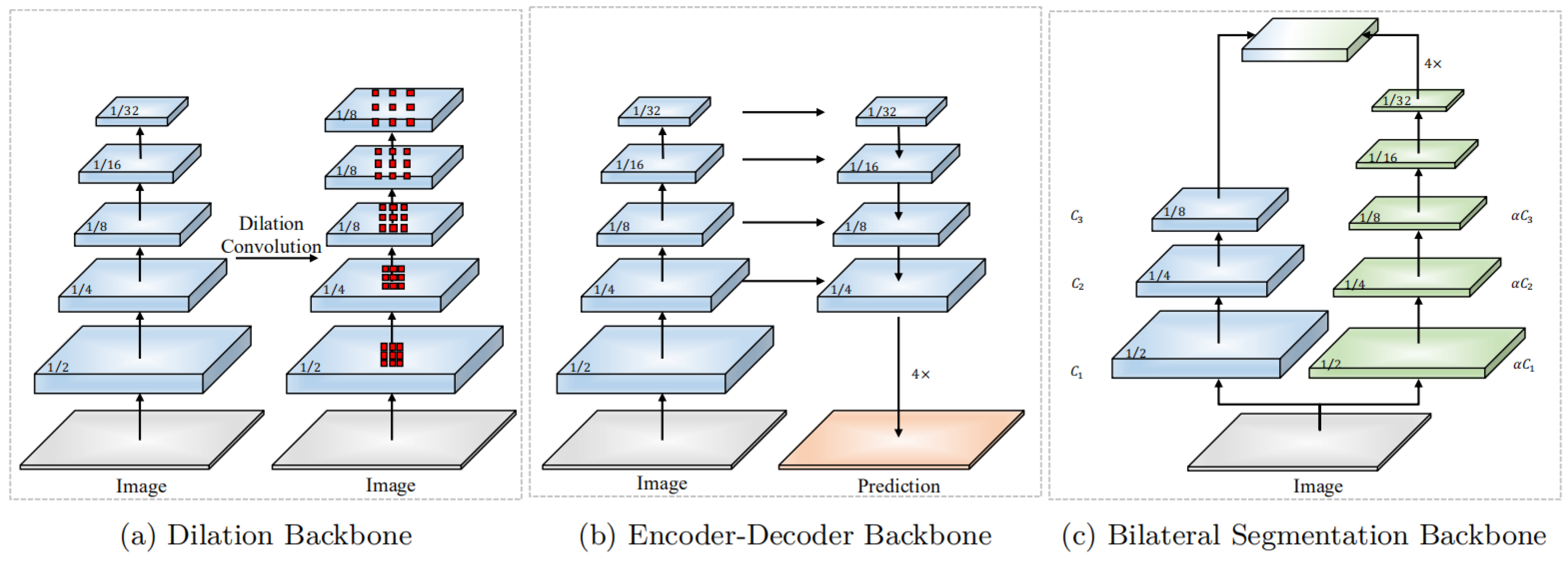
2.1. High-Performance Semantic Segmentation
2.2. Real-Time Semantic Segmentation
3. Methodology
3.1. Overview
3.1.1. Core Concept of RecepNet
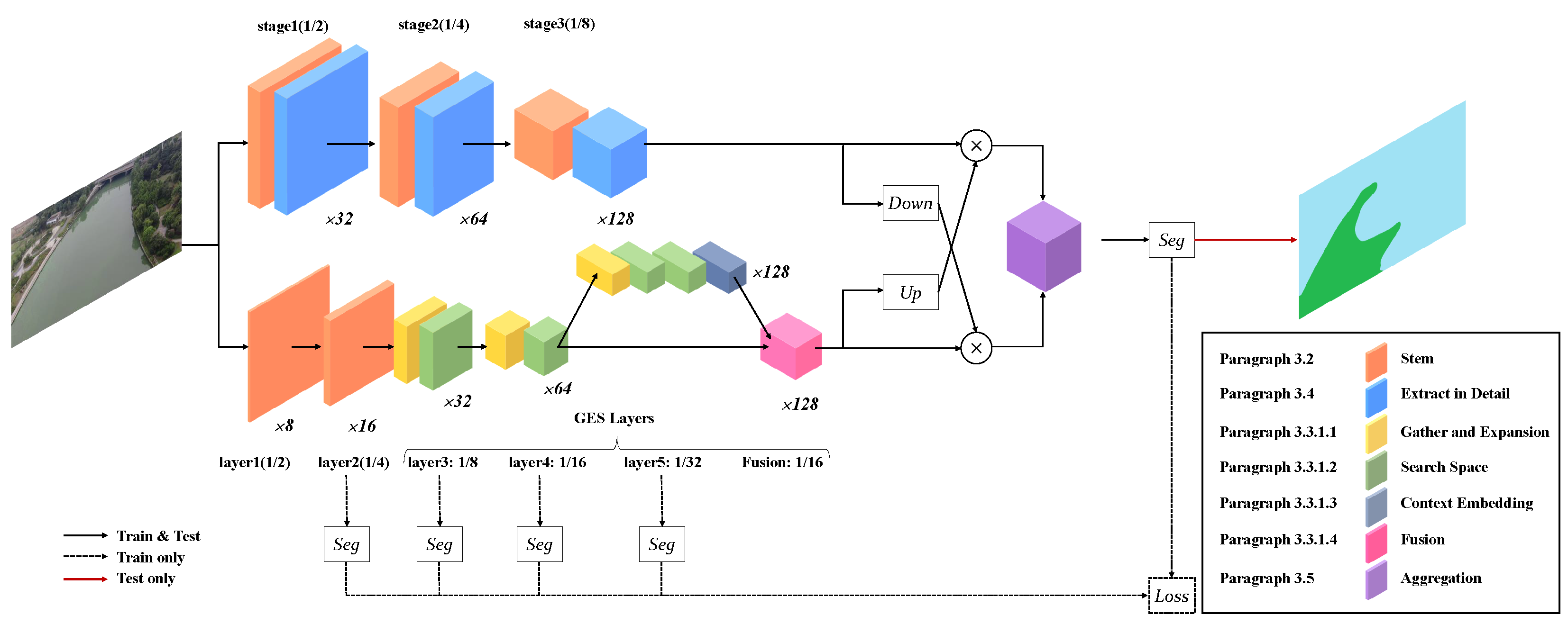
3.1.2. Overall Structure
3.1.3. Block Design
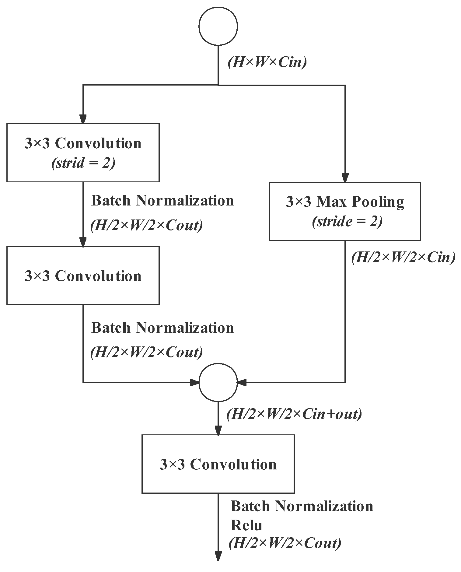
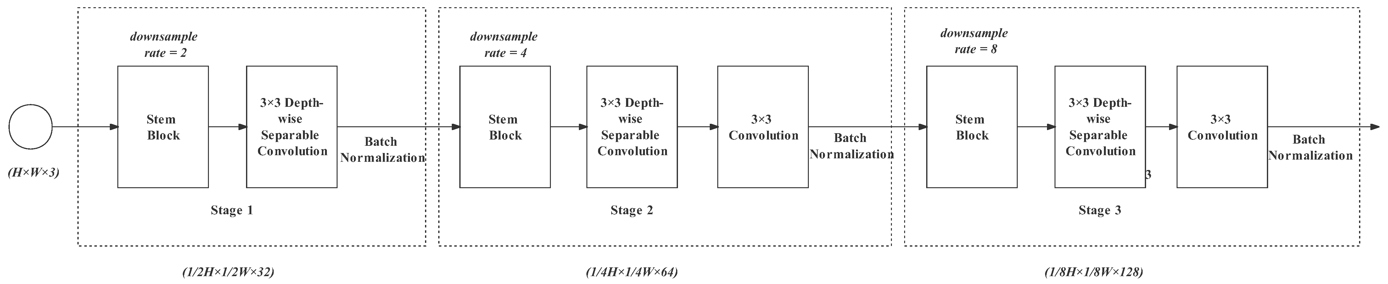
3.2. Stem Block
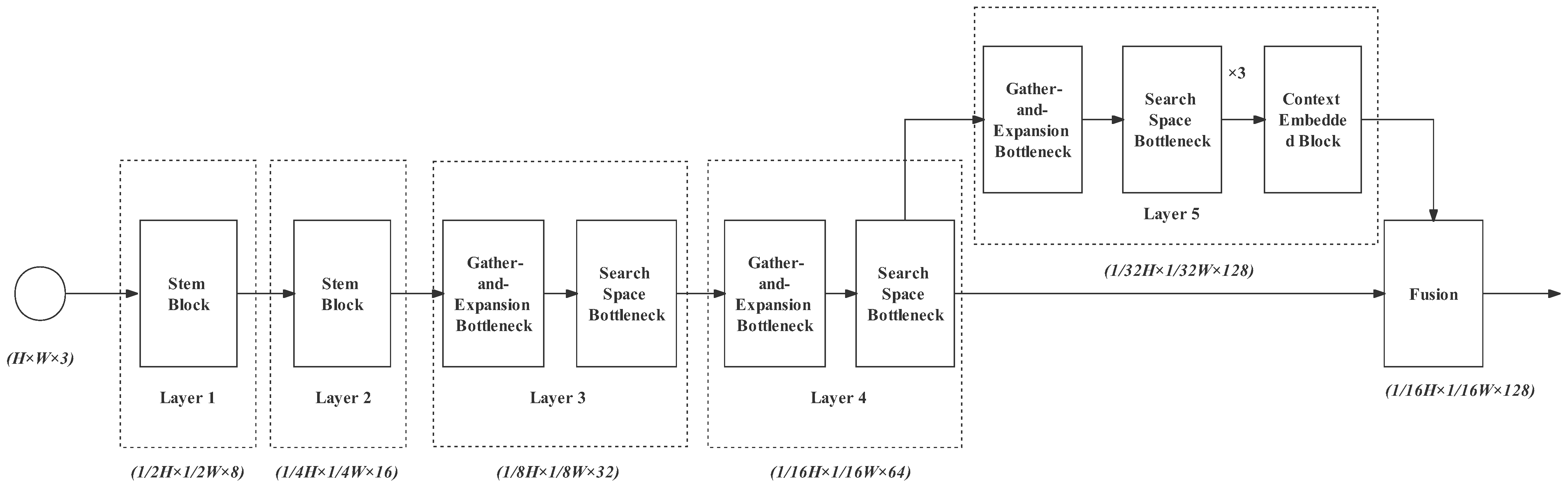
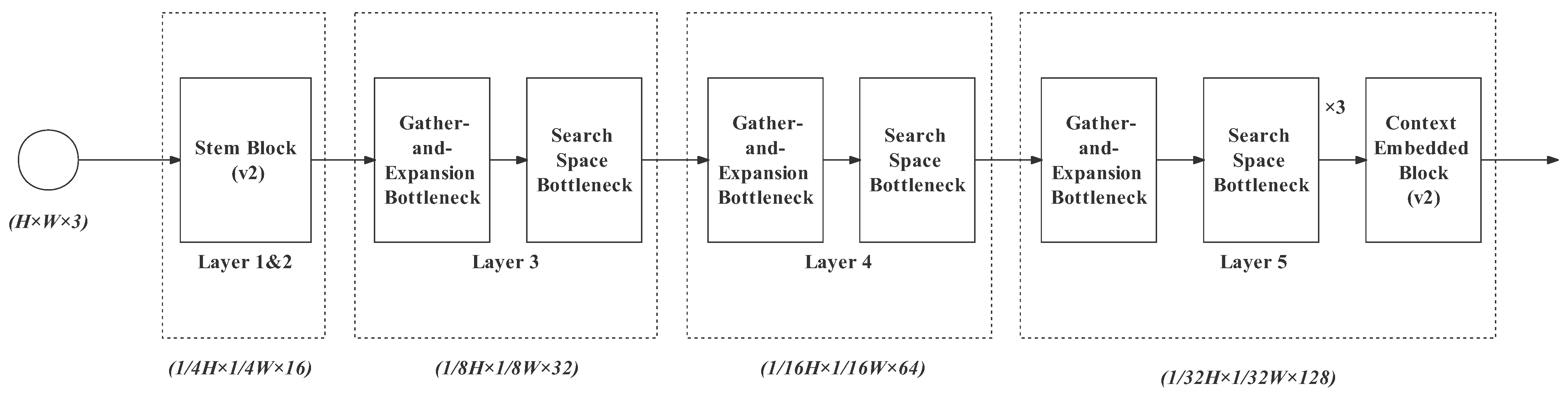
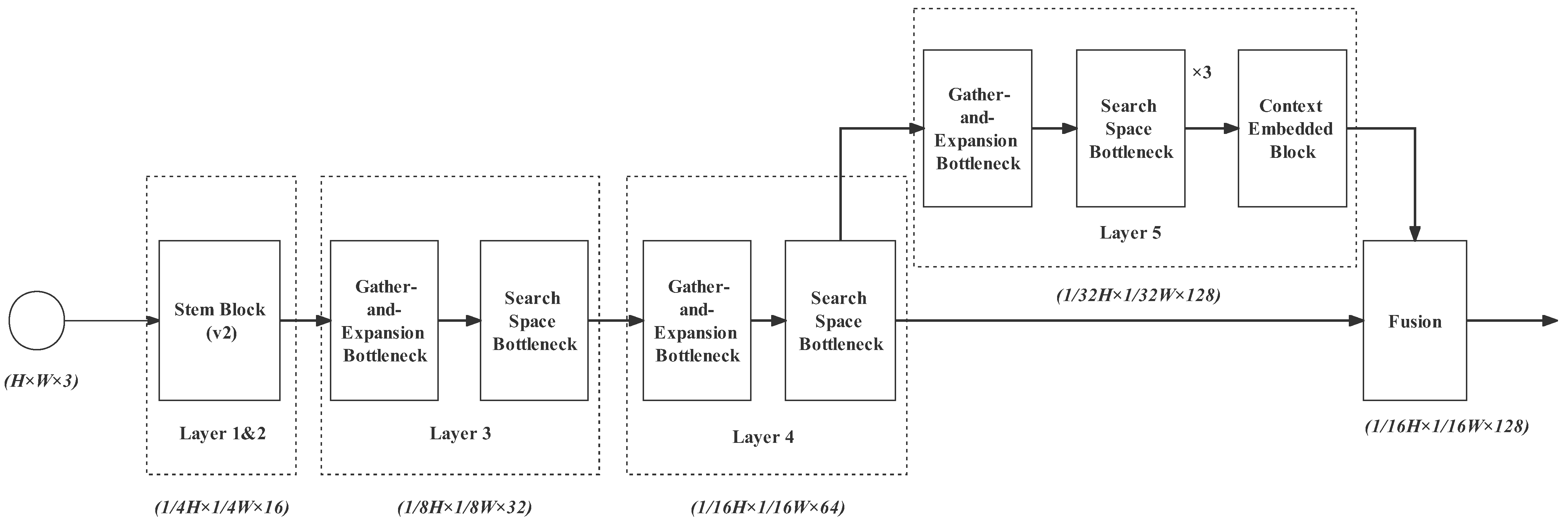
3.3. Semantic Path
- Layer 1 is a stem block we have introduced above. It shrinks the feature map size with a downsampling rate of 2 and enlarges the spatial slightly from 3 to 8 channels. With this layer, redundant information can be removed before complex computations;
- Layer 2 is as same as Layer 1, but it expands the channels from 8 to 16. The downsampling rate is 4;
- Gather–expand–search (GES) layers: Layers 3, 4, and 5, as well as the feature fusion layer constitute the GES layer. It mainly consists of a gather-and-expansion bottleneck and search-space bottlenecks. The gather-and-expansion bottleneck gathers feature representation by downsampling and storing spatial information by expanding channels. In each GES layer, a gather-and-expansion bottleneck is followed by several search-space bottlenecks. The search-space bottlenecks do not shrink the image size. They search for multi-resolution feature representations and integrate them. Detailed information for Layers 3, 4, 5 and the feature fusion layer is as follows:
- Layer 3: gather-and-expansion bottleneck + search-space bottleneck. The image channel is expanded to 32 and the downsampling rate is 8;
- Layer 4: The structure of Layer 4 is as same as Layer 2. Its output channel is 64 and the downsampling rate is 16;
- Layer 5: gather-and-expansion bottleneck + three search-space bottlenecks. In this layer, the output channel is 128, and the downsampling rate is 32. In the case of a high downsampling rate, plenty of search-space operations are particularly needed for enlarging the receptive field effectively. It can also further extract feature representation while maintaining the feature map size. In Layer 5, we also add the context-embedding block at the end to embed the global contextual information;
- The feature fusion layer is used for progressively aggregating the output feature of Layer 4 (downsampling rate of 16) and Layer 5 (downsampling rate of 32).
3.3.1. Gather–Expand–Search (GES) Layers with a Larger Receptive Field
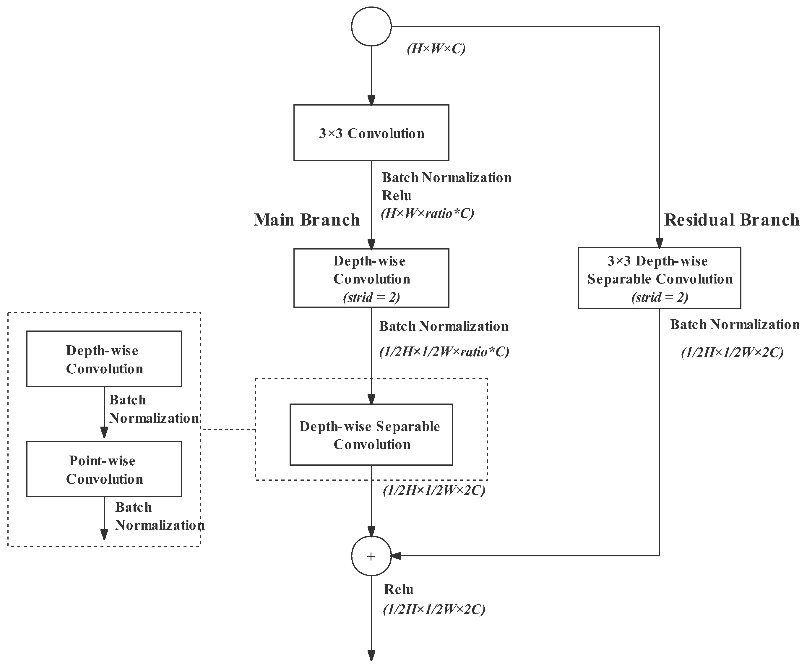
Gather-and-Expansion Bottleneck
- 3 × 3 standard convolution: The 3 × 3 standard convolution with a stride of 1 at the beginning plays the role of channel expansion. The channels can be expanded with arbitrary appropriate ratios, but the experimental results in the BiSeNetv2 paper proved that the ratio of 6 has the best performance. Therefore, we also retained the ratio of 6 in our design;
- Depth-wise convolution: Depth-wise convolution performs a 3 × 3 convolution for each channel, reducing computational complexity significantly. In the original design in BiSeNetv2, the depth-wise convolution is responsible for channel expansion. However, in our design, the depth-wise convolution at any position does not change the number of channels. Our experimental results (in Section 3) proved that it will make the feature representation more accurate. In the main branch, the depth-wises convolution has a stride of 2, downsampling the feature map to half of the input;
- Depth-wise separable convolution: This is composed of a depth-wise convolution followed by a point-wise convolution. The depth-wise convolution conducts convolution on each channel separably and then the individual channels are combined by a point-wise convolution. The point-wise convolution is a 1 × 1 convolution. The 1 × 1 convolution is flexible for changing dimensions; therefore, it is also used to project the feature map into a narrower space of twice the input channels. In the main branch, the depth-wise separable convolution does not shrink image size;
- Residual branch: The residual branch can restore the input information and protect the neural network from degradation [33]. In order to fuse with the main branch, the residual branch needs the same downsampling rate as the main branch. Therefore, a depth-wise separable convolution with a stride of 2 is performed in the residual branch. The downsampling operation is performed in the depth-wise convolution.
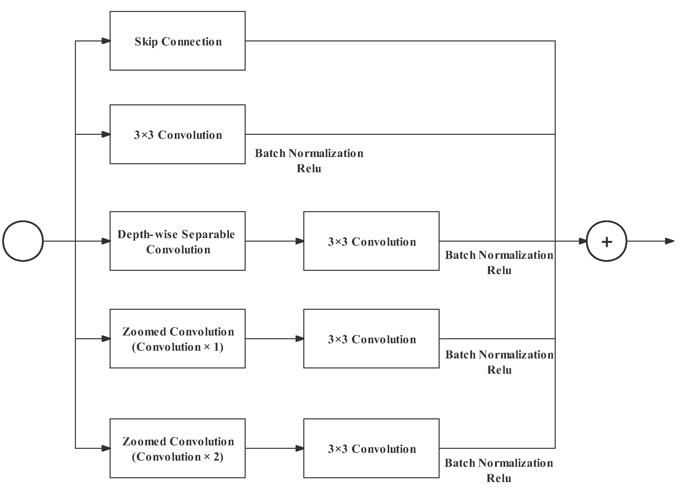
Search-Space Bottleneck
- Skip Connection: with this residual branch, more information can be utilized by subsequent blocks;
- A standard 3 × 3 convolution (with batch normalization and ReLU;.
- A depth-wise separable convolution followed by a standard 3 × 3 convolution. The structure of the depth-wise separable convolution is explained in the gather-and-expansion bottleneck;
- A zoomed convolution followed by a standard 3 × 3 convolution. The zoomed convolution here has one convolution in the middle (shown in Figure 7);
- Similar to Branch 4, but the zoomed convolution here has two convolutions (shown in Figure 8).
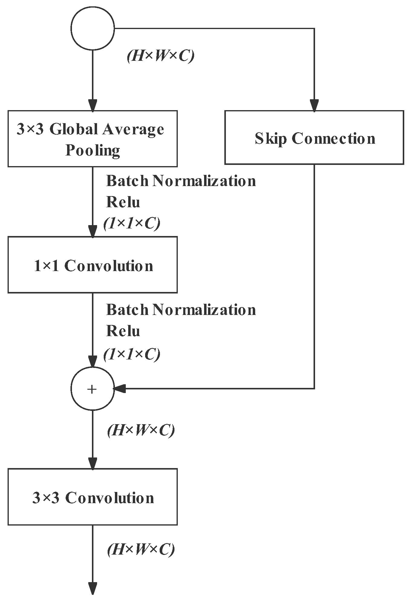
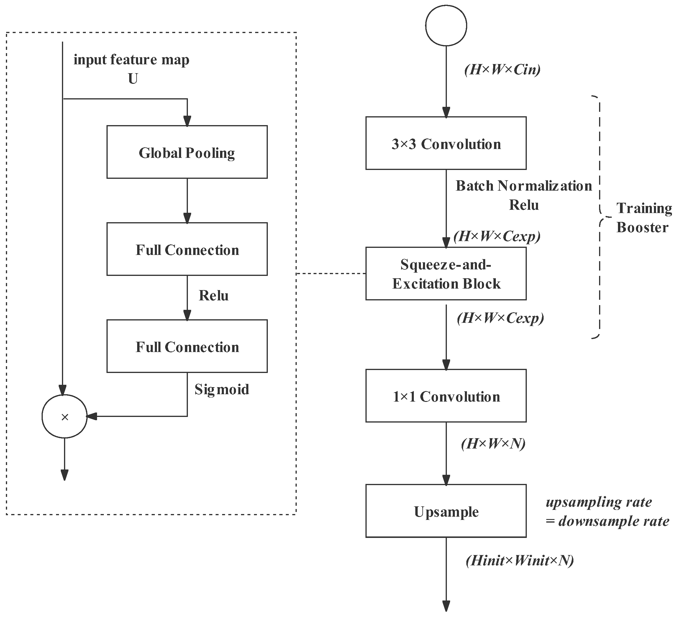
Context-Embedding Block
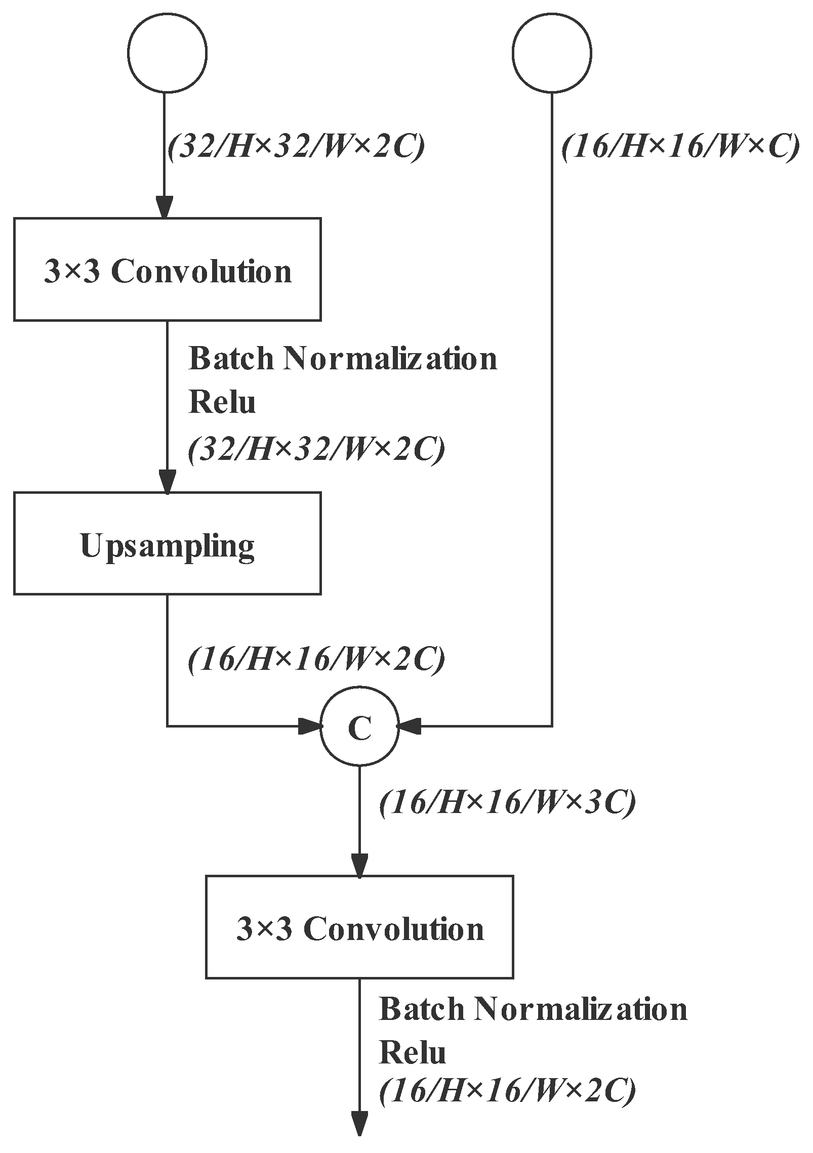
Feature Fusion
3.4. Detail Path
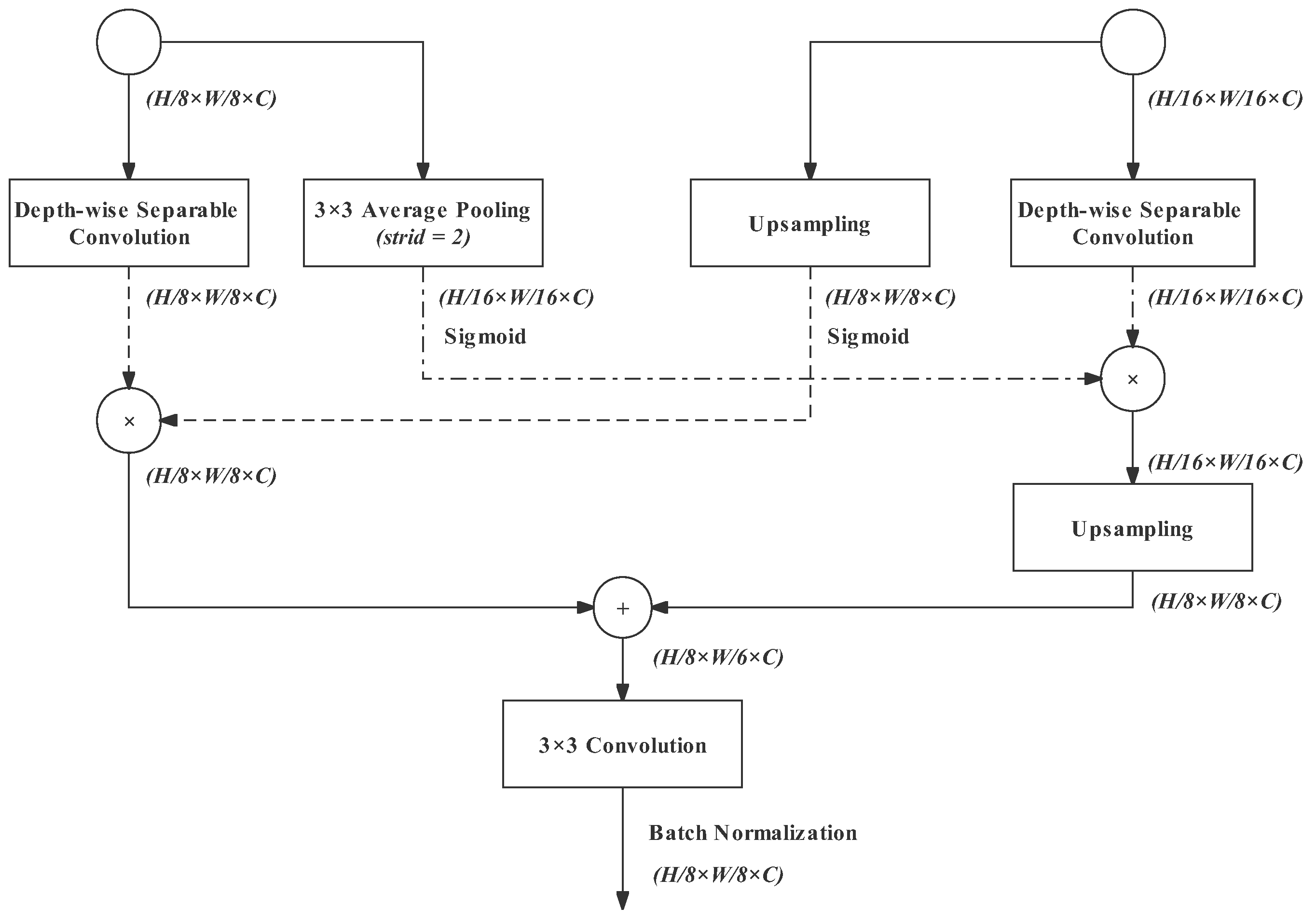
3.5. Bilateral Guided Aggregation
- Left Branch 1: A depth-wise separable convolution for further gathering feature representation fast;
- Left Branch 2: Average pooling with a stride of 2 results in a 16 downsampling rate. Its output will be fused with the output of the semantic path;
- Right Branch 1: The upsampling operation restores the output of the semantic path to an downsampling rate of 8. Its output will be fused with the output of detail path;
- Right Branch 2: Its structure and effect are as same as Left Branch 1.
3.6. Segment Head with Training Boosting Strategy
3.6.1. Segment Head
3.6.2. Training Boosting Strategy
4. Experimental Results
4.1. Benchmark Dataset
4.2. Training Details
4.2.1. General Training Settings
4.2.2. Cost Function
4.2.3. Image Augmentation
- Randomly scale the image size. The scale value ranged from 0.25 to 2.0;
- Randomly horizontally flip the images;
- Randomly change the color jitter. The brightness was 0.4, the contrast was 0.4 and the saturation was 0.4.
4.2.4. Inference Details
4.3. Hardware Support
4.4. Component Evaluation
4.4.1. Semantic Path
Design of Gather-and-Expansion Bottleneck
Design of Search-Space Bottleneck
Design of Feature Fusion
4.4.2. Design of Stem Block
4.4.3. Design of Detail Path
4.4.4. Design of Bilateral Guided Aggregation
4.4.5. Design of Training Booster Strategy
4.4.6. Ablation Results Summary
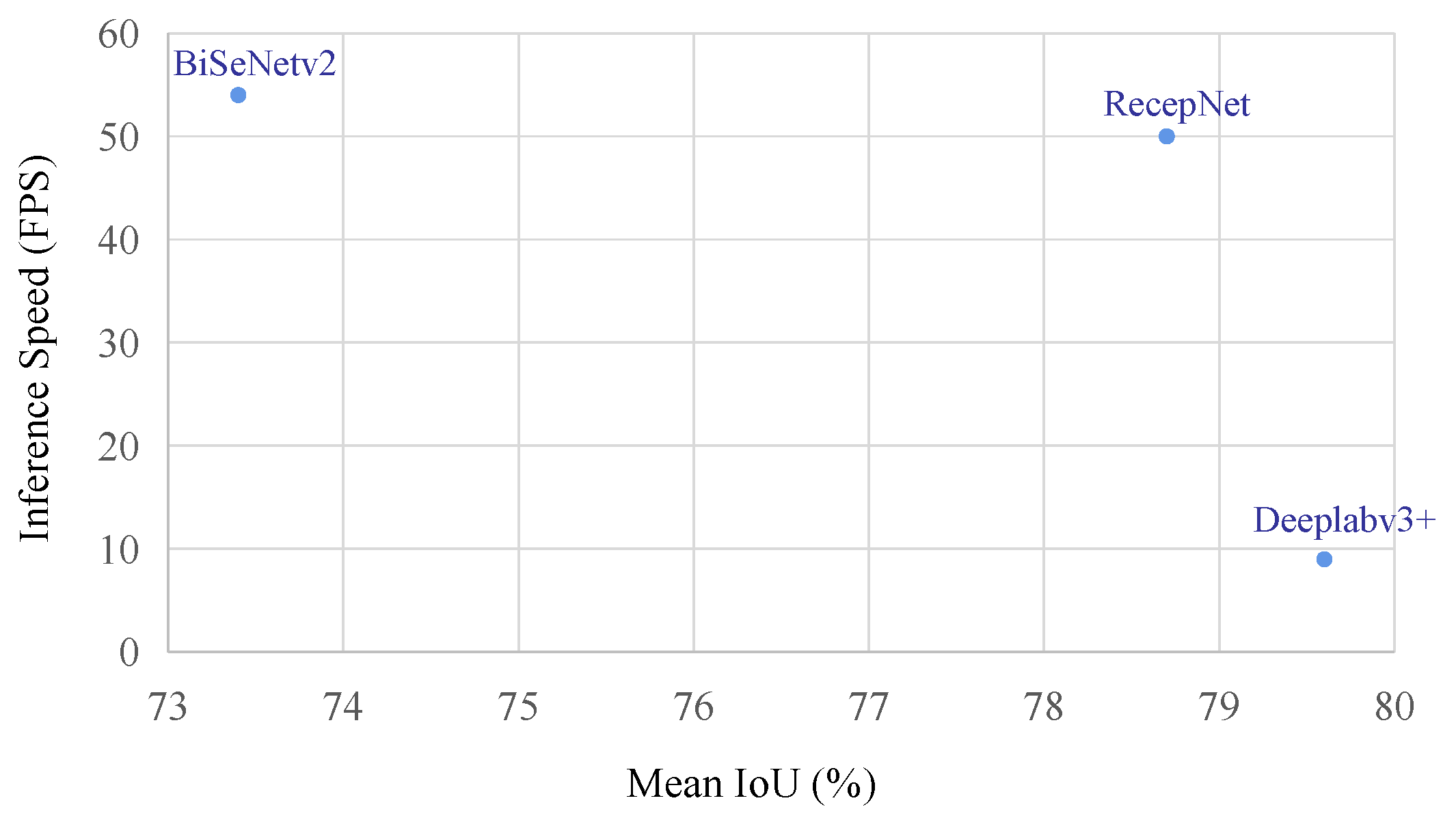
4.5. Inference Speed
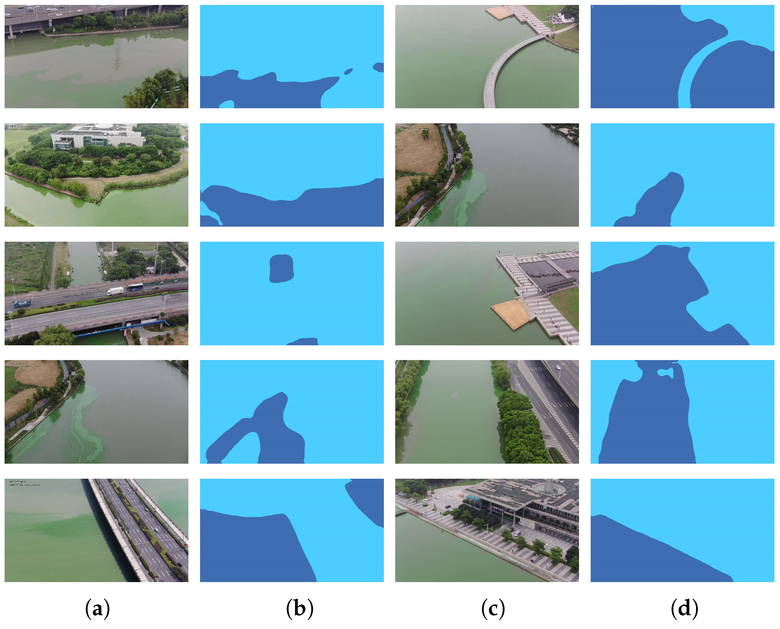
5. Application in Blue-Green Algae Detection
5.1. Blue-Green Algae Dataset
5.2. Network Performance on Blue-Green Algae Dataset
6. Conclusions
Author Contributions
Funding
Data Availability Statement
Acknowledgments
Conflicts of Interest
References
- Kang, Y.; Yamaguchi, K.; Naito, T.; Ninomiya, Y. Multiband Image Segmentation and Object Recognition for Understanding Road Scenes. IEEE Trans. Intell. Transp. Syst. 2011, 12, 1423–1433. [Google Scholar] [CrossRef]
- Chen, B.; Gong, C.; Yang, J. Importance-Aware Semantic Segmentation for Autonomous Vehicles. IEEE Trans. Intell. Transp. Syst. 2019, 20, 137–148. [Google Scholar] [CrossRef]
- Zeng, D.; Chen, X.; Zhu, M.; Goesele, M.; Kuijper, A. Background Subtraction With Real-Time Semantic Segmentation. IEEE Access 2019, 7, 153869–153884. [Google Scholar] [CrossRef]
- Simonyan, K.; Zisserman, A. Very deep convolutional networks for large-scale image recognition. arXiv 2014, arXiv:1409.1556. [Google Scholar]
- He, K.; Zhang, X.; Ren, S.; Sun, J. Deep residual learning for image recognition. In Proceedings of the IEEE Conference on Computer Vision and Pattern Recognition, Las Vegas, NV, USA, 27–30 June 2016; pp. 770–778. [Google Scholar]
- Chen, L.C.; Zhu, Y.; Papandreou, G.; Schroff, F.; Adam, H. Encoder-Decoder with Atrous Separable Convolution for Semantic Image Segmentation. arXiv 2018, arXiv:1802.02611. [Google Scholar]
- Paszke, A.; Chaurasia, A.; Kim, S.; Culurciello, E. ENet: A Deep Neural Network Architecture for Real-Time Semantic Segmentation. arXiv 2016, arXiv:1606.02147. [Google Scholar]
- Treml, M.; Arjona-Medina, J.; Unterthiner, T.; Durgesh, R.; Friedmann, F.; Schuberth, P.; Mayr, A.; Heusel, M.; Hofmarcher, M.; Widrich, M.; et al. Speeding up semantic segmentation for autonomous driving. In Proceedings of the MLITS, NIPS Workshop, Barcelona, Spain, 1 October 2016. [Google Scholar]
- Lin, G.; Milan, A.; Shen, C.; Reid, I. Refinenet: Multi-path Refinement Networks for High-Resolution Semantic Segmentation. In Proceedings of the IEEE Conference on Computer Vision and Pattern Recognition, Honolulu, HI, USA, 21–26 July 2017; pp. 1925–1934. [Google Scholar]
- Yu, C.; Gao, C.; Wang, J.; Yu, G.; Shen, C.; Sang, N. BiSeNet V2: Bilateral Network with Guided Aggregation for Real-time Semantic Segmentation. arXiv 2020, arXiv:2004.02147. [Google Scholar] [CrossRef]
- Otsu, N. A Threshold Selection Method from Gray-Level Histograms. IEEE Trans. Syst. Man Cybern. 1979, 9, 62–66. [Google Scholar] [CrossRef] [Green Version]
- Mottaghi, R.; Chen, X.; Liu, X.; Cho, N.G.; Lee, S.W.; Fidler, S.; Urtasun, R.; Yuille, A. The Role of Context for Object Detection and Semantic Segmentation in the Wild. In Proceedings of the IEEE Conference on Computer Vision and Pattern Recognition, Columbus, OH, USA, 23–28 June 2014; pp. 891–898. [Google Scholar]
- Shotton, J.; Winn, J.; Rother, C.; Criminisi, A. Textonboost for Image Understanding: Multi-class Object Recognition and Segmentation by Jointly Modeling Texture, Layout, and Context. Int. J. Comput. Vis. 2009, 81, 2–23. [Google Scholar] [CrossRef] [Green Version]
- Achanta, R.; Shaji, A.; Smith, K.; Lucchi, A.; Fua, P.; Süsstrunk, S. SLIC Superpixels Compared to State-of-the-Art Superpixel Methods. IEEE Trans. Pattern Anal. Mach. Intell. 2012, 34, 2274–2282. [Google Scholar] [CrossRef] [Green Version]
- Kalchbrenner, N.; Grefenstette, E.; Blunsom, P. A Convolutional Neural Network for Modelling Sentences. In Proceedings of the 52nd Annual Meeting of the Association for Computational Linguistics (Volume 1: Long Papers); Association for Computational Linguistics: Baltimore, MD, USA, 2014; pp. 655–665. [Google Scholar] [CrossRef] [Green Version]
- Long, J.; Shelhamer, E.; Darrell, T. Fully Convolutional Networks for Semantic Segmentation. arXiv 2015, arXiv:1411.4038. [Google Scholar]
- Chen, L.C.; Papandreou, G.; Kokkinos, I.; Murphy, K.; Yuille, A.L. Semantic Image Segmentation with Deep Convolutional Nets and Fully Connected CRFs. arXiv 2016, arXiv:1412.7062. [Google Scholar]
- Chen, L.C.; Papandreou, G.; Kokkinos, I.; Murphy, K.; Yuille, A.L. Deeplab: Semantic Image Segmentation with Deep Convolutional Nets, Atrous Convolution, and Fully Connected Crfs. IEEE Trans. Pattern Anal. Mach. Intell. 2017, 40, 834–848. [Google Scholar] [CrossRef] [PubMed] [Green Version]
- Zhao, H.; Shi, J.; Qi, X.; Wang, X.; Jia, J. Pyramid Scene Parsing Network. arXiv 2017, arXiv:1612.01105. [Google Scholar]
- Yuan, Y.; Wang, J. Ocnet: Object Context Network for Scene Parsing. arXiv 2018, arXiv:1809.00916. [Google Scholar]
- Zhao, H.; Zhang, Y.; Liu, S.; Shi, J.; Loy, C.C.; Lin, D.; Jia, J. Psanet: Point-wise Spatial Attention Network for Scene Parsing. In Proceedings of the European Conference on Computer Vision (ECCV), Munich, Germany, 8–14 September 2018; pp. 267–283. [Google Scholar]
- Ronneberger, O.; Fischer, P.; Brox, T. U-Net: Convolutional Networks for Biomedical Image Segmentation. In Proceedings of the International Conference on Medical Image Computing and Computer-Assisted Intervention, Munich, Germany, 5–9 October 2015; Springer: Berlin/Heidelberg, Germany, 2015; pp. 234–241. [Google Scholar]
- Yu, C.; Wang, J.; Peng, C.; Gao, C.; Yu, G.; Sang, N. Learning a Discriminative Feature Network for Semantic Segmentation. In Proceedings of the IEEE Conference on Computer Vision and Pattern Recognition, Salt Lake City, UT, USA, 23–28 June 2018; pp. 1857–1866. [Google Scholar]
- Wang, J.; Sun, K.; Cheng, T.; Jiang, B.; Deng, C.; Zhao, Y.; Liu, D.; Mu, Y.; Tan, M.; Wang, X.; et al. Deep High-Resolution Representation Learning for Visual Recognition. IEEE Trans. Pattern Anal. Mach. Intell. 2020, 43, 3349–3364. [Google Scholar] [CrossRef]
- Zheng, S.; Jayasumana, S.; Romera-Paredes, B.; Vineet, V.; Su, Z.; Du, D.; Huang, C.; Torr, P.H. Conditional Random Fields as Recurrent Neural Networks. In Proceedings of the IEEE International Conference on Computer Vision, Washington, DC, USA, 7–13 December 2015; pp. 1529–1537. [Google Scholar]
- Mehta, S.; Rastegari, M.; Caspi, A.; Shapiro, L.; Hajishirzi, H. Espnet: Efficient Spatial Pyramid of Dilated Convolutions for Semantic Segmentation. In Proceedings of the European Conference on Computer Vision (ECCV), Munich, Germany, 8–14 September 2018; pp. 552–568. [Google Scholar]
- Romera, E.; Alvarez, J.M.; Bergasa, L.M.; Arroyo, R. Erfnet: Efficient Residual Factorized Convnet for Real-Time Semantic Segmentation. IEEE Trans. Intell. Transp. Syst. 2017, 19, 263–272. [Google Scholar] [CrossRef]
- Zhao, H.; Qi, X.; Shen, X.; Shi, J.; Jia, J. Icnet for Real-Time Semantic Segmentation on High-Resolution Images. In Proceedings of the European Conference on Computer Vision (ECCV), Munich, Germany, 8–14 September 2018; pp. 405–420. [Google Scholar]
- Wang, Y.; Zhou, Q.; Liu, J.; Xiong, J.; Gao, G.; Wu, X.; Latecki, L.J. Lednet: A Lightweight Encoder-Decoder Network for Real-Time Semantic Segmentation. In Proceedings of the 2019 IEEE International Conference on Image Processing (ICIP), Taipei, Taiwan, 22–25 September 2019; pp. 1860–1864. [Google Scholar]
- Sandler, M.; Howard, A.; Zhu, M.; Zhmoginov, A.; Chen, L.C. MobileNetV2: Inverted Residuals and Linear Bottlenecks. arXiv 2019, arXiv:1801.04381. [Google Scholar]
- Zhang, X.; Zhou, X.; Lin, M.; Sun, J. Shufflenet: An Extremely Efficient Convolutional Neural Network for Mobile Devices. In Proceedings of the IEEE Conference on Computer Vision and Pattern Recognition, Salt Lake City, UT, USA, 18–22 June 2018; pp. 6848–6856. [Google Scholar]
- Chen, W.; Gong, X.; Liu, X.; Zhang, Q.; Li, Y.; Wang, Z. FasterSeg: Searching for Faster Real-time Semantic Segmentation. arXiv 2020, arXiv:1912.10917. [Google Scholar]
- Wu, D.; Wang, Y.; Xia, S.T.; Bailey, J.; Ma, X. Skip Connections Matter: On the Transferability of Adversarial Examples Generated with Resnets. arXiv 2020, arXiv:2002.05990. [Google Scholar]
- Liu, C.; Chen, L.C.; Schroff, F.; Adam, H.; Hua, W.; Yuille, A.; Li, F.-F. Auto-DeepLab: Hierarchical Neural Architecture Search for Semantic Image Segmentation. arXiv 2019, arXiv:1901.02985. [Google Scholar]
- Hu, J.; Shen, L.; Albanie, S.; Sun, G.; Wu, E. Squeeze-and-Excitation Networks. arXiv 2019, arXiv:1709.01507. [Google Scholar]
- Cordts, M.; Omran, M.; Ramos, S.; Rehfeld, T.; Enzweiler, M.; Benenson, R.; Franke, U.; Roth, S.; Schiele, B. The Cityscapes Dataset for Semantic Urban Scene Understanding. In Proceedings of the IEEE Conference on Computer Vision and Pattern Recognition, Las Vegas, NV, USA, 26 June–1 July 2016; pp. 3213–3223. [Google Scholar]
- Rahman, M.A.; Wang, Y. Optimizing intersection-over-union in deep neural networks for image segmentation. In Proceedings of the International Symposium on Visual Computing, Las Vegas, NV, USA, 12–14 December 2016; Springer: Berlin/Heidelberg, Germany, 2016; pp. 234–244. [Google Scholar]
- Biswas, A.; Chandrakasan, A.P. CONV-SRAM: An energy-efficient SRAM with in-memory dot-product computation for low-power convolutional neural networks. IEEE J. Solid-State Circuits 2018, 54, 217–230. [Google Scholar] [CrossRef] [Green Version]
- Paszke, A.; Gross, S.; Massa, F.; Lerer, A.; Bradbury, J.; Chanan, G.; Killeen, T.; Lin, Z.; Gimelshein, N.; Antiga, L.; et al. Pytorch: An Imperative Style, High-Performance Deep Learning Library. Adv. Neural Inf. Process. Syst. 2019, 32, 8026–8037. [Google Scholar]
- Sarhadi, A.; Burn, D.H.; Johnson, F.; Mehrotra, R.; Sharma, A. Water resources climate change projections using supervised nonlinear and multivariate soft computing techniques. J. Hydrol. 2016, 536, 119–132. [Google Scholar] [CrossRef] [Green Version]
- Sadeghifar, T.; Lama, G.; Sihag, P.; Bayram, A.; Kisi, O. Wave height predictions in complex sea flows through soft-computing models: Case study of Persian Gulf. Ocean. Eng. 2022, 245, 110467. [Google Scholar] [CrossRef]
- Lama, G.; Errico, A.; Pasquino, V.; Mirzaei, S.; Preti, F.; Chirico, G. Velocity Uncertainty Quantification based on Riparian Vegetation Indices in open channels colonized by Phragmites australis. J. Ecohydraulics 2022, 7, 71–76. [Google Scholar] [CrossRef]
- Vu, H.P.; Nguyen, L.N.; Zdarta, J.; Nga, T.T.; Nghiem, L.D. Blue-Green Algae in Surface Water: Problems and Opportunities. Curr. Pollut. Rep. 2020, 6, 105–122. [Google Scholar] [CrossRef]
- Hu, Z.; Luo, W. Method for Detecting Water Body Blue Algae Based on PCR-DCG and Kit Thereof. China Patent CN101701264B, 28 December 2011. [Google Scholar]


| Stage | opr | k | s | c | Downsampling Rate | |
|---|---|---|---|---|---|---|
| Detail Path | Stage 1 | Stem | 3 | 2 | 32 | 2 |
| SepConv | 3 | 1 | 32 | |||
| Stage 1 | Stem | 3 | 2 | 64 | 4 | |
| SepConv | 3 | 1 | 64 | |||
| Conv | 3 | 1 | 64 | |||
| Stage 1 | Stem | 3 | 2 | 128 | 8 | |
| SepConv | 3 | 1 | 128 | |||
| Conv | 3 | 1 | 128 |
| Stage | opr | k | s | c | Downsampling Rate | ||
|---|---|---|---|---|---|---|---|
| Semantic Path | Layer 1 | Stem | 3 | 2 | 8 | 2 | |
| Layer 2 | Stem | 3 | 2 | 16 | 4 | ||
| GES | Layer 3 | GE | 3 | 2 | 32 | ||
| SS | 3 | 1 | 32 | 8 | |||
| Layer 4 | GE | 3 | 2 | 64 | |||
| SS | 3 | 1 | 64 | 16 | |||
| Layer 5 | GE | 3 | 2 | 128 | |||
| SS | 3 | 1 | 128 | ||||
| SS | 3 | 1 | 128 | ||||
| SS | 3 | 1 | 128 | ||||
| CE | 3 | 1 | 128 | 32 | |||
| Feature Fusion | Fusion | - | - | 128 | 16 | ||
| Network | GMACs | % mIoU |
|---|---|---|
| Semantic branch of BiSeNetv2 | 4.38 | 65.11 |
|
Semantic branch of BiSeNetv2 (replace inverted bottleneck (strid = 2) with our GE bottleneck) | 4.40 | 65.27 |
| Network | Structure of Zoomed Convolution | GMACs | % mIoU | ||
|---|---|---|---|---|---|
| Bilinear Downsample | Feature-Extraction Operation | Bilinear Upsample | |||
| Network for search-space bottleneck testing | ✓ | 3 × 3 conv | ✓ | 4.97 | 60.42 |
| ✓ | 3 × 3 conv + 3 × 3conv | ✓ | 5.67 | 62.53 | |
| ✓ | 3 × 3 conv + 1 × 1 conv | ✓ | 6.33 | 61.28 | |
| ✓ | 3 × 3 conv + depth-wise separable convolution | ✓ | 5.23 | 62.50 | |
| Network | Branches of Search-Space Bottleneck | GMACs | % mIoU | ||||
|---|---|---|---|---|---|---|---|
| Skip | 3 × 3 conv | SepConv + 3 × 3 conv | ZoomedConv (conv ×1) + 3 × 3 conv | ZoomedConv (conv × 2) + 3 × 3 conv | |||
| Network for search-space bottleneck Testing | ✓ | ✓ | ✓ | ✓ | 4.21 | 63.78 | |
| ✓ | ✓ | ✓ | ✓ | 3.83 | 67.73 | ||
| ✓ | ✓ | ✓ | ✓ | 3.79 | 67.96 | ||
| ✓ | ✓ | ✓ | ✓ | 3.77 | 67.45 | ||
| ✓ | ✓ | ✓ | ✓ | 3.72 | 67.38 | ||
| ✓ | ✓ | ✓ | ✓ | ✓ | 4.02 | 68.21 | |
|
Semantic path in BiSeNetv2 | 4.38 | 65.11 | |||||
| Network | GMACs | % mIoU |
|---|---|---|
|
Network for feature fusion testing | 4.05 | 69.39 |
| Network for search-space bottleneck testing | 4.02 | 68.21 |
| Semantic branch of BiSeNetv2 (with our GE bottleneck) | 4.38 | 65.11 |
| Network | GMACs | % mIoU |
|---|---|---|
| Semantic path of RecepNet | 4.08 | 69.61 |
| Network for feature fusion testing | 4.05 | 69.39 |
| Semantic branch of BiSeNetv2 | 4.38 | 65.11 |
| Network | GMACs | % mIoU |
|---|---|---|
| Detail branch of BiSeNetv2 | 11.72 | 62.35 |
| Detail b of RecepNet | 9.58 | 65.30 |
| Network | GMACs | % mIoU |
|---|---|---|
| BiSeNetv2 without booster | 14.83 | 69.67 |
| RecepNet without booster | 15.21 | 74.81 |
| Network | GMACs | % mIoU |
|---|---|---|
| RecepNet without booster | 15.21 | 74.81 |
|
RecepNet with booster in BiSeNetV2 | 15.21 | 78.03 |
| RecepNet | 15.21 | 78.65 |
| BiSeNetv2 | 14.83 | 73.36 |
| Components | GMACs (Complexity) | % mIoU (Accuracy) | |||||
|---|---|---|---|---|---|---|---|
| Detail | Semantic | Aggregation | Booster | RecepNet | BiSeNetV2 | RecepNet | BiSeNetV2 |
| ✓ | 9.58 | 11.72 | 65.30 | 62.35 | |||
| ✓ | 4.02 | 4.38 | 68.21 | 65.11 | |||
| ✓ | ✓ | ✓ | 15.21 | 14.83 | 74.81 | 69.67 | |
| ✓ | ✓ | ✓ | ✓ | 15.21 | 14.83 | 78.65 | 73.36 |
| Network | % mIoU | GAMCs |
|---|---|---|
| BiSeNetv2 | 79.51 | 51.72 |
| RecepNet | 82.12 | 52.12 |
| DeepLabv3+ | 83.36 | 55.52 |
Publisher’s Note: MDPI stays neutral with regard to jurisdictional claims in published maps and institutional affiliations. |
© 2022 by the authors. Licensee MDPI, Basel, Switzerland. This article is an open access article distributed under the terms and conditions of the Creative Commons Attribution (CC BY) license (https://creativecommons.org/licenses/by/4.0/).
Share and Cite
Yang, K.; Wang, Z.; Yang, Z.; Zheng, P.; Yao, S.; Zhu, X.; Yue, Y.; Wang, W.; Zhang, J.; Ma, J. RecepNet: Network with Large Receptive Field for Real-Time Semantic Segmentation and Application for Blue-Green Algae. Remote Sens. 2022, 14, 5315. https://doi.org/10.3390/rs14215315
Yang K, Wang Z, Yang Z, Zheng P, Yao S, Zhu X, Yue Y, Wang W, Zhang J, Ma J. RecepNet: Network with Large Receptive Field for Real-Time Semantic Segmentation and Application for Blue-Green Algae. Remote Sensing. 2022; 14(21):5315. https://doi.org/10.3390/rs14215315
Chicago/Turabian StyleYang, Kaiyuan, Zhonghao Wang, Zheng Yang, Peiyang Zheng, Shanliang Yao, Xiaohui Zhu, Yong Yue, Wei Wang, Jie Zhang, and Jieming Ma. 2022. "RecepNet: Network with Large Receptive Field for Real-Time Semantic Segmentation and Application for Blue-Green Algae" Remote Sensing 14, no. 21: 5315. https://doi.org/10.3390/rs14215315