
Comparison of Three Convolution Neural Network Schemes to Retrieve Temperature and Humidity Profiles from the FY4A GIIRS Observations
Collaborative Innovation Center on Forecast and Evaluation of Meteorological Disasters, Key Laboratory for Aerosol-Cloud-Precipitation of China Meteorological Administration, Nanjing University of Information Science and Technology, Nanjing 210044, China
*
Author to whom correspondence should be addressed.
Remote Sens. 2022, 14(20), 5112; https://doi.org/10.3390/rs14205112
Submission received: 26 August 2022
/
Revised: 29 September 2022
/
Accepted: 10 October 2022
/
Published: 13 October 2022
(This article belongs to the Topic A Themed Issue in Memory of Academician Duzheng Ye (1916–2013))
Abstract
:FY4A/GIIRS (Geostationary Interferometric Infrared Sounder) is the first infrared hyperspectral atmospheric vertical sounder onboard a geostationary satellite. It can achieve observations of atmospheric temperature and humidity profiles with high vertical and temporal resolutions. Presently, convolutional neural network algorithms are relatively less used in the field of atmospheric profile retrieval, and different convolutional neural network approaches have different characteristics. The one-dimensional convolutional neural network scheme 1D-Net and two three-dimensional retrieval schemes U-Net 1 and U-Net 2 are used to achieve atmospheric temperature and humidity profiles under all skies based on GIIRS-observed brightness temperatures in this paper. After validation with test training data, the retrievals of different schemes derived from actual GIIRS observations and level 2 operational products were verified with ERA5 reanalysis data and radiosonde measurements in summer and winter respectively. The retrieved three-dimensional temperature and humidity fields from U-Net 1 and U-Net 2 are closer to the ERA5 reanalysis field in both distribution and value than the retrievals from the 1D-Net scheme and level 2 operational products. In particular, the inversion field of the U-Net 2 scheme is more continuous in space. Compared with radiosonde observations, the accuracy of the level 2 temperature product is the highest when the field of view is completely clear both in winter and summer month. The root mean square error (RMSE) of temperature retrieval of the two U-Net schemes is the second highest, and the RMSE and bias of the 1D-Net scheme are both large. Two U-Net schemes overestimate the temperature and humidity slightly in winter and underestimate it in summer in both clear and all sky cases. Under all sky conditions, the temperature retrieval RMSE and bias of the two U-Net schemes above 800 hPa are lower than those of the level 2 products, especially the U-Net 2 scheme with an RMSE of approximately 2.5 K. The U-Net 2 scheme bias is the smallest, with a value of approximately 0.5 K in winter. Since the level 2 product only provides the atmospheric temperature above the cloud top, it indicates that its temperature product accuracy is very low when the field of view is influenced by clouds. The humidity retrieval RMSEs of the two U-Net schemes is within 2 g/kg, better than that of the 1D-Net scheme. The retrieval accuracy of the U-Net 2 scheme is approximately 0.3 g/kg better than that of the U-Net 1 scheme below 600 hPa in winter. Level 2 does not provide humidity products. The summer humidity retrieval is worse than in winter. In general, among the three deep machine learning algorithms, 1D-Net has a large retrieval error, and the temperature and humidity from U-Net 2 have the highest accuracy. The retrieval speeds of the two U-Net schemes are nearly the same, and both are faster than that of scheme 1D-Net.
1. Introduction
Atmospheric temperature and humidity profiles are two important parameters to study atmospheric state and play an important role in the research of atmospheric science. Accurately obtaining these parameters is of great significance to improve the accuracy of numerical weather forecast and short-term weather warning and forecast [1]. The traditional way of obtaining atmospheric temperature and humidity profiles through radiosonde observations has limited spatial representativeness due to the influence of geographical conditions and other factors and has failed to meet the needs of operational and modern meteorological development. However, the development of satellite remote sensing technology has made up for the shortage of radiosondes and provided technical support for the acquisition of global atmospheric temperature and humidity profile distributions with high spatial-temporal resolution [2].
The horizontal and vertical resolutions and accuracies of atmospheric temperature and humidity profiles must meet the requirements of numerical weather prediction systems, so it is necessary to study the remote sensing accuracy that can be achieved by using satellite technology and to study which retrieval method can obtain the optimal retrieval results. The number of setting channels for atmospheric sounding radiometers uploaded on meteorological satellite platforms determines their vertical observation resolution. Due to the small number of channels, the spectral resolution of microwave and imager instruments is low, and the weight function is too wide, so it is impossible to retrieve the fine atmospheric profile in the vertical direction. In contrast, the spaceborne infrared hyperspectral atmospheric vertical sounders have thousands of channels in the thermal infrared band with high spectral resolution and narrow weighting function and can obtain high vertical resolution three-dimensional finer observations of atmospheric temperature and humidity parameters.
The Geostationary Interferometric Infrared Sounder (GIIRS) onboard FY-4A launched on 11 December 2016 (China’s new generation of quantitative remote sensing meteorological satellites with geostationary orbits) is the first infrared hyperspectral atmospheric sounder mounted on a geostationary meteorological satellite. The GIIRS can provide time-continuous, high-spectral-resolution atmospheric sounding information [3], which is used to retrieve the vertical structure of atmospheric temperature and humidity parameters with high vertical resolution. The improved vertical resolution provides higher accuracy services for numerical weather forecasting, weather monitoring, and warning [4].
To date, the traditional methods commonly used to retrieve atmospheric temperature and humidity profiles based on satellite-based infrared hyperspectral observations are statistical regression methods and physical retrieval methods. The statistical regression approaches include the eigenvector method [5,6,7], empirical orthogonal function expansion method [8], and least squares method. Although the statistical regression algorithm is simple to calculate and retrieval results are more stable, it does not consider the physical nature of the atmospheric radiation transmission process, and the retrieval accuracy needs to be improved. Moreover, the method relies on training samples and cannot be applied to areas where the sample information is not sufficiently representative. Although the retrieval accuracy is high, the physical retrieval method, such as the one-dimensional variational method, requires an initial field, complex physical processes to be considered, and a long computation time [9,10].
With the continuous development of artificial intelligence, machine learning algorithms have been applied to various research fields and have demonstrated a powerful ability to handle big data. Machine learning algorithms with features such as adaptive, self-organizing, and real-time learning have gradually been introduced into the field of meteorology, providing new ideas for atmospheric remote sensing. Singh et al. [11] retrieved atmospheric temperature and humidity profiles from microwave and infrared hyperspectral data, respectively, with a shallow learning neural network approach, and the results showed good agreement for all atmospheric pressure levels except for below 850 hPa. The deep learning algorithm is now also gradually applied to satellite remote sensing retrieval with the continuous development of machine learning. For example, Malmgren-Hansen et al. retrieved atmospheric temperature profiles with a convolutional neural network (CNN) algorithm based on infrared atmospheric sounding interferometer (IASI) observations and found that the CNN algorithm has higher retrieval accuracy than the linear regression method [12].
As one of the representative methods of deep machine learning (namely, hierarchical machine learning methods including multilevel nonlinear transformations), the convolutional neural network algorithm mainly integrates feature extraction into multilayer perceptions through structural reorganization and weight reduction. It unifies feature representation and regression prediction with obvious advantages compared to shallow models in feature extraction and modelling and has achieved good performance in image recognition and classification [13,14,15]. However, its application in the field of atmospheric parameter profile retrieval has rarely been reported in the literature. Therefore, three convolutional neural network schemes are applied to retrieve atmospheric temperature and humidity profiles based on the infrared hyperspectral GIIRS observations in this paper, namely, the traditional convolutional neural network scheme 1D-Net to retrieve the one-dimensional atmospheric temperature and humidity profiles and the U-Net 1 and U-Net 2 schemes to retrieve the three-dimensional profiles. Meanwhile, the retrieval accuracy and efficiency of each scheme are evaluated by comparison and verification.
2. Data
2.1. GIIRS Data
GIIRS is the first hyperspectral infrared instrument onboard the geostationary meteorological satellite, and two infrared spectral bands (longwavelength IR (LWIR) band of 700–1130 and the medium-wavelength IR (MWIR) band of 1650–2250 ) with a spectral resolution of 0.625 are designed to detect the atmosphere. There are 1650 channels in total, and the nadir spatial resolution is 16 km. The LWIR band is 689 channels containing the absorption band near 15 μm, the thermal infrared window region in the 8–12 μm and the 9.6 μm absorption band. The MWIR band includes the strong water vapor absorption band (5–8 μm) centered at 6.3 μm, which can be used to retrieve atmospheric water vapor profiles, as well as the absorption band near 4.3 μm, with a total of 961 channels. The main GIIRS instrument performance parameters are given in Table 1. GIIRS observes China and its surrounding area (3°~55°N, 66°~144°E), including 7 latitude belts from north to south, with each belt taking 15 min. Each scan belt has 59 fields of regard (FORs), and each FOR contains 128 fields of view (FOVs). Each GIIRS FOR is composed of 128 FOVs arranged in a 32 4 array.
GIIRS Level 1 (L1) radiation observed data for the whole month of February 2020 and February 2021 were used in this study, including radiance measurement, latitude, longitude, and satellite zenith angle information. At the same time, cloud mask (CLM) and atmospheric temperature profile products from GIIRS Level 2 (L2) operational products were used. The GIIRS L1 and L2 datasets are from the Chinese National Satellite Meteorological Center (http://satellite.nsmc.org.cn, accessed on 12 January 2022).
2.2. ERA5 Reanalysis Data
European Centre for Medium-Range Weather Forecasts (ECMWF) consistently generates atmospheric reanalyses of the global climate by assimilating various data from the ground, upper air, and satellite observations into the earth system model [16]. The ERA5 dataset (https://apps.ecmwf.int/datasets/, accessed on 12 January 2022) is the latest generation reanalysis dataset provided by the ECMWF, which makes a significant step forward in the assimilation system, model input, spatial resolution, output frequency, and quality level compared with its former ERA-Interim [17]. The spatial resolution is 0.25° 0.25°, and the temporal resolution is 1 h. There are 37 pressure levels from 1000 hPa to 1 hPa. The atmospheric temperature and water vapor parameters of the three-dimensional grid are mainly used for validation. Since the ERA5 data and GIIRS observations are different in spatial and temporal resolution, the ERA5 temperature and water vapor profile need to be spatially interpolated to each GIIRS FOV before comparison. The ERA5 value at the nearest four grid points is selected for distance-weighted averaging. The maximum time matching difference is 1 h. For example, when the GIIRS observation time is 00 to 01 (UTC), the ERA5 reanalysis dataset at 01 (UTC) will be matched.
2.3. Radiosonde Observation Data
The radiosonde data from 89 Chinese upper-air stations in February and July 2021 are used to examine the accuracy of atmospheric temperature and humidity profile retrieval. The data are from the China Meteorological Data Service Center (CMDC, http://data.cma.cn/, accessed on 10 March 2022). With the ascent of the balloon, vertical profile data of pressure, geopotential height, temperature, dew point temperature, wind direction, and wind speed from the ground to approximately 1 hPa are provided twice daily at 00 and 12 (UTC), and measurements are transmitted back to the ground station via radio signals [16]. The dew point temperature is converted to the water vapor mixing ratio to compare with humidity retrievals. The matched difference in latitude and longitude between the GIIRS FOV and radiosonde station is less than 0.25°, and the time difference is less than 1 h.
3. Introduction of Three Convolutional Neural Network Schemes
3.1. Training Data for the One-Dimensional Scheme 1D-Net
The training dataset consists of the global training profiles from the Cooperative Institute for Meteorological Satellite Studies (CIMSS) and the corresponding GIIRS observed brightness temperature simulated by the Radiative Transfer for TOVS (RTTOV) fast radiative transfer model [18]. It includes 15,704 discrete profiles of atmospheric temperature, humidity, and ozone on a global scale with 101 pressure levels from 1100 hPa to 0.005 hPa. The sample data are representative of a large number of samples and have been applied to retrieve infrared hyperspectral atmospheric parameters many times [19]. A total of 12,528 atmospheric profiles of the training data within the range of [60°N, 60°S] are used as the training sample in our paper considering the China area covered by FY-4A geostationary satellites. The 12,528 atmospheric profiles and the simulated GIIRS brightness temperature using it as RTTOV input constitute the training sample pair. One thousand pairs were selected as independent test samples according to the principle of 1 out of 10, and the remaining pairs were used to train the algorithm model. The brightness temperatures of 225 selected GIIRS channels were used as input for training the 1D-Net scheme [20]. The input and output dimensions, the number of training samples, and the time taken to retrieve the China area of the 1D-Net network are shown in detail in Table 2 (Line 2).
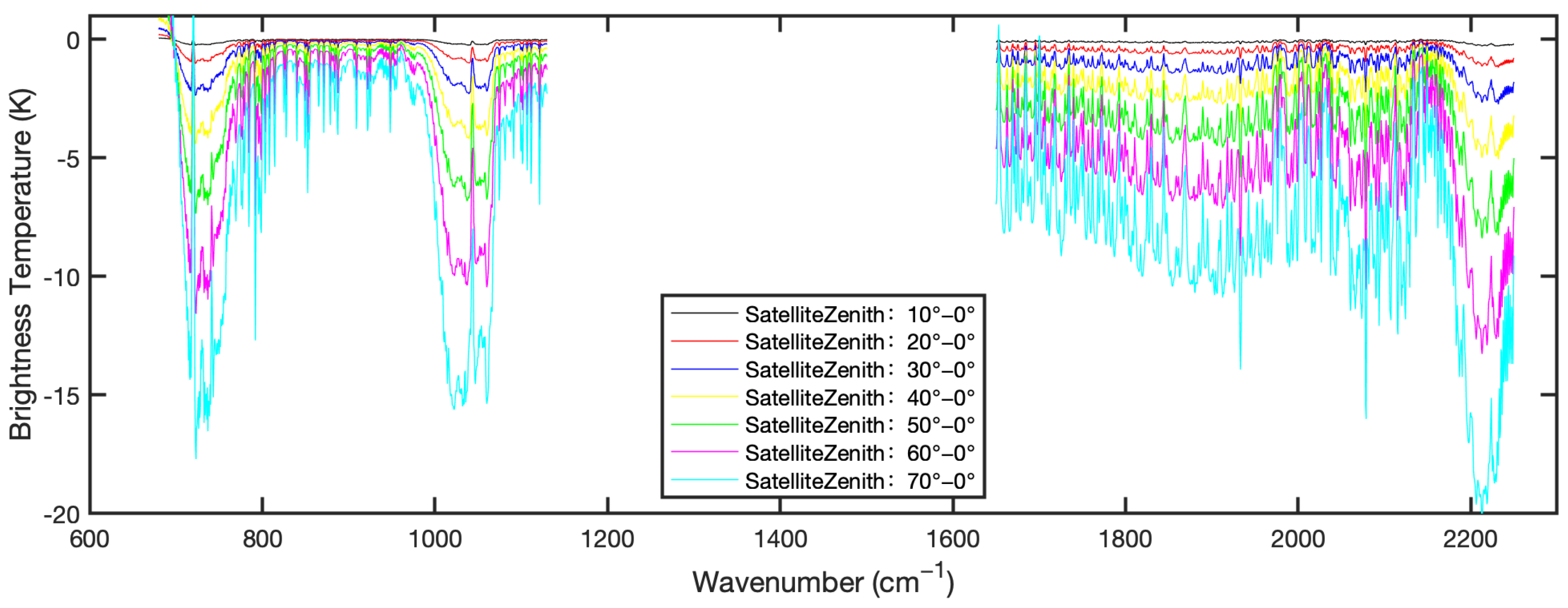
The observed fields of view on both sides of the nadir (satellite zenith = 0°) of a geostationary meteorological satellite have different degrees of deformation, and the deformation rate increases with increasing satellite zenith angle. The brightness temperature spectrum of GIIRS observations with different satellite zenith angles simulated from RTTOV using the U.S. Standard atmospheric profiles are shown in Figure 1. The different color lines represent the bias between the simulated brightness temperature with satellite zenith angles of 10°, 20°, 30°, 40°, 50°, 60°, and 70° minus the nadir simulation. The simulated brightness temperatures are very sensitive to the satellite zenith angle, especially the difference due to the change in satellite zenith angles in some absorption bands, which can be more than 10 K. The satellite zenith angles must be considered when retrieving the atmospheric temperature and humidity profiles. Eight sets of 1D-Net convolutional neural network retrieval models were built in this study by classifying the satellite zenith angles from 0° to 80° at 10° intervals.
When the actual observed satellite zenith angle is θ, the two nearest satellite zenith angles and classifications are found and the corresponding models to retrieve two sets of atmospheric profiles and are used, respectively. Then, the final retrieval parameters are obtained by linear interpolation as Equations (1)–(3):
3.2. Training Data for the Three-Dimensional Scheme U-Net 1
The training dataset for the three-dimensional (3D) atmospheric temperature and humidity profile retrieval consists of the two-dimensional (horizontal) real GIIRS brightness temperature observations covering the China area and the temporal-spatial matched horizontal atmospheric temperature and humidity fields from ERA5 reanalysis data. The sample can be viewed as picture data and is correlated and continuous in horizontal space.
The input data dimension of the U-Net convolutional neural network algorithm is [H(input) × W(input) × C1(input)], and the output data dimension is [H(output) × W(output) × C2(output)], where H and W are the length and width of the sample image, respectively. The input is the GIIRS observed 225 channels (C1) brightness temperature, and the output is the atmospheric parameter of 37 vertical pressure levels (C2).
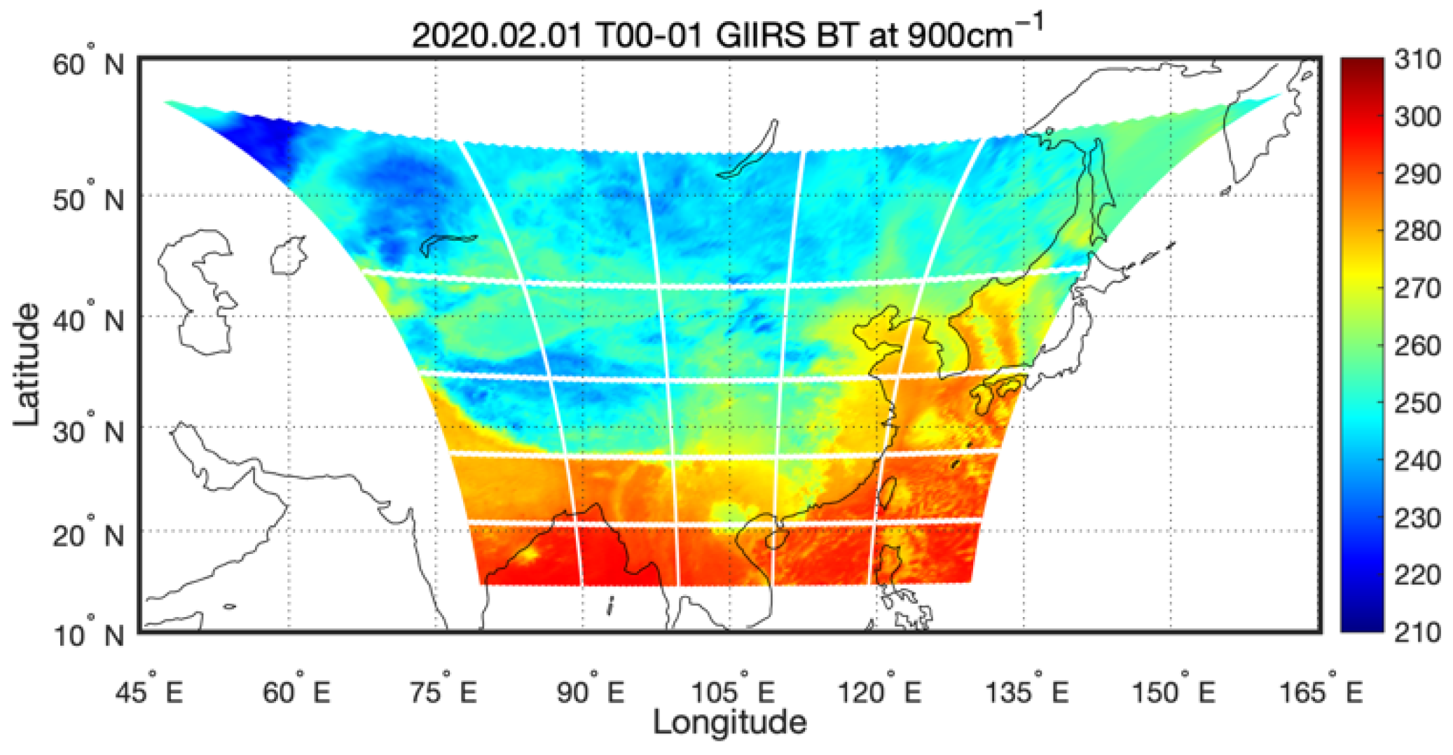
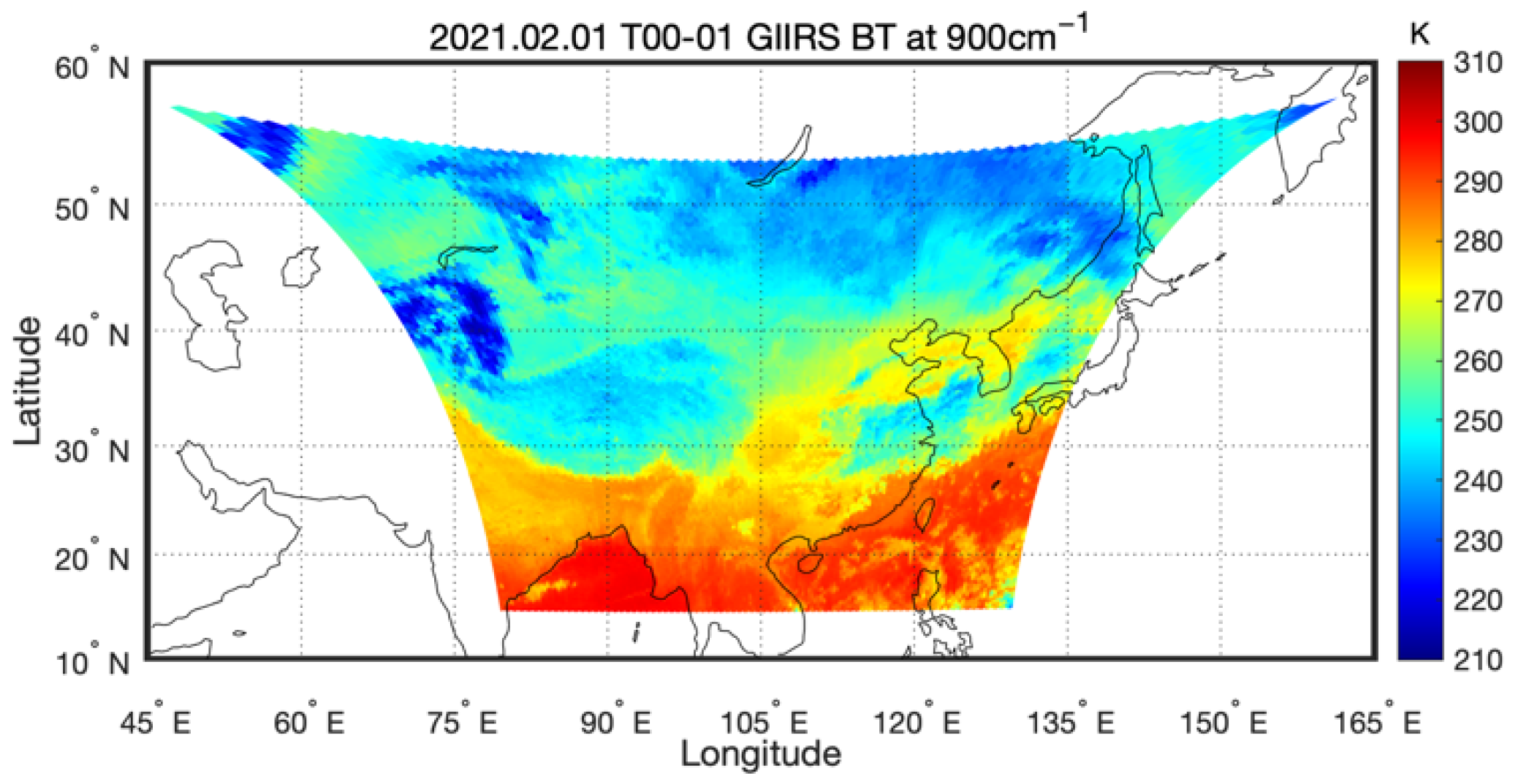
Each GIIRS observation FOR consists of 128 FOVs arranged in a 32 × 4 array. The U-Net 1 scheme spliced the observed brightness temperature of every eight consecutive FORs in the longitudinal direction to form a 32 × 32 pixel picture sample. Figure 2 shows the observed brightness temperature of the GIIRS 900 channel in China from 00 to 01 (UTC) on 01 February 2020. Each white box in Figure 2 represents a sample size including 32 × 32 FOVs, where the horizontal lines represent different scan belts. The ERA5 data were spatially interpolated to the 32 × 32 pixel image. A total of 4454 pairs of samples were matched from 01 February 2020 to 10 February 2020, as detailed in Table 2.
3.3. Training Data for the Three-Dimensional Scheme U-Net 2
The U-Net 2 scheme selected the continuous GIIRS observations of the whole China area as a sample image with 160 × 160 FOVs (the full coverage area in Figure 2). There are 284 training samples for the whole month of February 2020. The input data for the U-Net 2 model are 225 channel GIIRS observations with dimensions of [160 × 160 × 225], and the output data are atmospheric parameter retrievals of 37 pressure levels with dimensions of [160 × 160 × 37].
3.4. Model Structure and Parameter Optimization
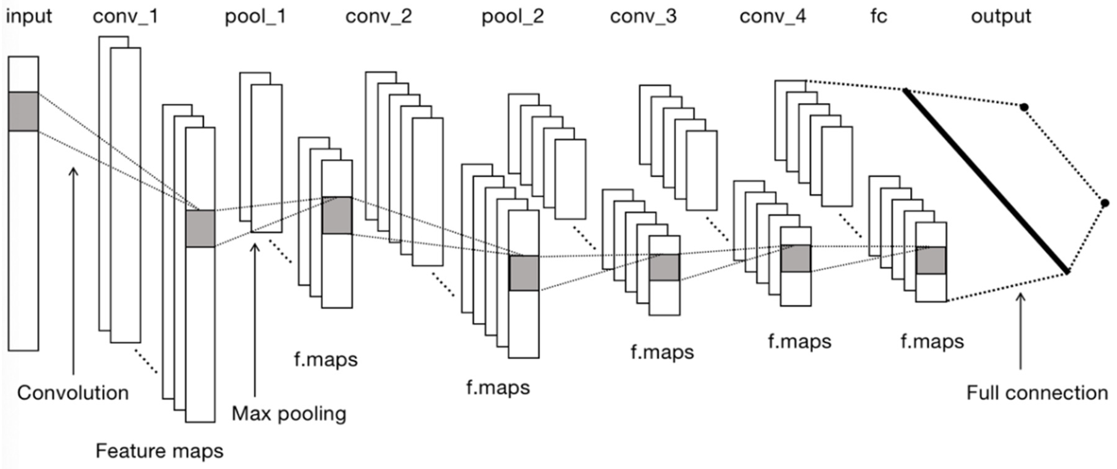
The structure of a traditional convolutional neural network mainly includes an input layer, convolutional layer, pooling layer, fully connected layer, and output layer. The main function of the convolutional layer is to extract features from the input image, the pooling layer is equivalent to a downsampling process, and the fully connected layer combines the local features extracted from the previous layers into the global features by nonlinear combination.
The 1D-Net model used in this study contains 1 input layer, 4 convolutional layers, 2 pooling layers, 1 fully connected layer, and 1 regression output layer. The convolutional layers and pooling layers are set alternately to form a multilayer neural network. The frame structure is shown in Figure 3. The input layer is the brightness temperature of 225 channels for each sample, which can be considered as a one-dimensional image of width 1, so the input layer size is 225 × 1. The output layer is the atmospheric temperature and humidity profiles with a size of 1 × 101. The dark part of the figure is the convolution kernel size, and the convolution operation is performed with a 1D convolution kernel. To build the optimal network, indicators such as retrieval root-mean-square error (RMSE), RMSE of network validation and network training time for test data are calculated for different parameter settings. The network optimal parameters were finally determined as follows: the convolution kernel size was 5 × 1, each pooling layer was 2 × 1 averaged pooling, the activation function was ReLU, and the training optimizer was Adam.
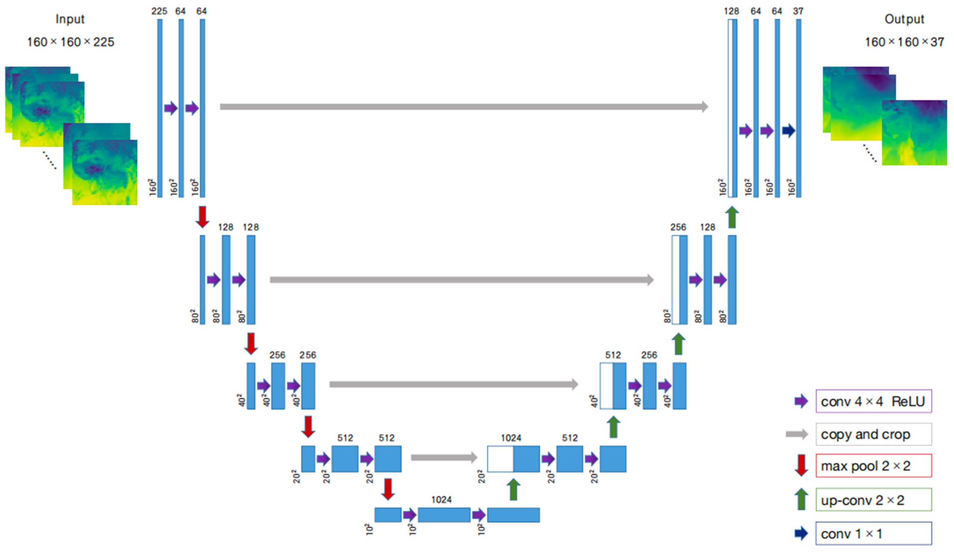
The U-Net convolutional neural network is a transformation of the traditional convolutional neural network and consists of two basic structure paths. The first is the contracting path, also called the encoder or analysis path, whose purpose is to capture the information in the image by convolution and pooling processes similar to the regular convolutional network. The second path is the expanding path, also known as the decoder or synthesizer path, which consists of upwards deconvolution and connecting features from the contracting path. Its purpose is to achieve precise localization of the segmented part of the image information and improve the output picture resolution. The structure of the U-Net 2 network constructed in this study is shown in Figure 4, with the contracting path on the left and the expanding path on the right. The purple arrows represent the convolution process (the convolution kernel size is 4 × 4), and each convolution process is followed by a modified linear unit called a ReLU. The grey arrows represent the crop and concatenation process, the red arrows represent the pooling process (2 × 2 maximum pooling method), and the green arrows represent the upconvolution process (2 × 2 convolution kernel). The number above the blue box indicates the number of channels in each layer, and the left box is the image size. The feature maps of the two parts are integrated using 4 crop and concatenation structures (grey arrows in Figure 4).
4. Validation of Retrieval Results
4.1. Comparison with ERA5 Reanalysis
GIIRS Level 2 operational products downloaded from the CMDC website include CLM, temperature profiles (available only for clear sky and above the cloud top for cloudy field of view), etc., but humidity products were not released.
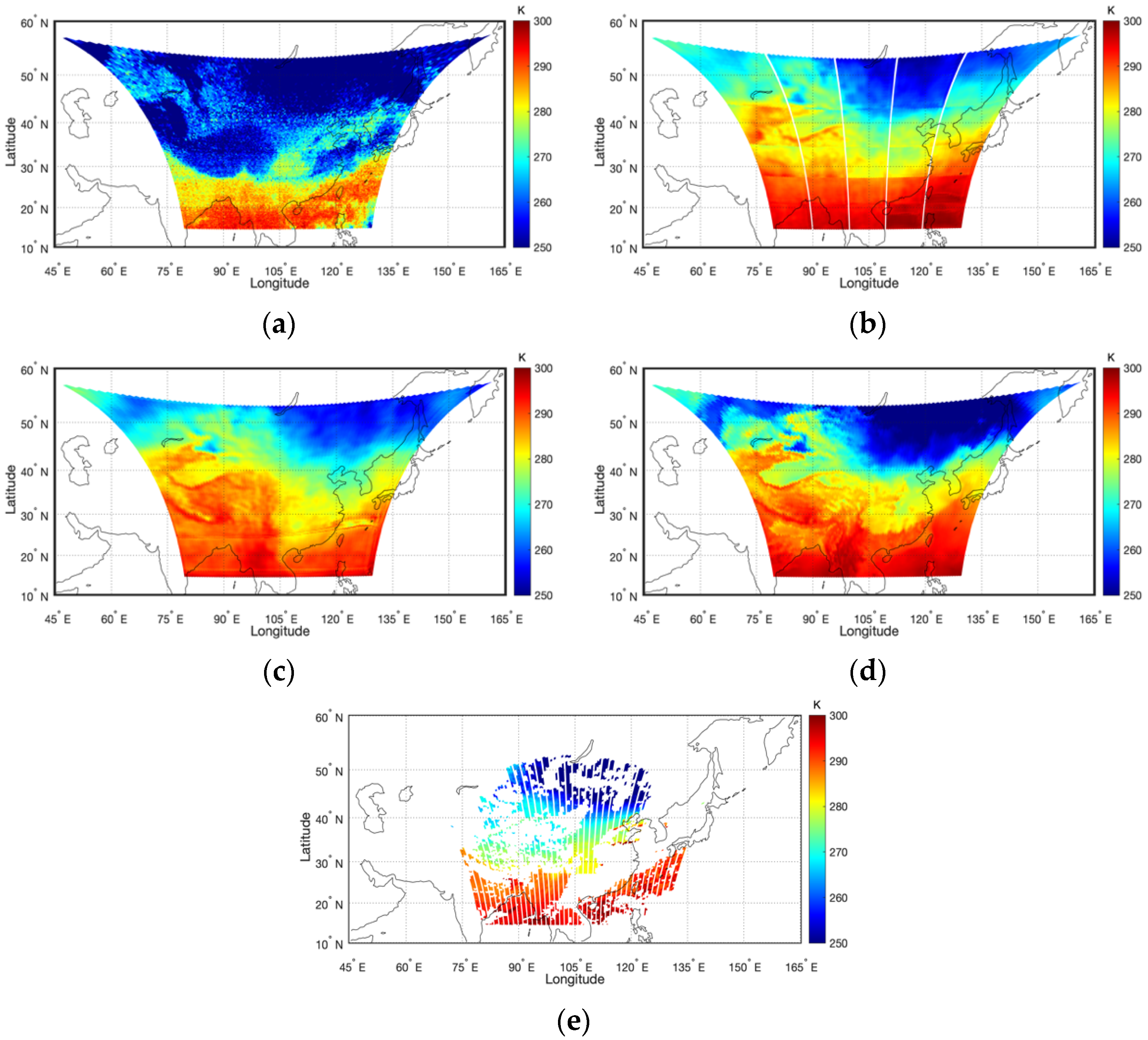
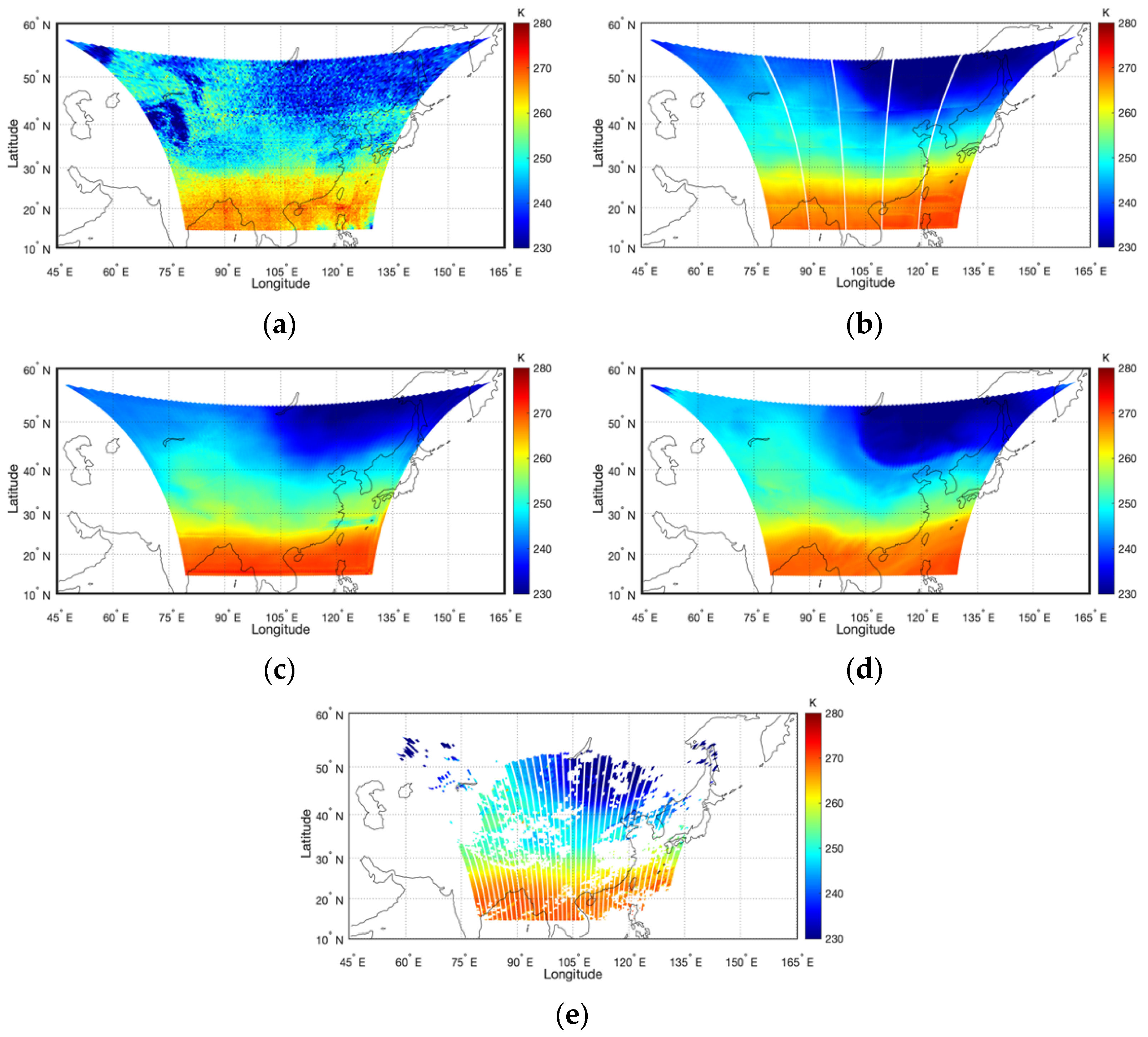
To test the retrieval accuracy of the above 1D-Net scheme and the two U-Net schemes, the temperature retrievals are compared with the ERA5 reanalysis fields and the GIIRS L2 operational atmospheric products. Using the GIIRS observation covering China at 00 to 01 (UTC) on 01 February 2021 as an example, the observed brightness temperature of the 900 channel is shown in Figure 5. The warm areas in the figure represent the clear sky area with relatively high brightness temperature, while the cool tone areas with low values are covered with clouds. The lower the brightness temperature is, the higher the vertical cloud development height. The temperature retrievals at 1000 hPa are shown in Figure 6, where (a) is the 1D-Net scheme, (b) is the U-Net 1 scheme, (c) is the U-Net 2 scheme, and (d) and (e) are the temperature fields of GIIRS L2 and ERA5, respectively. Figure 7 illustrates the temperature retrievals at 500 hPa. The blank pixels in Figure 6e correspond to the GIIRS L2 temperature lacking FOV, and an increasing number of FOVs are missing as the height decreases because no L2 temperature product is below the cloud top under cloudy conditions. The retrieved temperature fields both at 1000 hPa and 500 hPa from the two U-Net schemes and L2 operational products are all closer to the ERA5 reanalysis field in terms of horizontal spatial distribution and values, especially for the U-Net 2 scheme, while the 1D-Net scheme is slightly worse. At 1000 hPa, the retrieval from the 1D-Net scheme is generally low (especially at high latitudes) with a large difference from ERA5. The temperatures from the two U-Net schemes are higher than those from ERA5 in the region of [60°–75°E, 50°–55°N], GIIRS L2 temperatures are underestimated relative to ERA5, the U-Net 1 retrievals are also low, and the U-Net 2 retrievals are closest to the EAR5 reanalysis in the Tibetan Plateau. The retrieved field of various schemes at 500 hPa is closer to ERA5 than that at 1000 hPa, indicating that the high-level retrieval accuracy is higher than near the surface. Since the training sample of the U-Net 1 scheme is composed of segmented small region images, traces of the segmented areas can be clearly seen in the temperature retrievals, and the retrieved temperature fields are less continuous near the region boundary. The U-Net 2 training sample is the whole China area image, so the retrieved fields are very continuous in horizontal space and are closer to the ERA5 temperature fields.
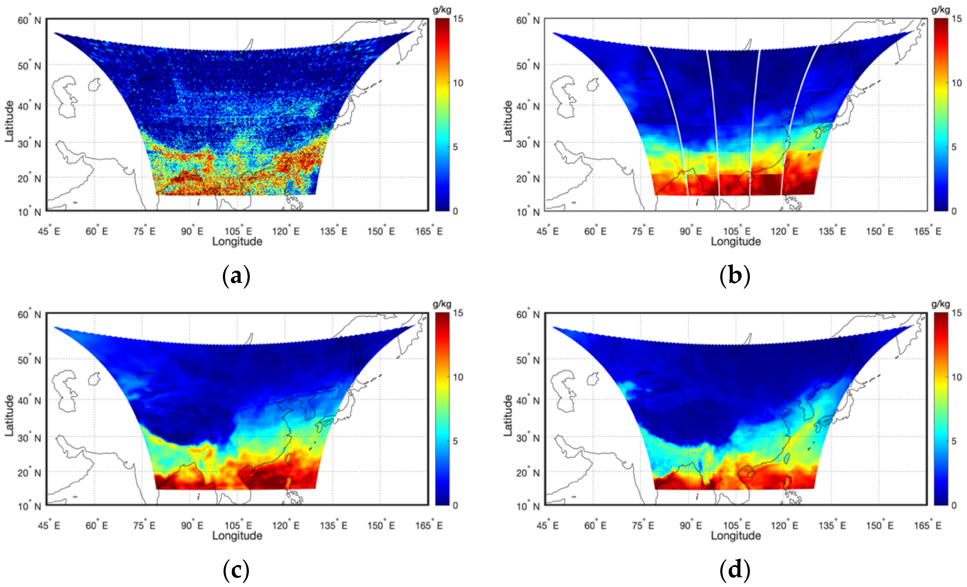
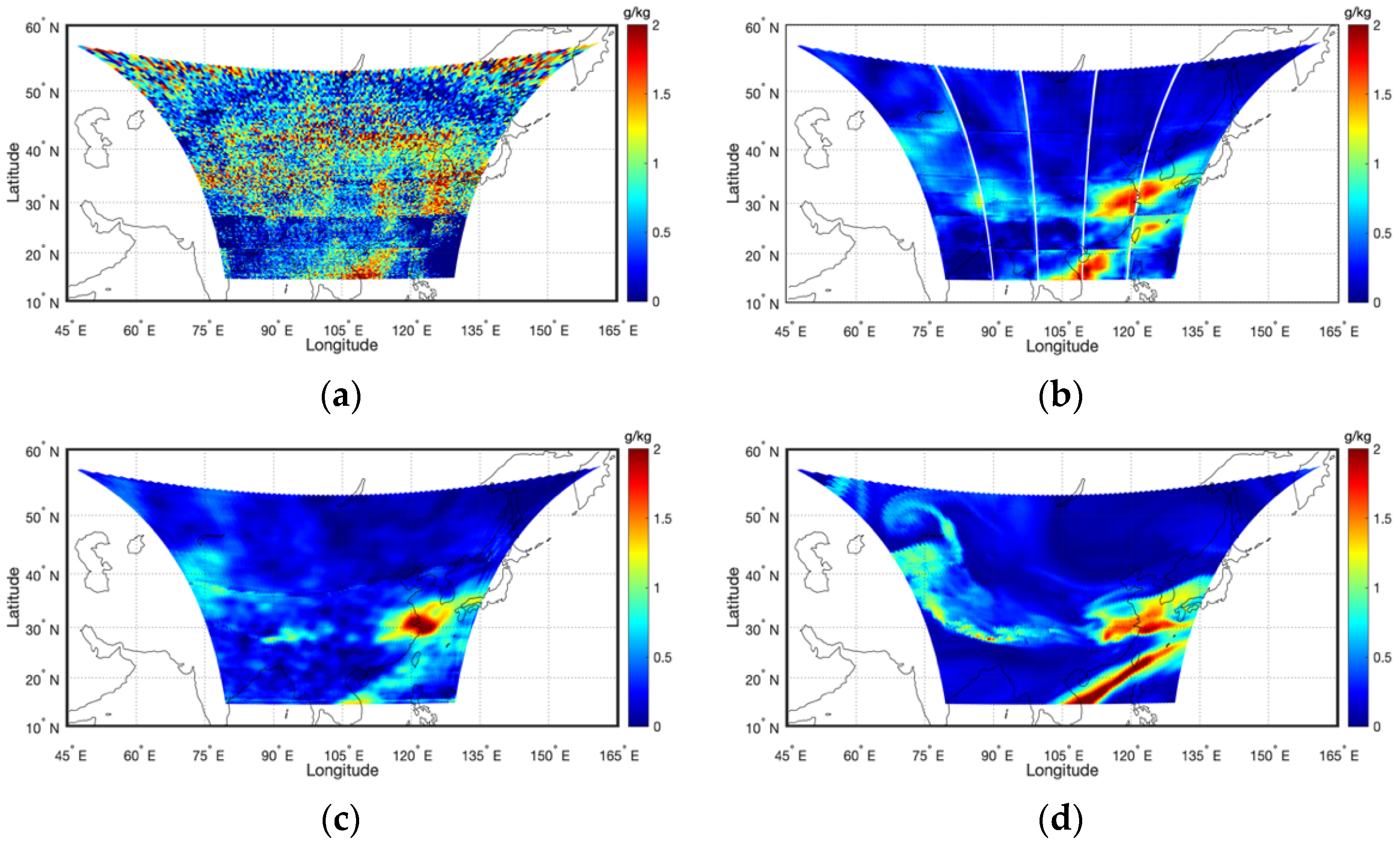
The humidity retrieved results are shown in Figure 8 (at 1000 hPa) and Figure 9 (at 500 hPa). (a), (b), and (c) give the retrievals of the 1D-Net scheme, U-Net 1 scheme, and U-Net 2 scheme, respectively, and (d) is from ERA5. Humidity profiles are not provided in the GIIRS L2 products. The large value area of warm colors indicates abundant water vapor, and the cold tone corresponds to the low value dry area. The retrieved humidity fields of the two U-Net schemes are relatively close to the ERA5 reanalysis at 1000 hPa and 500 hPa, while the difference is large for the 1D-Net scheme, especially at 500 hPa. There are many clutter points of 1D-Net because this scheme only carries out retrieval of the vertical dimension for each field of view independently. The two U-Net water vapor retrievals at 500 hPa have relatively high values on the northwest side of the Tibetan Plateau, which coincides with the lower brightness temperature in Figure 5. Low brightness temperature implies cloud cover and high water vapor content. The retrieved high value areas of water vapor correspond to the low brightness temperature in Figure 5, which indicates that the retrieved results are very effective. Similarly, traces of segmented small areas can be seen in the humidity from the U-Net 1 scheme.
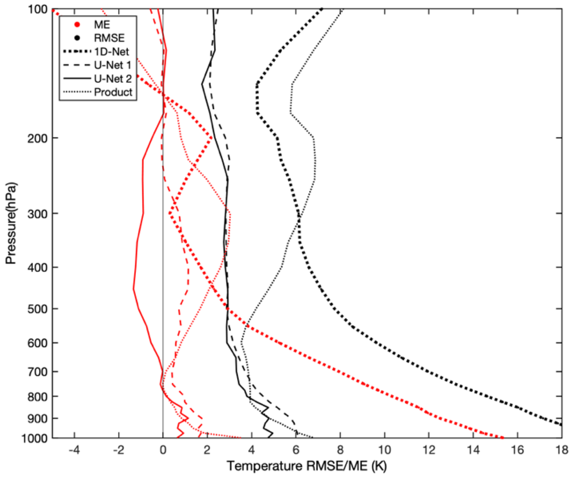
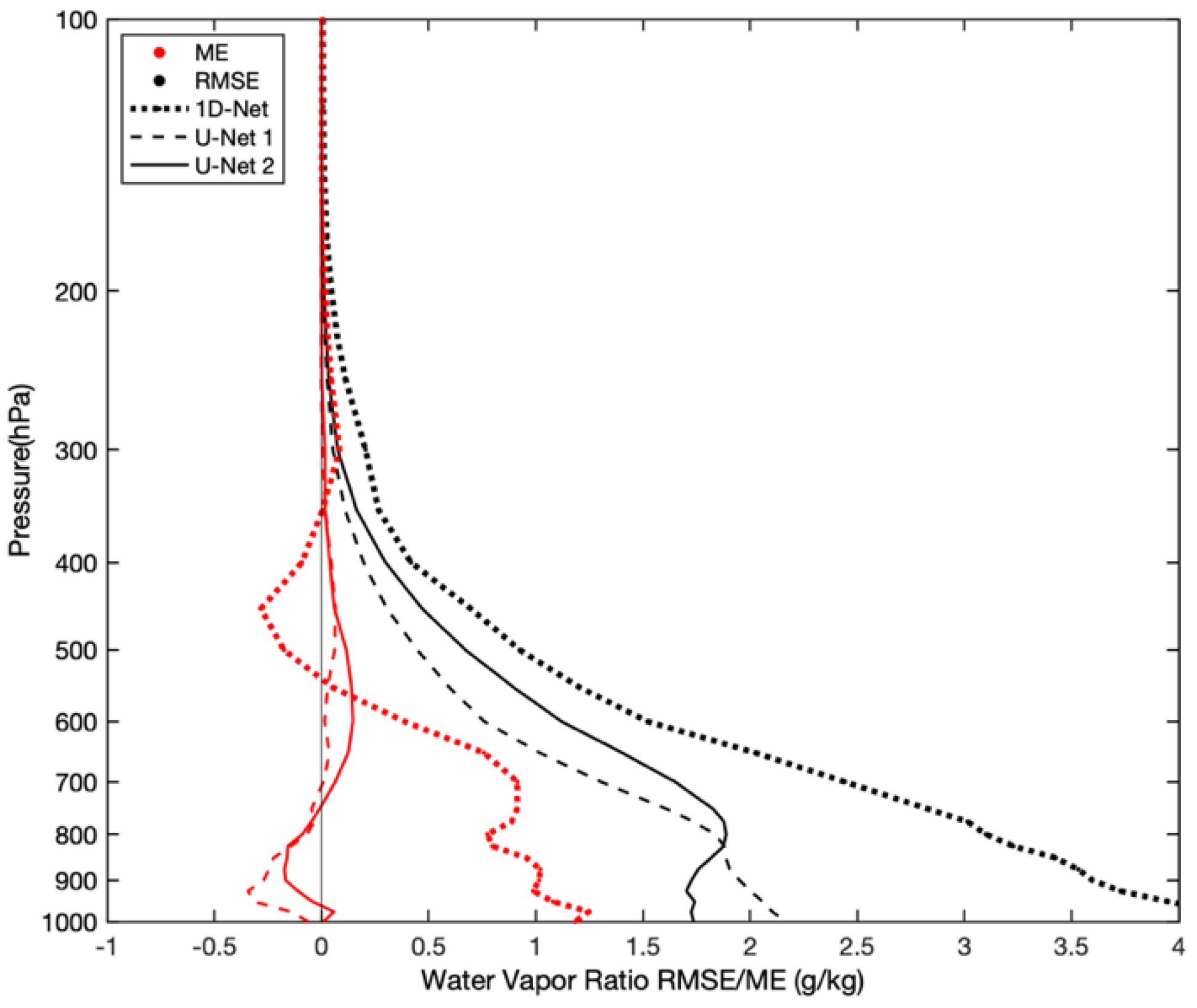
To quantitative test the retrieval accuracy, the temperature and humidity ME (mean error) and RMSE (root mean square error) profiles from the three schemes and GIIRS L2 products compared with ERA5 reanalysis data for the whole February 2021 are given in Figure 10 and Figure 11 respectively. The red lines are ME profiles, the black lines are RMSE profiles. The thicker dash-dotted line represents the 1D-Net scheme, the dashed line is the U-Net 1 scheme, the solid line is the U-Net 2 scheme, and the thinner dash-dotted line represents the L2 operational products. Figure 10 shows that most of the heights of these schemes are positive bias except for U-Net 2 from 750–150 hPa. The MEs of the two U-Net schemes are within 1 K at all pressure levels. The bias of 1D-Net scheme is significantly increased below 300 hPa. The RMSE of U-Net 1 and U-Net 2 are much smaller than 1D-Net. U-Net 2 scheme is better than that of the U-Net 1 scheme at all pressure levels. The accuracy of L2 products is close to two U-Net schemes below 700 hPa, but the RMSE increases with height. The retrieval error profiles of water vapor mixing ratio are shown in Figure 11. Humidity products are not provided by the L2 operational products. The humidity bias of two U-Net is close to 0 g/kg at all pressure levels, while 1D-Net scheme bias is larger than U-Net schemes. RMSE of all schemes decreases with height. The values of two U-Net schemes are smaller than 1D-Net. U-Net 1 humidity RMSE is lower than that of U-Net 2 above 800 hPa.
4.2. Comparison with Radiosonde Observations
The retrievals of the three schemes are evaluated in terms of mean error and root mean square error using temporal-spatial matched radiosonde observations as true. It is divided into all sky and clear sky for the retrieval accuracy check separately based on observations from the whole month data of February 2021. The determination of clear FOV was based on the GIIRS L2 operational CLM products, which made clear sky and cloud judgements for each FOV.
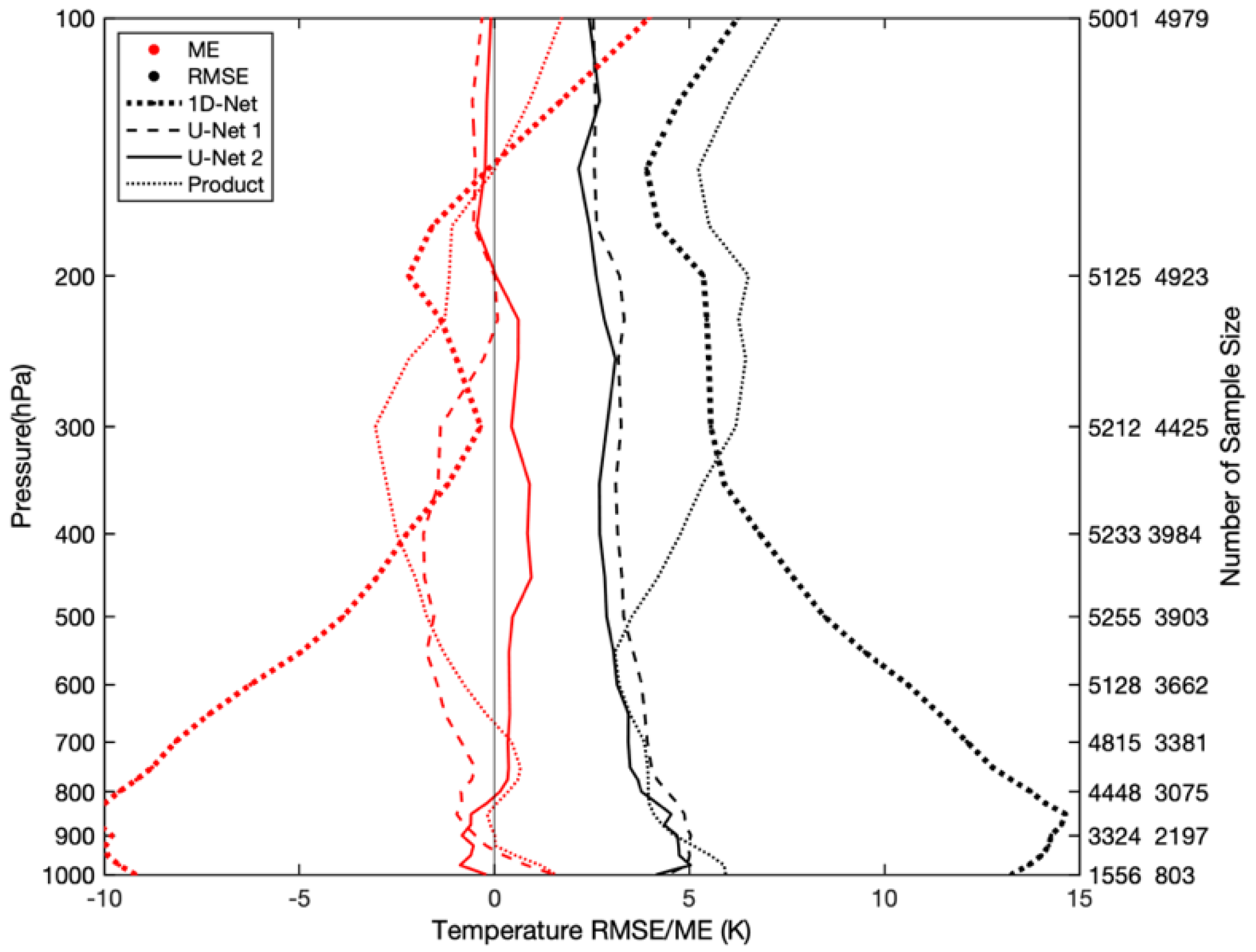
The bias profile of the temperature retrieval under clear sky conditions for February 2021 is shown in Figure 12. The color and line shape denote the same as Figure 10. The sample number used to calculate the MEs and RMSEs at each pressure level is given on the right vertical coordinate. The sample number matched in each level decreases with decreasing altitude, which is because some radiosonde stations have no data at very low altitudes affected by the terrain. Figure 12 shows that the RMSEs of these scheme retrievals all slightly decrease with increasing height under clear FOVs (except near the surface), and the accuracy of the L2 operational products is higher with RMSE within 3 K. The retrieval accuracy of the two U-Net schemes is similar to that of the L2 operational products in the upper troposphere. The 1D-Net scheme RMSE is significantly larger at all pressure levels, and the U-Net 2 RMSE is slightly smaller than that of U-Net 1. The MEs of the two U-Net schemes and L2 products are close to 0 K with high accuracy above 250 hPa. L2 operational products have the smallest bias above 500 hPa, and the biases of the two U-Net schemes are smaller at heights below 500 hPa.
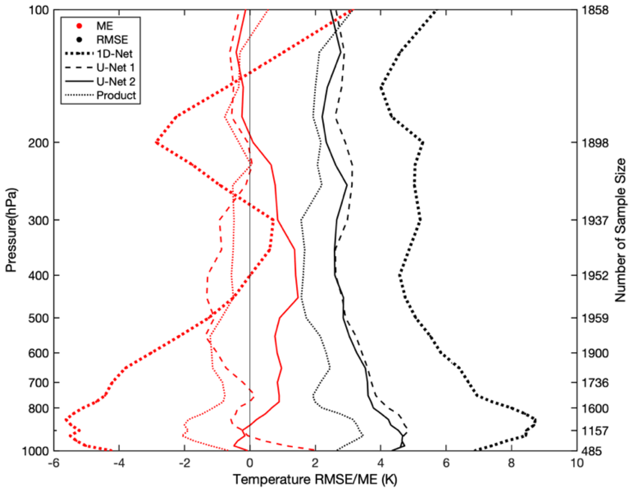
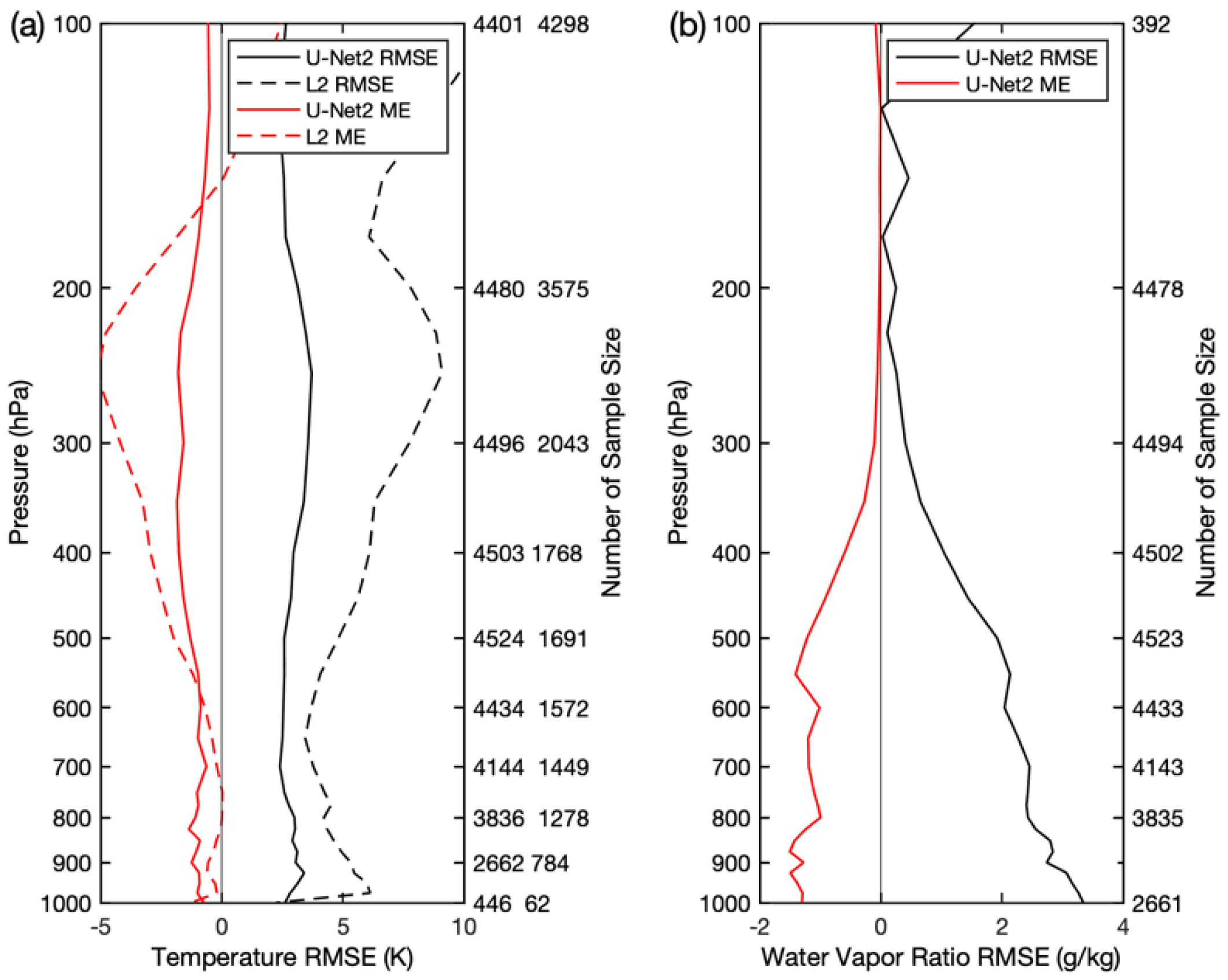
The bias profile of the temperature retrieval under all sky conditions for February 2021 is shown in Figure 13. The red lines are the ME profiles, the black lines are the RMSE profiles. The number in the first column of the right vertical coordinate of Figure 13 represents the statistical sample size of the three convolutional neural network schemes for each pressure level matched with radiosonde observations, and the second column one represents the sample number matched with GIIRS L2 operational products, which is less than that of the convolutional neural network scheme because GIIRS L2 operational products are not retrieved below the cloud top. The RMSEs of the temperature retrieval by the two U-Net schemes are lower than those of the L2 products at almost all levels in Figure 13, and the Level 2 RMSE increases substantially above 500 hPa. The RMSEs of the two U-Net schemes are relatively large near the surface, and the accuracy of temperature gradually increases slightly with altitude above 800 hPa, with an RMSE of approximately 2.5 K. The retrieval accuracy of the U-Net 2 scheme is approximately 0.5 K better than that of the U-Net 1 scheme at all pressure levels. In terms of the temperature ME, the U-Net 2 scheme has a positive bias above 800 hPa, while the L2 operational products and U-Net 1 scheme have a negative bias, especially the bias of the L2 products above 550 hPa, which is large with the gradually increasing RMSE. The U-Net 2 scheme bias is the smallest, with a value of approximately 0.5 K. The 1D-Net scheme has a large ME and RMSE below 400 hPa.
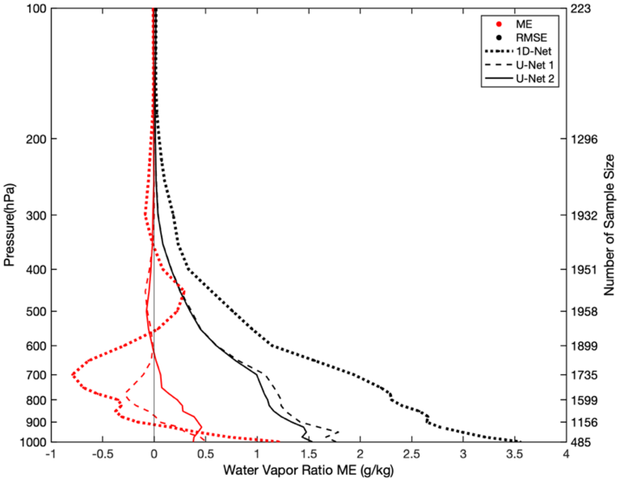
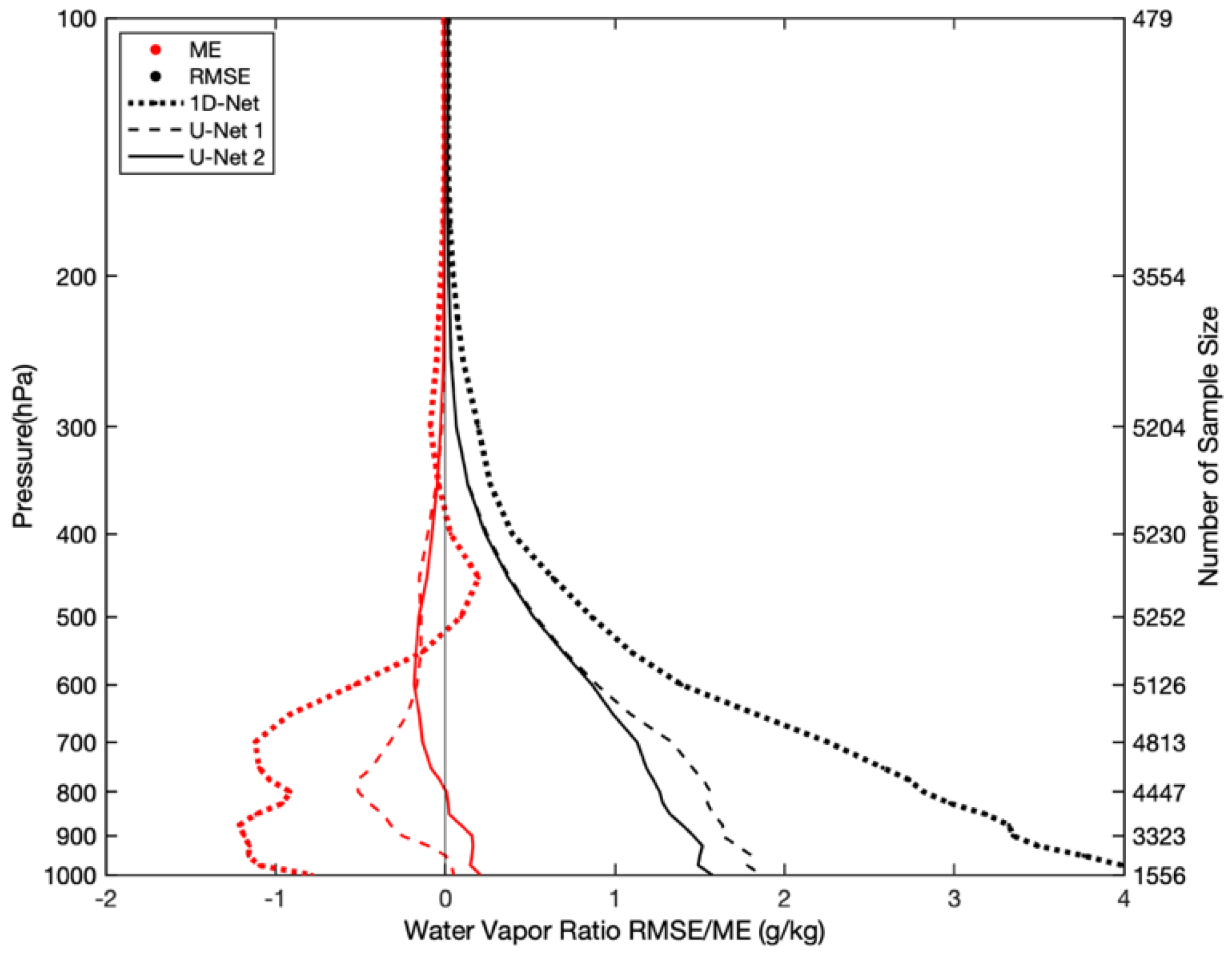
The ME and RMSE profiles of the retrieved humidity for all sky and clear sky FOVs for February 2021 are shown in Figure 14 and Figure 15, respectively. Again, the sample number used to calculate the error is given for each pressure level on the right vertical coordinate. Humidity products are not provided by the L2 operational products. It can be seen from the figures that the RMSEs decrease with increasing height in both all sky conditions and clear sky conditions. The RMSE is maximum for the 1D-Net scheme at all levels, and the U-Net 1 RMSE is slightly larger than that of U-Net 2 at altitudes below 650 hPa. The bias of the 1D-Net scheme is larger than that of the U-Net schemes for almost all altitudes, the MEs of the two U-Net schemes above 650 hPa are similar (both close to 0 g/kg), and the water vapor bias of U-Net 2 is relatively small below 650 hPa.
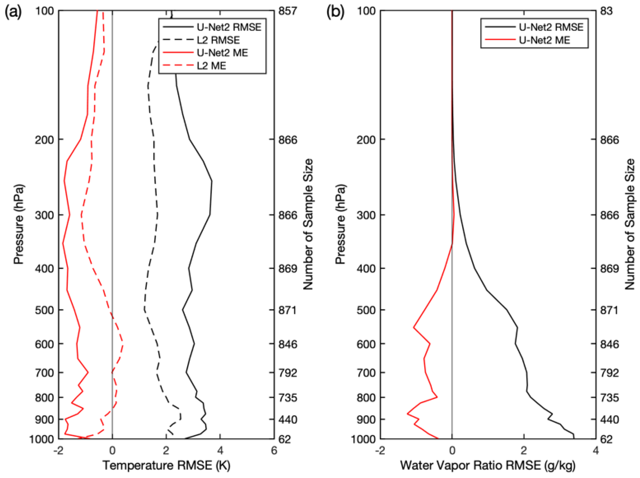
The GIIRS observations from July 2021 are used to further test the universality of these schemes. For summer months, the matched July 2020 data are trained to build network. The retrieval error of temperature and humidity under clear FOVs and all sky are shown in Figure 16 and Figure 17, respectively. The U-Net 2 algorithm gives the highest retrieval accuracy in above winter month, so we just compare the U-Net 2 with L2 products in July. The solid line is U-Net 2 scheme and dashed line represents the L2 operational products. In Figure 16a, the U-Net 2 temperature is negative bias in summer while positive ones in winter (Figure 12). To bias and RMSE, the L2 products accuracy are all better than U-Net 2 for clear FOVs. The summer RMSE of L2 products is smaller than winter. To humidity (Figure 16b), the positive bias of U-Net 2 in wither (Figure 13) also changes to negative bias. This means that U-Net 2 overestimates the temperature and humidity slightly in winter and underestimates it in summer. The summer humidity RMSE is bigger than winter.
Under all sky conditions (Figure 17), the temperature retrieval accuracy of U-Net 2 is obviously higher than L2 product no matter ME or RMSE in summer and the U-Net 2 improve the temperature retrieval in the middle and lower troposphere. The summer humidity retrieval is worse than in winter.
4.3. Discussion of Three Convolution Neural Network Schemes
The three deep learning convolutional neural network schemes all can retrieve atmospheric temperature and humidity profiles for all the sky. The 1D-Net scheme with large retrieval bias is mainly because of just considering single FOV observations in the retrieval and fail to incorporate spatial information and feature transformations. While U-Net schemes consider the relevance from the image perspective and establish directly the relationship between the input image and output image by extracting image features and using 3D convolution. So, the U-Net temperature and humidity retrievals are more accurate and closer to the actual atmosphere, especially the U-Net 2 scheme. At the same time the retrieval fields are more continuous in horizontal distribution.
5. Conclusions
Three convolutional neural network schemes are used to retrieve one-dimensional and three-dimensional atmospheric temperature and humidity profiles, respectively, based on FY4A/GIIRS observations in this paper. The retrieval accuracy of the three schemes was examined and validated using ERA5 reanalysis fields and radiosonde observations under all sky and clear sky fields of view. The results are as follows:
- (1)
- Compared with the ERA5 reanalysis field and the GIIRS L2 operational products, the retrieval accuracy of the 1D-Net scheme needs to be improved, and the three-dimensional atmospheric temperature and humidity field retrieved by the two U-Net schemes are closer to the ERA5 reanalysis field in both distribution and value; in particular, U-Net 2 retrieval is more continuous in horizontal space.
- (2)
- The accuracy of L2 operational temperature products is the highest, the temperature retrieval RMSE for the two U-Net schemes is the second highest, and the RMSE and ME of the 1D-Net scheme are all larger compared with temporal-spatial matched radiosonde observations when the GIIRS field of view is completely clear. The temperature RMSE and bias of the two U-Net schemes under all sky conditions are lower than those of GIIRS L2 above 800 hPa, especially for the U-Net 2 scheme. The accuracy of the Level 2 temperature product will be reduced under the influence of clouds. The humidity RMSEs of the two U-Net schemes are within 2 g/kg, the 1D-Net scheme is worse, and humidity products are not provided by the L2 operational product.
- (3)
- The three deep learning convolutional neural network schemes all can retrieve 3D atmospheric temperature and humidity profiles for all the sky from the perspective of the image. The 1D-Net scheme only carries out retrieval of the vertical dimension for each field of view independently, with larger bias and discrete retrievals. The U-Net schemes use GIIRS multichannel spatial observations as input to improve the retrieval accuracy with cloud influence, and the retrieval fields are more continuous in horizontal distribution and closer to the actual atmosphere. The U-Net 2 scheme has the highest retrieval accuracy, followed by U-Net 1. The retrieval speed of the two U-Net schemes is nearly the same, faster than that of 1D-Net. The time required to retrieve the China area covered by the GIIRS is approximately 2–3 times longer than that of the U-Net schemes.
Author Contributions
Conceptualization, L.G. and S.Y.; methodology, L.G. and S.Y.; software, S.Y.; validation, L.G. and S.Y.; formal analysis, L.G. and S.Y.; investigation, L.G. and S.Y.; resources, L.G.; data curation, S.Y.; writing—original draft preparation, L.G. and S.Y.; writing—review and editing, L.G. and S.Y.; supervision, L.G.; project administration, L.G. All authors have read and agreed to the published version of the manuscript.
Funding
This work was supported by the National Natural Science Foundation of China under Grant No. 41975028.
Acknowledgments
We would like to thank the NSMC (National Satellite Meteorological Center) and the CMDC (China Meteorological Data Service Center) for sharing FY4A/GIIRS and Radiosonde data. We also thank the editor and reviewers for the comments that helped improve our manuscript.
Conflicts of Interest
The authors declare no conflict of interest.
References
- Li, J.; Li, J.; Otkin, J.; Schmit, T.J.; Liu, C.Y. Warning Information in a Preconvection Environment from the Geostationary Advanced Infrared Sounding System-A Simulation Study Using the IHOP Case. J. Appl. Meteorol. Climatol. 2011, 50, 776–783. [Google Scholar] [CrossRef]
- Li, J.; Fang, Z. The development of satellite meteorology-Challenges and Opportunities. Mettir. Mon. 2012, 38, 129–146. [Google Scholar]
- Yang, J.; Zhang, Z.; Wei, C.; Lu, F.; Guo, Q. Introducing the New Generation of Chinese Geostationary Weather Satellites, Fengyun-4. Bull. Am. Meteorol. Soc. 2017, 98, 1637–1658. [Google Scholar] [CrossRef]
- Geng, X.W.; Min, J.Z.; Yang, C.; Wang, Y.B.; Xu, D.M. Analysis of FY-4A AGRI Radiance Data Bias Characteristics and a Correction Experiment. Chin. J. Atmos. Sci. 2020, 44, 679–694. [Google Scholar] [CrossRef]
- Jiang, D.M.; Dong, C.H.; Lu, W.S. Preliminary Study on the Capacity of High Spectral Resolution Infrared Atmospheric Sounding Instrument Using AIRS Measurements. J. Remote Sens. 2006, 10, 586–592. [Google Scholar]
- Guan, L. Retrieving Atmospheric Profiles from MODIS/AIRS Observations. I. Eigenvector Regression Algorithms. J. Nanjing Inst. Meteorol. 2006, 6, 756–761. [Google Scholar] [CrossRef]
- Liu, H.; Dong, C.H.; Zhang, W.J.; Zhang, P. Retrieval of clear air atmospheric temperature profiles using AIRS observation. Acta Meteorol. Sin. 2006, 66, 513–519. [Google Scholar]
- Smith, W.L.; Weisz, E.; Kireev, S.V.; Zhou, D.K.; Li, Z.; Borbas, E.E. Dual-Regression Retrieval Algorithm for Real-Time Processing of Satellite Ultraspectral Radiances. J. Appl. Meteorol. Climatol. 2012, 51, 1455–1476. [Google Scholar] [CrossRef]
- Zhu, L.; Bao, Y.; Petropoulos, G.P.; Zhang, P.; Lu, F.; Lu, Q.; Wu, Y.; Xu, D. Temperature and Humidity Profiles Retrieval in a Plain Area from Fengyun-3D/HIRAS Sensor Using a 1D-VAR Assimilation Scheme. Remote Sens. 2020, 12, 435. [Google Scholar] [CrossRef] [Green Version]
- Xue, Q.; Guan, L.; Shi, X. One-Dimensional Variational Retrieval of Temperature and Humidity Profiles from the FY4A GIIRS. Adv. Atmos. Sci. 2022, 39, 471–486. [Google Scholar] [CrossRef]
- Singh, D.; Bhatia, R.C. Study of Temperature and Moisture Profiles Retrieved from Microwave and Hyperspectral Infrared Sounder Data Over Indian Regions. Indian J. Radio Space Phys. 2006, 35, 286–292. [Google Scholar]
- Malmgren-Hansen, D.; Laparra, V.; Nielsen, A.A.; Camps-Valls, G. Statistical Retrieval of Atmospheric Profiles with Deep Convolutional Neural Networks. ISPRS J. Photogramm. Remote Sens. 2019, 158, 231–240. [Google Scholar] [CrossRef] [Green Version]
- Zhang, S.; Guo, Y.H.; Wang, J.J. The development of deep convolution neural network and its applications on computer vision. Chin. J. Comput. 2019, 42, 453–482. [Google Scholar]
- Paoletti, M.E.; Haut, J.M.; Plaza, J.; Plaza, A. A New Deep Convolutional Neural Network for Fast Hyperspectral Image Classification. ISPRS J. Photogramm. Remote Sens. 2018, 145, 120–147. [Google Scholar] [CrossRef]
- Khurana, L.; Chauhan, A.; Naved, M.; Singh, P. Speech Recognition with Deep Learning. J. Phys. Conf. Ser. 2021, 1854, 012047. [Google Scholar] [CrossRef]
- Tan, J.; Chen, B.; Wang, W.; Yu, W.; Dai, W. Evaluating Precipitable Water Vapor Products From Fengyun-4A Meteorological Satellite Using Radiosonde, GNSS, and ERA5 Data. IEEE Trans. Geosci. Remote Sens. 2022, 60, 4106512. [Google Scholar] [CrossRef]
- Xu, W.; Wang, W.; Wang, N.; Chen, B. A New Algorithm for Himawari-8 Aerosol Optical Depth Retrieval by Integrating Regional PM₂.₅ Concentrations. IEEE Trans. Geosci. Remote Sens. 2022, 60, 4106711. [Google Scholar] [CrossRef]
- Saunders, R.; Hocking, J.; Turner, E.; Rayer, P.; Rundle, D.; Brunel, P.; Vidot, J.; Rocquet, P.; Matricardi, M.; Geer, A.; et al. An Update on the RTTOV Fast Radiative Transfer Model (Currently at Version 12). Geosci. Model Dev. 2018, 11, 2717–2737. [Google Scholar] [CrossRef] [Green Version]
- Zhu, L.; Li, J.; Zhao, Y.; Gong, H.; Li, W. Retrieval of Volcanic Ash Height from Satellite-Based Infrared Measurements: VOLCANIC ASH HEIGHT RETRIEVAL. J. Geophys. Res. Atmos. 2017, 122, 5364–5379. [Google Scholar] [CrossRef]
- Yao, S.H.; Guan, L. Atmospheric temperature and humidity profile retrievals using machine learning algorithm based on satellite-based infrared hyperspectral observations. Infrared Laser Eng. 2022, 51, 20210707. [Google Scholar]
Figure 1.
The simulated brightness temperature bias between different satellite zenith angles and 0° (American standard atmosphere).
Figure 1.
The simulated brightness temperature bias between different satellite zenith angles and 0° (American standard atmosphere).

Figure 2.
Example of U-Net training sample size.

Figure 3.
Frame structure for the 1D-Net model.

Figure 4.
U-Net model structure.

Figure 5.
The GIIRS observed 900 brightness temperatures (unit: K) for the China area from 00 to 01 (UTC) on 01 February 2021.
Figure 5.
The GIIRS observed 900 brightness temperatures (unit: K) for the China area from 00 to 01 (UTC) on 01 February 2021.

Figure 6.
Temperature fields (unit: K) at 1000 hPa from 00 to 01 (UTC) on 01 February 2021: (a) 1D-Net; (b) U-Net 1; (c) U-Net 2; (d) ERA5; (e) Level 2 product.
Figure 6.
Temperature fields (unit: K) at 1000 hPa from 00 to 01 (UTC) on 01 February 2021: (a) 1D-Net; (b) U-Net 1; (c) U-Net 2; (d) ERA5; (e) Level 2 product.

Figure 7.
Same as Figure 6 except for 500 hPa: (a) 1D-Net; (b) U-Net 1; (c) U-Net 2; (d) ERA5; (e) Level 2 product.
Figure 7.
Same as Figure 6 except for 500 hPa: (a) 1D-Net; (b) U-Net 1; (c) U-Net 2; (d) ERA5; (e) Level 2 product.

Figure 8.
Water vapor mixing ratio (unit: g/kg) at 1000 hPa from 00 to 01 (UTC) on 01 February 2021: (a) 1D-Net; (b) U-Net 1; (c) U-Net 2; (d) ERA5.
Figure 8.
Water vapor mixing ratio (unit: g/kg) at 1000 hPa from 00 to 01 (UTC) on 01 February 2021: (a) 1D-Net; (b) U-Net 1; (c) U-Net 2; (d) ERA5.

Figure 9.
Same as Figure 8 except for 500 hPa: (a) 1D-Net; (b) U-Net 1; (c) U-Net 2; (d) ERA5.
Figure 9.
Same as Figure 8 except for 500 hPa: (a) 1D-Net; (b) U-Net 1; (c) U-Net 2; (d) ERA5.

Figure 10.
Temperature retrieval error profiles compared with ERA5 reanalysis field for the whole February 2021. The red lines are ME profiles, the black lines are RMSE profiles. The thicker dash-dotted line represents the 1D-Net scheme, the dashed line is the U-Net 1 scheme, the solid line is the U-Net 2 scheme, and the thinner dash-dotted line represents the L2 operational products.

Figure 11.
The same as Figure 10 except for water vapor mixing ratio.
Figure 11.
The same as Figure 10 except for water vapor mixing ratio.

Figure 12.
Temperature retrieval error profiles compared with radiosonde under clear FOVs for February 2021. The color and line shape denote the same as Figure 10.
Figure 12.
Temperature retrieval error profiles compared with radiosonde under clear FOVs for February 2021. The color and line shape denote the same as Figure 10.

Figure 13.
Same as Figure 12 except for all sky.
Figure 13.
Same as Figure 12 except for all sky.

Figure 14.
Water vapor mixing ratio retrieval error profiles compared with radiosonde under clear FOVs for February 2021. The color and line shape denote the same as Figure 10.
Figure 14.
Water vapor mixing ratio retrieval error profiles compared with radiosonde under clear FOVs for February 2021. The color and line shape denote the same as Figure 10.

Figure 15.
Same as Figure 14 except for all sky.
Figure 15.
Same as Figure 14 except for all sky.

Figure 16.
Temperature (a) and water vapor mixing ratio (b) retrieval error profiles compared with radiosonde under clear FOVs for July 2021. The red lines are ME profiles, the black lines are the RMSE profiles. The solid line is U-Net 2 scheme and dashed line represents the L2 operational products.

Figure 17.
Same as Figure 16 except for all sky: (a) temperature retrieval error profiles; (b) water vapor mixing ratio retrieval error profiles.
Figure 17.
Same as Figure 16 except for all sky: (a) temperature retrieval error profiles; (b) water vapor mixing ratio retrieval error profiles.


Table 1.
Specifications of FY4A/GIIRS.
| Parameter | Performance |
|---|---|
| Spectral bandwidth | Longwave: 700–1130 |
| Mid wave: 1650–2250 | |
| Spectral resolution | 0.625 |
| Spectral channels | Longwave: 689 |
| Mid wave: 961 | |
| Sensitivity | Longwave: 0.5–1.12 |
| Mid wave: 0.1–0.14 | |
| Spatial resolution | 16 km (the nadir) |
| Temporal resolution | 67 min (China area) |
| Spectral calibration accuracy | 10 ppm |
| Radiation calibration accuracy | 1.5 K |
Table 2.
Sample parameters for network training.
| Model | Input Dimensions | Training Sample Size | Training Sample Size | Retrieval Time |
|---|---|---|---|---|
| 1D-Net | 225 × 1 | 1 × 101 | 11,528 pixels | 8′9″ |
| U-Net 1 | 32 × 32 × 225 | 32 × 32 × 37 | 4454 images | 3′27″ |
| U-Net 2 | 160 × 160 × 225 | 160 × 160 × 37 | 284 images | 3′9″ |
Publisher’s Note: MDPI stays neutral with regard to jurisdictional claims in published maps and institutional affiliations. |
© 2022 by the authors. Licensee MDPI, Basel, Switzerland. This article is an open access article distributed under the terms and conditions of the Creative Commons Attribution (CC BY) license (https://creativecommons.org/licenses/by/4.0/).
Share and Cite
MDPI and ACS Style
Yao, S.; Guan, L. Comparison of Three Convolution Neural Network Schemes to Retrieve Temperature and Humidity Profiles from the FY4A GIIRS Observations. Remote Sens. 2022, 14, 5112. https://doi.org/10.3390/rs14205112
AMA Style
Yao S, Guan L. Comparison of Three Convolution Neural Network Schemes to Retrieve Temperature and Humidity Profiles from the FY4A GIIRS Observations. Remote Sensing. 2022; 14(20):5112. https://doi.org/10.3390/rs14205112
Chicago/Turabian StyleYao, Shuhan, and Li Guan. 2022. "Comparison of Three Convolution Neural Network Schemes to Retrieve Temperature and Humidity Profiles from the FY4A GIIRS Observations" Remote Sensing 14, no. 20: 5112. https://doi.org/10.3390/rs14205112
Note that from the first issue of 2016, this journal uses article numbers instead of page numbers. See further details here.