
Particulate Matter Concentrations over South Korea: Impact of Meteorology and Other Pollutants


1
Centre de Météorologie Radar, Météo-France, 31100 Toulouse, France
2
Korea Institute of Civil Engineering and Building Technology, Goyang-si 10223, Korea
3
Faculty of Engineering, Hokkaido University, N13 W8, Kita-ku, Sapporo 060-8628, Japan
*
Author to whom correspondence should be addressed.
Remote Sens. 2022, 14(19), 4849; https://doi.org/10.3390/rs14194849
Submission received: 18 August 2022
/
Revised: 22 September 2022
/
Accepted: 23 September 2022
/
Published: 28 September 2022
(This article belongs to the Section Atmospheric Remote Sensing)
Abstract
:Air pollution is a serious challenge in South Korea and worldwide, and negatively impacts human health and mortality rates. To assess air quality and the spatiotemporal characteristics of atmospheric particulate matter (PM), PM concentrations were compared with meteorological conditions and the concentrations of other airborne pollutants over South Korea from 2015 to 2020, using different linear and non-linear models such as linear regression, generalized additive, and multivariable linear regression models. The results showed that meteorological conditions played a significant role in the formation, transportation, and deposition of air pollutants. PM2.5 levels peaked in January, while PM10 levels peaked in April. Both were at their lowest levels in July. Further, PM2.5 was the highest during winter, followed by spring, autumn, and summer, whereas PM10 was the highest in spring followed by winter, autumn, and summer. PM concentrations were negatively correlated with temperature, relative humidity, and precipitation. Wind speed had an inverse relationship with air quality; zonal and vertical wind components were positively and negatively correlated with PM, respectively. Furthermore, CO, black carbon, SO2, and SO4 had a positive relationship with PM. The impact of transboundary air pollution on PM concentration in South Korea was also elucidated using air mass trajectories.
1. Introduction
Poor air quality due to air pollution critically impacts human health and can lead to increased mortality rates as well as negative impacts on biodiversity, ecosystems, and regional climate [1]. Atmospheric particulate matter (PM) is a mixture of suspended liquid and solid particles that plays a significant role in air pollution. In recent decades, rapid industrialization and urbanization in East Asia have resulted in severe air pollution and frequent haze events in the region [2]. South Korea is a recently developed East Asian country located downwind of China, Mongolia, and Russia. Elevated PM concentrations occur in South Korea due to emissions from local traffic, industrial facilities, and the long-range transport of anthropogenic emissions, Asian dust, and wildfire ash [3]. PM concentrations vary depending on human activities, topography, and meteorological factors [4]. In particular, meteorological parameters play a significant role in the dispersion, transformation, and removal of air pollutants from the atmosphere [5]. Consequently, a regional meteorology analysis is required to fully describe the characteristics of PM [6].
Many studies have been conducted around the world to examine the physical and chemical properties of atmospheric PM, as well as the relationship between PM and meteorological parameters [6,7,8,9,10,11]. PM concentrations were negatively correlated with wind speed (WS), precipitation, and humidity, and positively correlated with pressure over China [12]. Furthermore, it is known that PM concentrations vary seasonally. Li et al. [13] found high PM2.5 and PM10 concentrations in winter and autumn and low concentrations in spring and summer in Shenyang, Northeastern China. Caramagna et al. [14] observed that fine particle concentrations (PM2.5 and PM10) were higher during working (high traffic) days and lower during non-working days over Catania (Italy). Brusca et al. [15] described the plume’s characteristics and the relationship between the plume and obstacles of various shapes using laboratory experiments.
Several researchers have investigated the variability of PM concentrations in South Korea. Kim et al. [3] observed that the inter-annual PM concentration was negatively correlated with WS variations over the Seoul metropolitan area. Furthermore, PM10 levels peaked in the spring and were positively correlated with SO2, NO2, and CO [11]. The Korea–United States Air Quality (KORUS-AQ) field campaign was conducted in South Korea from May–June 2016. This field campaign investigated the factors controlling air quality over the South Korean region using observations from three aircraft, an extensive ground-based network, and three ships as well as an array of air quality forecast models [16,17]. The campaign showed that the PM2.5 concentrations were higher over central Seoul than in coastal regions during transboundary transport days, due to gaseous urban emissions [18]. The transboundary pollution from China was mixed with the local pollution, and the heterogeneous chemical reactions produced high PM2.5 concentrations [19]. Foreign and domestic contributions have different effects on PM concentration in South Korea. Kumar et al. [20] investigated the contributions of foreign pollution (particularly from China) to PM2.5 levels in South Korea. They found that the Chinese anthropogenic contributions were greatest during the winter and spring seasons. The highest contribution was around 60% in January and February, and the lowest was in August. China accounted for 45% of annual anthropogenic emissions. They also stated that domestic contributions were lower than Chinese contributions both monthly and annually, and contributions from the rest of the world were minor. Xie and Liao [21] examined the effects of changes in anthropogenic emissions in China on PM2.5 concentrations in South Korea and Japan. The reduction in anthropogenic emissions in China resulted in a 7.7% and 7.9% decrease in PM2.5 concentrations in South Korea and Japan, respectively. Additionally, the reduction in anthropogenic emissions in China reduced the concentrations of sulfate, ammonium, BC, and OC in Korea and Japan. During the KORUS-AQ campaign, which was conducted from May 1 to June 12, 2016, Lee et al. [22] examined the impact of long-distance transboundary transport on the Korean peninsula. They concluded that anthropogenic emissions in East-Central China, particularly in the Shandong region, have a significant impact on aerosol pollution in the Korean region. Yim et al. [23] described the impact of local and transboundary air pollution on air quality in Japan and South Korea. According to the authors, local emissions in both Japan and Korea accounted for 30% of the pollution, while transboundary emissions, specifically emissions from China’s industrial sectors, accounted for the remaining 70%. Transboundary air pollution increased during favorable weather conditions (westerly or northwesterly winds) in the spring and winter seasons. Choi et al. [24] explored the effects of local and transboundary air pollution on PM2.5 concentrations in Korea during the months of May and June of 2016. During the extreme pollution period, the Chinese contribution was 68% and the local contribution was 26%. Chinese and domestic contributions were 25% and 57%, respectively, during the blocking period. Furthermore, they discussed the role of emission sources in pollution reduction: the most prominent were domestic anthropogenic NH3 emissions, followed by anthropogenic SO2 emissions from Shandong, domestic anthropogenic NOX, anthropogenic NH3 emissions from the Shandong region, domestic anthropogenic OC emissions, and domestic anthropogenic BC emissions. Park [25] observed a link between particulate matter concentration and mortality rate in Seoul, Korea. The author found that PM, NO2, and O3 concentrations were high during the winter and spring, resulting in a high probability of mortality. Deaths were unlikely in areas with low levels of PM, NO2, and O3. Pollutants have a significant impact on human health during extreme weather events (cold and heat waves). Han et al. [26] discovered high PM concentrations in the western and northwestern areas of the Seoul metropolitan region during winter haze events. The pollution is primarily attributed to foreign pollution (particularly Chinese emissions), but local pollution also plays an important role under high pressure with weak vertical mixing. Using clustering analysis, Lee et al. [27] identified the source regions for high PM10 concentrations in the Seoul region. High PM10 concentrations in Seoul were caused by external sources such as the Gobi desert area and major cities and industrial districts in inland China, as well as internal sources such as the Yellow Sea and inland Korea. According to Lee et al. [28], meteorological conditions such as atmospheric pressure distribution, air current movement, and atmospheric stability change can all play important roles in the occurrence and persistence of high-concentration air pollution episodes in the Korea region. The majority of the pollution transported from the Eastern China region is transported under favorable westerly conditions.
In recent years, South Korea has experienced significant industrial and economic growth, resulting in frequent and severe haze events and increased mortality associated with pollution. Despite the government’s efforts to control air pollution, poor air quality remains a serious issue. The KORUS-AQ field study examined the impact of meteorology on the relative influence of local and transboundary pollution and described the causes of poor air quality in South Korea. However, the KORUS-AQ study was conducted for only a short period of time during the spring, from 1 May to 10 June 2016. Thus, these studies were narrowly focused on a specific time period and were less concerned with the impact of various meteorological parameters on PM2.5 and PM10. Thus, the present study more comprehensively discusses the PM2.5 and PM10 characteristics across South Korea over a long period (2015–2020) and supports the findings of previous studies in this region. Furthermore, the monthly, seasonal, and annual distributions of PM were described, as well as the impact of various meteorological parameters, including the influence of local and foreign pollution at different time scales. We investigated the relationship between PM concentrations (both PM2.5 and PM10), other air pollutants (CO, black carbon (BC), SO2, SO4, and O3), and various meteorological parameters (temperature (T), specific humidity (QLML), WS, pressure (P), precipitation, wind direction, heat flux, and ground heating) for different time scales. To achieve this, we used various techniques and tools such as the Spearman correlation, generalized additive model (GAM), and multivariable linear regression model (MLR). Further, we used Hysplit model outputs to define and interpret the impact of transboundary pollution on the Korean peninsula.
2. Materials and Methods
Since the 1960s, the East Asian region has experienced rapid industrialization, urbanization, and economic growth [29], resulting in increased air pollution in all East Asian countries, including South Korea. To measure and monitor air pollution, the Korean government established the Korean Ministry of Environment (KMOE) Network in 1973, which is controlled by national and local government bodies. The network stations monitor various types of pollution (air quality), including city air quality, road-side air quality, acid deposition, background density, suburban air quality, heavy metals, harmful materials, photochemical pollutants, the global atmosphere, PM concentrations, and air pollution concentrations [30].
Figure 1 depicts South Korea’s 16 administrative areas, which include nine provinces and seven major cities. The KMOE conducts continuous automatic monitoring of PM concentrations in all 16 administrative areas using various monitoring equipment. We used KMOE data to investigate the relationship between PM concentration and meteorology in Korea. The KMOE network provides six different types of air pollutants, including PM10, PM2.5, O3, CO, SO2, and NO. The air pollution-related information and data are available at www.airkorea.or.kr (accessed on 8 July 2021). The network maintains data accuracy and quality and filters out abnormal data in four stages. Abnormal data are identified based on the conditions of the (1) measuring equipment (e.g., fault connection, malfunction, calibration) and if the data exceeds the normal range or rate of change, (2) if the data acquisition rate is less than 75%, (3) if there are large fluctuations in the data, and (4) if the data are inconsistent; and then the abnormal data filters automatically using inbuilt algorithms [31]. The accuracy of the data has been verified and used by several researchers for various air quality studies [3,11]. We also compared KMOE data with MERRA re-analysis datasets and found good agreement (figure not shown).
In the present study, we used PM2.5 and PM10 measurements from 220 monitoring stations across all administrative areas for six years (2015–2020). Monthly PM2.5 and PM10 data were converted into seasonal, inter-annual, and annual time scales for the 16 administrative areas and for the entire country. We used various meteorological parameters (T, QLML, precipitation, WS, horizontal (zonal U) and vertical (W) wind vectors, ground heating, pressure, and latent and sensible heat fluxes); the surface concentrations of pollutants including CO, BC, SO4, and SO2; aerosol optical depth (AOD); and the mass mixing ratio of O3 to explore their relationships with PM. Meteorological and pollutant parameters were collected from the state-of-the-art MERRA-2 reanalysis dataset for South Korea. Kim et al. [32] validated MERRA-2 data for the Korean Peninsula and found that it outperformed other reanalysis datasets. Several researchers have also used MERRA-2 data in different studies [33,34]. MERRA-2 data were developed and generated by the global modeling and assimilation office (GMAO) of the National Aeronautics and Space Administration (NASA) using the Goddard Earth observing system, version 5.12.4 data assimilation system [35]. MERRA-2 provides data at a 0.5° × 0.625° (latitude × longitude) spatial resolution and various temporal resolutions (one hourly minimum time step). In this study, monthly data were used to evaluate seasonal, inter-annual, and annual values for meteorological and pollutant parameters. In addition, the data for each province and the entire country were averaged.
2.1. Generalized Additive Model (GAM)
Simple linear regression models are frequently used in statistical applications. However, linear models often fail to accurately fit non-parametric or non-linear parameters [36]. GAMs are more advantageous for non-parametric applications because they can describe and interpret non-linear parameters due to their additive effects. GAM supports a wide range of distributions and link functions, which reduces the error in predicting the dependent variable. GAMs are effective at handling complex non-linearity in air pollution research and have been widely used to detect the relationship between air pollutants and meteorological parameters [36,37,38,39,40,41]. GAMs are regression models that use smoothing splines for covariates rather than parametric or linear coefficients [36,42]. The additive model in the context of time series concentration can be described as [42].
where yi is the ith air pollution concentration, β0 is the overall mean of the response, sj(xij) is the smooth function of the ith value of covariate j, n is the total number of covariates, εi is the ith residual, and var(ε) = σ2, which is assumed to be normally distributed. We used GAM to analyze the relationship between PM and meteorological parameters and other pollutants. The Akaike Information Criterion (AIC) and adjusted R2 were used to select the degrees of freedom, air pollutants, and the appropriate meteorological parameters [43]. The smoothing parameters were selected based on the restricted maximum likelihood (REML) method. The proposed adjusted model in the present study is as follows:
where PMk represents either PM2.5 or PM10. The meteorological parameters, pollutants, and PM were selected based on the smallest AIC and the largest adjusted R2, and cubic regression spline smoothing functions were used for meteorological factors, which were determined based on the REML standard All analyses were carried out in R using the “mgcv” package [44].
2.2. MLR Model
MLR model was used to delineate the relationships between multiple independent meteorological variables and a single dependent variable (pollutants). The MLR model was computed based on the ordinary least squares (OLS) method. The model is as follows:
where i represents the site locations in Korea; β0, β1, β2, β3, β4, β5 are the regression coefficients; y is the concentration of the independent pollutant variable; x is the meteorological variables (x1, x2, x3, x4, and x5 are the QLML, P, WS, T, and precipitation, respectively); and ε is the stochastic error associated with the regression.
2.3. HYSPLIT Model
The National Oceanic and Atmospheric Administration (NOAA) developed the hybrid single-particle Lagrangian Integrated Trajectory (HYSPLIT) to determine the transport paths of air masses. This model has been widely used to investigate the transport of air pollutants using forward- and back-trajectories. The model simulates air parcel trajectories, emission, difficult transport, deposition, dispersion, and chemical transformation. The NOAA’s global data assimilation system (GDAS) 1° × 1° grid resolution data were used to examine transboundary air pollution. For trajectory calculation, the model employs the NCEP/NCAR re-analysis meteorological dataset. Air mass trajectories define the transportation of aerosols from one location to other [45]. At specific weather conditions, the air mass carries a high number of aerosols and pollutants, which illustrates the heavy pollution or haze events. In the present study, we used 24 h back-trajectories during haze and non-haze events. The air mass backward trajectories were effective in determining the source of the pollution and its pathway to the receptor (long-range transportation) [45].
3. Results
3.1. Monthly Distribution of PM and Other Pollutants
Figure 2a,b show the monthly mean variability of PM2.5 and PM10 over South Korea from 2015 to 2020, respectively. There is a clear V-shaped distribution for both PM2.5 and PM10 throughout each year. PM2.5 concentrations were highest in December, January, and February, and lowest in July and August. In contrast, PM10 concentrations were highest in March and April and lowest in July and August. PM2.5 concentrations ranged from 10–40 μg m−3 and were higher than the World Health Organization (WHO) standard of 25 μg m−3. PM10 concentrations ranged at 20–80 μg m−3 and also exceeded the WHO recommended levels of 50 μg m−3. High PM concentrations were caused by industrial emissions and dust transport from neighboring countries in conjunction with favorable meteorological conditions [3]. The peak PM2.5 concentration (40 μg m−3) was observed in 2019, due to heavy haze events. Generally, both PM2.5 and PM10 tended to decrease over the study period, with the lowest PM concentrations observed in 2020 attributed to the full and partial lockdowns in China and Korea to prevent the spread of the novel coronavirus (COVID-19). During this period, major industries were closed, and traffic significantly decreased, which had a considerable impact on emissions.
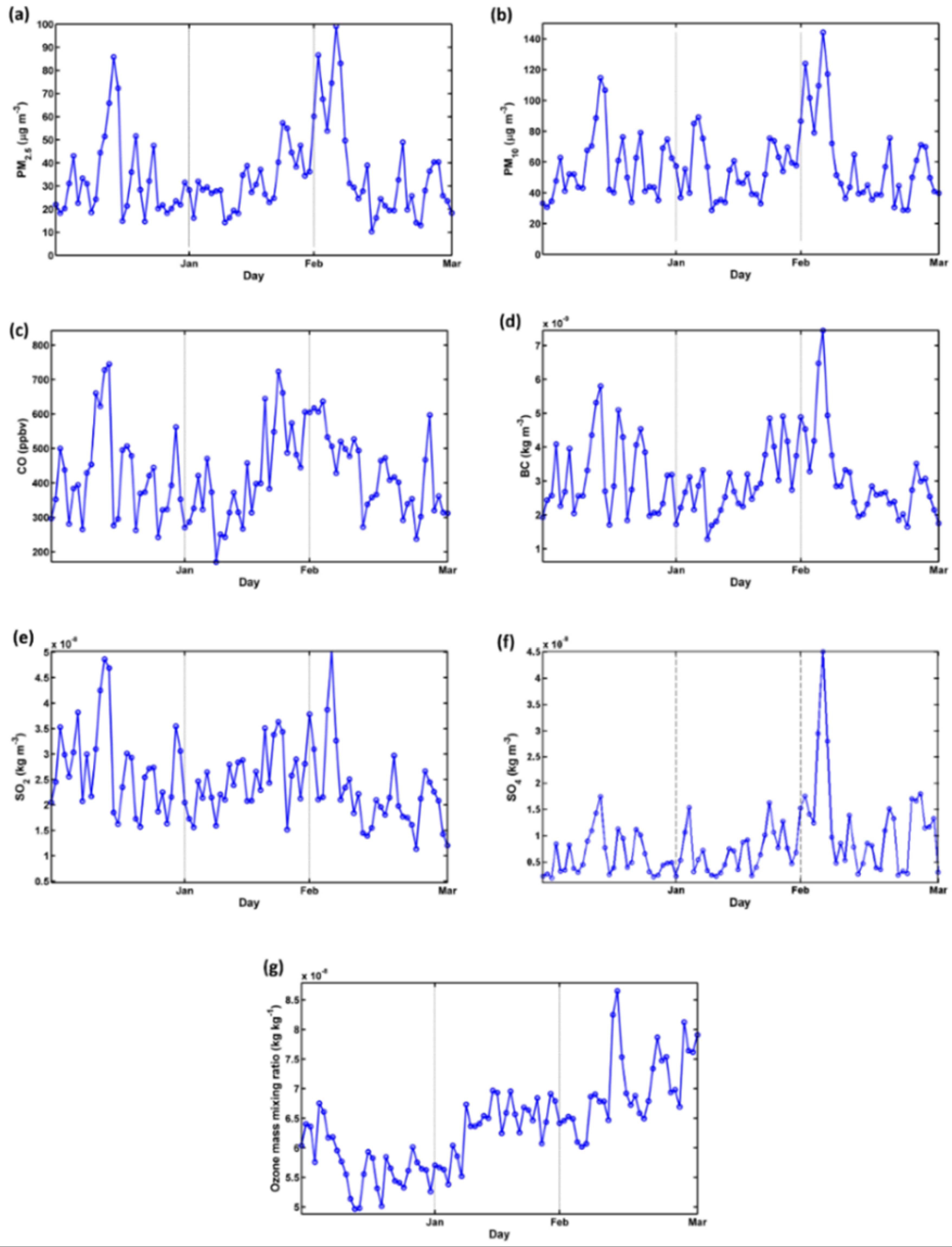
The monthly mean variability across South Korea for CO, BC, SO2, SO4, and O3 are shown in Figure 2c–g, respectively. The concentrations of CO, BC, and SO2 were high in December and January and low in July and August, similar to the annual variations in PM2.5. In contrast, SO4 and O3 levels were high in March and April and low in January and December. Peak values of CO, BC, SO2, and SO4 were detected in 2019, which were probable sources of the simultaneous high PM2.5 concentrations. To examine the haze events and pollution that caused these peak values, we described the diurnal variations in PM2.5, PM10, and other pollutants in 2019. According to the Korea Meteorological Administration, South Korea experienced two long-lasting severe haze events in 2019: the first from January 11 to 15 and the second from February 20 to March 8 (especially 1–7 March 2019) [46]. Figure 3 shows the diurnal variabilities in PM and other pollutants for January–March 2019. During these haze events, high concentrations of PM2.5 and PM10 were observed, and peak values of 99.2 μg m−3 and 144.3 μg m−3, respectively, were detected on 4–5 March 2019. The concentrations of other pollutants (CO, BC, SO2, and SO4) were also higher during these events and peaked on 4–5 March 2019. However, there was no significant variation in O3 levels. On 13–14 January 2019, PM2.5 and PM10 levels were 90 μg m−3 and 120 μg m−3, respectively. Furthermore, CO, BC, and SO2 have high peak values, whereas SO4 has a moderate peak value. The high concentrations of other pollutants support the haze events that result in high PM concentrations. Interestingly, the high and low trends of PM2.5 and PM10 were mostly consistent with CO, BC, SO2, and SO4, while O3 differed. Figure S1 shows the AOD for these haze events. High AOD values were observed on 11–15 January 2019and 1–7 March 2019and were associated with PM and other pollutant concentrations. Furthermore, AOD was highest on 14 January 2019 (0.44) and 5 March 2019 (1.19) during the first and second events, which also matched the peaked values of PM. The synoptic meteorological conditions during the severe haze events (13–14 January and 4–5 March 2019) are shown in Figure S2. During these haze events, low temperature, low-to-moderate humidity, and northwesterly/westerly winds with a WS of 5–10 m s−1 were observed in South Korea. These northwesterly/westerly winds possibly transported the pollutants from China to Korea. Figure S2 shows a high-pressure system located in South Korea and low-pressure systems located in Northern China, North Korea, and Japan. Because these low-pressure systems were extended and merged, wind flow was reduced, which resulted in the stagnation of pollutants over the region. Thus, the pollutants transported from China remained suspended for longer periods over South Korea [26,47] and were mixed with the local emissions [19]. Therefore, the high-pressure environment combined with weak vertical dispersion from winds led to PM accumulation.
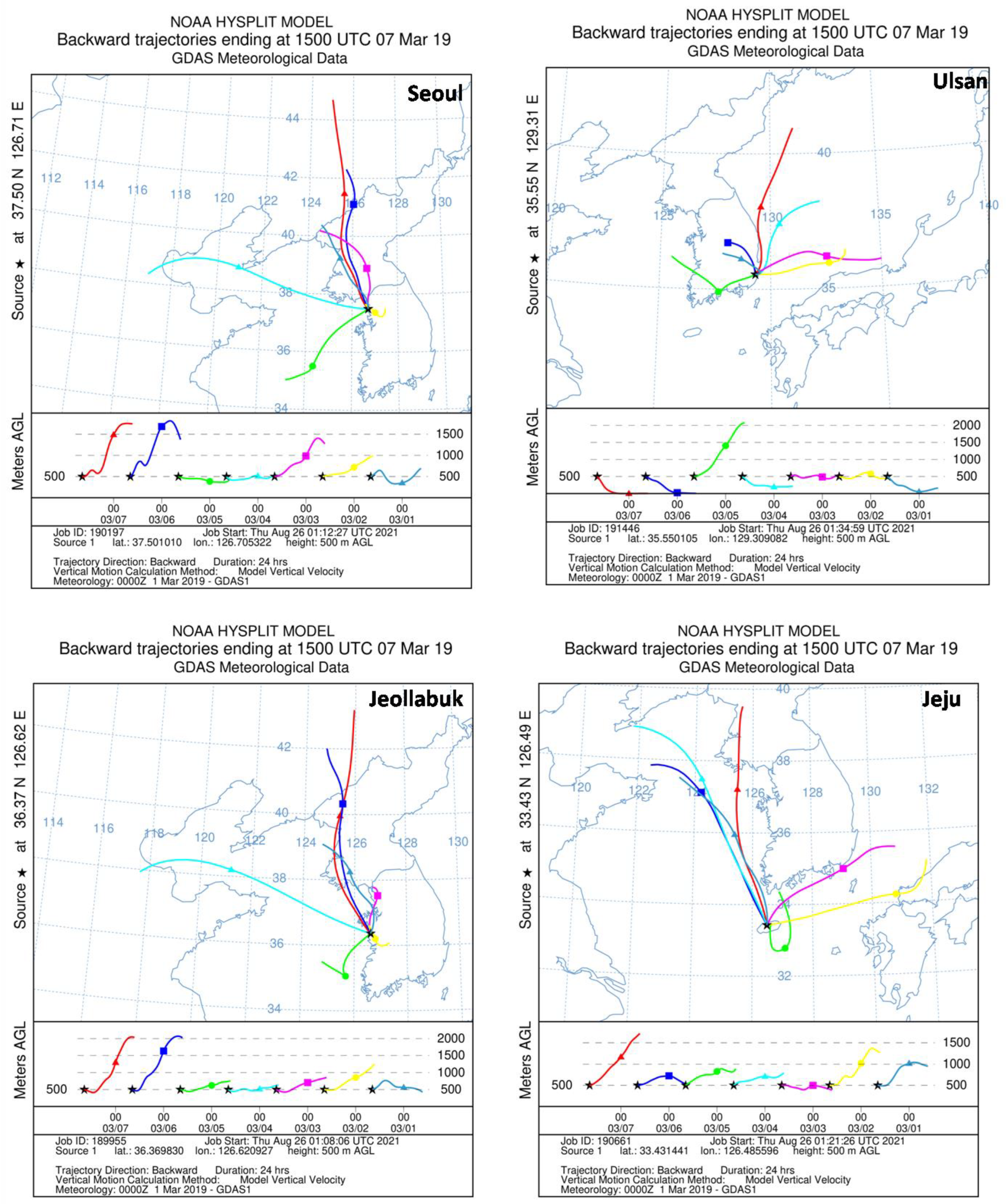
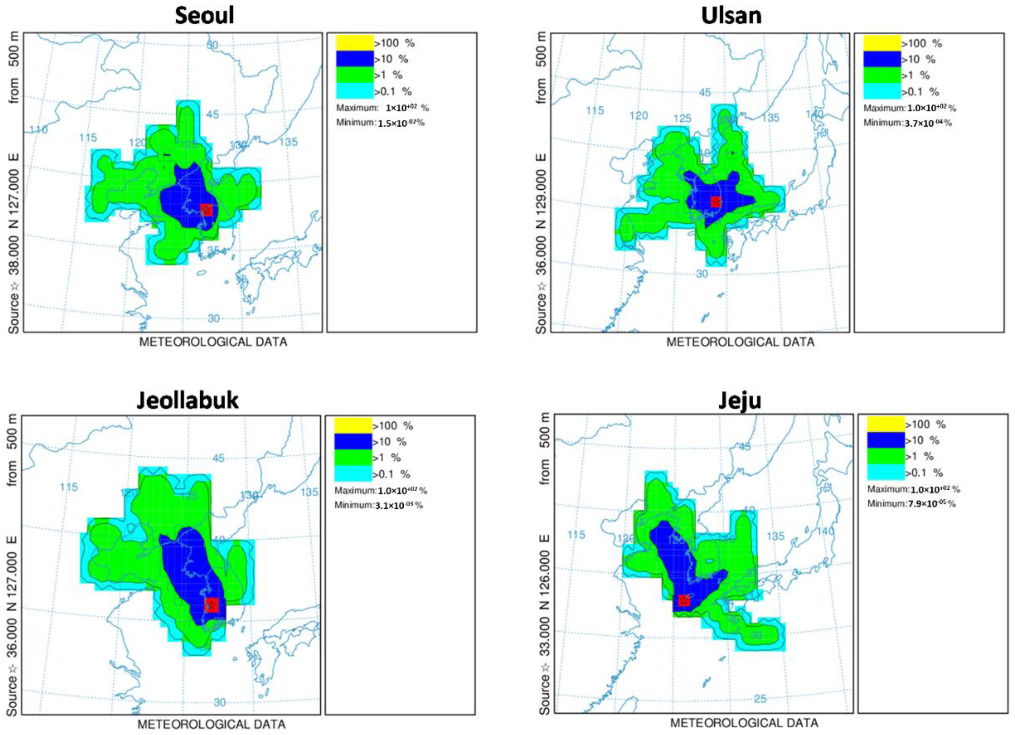
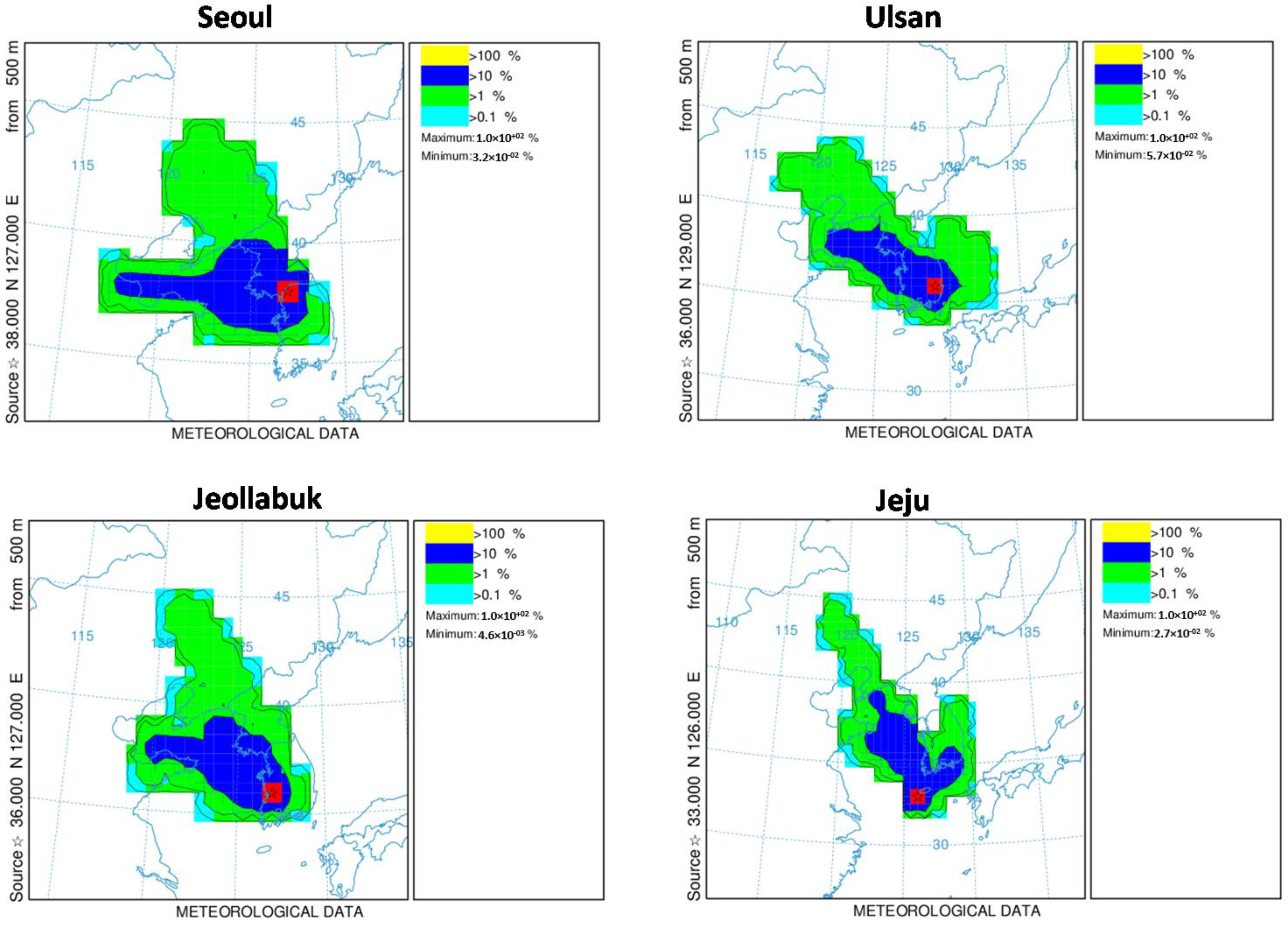
Although local pollution prevailed in South Korea, we examined the 24 h backward trajectories of air masses arriving at four sites (Seoul, Jeollabuk, Ulsan, and Jeju) from 1 to 5 March 2019to assess the impact of transboundary air pollution during heavy haze events (See Figure 4). Despite the fact that Figure 4 only shows one eastern site, two western sites, and one individual (Jeju) site, we observed trajectory patterns at all of the sites. The western sites were significantly influenced by transboundary air pollution from Eastern and Northern China; the backward trajectories show that majority of airmasses were transported from Northern China (Harbin, Jilin, and Liaoning). Interestingly, during the severe haze days (4–5 March 2019), airmasses were transported from the Beijing, Hebei, and Tianjin regions; therefore, the severe haze events were primarily caused by emissions from Eastern China. Figure 5 illustrates the trajectory frequencies and percentage of airmass transport for the four sites from February 20 to March 10. Most of the airmasses arriving in Seoul and Jeollabuk originated in Northern and Eastern China, while those in Ulsan and Jeju arrived from all directions. Figure 6 depicts the trajectory frequencies for the January haze event. Seoul and Jeollabuk have a higher percentage of airmasses transported from Eastern and Northeastern China, whereas airmasses originated primarily in Northeastern China for Ulsan and Jeju. We examined the airmass patterns during non-haze days from January to March 2020.
Figure S3 depicts the diurnal variation in PM concentrations during this time period. No severe haze events occurred in this period, and thus, peak PM concentrations did not occur as they did in January–March 2019 (Figure 3). PM concentrations were less than 60 μg m−3, and other pollutants were also in low concentrations (figure not shown). The corresponding trajectory frequencies in 2020 are shown in Figure S4 (20 February–10 March) and Figure S5 (1–15 January) for similar periods as those depicted in Figure 4 and Figure 5 (2019). Figures S4 and S5 clearly show that the majority of air masses originated in Northeastern China and the East China Sea, with no trajectories originating in Eastern China. According to the trajectory patterns for 2019 and 2020, transboundary air pollution in South Korea originated primarily in Northeast China and Mongolia. However, heavy transboundary air pollution originated mostly in Eastern China; Western Korea was also significantly influenced by this pollution.
3.2. Seasonal Variability
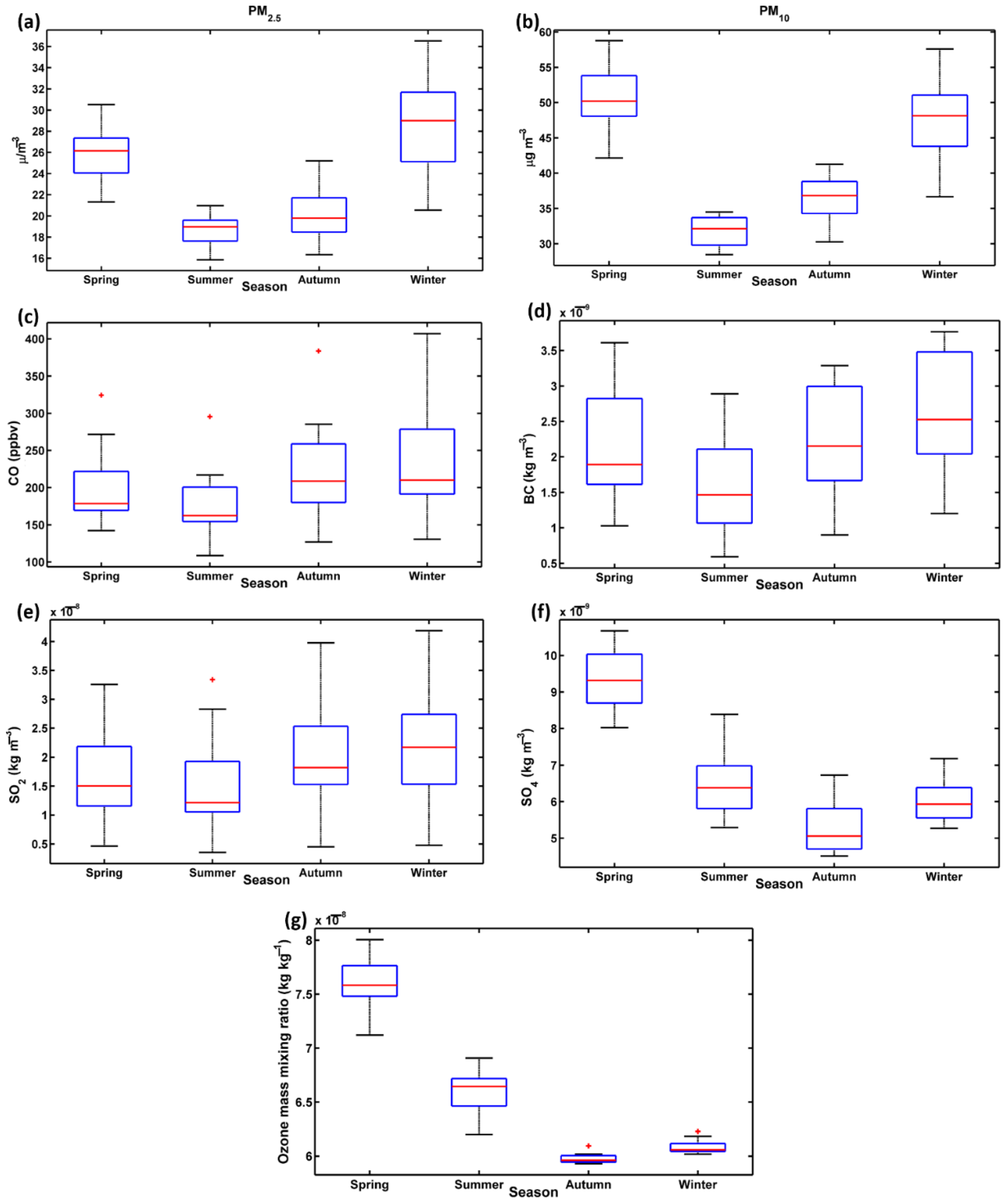
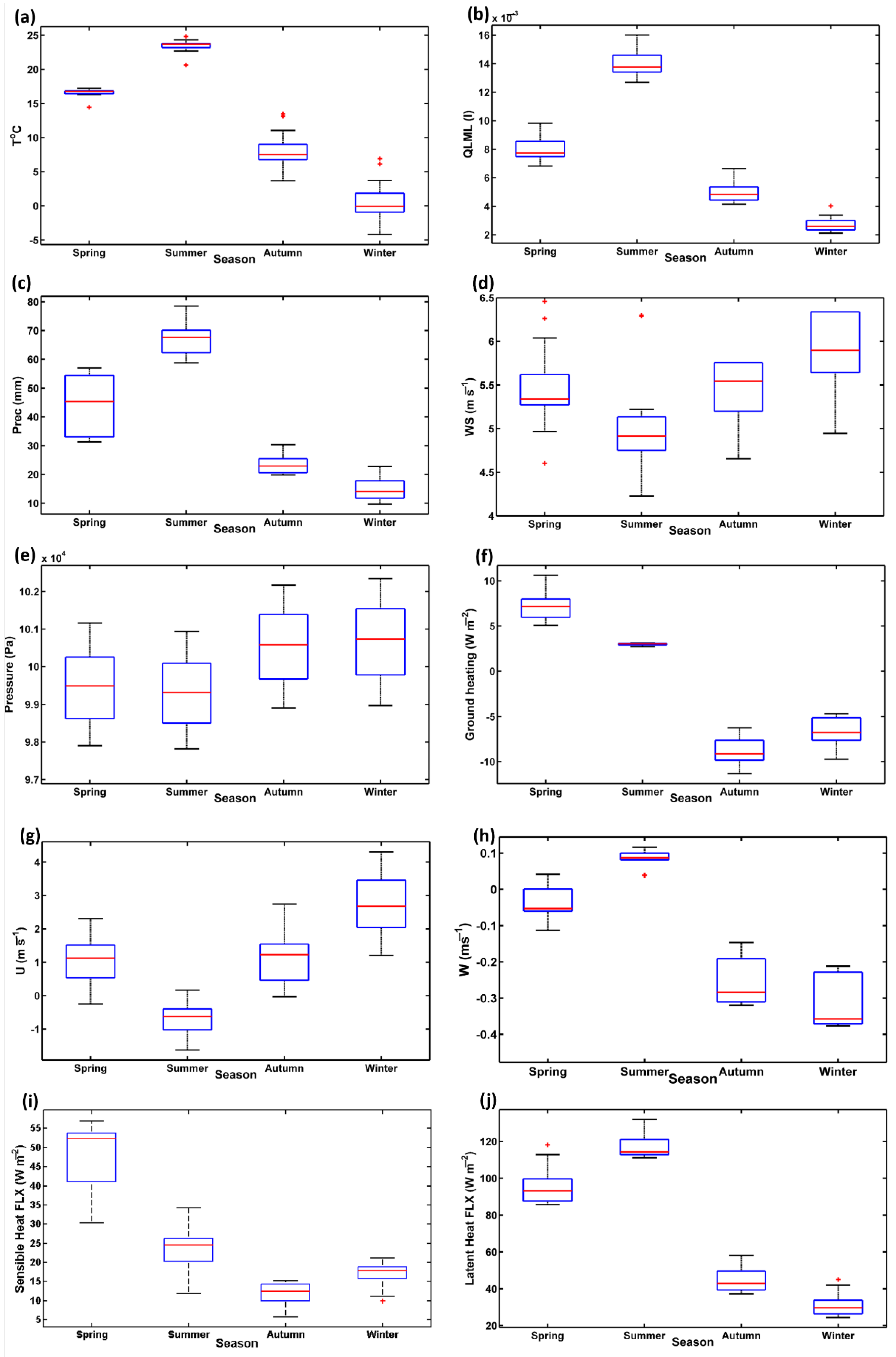
We estimated seasonal mean values for all air pollutants and PM. Figure 7 shows seasonal mean values of PM2.5, PM10, CO, BC, SO2, SO4, and O3 for the entire country. PM2.5 was the highest in winter followed by spring, autumn, and summer. CO, BC, and SO2 were also high in winter and low in summer. PM10 was the highest in spring, followed by winter, autumn, and summer. SO4 and O3 concentrations were also high in spring and interestingly, they were low during autumn. The high values of PM2.5 in winter were attributed to emissions from traffic, household heating and cooking, and industries, including coal-fired power plants, semiconductors, biopharmaceuticals, and cement [48]. The geography and climate of Korea, particularly wind direction, play an important role in PM concentration. Figure S6 shows the seasonal mean WS and direction over East Asia. Strong prevailing northwesterly winds blow over Korea from Northern China and Southern Mongolia, transporting anthropogenic emissions from these regions. In particular, the industrial regions of Harbin, Changchun, the Pearl Delta, Beijing–Tianjin, Shanghai, and Shenyang that are in Northeast and Eastern China are known to have high pollutant concentrations [2,6,13]. Thus, industrial emissions from have a significant impact on PM2.5 concentrations in Korea. During the spring, the prevailing winds are westerly and northwesterly; consequently, dust is transported to Korea from China and Mongolia, increasing PM10, O3, and SO4 concentrations. In summer, heavy precipitation reduces PM concentrations through wet removal and washing effects. Figure 2a,b show that the seasonal variation of PM concentrations decreased from 2015 to 2020.
3.3. Annual Distribution of PM and Other Pollutants
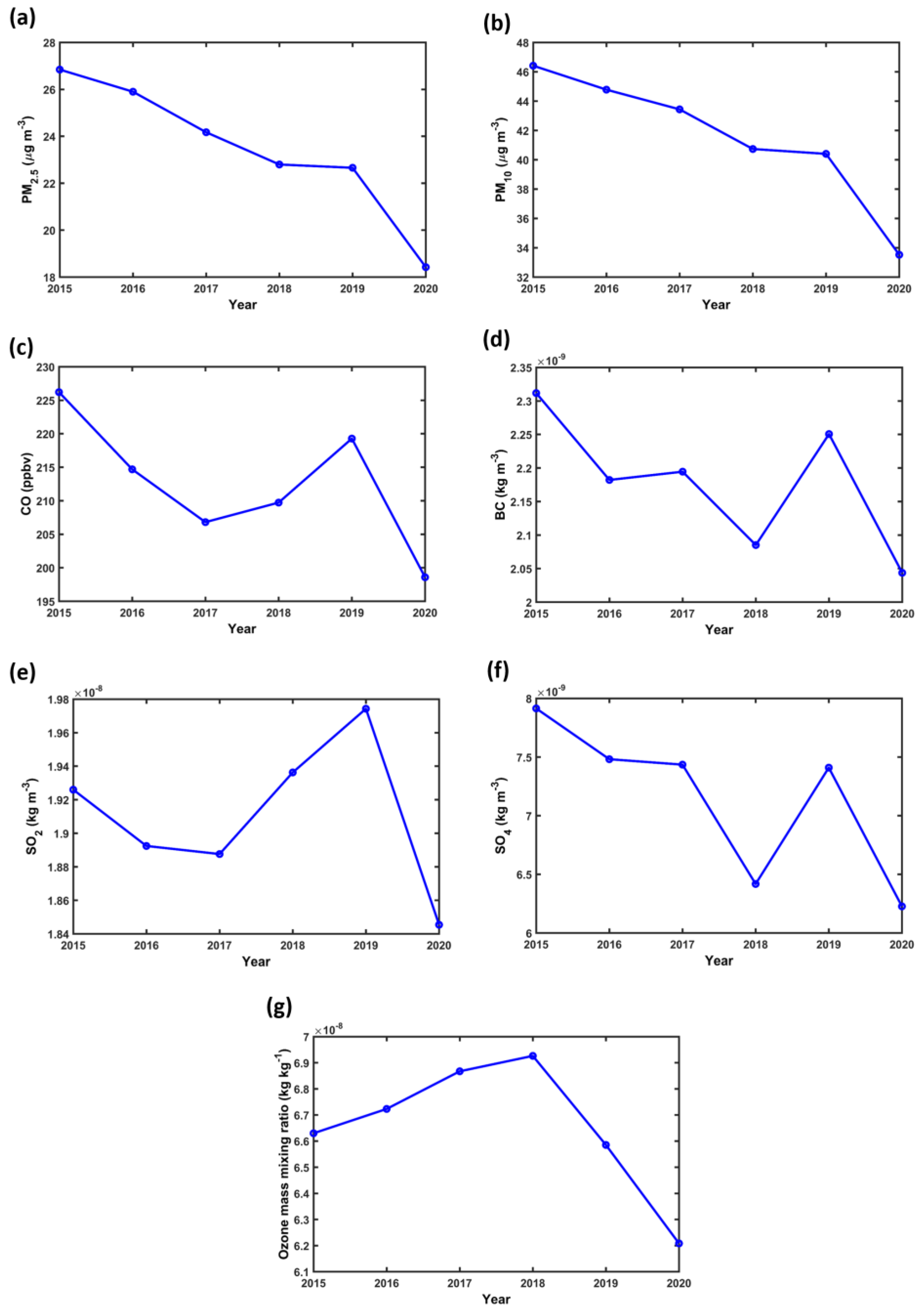
Figure 8 shows the annual mean distributions of PM and other pollutants. The South Korean government has enacted several control measures and laws to improve air quality; as a result, pollutant concentrations have decreased from 2015 to 2020. However, pollution levels in South Korea remain higher than the WHO standards. Overall, the maximum PM2.5 and PM10 concentrations were 34 μg m−3 and 54 μg m−3, respectively. Furthermore, high values were detected in 2019 due to severe haze events (as described in the previous section). The mean values of PM2.5 (PM10) were 26.8 μg m−3 (46.5 μg m−3), 25.9 μg m−3 (44.7 μg m−3), 24.1 μg m−3 (43.4 μg m−3), 22.7 μg m−3 (40.7 μg m−3), 22.6 μg m−3 (40.4 μg m−3), and 18.4 μg m−3 (33.5 μg m−3) for 2015, 2016, 2017, 2018, 2019, and 2020, respectively. CO, BC, and SO4 also tended to decrease from 2015 to 2020; however, SO2 remained mostly consistent, and O3 increased from 2015 to 2018 and then decreased.
3.4. Spatial Distribution of PM and Other Pollutants
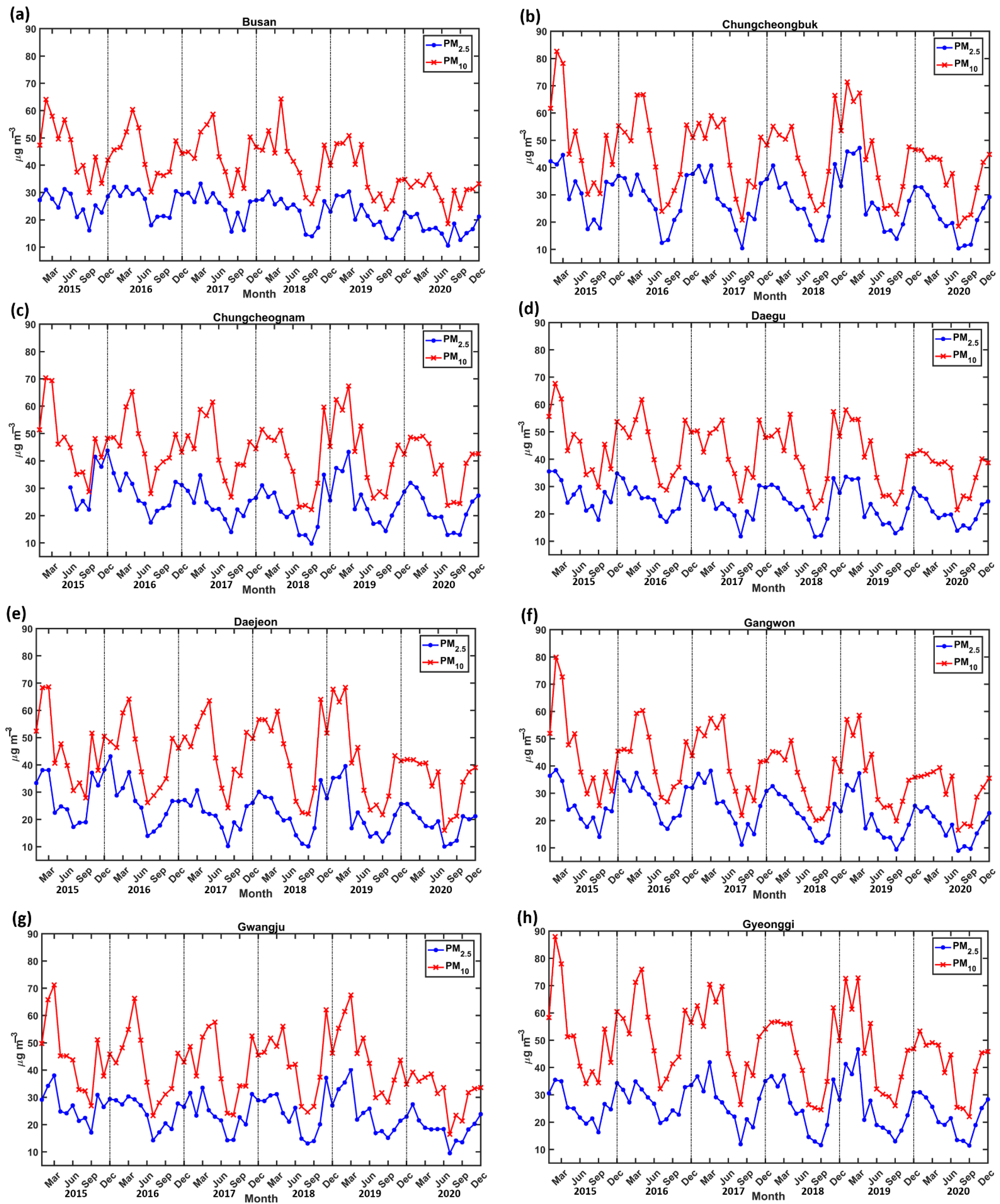
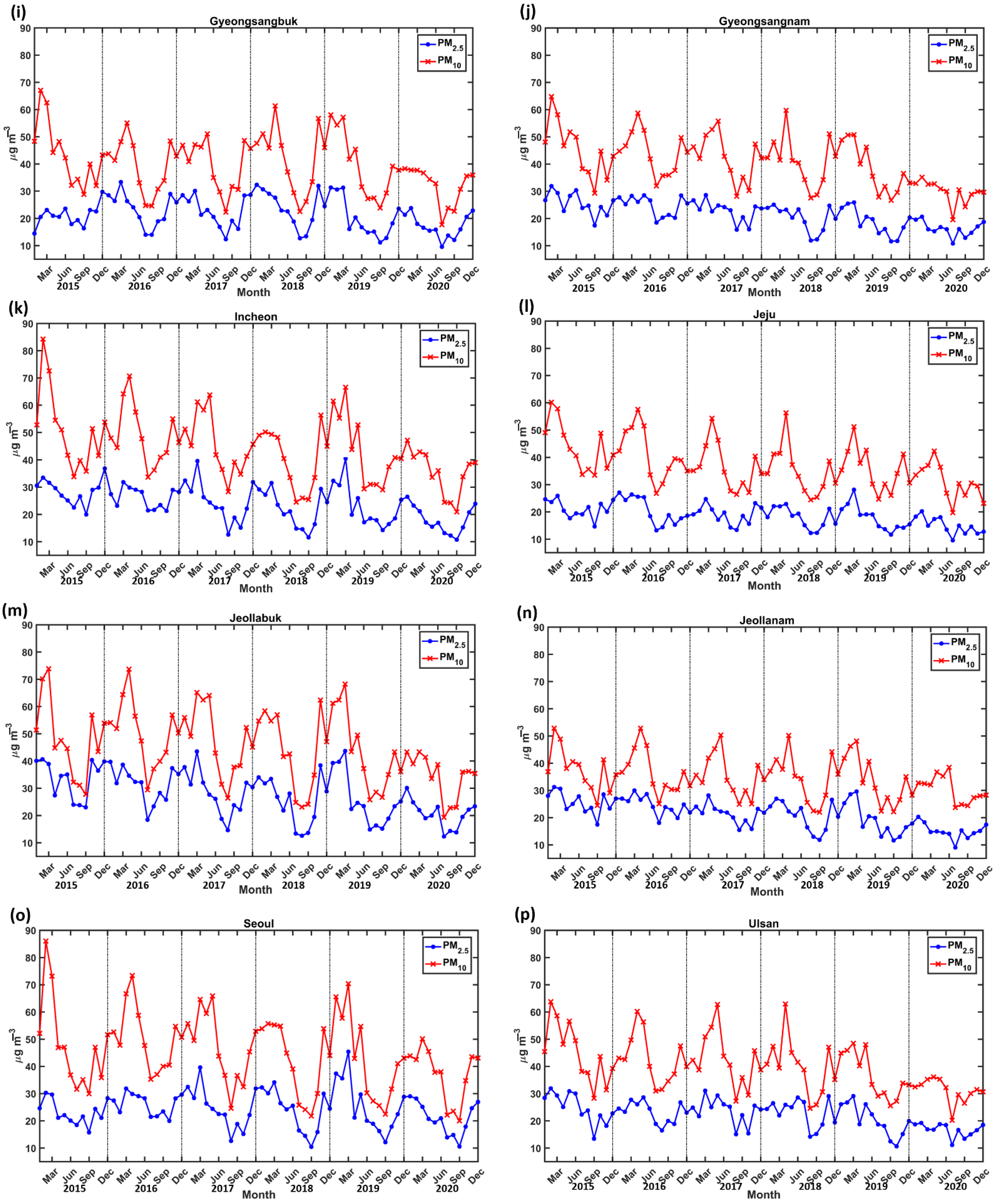
Monthly variations in PM2.5 and PM10 concentrations by administrative region are shown in Figure 9. All locations show an overall downward trend from 2015–2020. PM2.5 concentration was high during winter and low during summer. In 2019, Chungcheongbuk recorded the highest PM2.5 concentration (48.2 μg m−3), followed by Gyeonggi (47.8 μg m−3), Jeollabuk (45.4 μg m−3), and Seoul (45.3 μg m−3). These were attributed to the severe dust storm that occurred during the year. Seoul is the capital city and the largest metropolitan area in South Korea; hence, traffic volume and population density are high in the city and the surrounding Gyeonggi province. Seoul is commonly grouped with Gyeonggi and Incheon; this region is referred to as greater Seoul.
This highly urbanized area is characterized by high emissions from heavy traffic, industrial facilities, power generation, and household heating and cooking. Chungcheongbuk is located in the center of South Korea and on the southern side of the greater Seoul region. During the winter and spring, the prevailing winds from greater Seoul carry dust aerosols toward Chungcheongbuk. Furthermore, a diagonal mountain range to the southeast of Chungcheongbuk and Jeollabuk prevents further transport of these aerosols, resulting in stagnation and accumulation of pollution. Bioindustrial and semiconductor industries are in Chungcheongbuk, whereas light industries are in Jeollabuk. Consequently, PM2.5 concentrations were high in these regions. The record high PM10 concentration was in Gyeonggi (89.6 μg m−3), followed by Seoul (88.7 μg m−3) and Incheon (88.4 μg m−3) in 2015. PM10 concentrations were high in the greater Seoul area compared to Jeollabuk and Chungcheongbuk. During the spring, all stations recorded high PM10 concentrations. Interestingly, PM10 concentrations were also high in Ulsan. Because this region has the largest shipyard and numerous oil refineries, dust emissions were high. Interestingly, the southernmost regions of Korea (Jeollanam and Jeju) had the lowest PM2.5 (60 μg m−3 and PM10 (30 μg m−3) concentrations. Jeollanam lacks major industries and was less influenced by the other regions (due to its location), and Jeju island is separated from the other Korean regions and thus less affected by pollution.
3.5. Relationships between PM, Pollutant Concentrations, and Meteorological Parameters
Meteorological conditions are the primary drivers of air pollution transport and dispersion [4,6,9,10,49]. Korea is surrounded by water on three sides and 70% of the land is mountainous. Owing to its complex topography, Korea has distinctive atmospheric conditions. The mountain winds, waves, and sea breezes significantly influence the weather. Figure 10 shows the seasonal distribution of the meteorological variables in South Korea that impact air pollution. Table 1 shows Spearman’s rank correlation coefficients between the seasonal PM concentrations and pollutants and meteorological factors. The temperature was negatively correlated with both PM10 and PM2.5 in all seasons, and the relationship was significant during summer (−0.62 for PM2.5 and −0.64 for PM10). High temperatures favor intense mixing and turbulence, leading to vertical dispersion and improved air quality [33,50]. In winter, vertical dispersion was low (Figure 10h) due to more stable conditions. QLML and precipitation also had a negative correlation with both PM10 and PM2.5. The high QLML during summer promotes particle coalescence and leads to wet/dry deposition that reduces airborne PM [51]. Furthermore, high temperatures and QLML are conducive to strong convection, which causes heavy precipitation during summer. Heavy precipitation reduces PM10 concentrations because raindrops entrain particles and remove aerosols from the atmosphere. Further, wind flow affects/reduces the PM2.5 concentrations. Thus, the rainy weather can reduce PM concentrations. Therefore, PM has a stronger inverse relationship with QLML (−0.66 for PM2.5 and −0.69 for PM10) and precipitation (−0.49 for PM2.5 and −0.47 for PM10) during summer. Conversely, QLML produced weak negative correlations with PM in winter (−0.33 for PM2.5 and −0.44 for PM10), and precipitation had weak negative correlations with PM during spring (−0.15 for PM2.5 and −0.03 for PM10). Temperature, QLML, and precipitation showed significant negative correlations with PM10 during autumn (−0.71, −0.78, and −0.61, respectively). There were some interesting correlations between WS and PM concentrations; in the summer and spring, WS was negatively correlated with PM2.5 and PM10, but slightly positively correlated in the autumn and winter. Although WS was generally low during spring and summer, the W wind vector was high, which facilitated vertical pollutant dispersion. In contrast, the U wind vector was low during the summer and spring, implying that the influence of horizontal dispersion was minimal. Allabakash and Lim [33] attributed higher planetary boundary layer heights during summer and spring to upward forcing. Conversely, W was low during winter and autumn, while U was high. Therefore, horizontal PM dispersion predominated during winter and autumn [33]. Table 1 shows that U was positively correlated with PM concentration, whereas W was mostly negatively correlated. The pressure was positively correlated with both PM2.5 and PM10 in all seasons except winter. Low pressure and vertical winds during spring and summer transport PM upward. Conversely, high pressure and low vertical winds tend to accumulate PM during winter [46,50]. Interestingly, the relationship between PM and ground heating was positive in the spring, summer, and winter, but negative in the autumn. We attribute this to soil moisture content; the soil is generally dry in the spring and wet in autumn. A similar relationship was observed for latent and sensible heat fluxes. Finally, PM concentrations were positively correlated with BC, CO, SO2, and SO4 during all seasons. O3 had weak correlations with PM in spring, autumn, and winter, but a strong positive relationship during the summer.
We used the annual distributions of each parameter to determine the dominant meteorological factor influencing PM concentration. The annual mean values of the pollutants and meteorological parameters for each year are shown in Figure 8 and Figure S7, respectively. PM2.5 and PM10 concentrations decreased from 2015 to 2020, but they were higher in 2019 than in 2018 and 2020. These figures show an upward trend for all parameters with a negative relationship with PM and vice versa. However, precipitation (Figure S7c) generally shows an upward trend, except for the very dry year in 2017, which does not agree with the trends in PM concentrations. Additionally, WS (Figure S7d) shows an upward trend, indicating a negative relationship with PM. Furthermore, WS was low in 2019, which suggests an inverse relationship with PM concentration. Based on these findings, we infer that WS was the dominant meteorological factor influencing PM concentration, in line with the findings of Kim et al. [3].
3.6. Generalized Additive Model (GAM) Analysis
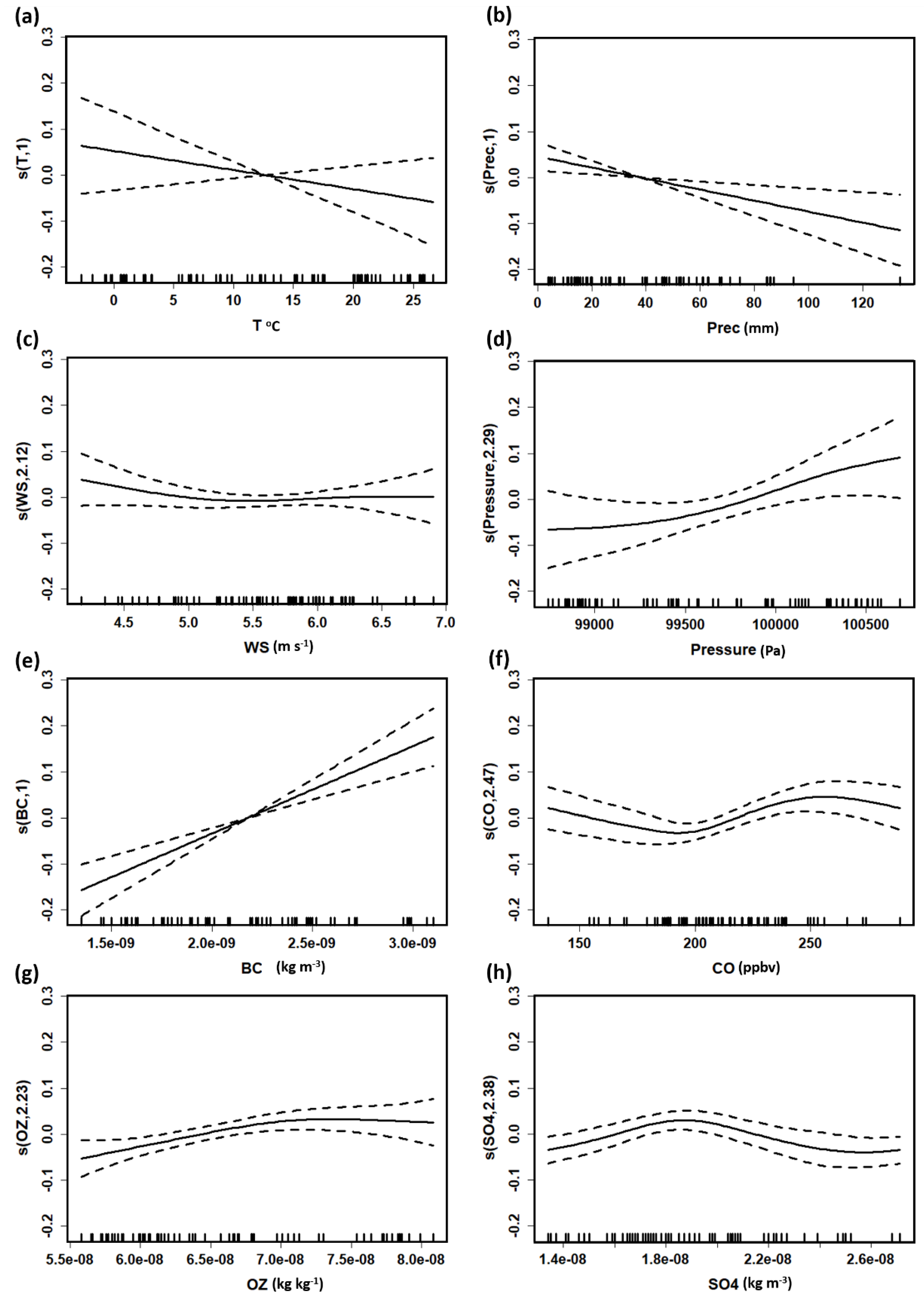
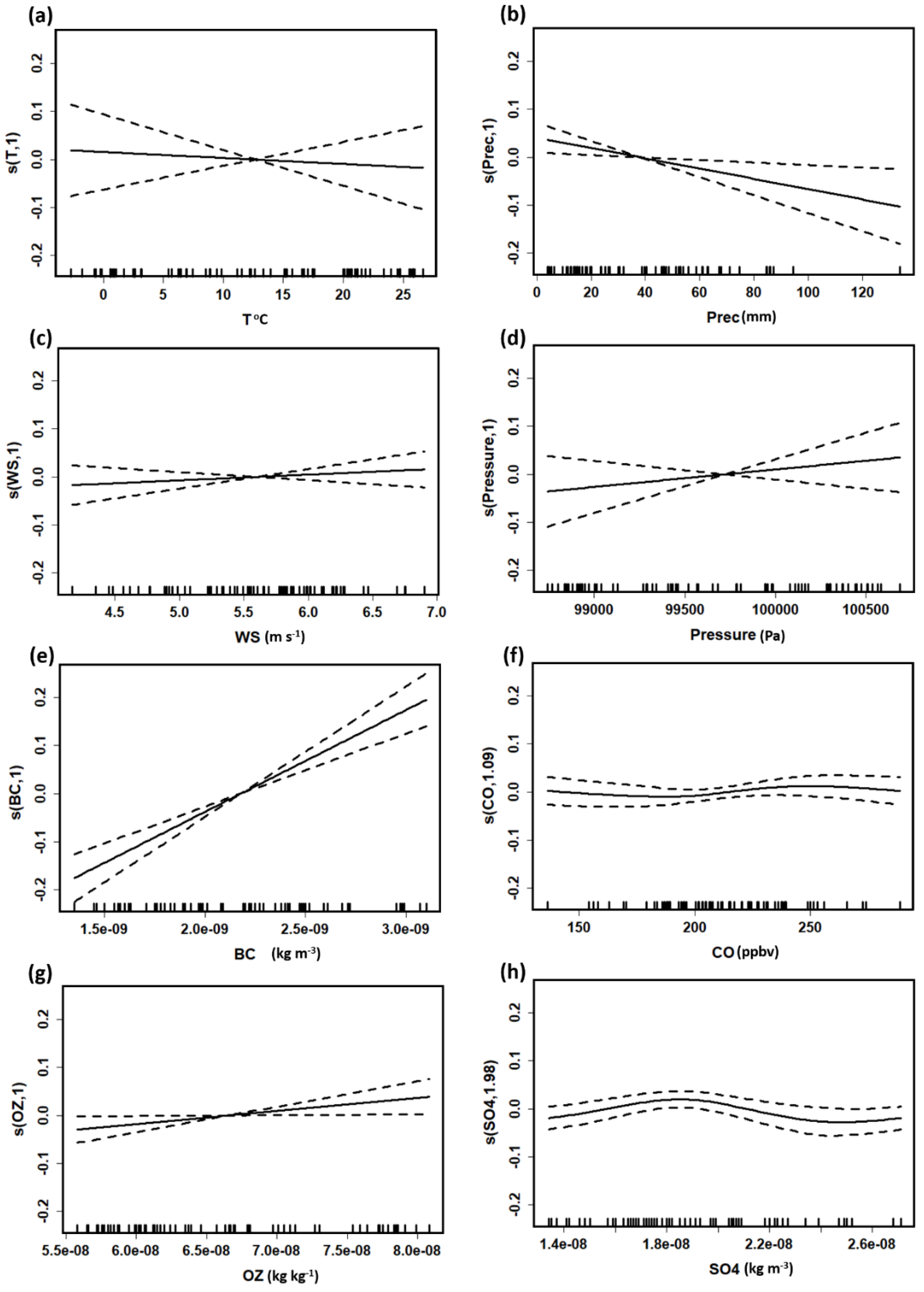
GAM was used to describe the dependencies and non-linear relationships between PM and other pollutants and meteorological factors over South Korea during 2015–2020. Figure 11 shows the relationships for PM2.5. Straight lines represent linear relationships, while curved lines represent non-linear relationships. PM2.5 shows a strong negative dependency on temperature and precipitation. PM2.5 has a negative relationship with low WS (<6 m s−1) but no clear relationship with high WS (>6 m s−1). Furthermore, PM2.5 has a strong positive relationship with pressure, BC, and O3, and a significant non-linear relationship with CO and SO4. For low CO (<200 ppbv), the relationship was stable, whereas high CO (>200 ppbv) values were positively correlated. Interestingly, PM2.5 was positively correlated with low SO4 values and weakly negatively correlated with high SO4 values. Figure 12 shows the GAM analysis for PM10 dependencies, which are broadly similar to PM2.5 dependencies. Precipitation and temperature show strong and weak negative relationships with PM10, respectively, while pressure, BC, and O3 show strong positive relationships. PM10 has a weak relationship with WS and CO. SO4 shows a non-linear relationship with PM10. Overall, the relationships between PM and meteorological factors and other pollutant were consistent with the Spearman correlations shown in Table 1.
3.7. MLR Model Analysis
Table 1 shows the linear correlations between PM, other pollutants, and meteorological factors during different seasons throughout South Korea. While the GAM model was used to describe non-linear relationships between these factors, the MLR model was used to further examine the influence of meteorological factors on pollutants at 16 sites during different seasons. The independent variables for the MLR model were selected based on their low multi-collinearity and high R2, F-test, and T-test values. Thus, QLML, P, WS, T, and precipitation were selected. The significance of the MLR model for PM2.5 passed the F-test at 15 sites, with an average R2 of 0.76 and at least four independent variables that passed the t-test. The F-test for PM10 was also passed by 15 sites, with an average R2 of 0.78 and at least four independent variables that passed the t-test. For concentrations of other pollutants (CO, BC, SO2, SO4, and O3), the MLR model passed the F-test at 13 sites with an average R2 of 0.74 and at least four independent variables that passed the t-test. The findings revealed that meteorological factors had distinct impacts in different parts of South Korea during different seasons.
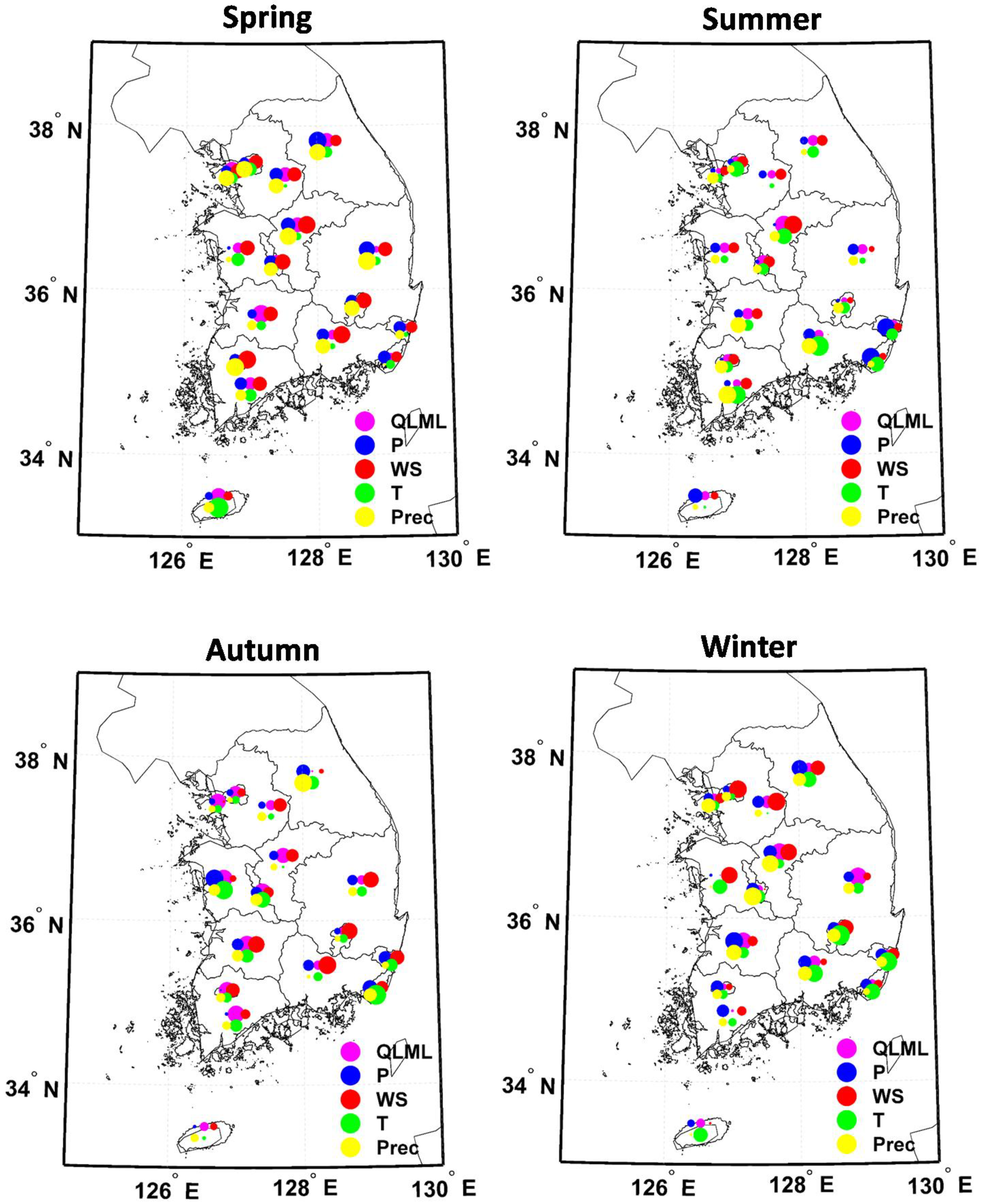
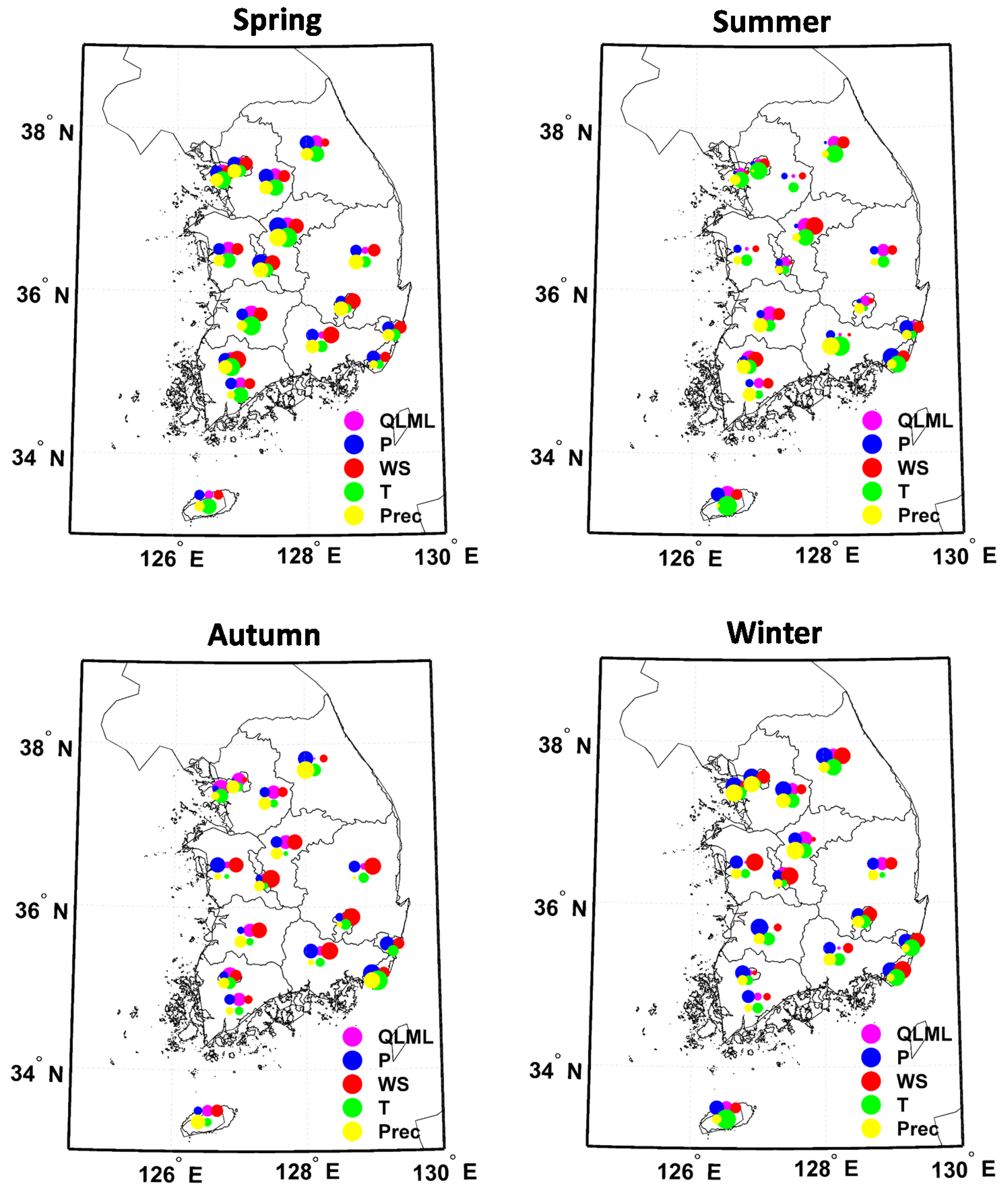
Figure 13 depicts the effect of meteorological variables on PM2.5 concentrations at all 16 sites during different seasons. During spring, WS and precipitation were the dominant factors that affected the PM2.5 concentrations at all the sites except the eastern-most sites. Pressure also played a key role in PM2.5 concentration changes over the central and eastern regions. In summer, temperature and precipitation were the dominant factors at most sites, and pressure was a significant factor at Ulsan and Busan. The WS influenced PM2.5 levels in the central and southern regions during autumn (except Seoul and surrounding regions). WS was the main contributor to PM2.5 levels in the northern and central regions (Gyeonggi and surrounding areas) during the winter. Temperature also had a strong influence on PM2.5 in the southeast. Temperature and QLML influenced PM2.5 at Jeju in the spring and winter, while pressure dominated in the summer.
The impacts of the meteorological variables on PM10 concentrations are shown in Figure 14. During spring, WS, T, precipitation, and pressure were the dominant factors that influenced the PM10 concentrations at most sites. During the summer, T and precipitation were the dominant factors in most sites, QLML and WS were dominant in the central sites, and P was dominant in the southeastern sites. PM10 in the central and eastern regions was primarily influenced by WS; however, P was also influencing PM10 over the eastern sites during autumn. In winter, WS was the dominant factor influencing PM10 in Seoul, Jeollabuk, Gyengsonbuk, Daejon, Ulsan, Busan, and Daegu during the winter. T and P were the dominant factors that influenced PM10 concentrations in Jeju during spring, summer, and winter, while precipitation, WS, and QLML influenced PM10 concentrations in autumn. Figure S8 shows the impacts of the meteorological factors on CO. WS, T, P, and precipitation were the dominant factors impacting CO concentrations during all seasons at Seoul. Further, pressure significantly affected CO at all sites during all seasons. Over southeastern sites, T, P, and WS were dominant in the spring, and T and P were dominant in the winter, and these factors influence CO concentrations. In Jeju, CO concentration was influenced by T and P during spring and winter. However, WS was dominant in summer, and T and QLML were dominant during autumn. Figure S9 shows that, BC concentrations were significantly influenced by all the meteorological factors in the western part of Korea, but their influence was less in the east during all seasons. In Jeju, T was the dominant factor for BC concentration during all seasons. Furthermore, P and precipitation impacted the BC concentration during summer, while QLML impacted it during autumn and winter. Figure S10 shows the impacts of the meteorological factors on SO4; they were mostly similar to those on BC. Figure S11 shows that the SO2 concentrations over northwestern regions (especially the Seoul metropolitan region) were influenced by all meteorological factors, especially WS and precipitation, during all seasons. In Jeju, SO2 was mostly influenced by T. SO2 at the central sites was less affected by meteorological parameters during the summer. Figure S12 shows that the O3 concentrations during spring were influenced by all the meteorological factors (mainly T, precipitation, and WS) in the western and southern regions. During the summer, all meteorological factors influenced O3 concentrations in the northwest (Seoul and surrounding areas). Meteorological factors influenced O3 concentrations at all sites during the autumn and winter seasons. O3 concentrations in Jeju were influenced by T, P, and QLML during all seasons.
4. Conclusions
We analyzed the spatial and temporal variability in PM2.5 and PM10 over South Korea during 2015–2020, as well as the relationship between PM, other pollutants, and meteorological parameters. The highest nationally averaged PM2.5 concentrations were observed during December and January, and the highest PM10 concentrations were observed during March and April. PM2.5 and PM10 were the lowest during July and August. Seasonal patterns revealed that PM2.5 levels were highest in winter, then in spring, autumn, and summer. CO, BC, and SO2 concentrations peaked as well during the winter. In contrast, PM10, SO4, and O3 were highest in the spring and lowest in the summer. High PM concentrations were attributed to emissions from traffic, household heating and cooking, and industries during the winter and spring. During spring and winter, the prevailing westerly and northwesterly winds were relatively strong and transported anthropogenic emissions and dust to Korea from China and Mongolia. The greater Seoul region is characterized by high traffic, population density, and various industrial facilities; therefore, high PM10 and PM2.5 concentrations were recorded in the region. CO, BC, SO2, and SO4 were also high over the greater Seoul region. The highest PM2.5 concentrations were observed over Chungcheongbuk and Jeollabuk due to emissions from biological, semiconductor, and light industries in these provinces. Furthermore, prevailing winds carried emissions from greater Seoul to Chungcheongbuk and Jeollabuk. Western South Korea had higher PM and pollutant concentrations than the eastern regions due to its proximity to China. Due to the occurrence of two heavy haze events in 2019, pollution was high, which was aided by high AOD values. The back trajectories of the Hysplit model described how emissions from Eastern China sources significantly influence pollution in Korea during haze events. The Jeju site was less influenced by foreign pollution. We explored the relationships between PM2.5 and PM10, meteorological parameters, and other pollutants. PM2.5 and PM10 concentrations showed negative correlations with temperature, QLML, and precipitation in all seasons. During summer, PM2.5 and PM10 had strong negative correlations with temperature, QLML, and precipitation. Temperature and QLML tend to be high during summer, and these warm and humid conditions were conducive to strong convection and precipitation. Under heavy precipitation, the wet scavenging effect reduced PM concentrations. During the summer and spring, PM2.5 and PM10 were inversely related to WS. During these seasons, W was high, and U was low, promoting vertical pollutant dispersion. Conversely, horizontal winds predominated during autumn and winter and horizontal dispersion was the primary driver modulating PM concentrations. PM2.5 and PM10 were positively correlated with pressure during all seasons except winter. PM is transported upwards by low pressure and high W, whereas PM is accumulated by high pressure and low W. PM was positively correlated with ground heating during all seasons, except autumn, which was attributed to varying seasonal soil moisture content. PM concentrations were positively correlated with CO, BC, SO2, and SO4 in all seasons. A GAM analysis was conducted to identify PM concentration dependencies on meteorological parameters and other pollutants. Furthermore, the MLR model demonstrated the impact of meteorological parameters on PM concentrations and other pollutants at each site throughout the seasons. Spearman’s rank correlation, GAM, and MLR were used to investigate the relationship between meteorological factors and PM concentrations, as well as the dominant influencing factors and their effect on pollution levels in each region of Korea during different seasons.
The primary focus of this study was the relationship between meteorological factors and PM concentrations during different months and seasons. However, in the future, we will conduct a separate study to examine the contributions of foreign/transboundary and local air pollution in Korea for various meteorological conditions/events using WRF, CMAQ, and other chemical models.
Supplementary Materials
The following supporting information can be downloaded at: https://www.mdpi.com/article/10.3390/rs14194849/s1, Figure S1: Diurnal distribution of aerosol optical depth (AOD) during the severe haze events in (a) January and (b) February–March in 2019. The vertical dotted line in (b) indicates the separation between the two months; Figure S2: (a) Surface temperature and relative humidity profiles and (b) surface pressure and wind profiles on 13–14 January 2019; the dashed lines indicate isotherms. (c) Surface temperature and relative humidity profiles and (d) surface pressure and wind profiles on 4–5 March 2019. The dashed lines indicate isotherms, the white spaces represent the absence of data, and the solid-colored lines represent isobars; Figure S3: Diurnal distribution of the particulate matter (PM) concentration from January to March 2020. (a) PM2.5 concentrations and (b) PM10 concentrations; Figure S4: Trajectory frequencies (percentage of airmass transport) over the four sites during 20 February–10 March 2020; Figure S5: Trajectory frequencies (percentage of airmass transport) over the four sites during 1–15 January 2020; Figure S6: Spatial distribution of seasonal mean wind speed (m s−1) and direction over East Asia (2015–2020). (a) spring, (b) summer, (c) autumn, and (d) winter; Figure S7: Mean annual distribution of the meteorological parameters impacting air pollution in South Korea (2015–2020). The straight red line indicates the linear fit of the values. (a) temperature, (b) specific humidity, (c) precipitation, (d) wind speed, (e) pressure, (f) ground heating, (g) horizontal (zonal) wind vector, (h) vertical wind vector, (i) sensible heat flux, and (j) latent heat flux; Figure S8: MLR model results between CO and the meteorological parameters. The colors represent the type of the meteorological parameter, and the size indicates the magnitude of the influencing parameter. R2 represents the fitting effect of the model, the F-test determines the significance of the model, and the t-test determines the significance of the independent variables; Figure S9: MLR model results between BC and the meteorological parameters. The colors represent the type of the meteorological parameter, and the size indicates the magnitude of the influencing parameter. R2 represents the fitting effect of the model, the F-test determines the significance of the model, and the t-test determines the significance of the independent variables; Figure S10: MLR model results between SO4 and the meteorological parameters. The colors represent the type of the meteorological parameter, and the size indicates the magnitude of the influencing parameter. R2 represents the fitting effect of the model, the F-test determines the significance of the model, and the t-test determines the significance of the independent variables; Figure S11: MLR model results between SO2 and the meteorological parameters. The colors represent the type of the meteorological parameter and size indicates the magnitude of the influencing parameter. R2 represents the fitting effect of the model, the F-test determines the significance of the model, and the t-test determines the significance of the independent variables; Figure S12: MLR model results between O3 and the meteorological parameters. The colors represent the type of the meteorological parameter, and the size indicates the magnitude of the influencing parameter. R2 represents the fitting effect of the model, the F-test determines the significance of the model, and the t-test determines the significance of the independent variables.
Author Contributions
S.A. performed data analyses and conceptualization and wrote the first manuscript draft. S.L. provided helpful discussions on the analyses of data, conceptualization, methodology, and review and edited the manuscript. K.-S.C. and T.J.Y. reviewed and edited the manuscript. All authors have read and agreed to the published version of the manuscript.
Funding
Research for this paper was carried out under the KICT Research Program (20220136-001, Development of 3D Fine Dust Estimating Technology based on AI Image Analysis) funded by the Ministry of Science and ICT.
Data Availability Statement
The PM2.5 data used in the present study are available at Air Korea, https://www.airkorea.or.kr/web/pmRelay?itemCode=10007&pMENU_NO=108 (accessed on 8 July 2021). The data used for meteorological parameters and other pollutants is available at MERRA-2, https://disc.sci.gsfc.nasa.gov/datasets?keywords=%22MERRA-%22&page=1&source=Models%2FAnalyses%20MERRA-2 (accessed on 10 July 2021).
Acknowledgments
The authors would like to thank GMAO NASA for providing the MERRA-2 surface datasets used in this study.
Conflicts of Interest
The authors declare no conflict of interest.
References
- Monks, P.; Granier, C.; Fuzzi, S.; Stohl, A.; Williams, M.; Akimoto, H.; Amann, M.; Baklanov, A.; Baltensperger, U.; Bey, I.; et al. Atmospheric composition change–global and regional air quality. Atmos. Environ. 2009, 43, 5268–5350. [Google Scholar] [CrossRef]
- Zhu, W.; Xu, X.; Zheng, J.; Yan, P.; Wang, Y.; Cai, W. The characteristics of abnormal wintertime pollution events in the Jing-Jin-Ji region and its relationships with meteorological factors. Sci. Total Environ. 2018, 626, 887–898. [Google Scholar] [CrossRef] [PubMed]
- Kim, H.C.; Kim, S.; Kim, B.-U.; Jin, C.-S.; Hong, S.; Park, R.; Son, S.-W.; Bae, C.; Bae, M.; Song, C.-K.; et al. Recent increase of surface particulate matter concentrations in the Seoul Metropolitan Area, Korea. Sci. Rep. 2017, 7, 1–7. [Google Scholar] [CrossRef] [PubMed]
- Kliengchuay, W.; Cooper Meeyai, A.; Worakhunpiset, S.; Tantrakarnapa, K. Relationships between meteorological parameters and particulate matter in Mae Hong Son Province, Thailand. Int. J. Environ. Res. Public Health. 2018, 15, 2801. [Google Scholar] [CrossRef] [PubMed]
- Ocak, S.; Turalioglu, F.S. Effect of meteorology on the atmospheric concentrations of traffic-related pollutants in Erzurum, Turkey. J. Int. Environ. Appl. Sci. 2008, 3, 325–335. [Google Scholar]
- Zhang, H.; Wang, Y.; Hu, J.; Ying, Q.; Hu, X.M. Relationships between meteorological parameters and criteria air pollutants in three megacities in China. Environ. Res. 2015, 140, 242–254. [Google Scholar] [CrossRef]
- Cao, Q.; Pui, D.Y.; Lipinski, W. A concept of a novel solar-assisted large-scale cleaning system (SALSCS) for urban air remediation. Aerosol Air Qual. Res. 2014, 15, 1–10. [Google Scholar] [CrossRef]
- Guo, H.; Jiang, F.; Cheng, H.R.; Simpson, I.J.; Wang, X.M.; Ding, A.J.; Wang, T.J.; Saunders, S.M.; Lam, S.H.M.; Blake, D.R. Concurrent observations of air pollutants at two sites in the Pearl River Delta and the implication of regional transport. Atmos. Chem. Phys. 2009, 9, 7343–7360. [Google Scholar] [CrossRef]
- Haddad, K.; Vizakos, N. Air quality pollutants and their relationship with meteorological variables in four suburbs of Greater Sydney, Australia. Air Qual. Atmos. Health 2021, 14, 55–67. [Google Scholar] [CrossRef]
- Jassim, M.S.; Coskuner, G.; Munir, S. Temporal analysis of air pollution and its relationship with meteorological parameters in Bahrain, 2006–2012. Arab. J. Geosci. 2018, 11, 1–15. [Google Scholar] [CrossRef]
- Sharma, A.P.; Kim, K.; Ahn, J.; Shon, Z.; Sohn, J.; Lee, J.; Ma, C.; Brown, R.J. Ambient particulate matter (PM10) concentrations in major urban areas of Korea during 1996–2010. Atmos. Poll. Res. 2014, 5, 161–169. [Google Scholar] [CrossRef] [Green Version]
- Liu, Y.; Zhou, Y.; Lu, J. Exploring the relationship between air pollution and meteorological conditions in China under environmental governance. Sci. Rep. 2020, 10, 1–11. [Google Scholar]
- Li, X.; Ma, Y.; Wang, Y.; Liu, N.; Hong, Y. Temporal and spatial analyses of particulate matter (PM10 and PM2.5) and its relationship with meteorological parameters over an urban city in northeast China. Atmos. Res. 2017, 198, 185–193. [Google Scholar] [CrossRef]
- Caramagna, A.; Famoso, F.; Lanzafame, R.; Monforte, P. Analysis of vertical profile of particulates dispersion in function of the aerodynamic diameter at a congested road in Catania. Energy Procedia 2015, 82, 702–707. [Google Scholar] [CrossRef]
- Brusca, S.; Famoso, F.; Lanzafame, R.; Garrano, A.M.C.; Monforte, P. Experimental analysis of a plume dispersion around obstacles. Energy Procedia 2015, 82, 695–701. [Google Scholar] [CrossRef]
- Crawford, J.H.; Ahn, J.-Y.; Al-Saadi, J.; Chang, L.; Emmons, L.K.; Kim, J.; Lee, G.; Park, J.-H.; Park, R.J.; Woo, J.H.; et al. The Korea–United States Air Quality (KORUS-AQ) field study. Elem. Sci. Anth. 2021, 9, 00163. [Google Scholar] [CrossRef]
- Jordan, C.E.; Crawford, J.H.; Beyersdorf, A.J.; Eck, T.F.; Halliday, H.S.; Nault, B.A.; Chang, L.S.; Park, J.; Park, R.; Lee, G.; et al. Investigation of factors controlling PM2.5 variability across the South Korean Peninsula during KORUS-AQ. Elementa-Sci. Anthrop. 2020, 8. [Google Scholar] [CrossRef]
- Eck, T.F.; Holben, B.; Kim, J.; Beyersdorf, A.; Choi, M.; Lee, S.; Koo, J.-H.; Giles, D.; Schafer, J.; Sinyuk, A.; et al. Influence of cloud, fog, and high relative humidity during pollution transport events in South Korea: Aerosol properties and PM2.5 variability. Atmos. Environ. 2020, 232, 117530. [Google Scholar] [CrossRef]
- Peterson, D.A.; Hyer, E.J.; Han, S.-O.; Crawford, J.H.; Park, R.J.; Holz, R.; Kuehn, R.E.; Eloranta, E.; Knote, C.; Jordan, C.; et al. Meteorology influencing springtime air quality, pollution transport, and visibility in Korea. Elementa-Sci. Anthr. 2019, 7, 57. [Google Scholar] [CrossRef]
- Kumar, N.; Park, R.J.; Jeong, J.I.; Woo, J.H.; Kim, Y.; Johnson, J.; Yarwood, G.; Kang, S.; Chun, S.; Knipping, E. Contributions of international sources to PM2. 5 in South Korea. Atmos. Environ. 2021, 261, 118542. [Google Scholar] [CrossRef]
- Xie, P.; Liao, H. The Impacts of Changes in Anthropogenic Emissions Over China on PM2. 5 Concentrations in South Korea and Japan During 2013–2017. Front. Environ. Sci. 2022, 31, 1–14. [Google Scholar]
- Lee, S.; Kim, J.; Choi, M.; Hong, J.; Lim, H.; Eck, T.F.; Holben, B.N.; Ahn, J.Y.; Kim, J.; Koo, J.H. Analysis of long-range transboundary transport (LRTT) effect on Korean aerosol pollution during the KORUS-AQ campaign. Atmos. Environ. 2019, 204, 53–67. [Google Scholar] [CrossRef]
- Yim, S.H.L.; Gu, Y.; Shapiro, M.A.; Stephens, B. Air quality and acid deposition impacts of local emissions and transboundary air pollution in Japan and South Korea. Atmos. Chem. Phys. 2019, 19, 13309–13323. [Google Scholar] [CrossRef] [Green Version]
- Choi, J.; Park, R.J.; Lee, H.M.; Lee, S.; Jo, D.S.; Jeong, J.I.; Henze, D.K.; Woo, J.H.; Ban, S.J.; Lee, M.D.; et al. Impacts of local vs. trans-boundary emissions from different sectors on PM2. 5 exposure in South Korea during the KORUS-AQ campaign. Atmos. Environ. 2019, 203, 196–205. [Google Scholar] [CrossRef]
- Park, S.K. Seasonal variations of fine particulate matter and mortality rate in Seoul, Korea with a focus on the short-term impact of meteorological extremes on human health. Atmosphere 2021, 12, 151. [Google Scholar] [CrossRef]
- Han, S.B.; Song, S.K.; Shon, Z.H.; Kang, Y.H.; Bang, J.H.; Oh, I. Comprehensive study of a long-lasting severe haze in Seoul megacity and its impacts on fine particulate matter and health. Chemosphere 2021, 268, 129369. [Google Scholar] [CrossRef] [PubMed]
- Lee, S.; Ho, C.H.; Choi, Y.S. High-PM10 concentration episodes in Seoul, Korea: Background sources and related meteorological conditions. Atmos. Environ. 2011, 45, 7240–7247. [Google Scholar] [CrossRef]
- Lee, S.; Ho, C.H.; Lee, Y.G.; Choi, H.J.; Song, C.K. Influence of transboundary air pollutants from China on the high-PM10 episode in Seoul, Korea for the period October 16–20, 2008. Atmos. Environ. 2013, 77, 430–439. [Google Scholar] [CrossRef]
- Allabakash, S.; Lim, S. Anthropogenic influence of temperature changes across East Asia using CMIP6 simulations. Sci. Rep. 2022, 12, 1–14. [Google Scholar] [CrossRef]
- Available online: https://seoulsolution.kr/en/content/6540 (accessed on 8 July 2021).
- Available online: https://www.airkorea.or.kr/web/pmRelay?itemCode=10007&pMENU_NO=108 (accessed on 8 July 2021).
- Kim, H.G.; Kim, J.Y.; Kang, Y.H. Comparative evaluation of the third-generation reanalysis data for wind resource assessment of the southwestern offshore in South Korea. Atmosphere 2018, 9, 73. [Google Scholar] [CrossRef]
- Allabakash, S.; Lim, S. Climatology of Planetary Boundary Layer Height-Controlling Meteorological Parameters Over the Korean Peninsula. Remote Sens. 2020, 12, 2571. [Google Scholar] [CrossRef]
- Allabakash, S.; Lim, S.; Chandrasekar, V.; Min, K.H.; Choi, J.; Jang, B. X-band dual-polarization radar observations of snow growth processes of a severe winter storm: Case of 12 December 2013 in South Korea. J. Atmos. Ocean. Technol. 2019, 36, 1217–1235. [Google Scholar] [CrossRef]
- Bosilovich, M.; Akella, S.; Coy, L.; Cullather, R.; Draper, C.; Gelaro, R.; Kovach, R.; Liu, Q.; Molod, A.; Norris, P.; et al. MERRA-2: Initial Evaluation of the Climate; NASA Tech. Rep. Series on Global Modeling and Data Assimilation; NASA/TM–2015-104606, 43; NASA Goddard Space Flight Center: Greenbelt, MD, USA, 2015.
- Pearce, J.L.; Beringer, J.; Nicholls, N.; Hyndman, R.J.; Tapper, N.J. Quantifying the influence of local meteorology on air quality using generalized additive models. Atmos. Environ. 2011, 45, 1328–1336. [Google Scholar] [CrossRef]
- Bertaccini, P.; Dukic, V.; Ignaccolo, R. Modeling the short-term effect of traffic and meteorology on air pollution in Turin with generalized additive models. Adv. Meteorol. 2012, 2012, 609328. [Google Scholar] [CrossRef]
- Carslaw, D.C.; Beevers, S.D.; Tate, J.E. Modelling and assessing trends in traffic-related emissions using a generalised additive modelling approach. Atmos. Environ. 2007, 41, 5289–5299. [Google Scholar] [CrossRef]
- Huang, F.; Li, X.; Wang, C.; Xu, Q.; Wang, W.; Luo, Y.; Tao, L.; Gao, Q.; Guo, J.; Chen, S.; et al. PM2.5 spatiotemporal variations and the relationship with meteorological factors during 2013–2014 in Beijing, China. PLoS ONE 2015, 10, e0141642. [Google Scholar] [CrossRef]
- Ma, Y.; Ma, B.; Jiao, H.; Zhang, Y.; Xin, J.; Yu, Z. An analysis of the effects of weather and air pollution on tropospheric ozone using a generalized additive model in Western China: Lanzhou, Gansu. Atmos. Environ. 2020, 224, 117342. [Google Scholar] [CrossRef]
- Zou, B.; Chen, J.; Zhai, L.; Fang, X.; Zheng, Z. Satellite based mapping of ground PM2.5 concentration using generalized additive modeling. Remote Sens. 2017, 9, 1. [Google Scholar] [CrossRef]
- Hastie, T.J.; Tibshirani, R.J. Generalized Additive Models; CRC Press: Boca Raton, FL, USA, 1990; Volume 43. [Google Scholar]
- Akaike, H. Statistical predictor identification. Ann. Inst. Stat. Math. 1970, 22, 203–217. [Google Scholar] [CrossRef]
- Wood, S.N. Generalized Additive Models: An Introduction with R; CRC Press: Boca Raton, FL, USA, 2017. [Google Scholar]
- Stein, A.F.; Draxler, R.R.; Rolph, G.D.; Stunder, B.J.; Cohen, M.D.; Ngan, F. NOAA’s HYSPLIT atmospheric transport and dispersion modeling system. Bull. Am. Meteorol. Soc. 2015, 96, 2059–2077. [Google Scholar] [CrossRef]
- Lee, D.; Choi, J.Y.; Myoung, J.; Kim, O.; Park, J.; Shin, H.J.; Ban, S.J.; Park, H.J.; Nam, K.P. Analysis of a severe PM2. 5 episode in the Seoul Metropolitan area in South Korea from 27 February to 7 March 2019: Focused on estimation of domestic and foreign contribution. Atmosphere 2019, 10, 756. [Google Scholar] [CrossRef]
- Oh, H.R.; Ho, C.H.; Kim, J.; Chen, D.; Lee, S.; Choi, Y.S.; Change, L.S.; Song, C.-K. Long-range transport of air pollutants originating in China: A possible major cause of multi-day high-PM10 episodes during cold season in Seoul, Korea. Atmos. Environ. 2015, 109, 23–30. [Google Scholar] [CrossRef]
- Lee, D.G.; Lee, Y.M.; Jang, K.W.; Yoo, C.; Kang, K.H.; Lee, J.H.; Jung, S.W.; Park, J.M.; Lee, S.B.; Han, J.S.; et al. Korean national emissions inventory system and 2007 air pollutant emissions. Asian J. Atmos. Environ. 2011, 5, 278–291. [Google Scholar] [CrossRef] [Green Version]
- Li, L.; Lin, G.Z.; Liu, H.Z.; Guo, Y.; Ou, C.Q.; Chen, P.Y. Can the Air Pollution Index be used to communicate the health risks of air pollution? Environ. Pollut. 2015, 205, 153–160. [Google Scholar] [CrossRef]
- Allabakash, S.; Yasodha, P.; Bianco, L.; Venkatramana Reddy, S.; Srinivasulu, P.; Lim, S. Improved boundary layer height measurement using a fuzzy logic method: Diurnal and seasonal variabilities of the convective boundary layer over a tropical station. J. Geophys. Res. Atmos. 2017, 122, 9211–9232. [Google Scholar] [CrossRef]
- Chen, Z.; Chen, D.; Zhao, C.; Kwan, M.-P.; Cai, J.; Zhuang, Y.; Zhao, B.; Wang, X.; Chen, B.; Yang, J.; et al. Influence of meteorological conditions on PM2.5 concentrations across China: A review of methodology and mechanism. Environ. Int. 2020, 139, 105558. [Google Scholar] [CrossRef]
Figure 1.
Map of South Korea showing the provinces and major cities.

Figure 2.
Monthly average concentrations of particulate matter (PM) and other pollutants over South Korea (2015–2020). (a) PM2.5, (b) PM10, (c) CO, (d) BC, (e) SO2, (f) SO4, and (g) ozone mass mixing ratio.
Figure 2.
Monthly average concentrations of particulate matter (PM) and other pollutants over South Korea (2015–2020). (a) PM2.5, (b) PM10, (c) CO, (d) BC, (e) SO2, (f) SO4, and (g) ozone mass mixing ratio.

Figure 3.
Diurnal distribution of particulate matter (PM) and other pollutants from January to March for 2019. (a) PM2.5, (b) PM10, (c) CO, (d) BC, (e) SO2, (f) SO4, and (g) ozone mass mixing ratio.
Figure 3.
Diurnal distribution of particulate matter (PM) and other pollutants from January to March for 2019. (a) PM2.5, (b) PM10, (c) CO, (d) BC, (e) SO2, (f) SO4, and (g) ozone mass mixing ratio.

Figure 4.
Backward trajectories of air masses derived from the Hysplit model for 1–5 March 2019 arriving at four sites in South Korea.
Figure 4.
Backward trajectories of air masses derived from the Hysplit model for 1–5 March 2019 arriving at four sites in South Korea.

Figure 5.
Trajectory frequencies (percentage of airmass transport) over the four sites from 20 February to 10 March 2019.
Figure 5.
Trajectory frequencies (percentage of airmass transport) over the four sites from 20 February to 10 March 2019.

Figure 6.
Trajectory frequencies (percentage of airmass transport) over the four sites during 1–15 January 2019.
Figure 6.
Trajectory frequencies (percentage of airmass transport) over the four sites during 1–15 January 2019.

Figure 7.
Seasonal mean values of particulate matter (PM) and other pollutants. The blue boxes represent the variations of the parameters, the lower and upper edges of the box are 25th and 75th percentiles, respectively, the red colored mark is the median, and the red plus symbols indicate outliers. (a) PM2.5, (b) PM10, (c) CO, (d) BC, (e) SO2, (f) SO4, and (g) ozone mass mixing ratio.

Figure 8.
Mean annual distribution of particulate matter (PM) and other pollutants (2015–2020). (a) PM2.5, (b) PM10, (c) CO, (d) BC, (e) SO2, (f) SO4, and (g) ozone mass mixing ratio.
Figure 8.
Mean annual distribution of particulate matter (PM) and other pollutants (2015–2020). (a) PM2.5, (b) PM10, (c) CO, (d) BC, (e) SO2, (f) SO4, and (g) ozone mass mixing ratio.

Figure 9.
Monthly variations in PM2.5 and PM10 for the 16 administrative areas of South Korea from 2015 to 2020. (a) Busan, (b) Chungcheongbuk, (c) Chungcheognam, (d) Daegu, (e) Daejeon, (f) Gangwon, (g) Gwangju, (h) Gyeonggi, (i) Gyeongsanbuk, (j) Gyeongsangnam, (k) Incheon, (l) Jeju, (m) Jeollabu, (n) Jeollanam, (o) Seoul, and (p) Ulsan.


Figure 10.
Seasonal variations of meteorological variables impacting air pollution in South Korea (2015–2020). The blue boxes represent the variations of the parameters, the lower and upper edges of the box are 25th and 75th percentiles, respectively, the red colored mark is the median, and the red plus symbols indicate outliers. (a) temperature, (b) specific humidity, (c) precipitation, (d) wind speed, (e) pressure, (f) ground heating, (g) horizontal (zonal) wind vector, (h) vertical wind vector, (i) sensible heat flux, and (j) latent heat flux.

Figure 11.
Generalized additive model (GAM) dependency analysis for PM2.5 concentration. Response curves of PM2.5 concentration to changes in (a) air temperature, (b) precipitation, (c) wind speed, (d) air pressure, (e) BC, (f) CO, (g) ozone mass mixing ratio, and (h) SO4. The y-axis represents the smoothing function values (example s(T) is the trend in PM2.5 concentration when air temperature changes, and the number (1) is the degree of freedom for the trend. The x-axis represents the measured values of the influencing factor, the solid line indicates the trend in PM2.5 concentration with the change in influencing factors, and the dashed lines surrounding the solid line indicate the 95% confidence intervals.

Figure 12.
Generalized additive model (GAM) dependency analysis for PM10 concentration. Response curves of PM10 concentration to changes in (a) air temperature, (b) precipitation, (c) wind speed, (d) air pressure, (e) BC, (f) CO, (g) ozone mass mixing ratio, and (h) SO4. The y-axis represents the smoothing function values (example s(T) is the trend in PM10 concentration when air temperature changes, and the number (1) is the degree of freedom for the trend. The x-axis represents the measured values of the influencing factor, the solid line indicates the trend in PM10 concentration with the change in influencing factors, and the dashed lines surrounding the solid line indicate the 95% confidence intervals.

Figure 13.
MLR model results between PM2.5 and the meteorological parameters. The colors represent the type of the meteorological parameter, and the size indicates the magnitude of the influencing parameter. R2 represents the fitting effect of the model, the F-test determines the significance of the model, and the t-test determines the significance of the independent variables.

Figure 14.
MLR model results between PM10 and the meteorological parameters. The colors represent the type of the meteorological parameter, and the size indicates the magnitude of the influencing parameter. R2 represents the fitting effect of the model, the F-test determines the significance of the model, and the t-test determines the significance of the independent variables.


Table 1.
Spearman’s rank correlation coefficients between the PM10 and PM2.5 concentrations and the meteorological factors and pollutants by season. Here, PM = particulate matter concentrations, T = temperature, QLML = specific humidity, Prec = precipitation, WS = wind speed, U = horizontal wind vector, W = vertical wind vector, P = pressure, GHT = ground heat.
| Season | PM | T | QLML | Prec | WS | U | W | P | GHT | BC | CO | SO2 | SO4 | O3 |
|---|---|---|---|---|---|---|---|---|---|---|---|---|---|---|
| Spring | PM2.5 | −0.42 | −0.51 | −0.15 | −0.18 | 0.11 | −0.39 | 0.43 | 0.11 | 0.77 | 0.61 | 0.64 | 0.64 | −0.24 |
| PM10 | −0.15 | −0.22 | −0.03 | −0.27 | 0.04 | −0.17 | 0.24 | 0.33 | 0.64 | 0.58 | 0.73 | 0.73 | 0.05 | |
| Summer | PM2.5 | −0.62 | −0.66 | −0.49 | −0.61 | 0.41 | −0.13 | 0.12 | 0.52 | 0.83 | 0.54 | 0.49 | 0.49 | 0.70 |
| PM10 | −0.64 | −0.69 | −0.47 | −0.57 | 0.47 | −0.13 | 0.06 | 0.49 | 0.85 | 0.59 | 0.56 | 0.56 | 0.66 | |
| Autumn | PM2.5 | −0.55 | −0.63 | −0.44 | −0.02 | 0.42 | −0.04 | 0.58 | −0.52 | 0.78 | 0.79 | 0.60 | 0.60 | −0.05 |
| PM10 | −0.71 | −0.78 | −0.61 | 0.12 | 0.56 | −0.22 | 0.72 | −0.70 | 0.88 | 0.87 | 0.76 | 0.76 | −0.25 | |
| Winter | PM2.5 | −0.19 | −0.33 | −0.27 | 0.01 | 0.05 | −0.01 | −0.26 | 0.30 | 0.75 | 0.52 | 0.19 | 0.19 | −0.10 |
| PM10 | −0.31 | −0.43 | −0.29 | 0.13 | 0.09 | 0.02 | −0.36 | 0.43 | 0.71 | 0.48 | 0.19 | 0.19 | 0.04 |
Publisher’s Note: MDPI stays neutral with regard to jurisdictional claims in published maps and institutional affiliations. |
© 2022 by the authors. Licensee MDPI, Basel, Switzerland. This article is an open access article distributed under the terms and conditions of the Creative Commons Attribution (CC BY) license (https://creativecommons.org/licenses/by/4.0/).
Share and Cite
MDPI and ACS Style
Allabakash, S.; Lim, S.; Chong, K.-S.; Yamada, T.J. Particulate Matter Concentrations over South Korea: Impact of Meteorology and Other Pollutants. Remote Sens. 2022, 14, 4849. https://doi.org/10.3390/rs14194849
AMA Style
Allabakash S, Lim S, Chong K-S, Yamada TJ. Particulate Matter Concentrations over South Korea: Impact of Meteorology and Other Pollutants. Remote Sensing. 2022; 14(19):4849. https://doi.org/10.3390/rs14194849
Chicago/Turabian StyleAllabakash, Shaik, Sanghun Lim, Kyu-Soo Chong, and Tomohito J. Yamada. 2022. "Particulate Matter Concentrations over South Korea: Impact of Meteorology and Other Pollutants" Remote Sensing 14, no. 19: 4849. https://doi.org/10.3390/rs14194849
Note that from the first issue of 2016, this journal uses article numbers instead of page numbers. See further details here.