1. Introduction
LOFAR (Low-Frequency Array) is an international research facility aiming mainly at interferometry in low frequencies to observe the early stages of the universe’s evolution, especially the so-called reionization epoch [
1]. Astronomical interferometry is a powerful observation tool that allows reconstructing the radiation intensity angular distribution based on radio observations taken at many different observation points simultaneously forming pairwise many interferometers. It can achieve a fantastic angular resolution determined by the largest baseline and wavelength of the observed radiation by the basic formula:
, where:
is the wavelength and
D is the distance between a pair of receiving stations forming an interferometer (the baseline) [
2]. The distribution of points is crucial—while long baselines give desired resolution, a subset of stations is needed to be closely spaced (core stations), reducing the aliasing. The basic idea described above coins the name for the technique as VLBI (Very Large Baseline Interferometry). The reconstruction of the sky from such measurements becomes quite challenging but is possible. Nevertheless, the reconstructed image often contains some distortions caused by the irregular cosmic plasma through which the radiation propagates [
2]—the phenomenon is often described as the flickering of observed radio sources. The angular deflection of a source image is due to an ionization gradient across the direction to the source [
2,
3].
Scintillation is the name of the described phenomenon and, in general, is defined as fluctuations in signal parameters after passing through a medium with heterogeneous distribution of the refractive index [
4]. In the case of space plasma, the factors that determine scintillation are electron density distribution and varying magnetic. There are two scintillation regimes: diffractive and refractive scintillation. In fact, both contribute to the so-called diffraction pattern in the observation plane. The former is responsible for the focusing/defocusing effect whilst the latter denotes linear superposition of contributions from the scattering medium [
4].
Let us briefly present a formal description of scintillation theory in the so-called diffusion approximation for electromagnetic wave propagation. If the electromagnetic wave’s frequency is far from any characteristic plasma mode frequency (plasma or gyro frequency), and the size of plasma irregularities is much larger than the wave’s wavelength one can apply the scalar equation for the complex wave amplitude
u [
4]:
where
u is (possibly complex) slowly varying wave amplitude,
is the wavenumber of the incident wave, coordinate
z is along wave propagation and perpendicular to irregularities layer,
is the Laplace operator in the plane perpendicular to
and
is the fluctuating part of plasma dielectric permittivity.
If the thickness
L of the irregularity layer (
Figure 1) satisfies the condition
, where
is the wavelength of incident wave and
is the outer scale of irregularities (the largest size of irregularities), the layer distorts mainly the phase of the incident wave. It is the so-called phase screen approximation. The wave subsequently propagates in the free space and generates a complicated interference pattern at a distance from the irregularity layer [
4]. Wave propagation in the phase screen approximation can be expressed using the Fresnel diffraction formula [
4]:
where
is the complex wave field observed at a distance
z from the irregularity layer,
is an amplitude of incident plane wave characterized by the wavenumber
and
is vector perpendicular to
. The initial phase fluctuations
on a screen are related to fluctuations of the total electron content
by the formula:
where
is the classical electron radius,
f—the wave’s frequency, and
—the plasma frequency of the medium.
In the situation where the thickness of the irregularity layer does not satisfy the requirements for the phase screen approximation, it is still possible to use phase screen approximation. However, to do so, certain conditions must be met. The medium needs to be divided into multiple layers, each treated as the phase screen, where radiation emerging from the preceding layer is incident upon the next one [
5].
Scintillation of distant cosmic radio emissions can provide interesting information on the cosmic medium itself, its internal spatial structure (spatial power spectra), basic evolution characteristics (drift velocity and its dispersion), etc. [
6,
7,
8] In this paper, we focus on the drift velocity estimation of a diffraction pattern observed on the ground using scintillation mode observation of LOFAR radio telescope [
1,
9]. We review the most important work on the correlation method of drift estimation. A large number of consistent measurements of LOFAR signal amplitude allows the validation of basic model assumptions when estimating the drift velocity. We discuss possible explanations of our findings concerning existing work and future research perspectives.
2. Materials and Methods
The evolution model of a diffraction pattern evolution can be composed of two parts: evolution of the scatter (the medium on which the radiation is scattered) and a model for radio wave propagation to relate quantities estimated in the experimental reference frame to interesting quantities describing a medium through which waves propagate. Let us consider at first the simplest scenario. The so-called frozen-in motion of a scalar field
(i.e., rigid motion of a medium) can be described by:
and the phase screen propagation model that results in diffraction pattern drifting with the same velocity as the scatter [
10]. In general, the problem of determining medium evolution based on scintillation measurements is an example of inverse problems theory and, to our knowledge, has no general solution. Derivation of medium evolution involves multipoint measurements analysis [
11]. When the stationarity (homogeneity) assumption is reasonable, the two methods are used to derive evolution characteristics: the cross-correlation analysis [
12], and the dispersive (cross-spectral) analysis [
7]. First relates to the characteristic features of auto- and cross-correlation function, second makes use of the cross-spectrum phase, giving information about dispersion. By Wiener-Khinchin theorem, both can be related to one another.
Let us assume the field that is observed undergoes simple rigid motion, which means its temporal evolution follows Equation (
4) with constant velocity
, where subscript
stands for “frozen flow” estimate. It means, under the assumption of homogeneity of the field, that cross-correlation of sampled time series of the field at positions
,
at time instants
,
will be:
where
C is the auto-correlation of the random field:
and
,
which we call the displacement coordinates.
From (
3) and (
4), one can see that if irregularities are in a frozen flow, it is so for any quantity formed from
u since the formulas do not involve temporal changes. In our analysis, we will use the observed intensity of a radio source, which in our case means:
.
Next simplification considers modelling of anisotropy of the field. We assume that anisotropy can be described by taking the argument of the correlation function as the quadratic form
, whose matrix
is symmetric positive-definite [
6]. Then the correlation function can be written as:
where
describes desired radial dependence of the correlation function. Having established relation (
7), we are able to assess the drift velocity of the pattern by relating features of temporal cross-correlations to the features of the field correlation function. One of the most frequently used is maximum of temporal cross-correlation taken at two positions separated by vector
:
Provided
is non zero, we obtain the expression for
, which is the time delay for maximum of the correlation function, and instantly for its gradient with respect to the displacement coordinates
:
To derive the explicit formula for
let us observe that:
and:
Combining these we arrive at:
It means, that knowing the matrix
, and
, which are to be estimated from data, one can compute the drift velocity
. The presented formulas align with those given by Briggs [
6] when dropped purely temporal decorrelation. A large number of available measurement positions allows a direct approach, while the small number of positions of observations motivated numerous works to overcome this limitation by comparing correlations at many different time lags, see for example [
13,
14].
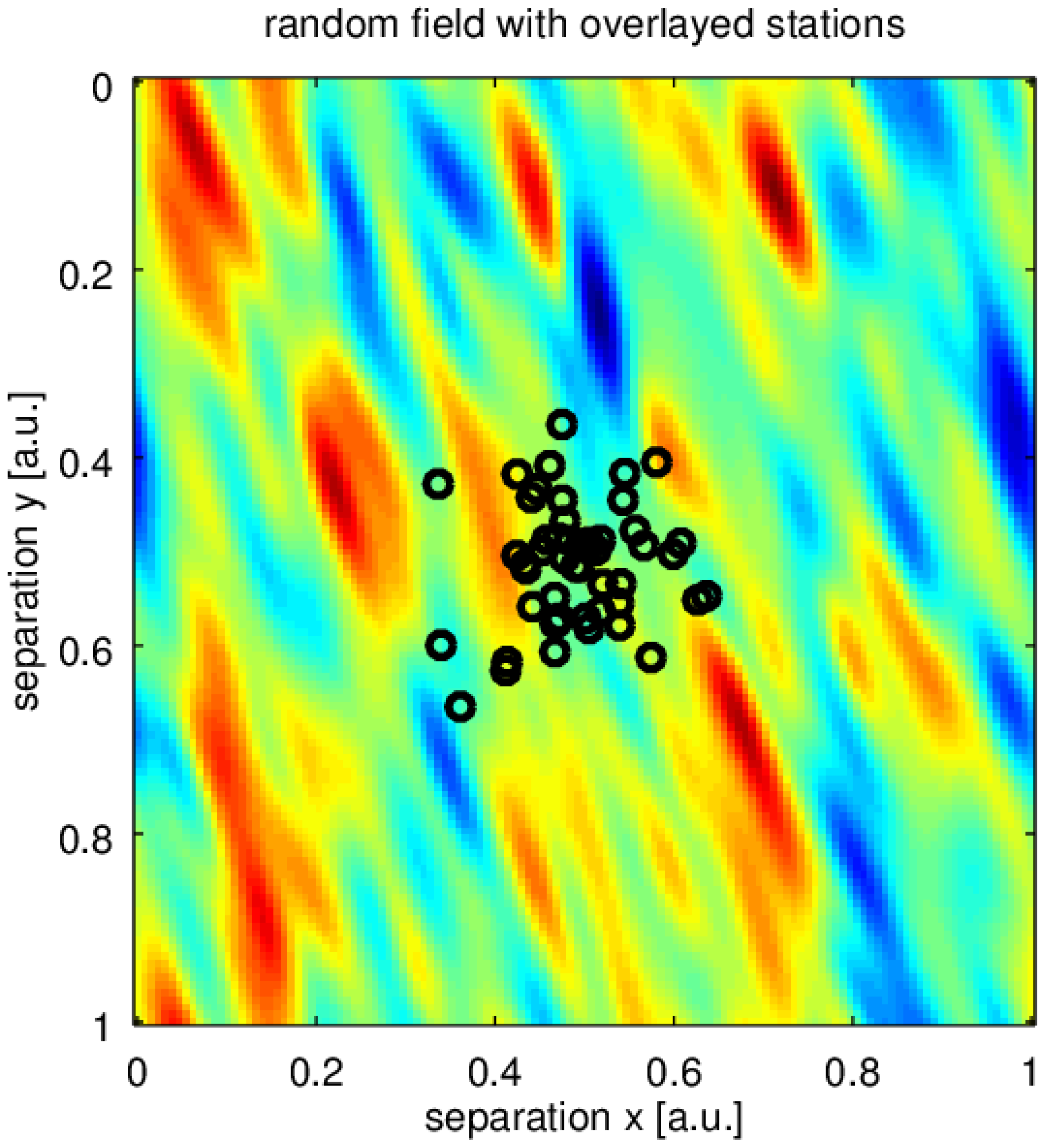
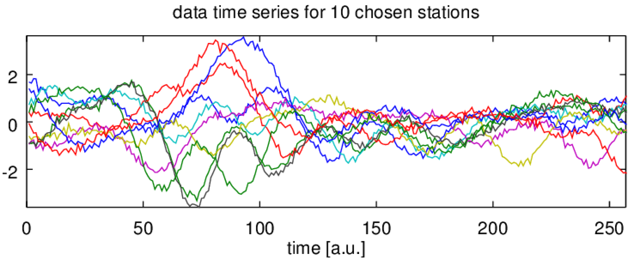
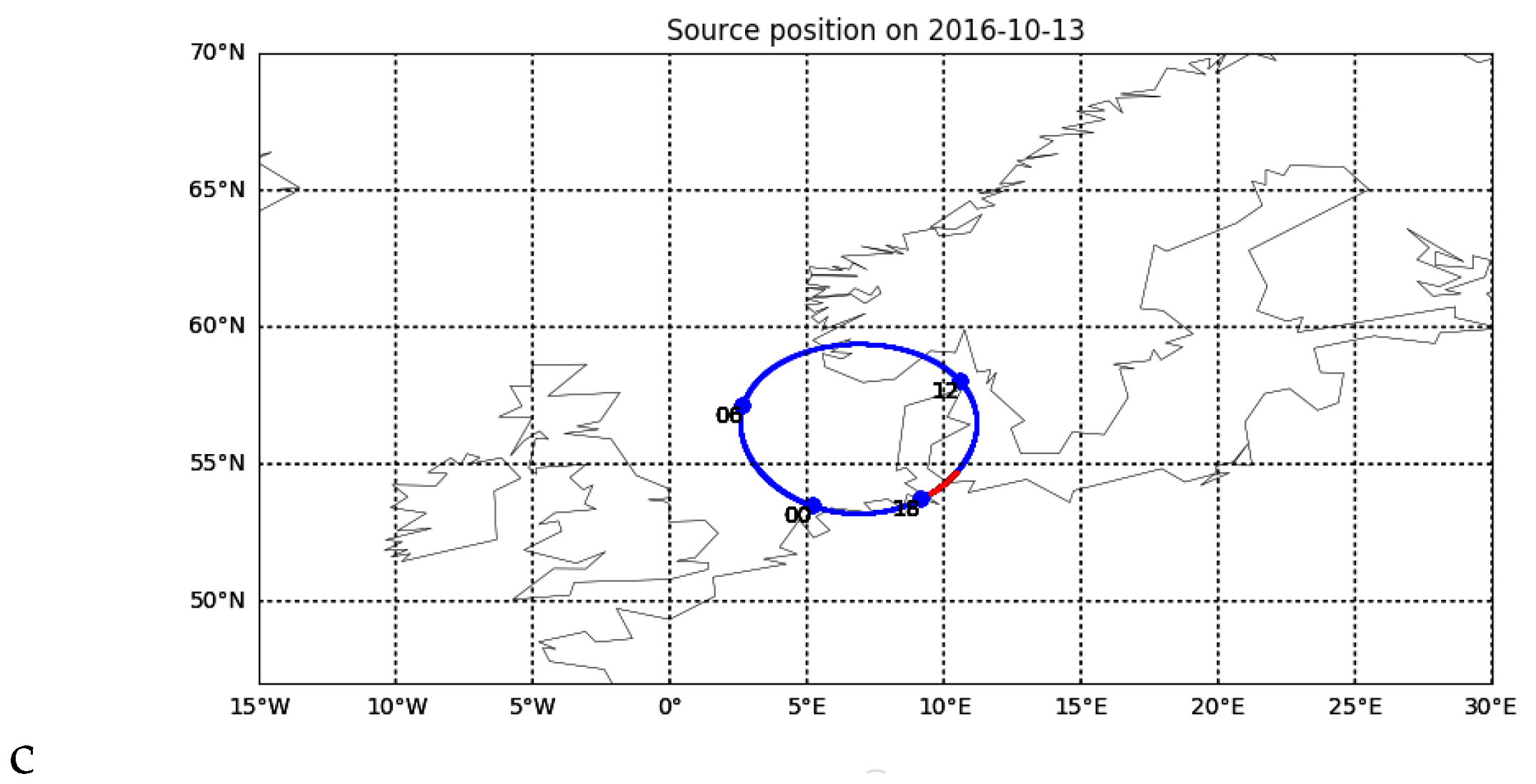
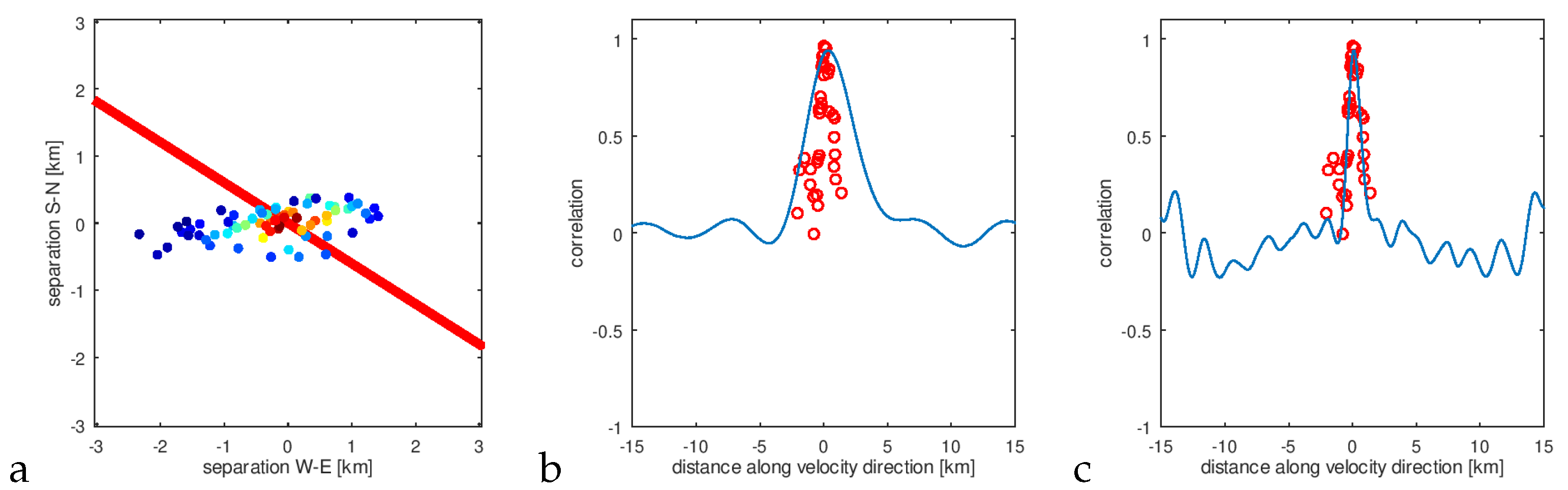
We present a simple numerical example illustrating described modelling. A set of virtual receiving stations (black circles in
Figure 2) samples a random field that is drifting past. An example of received signals is depicted in
Figure 3. Some mutual relations between each other can be observed. In
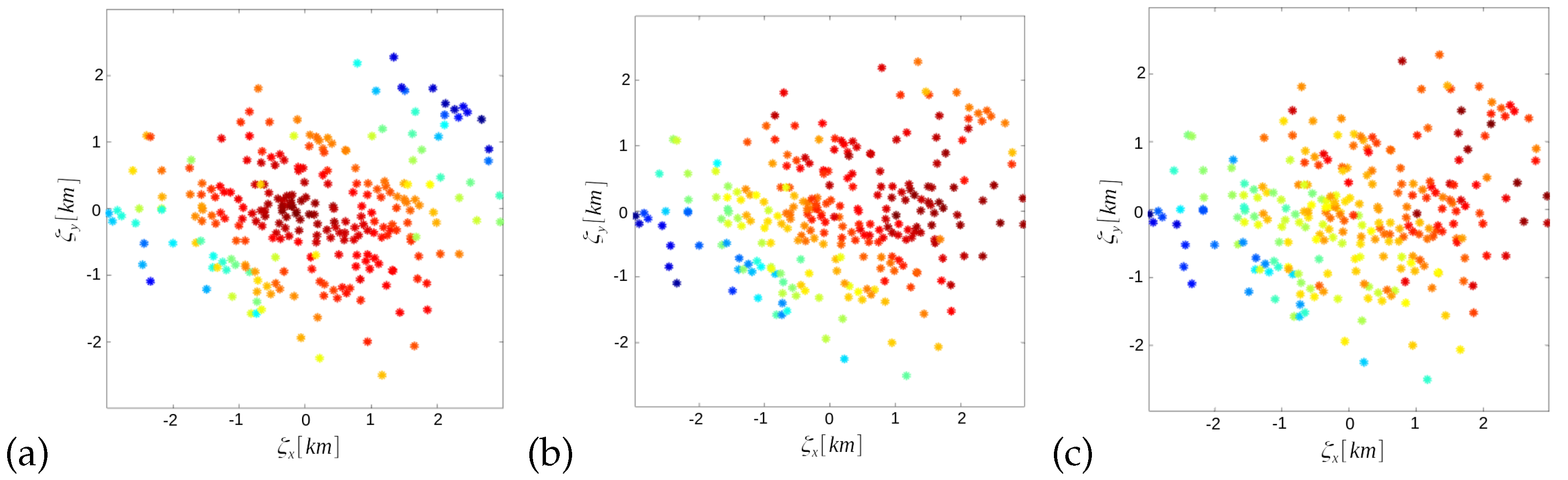
Figure 4a cross-correlations for each pair of signals for zero time lag have been plotted as a function of the separation vector. To assess matrix
Q we took least square fit of the function
to estimated correlations near
. Resulting ellipsis has been plotted at the same figure. Clearly, the correlation captures well basic spatial properties of the sampled field.
Figure 4b,c show time lag for maximum cross-correlation as a function of separation (it is clearly linear as formula (
9) predicts). Now, combining the information on structure geometry with time delay gradient, we were able to estimate drift velocity (red strip in
Figure 4c). The true drift velocity (black on
Figure 4b) is very close to the estimated (red on
Figure 4c). For comparison, we also give an isotropic estimate represented as the blue strip (the estimate of drift velocity obtained using the assumption of isotropy of random field—the quadratic form matrix is a scalar multiple of identity matrix in this case).
We will take an important note at this point. The above example shows that we reconstruct the spatio-temporal correlation for a given random field as:
As pointed out by Briggs in the exposition of his full correlation analysis [
6], the basic frozen flow drift estimation presented above can lead to serious overestimation of velocity magnitude in the presence of temporal decorrelation. When additional temporal decorrelation is present the evolution of a field can be described by a spatio-temporal quadratic form that takes the following form in the rest frame:
It also describes an elliptic shape of the isosurfaces of spatio-temporal correlation. The
is the spatial part of the full matrix, while
describes temporal fading. When the field is moving with the velocity v the matrix of the quadratic form transforms into:
, where T is the Galilean transformation to a new coordinate system moving with the velocity
:
Writing Q’ explicitly, it reads:
The important property of the Briggs model is that the correlation function depends on
and
through the same functional form
:
For this model we obtain the gradient of time lag to the maximum of cross-correlation:
For frozen flow and Briggs models, the gradient is linear, so this property cannot be used to discriminate them. The experimentally assessed quantities:
and
are the same, thus between the frozen flow velocity estimate
and
the scalar relation should hold:
where the scaling factor
gives the measure of overestimation of the drift velocity, when a pure frozen flow estimator is taken.
The relation (
17) provides another way of assessing the drift velocity:
Briggs model enables differences in functional dependence between spatial and temporal correlations [
6]; however, the simple form of dependence allows for the construction of relatively simple and practical algorithms for estimating the drift velocity [
12,
14]. In these algorithms, the arguments of the temporal cross-correlation functions for different positions are compared when the function values are equal. This leads to methods that are essentially similar to the Formula (
20). The same form of dependence for spatial and temporal changes facilitates the analysis and construction of practical algorithms, but lacks a solid physical foundation. This problem was discussed in the works of Little and Ekers [
15], where the authors considered the dispersion of structures motion, while Wernik et al. [
10] studied the importance of ionospheric propagation effects in the case of the vertical drift gradient in the scattering layer.
Data used for this analysis come from LOFAR core and remote station observations [
1]. The Low-Frequency Array (LOFAR) is an excellent astronomical instrument, and a handy tool for studying irregularities in the ionosphere [
1]. Due to its operational frequency range (10–270 MHz), LOFAR is very sensitive even to tiny changes in ionospheric electron density. The instrument’s interferometric nature allows for multi-point observations, thus giving the possibility for ionospheric scintillation measurements over distances ranging from tens of meters to hundreds of kilometres. The project for scintillation monitoring over the LOFAR stations has been carried out for several years, and a large amount of data has been collected and stored in the Long Term Archive (LTA,
https://lta.lofar.eu (accessed on 13 July 2022)). Available data contains signal amplitude for a few strongest radio sources measured at all core and remote stations in beam forming mode (not as an interferometer). Based on the LTA data, correlation analysis between stations can be done in order to obtain information about the characteristics of ionospheric structures.
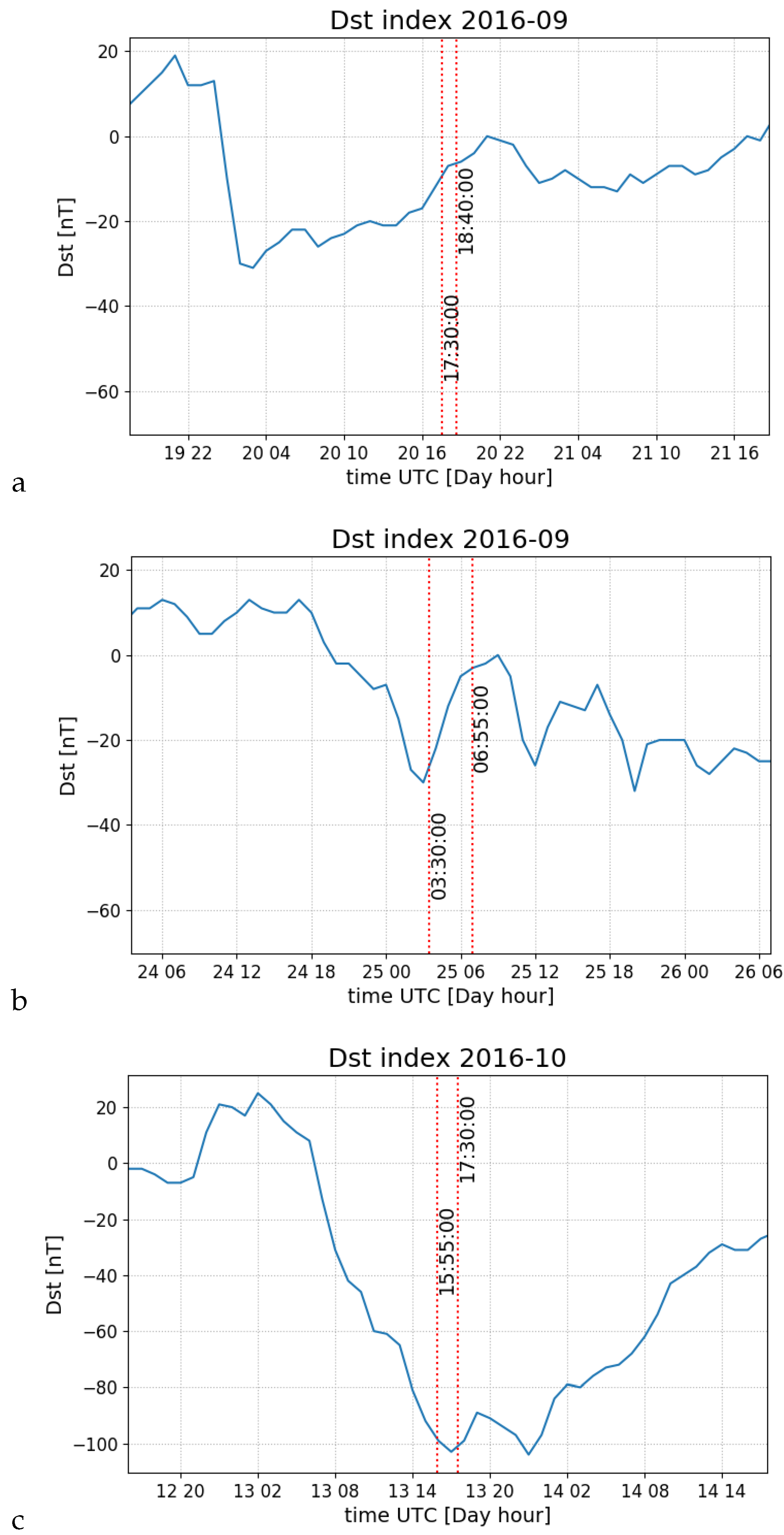
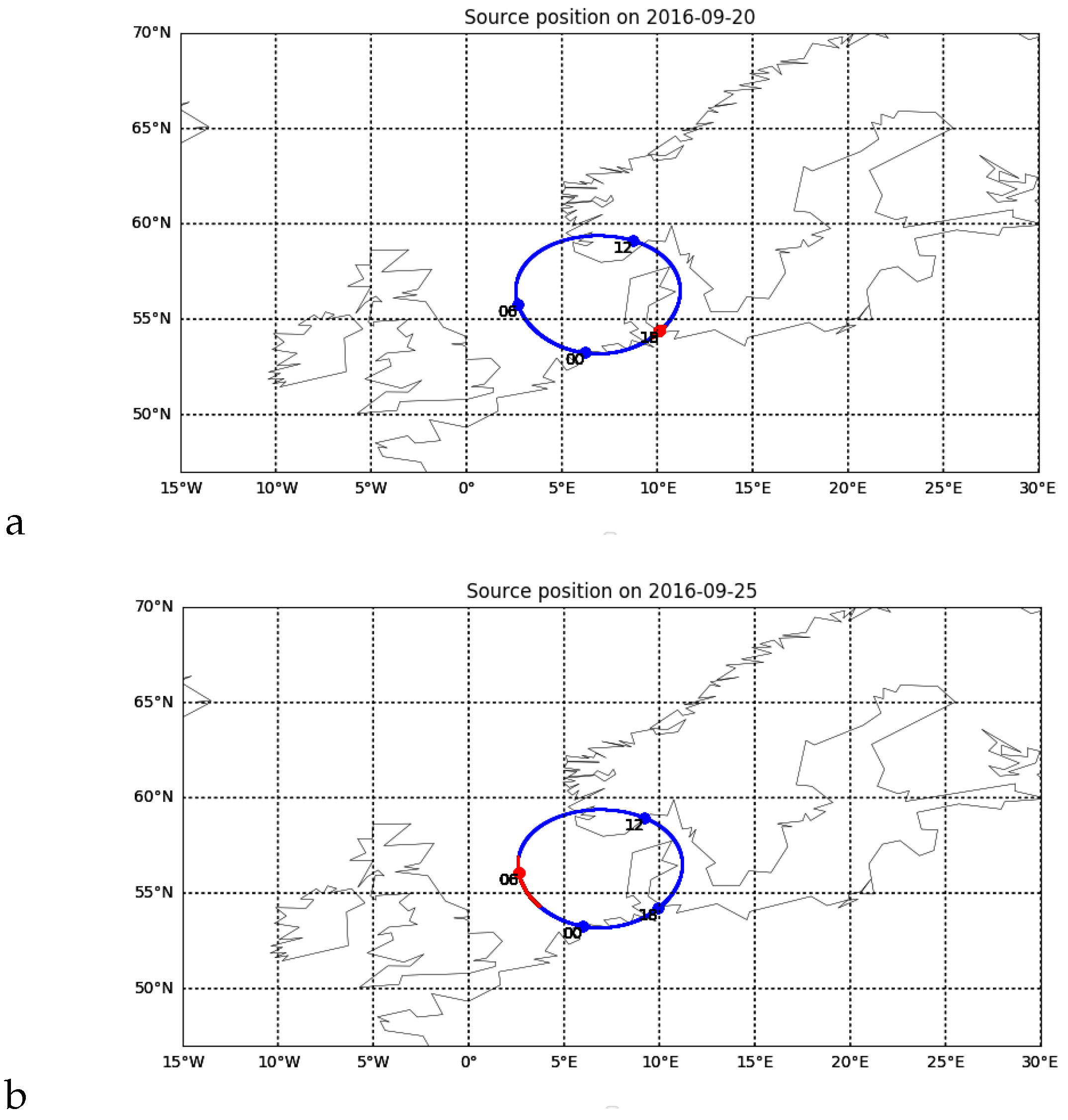
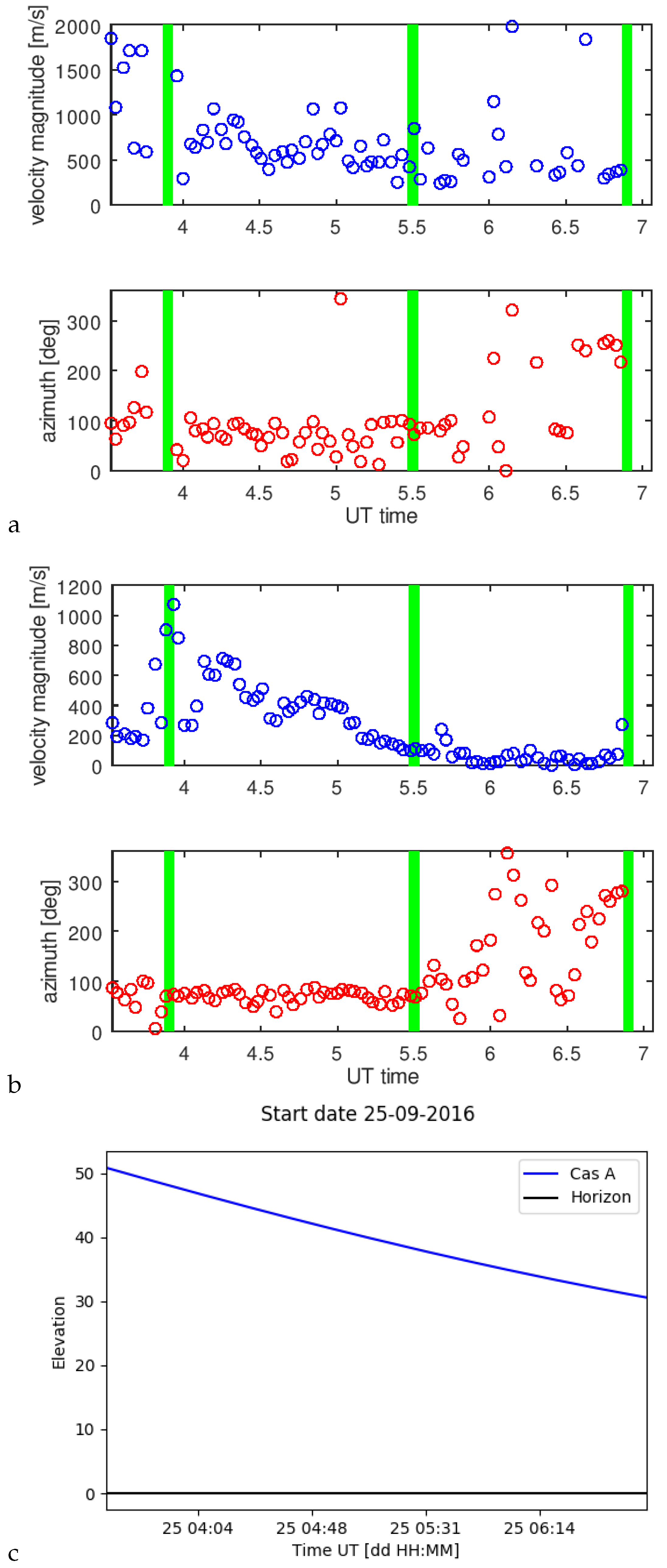
The Cassiopeia signal amplitude was observed under three various geomagnetic conditions (the key parameter describing geomagnetic conditions—Dst index, is shown in
Figure 5: a for L547449; b for L547785; c for L552177 set respectively). L547449 observations took place during the calm period, the L547785 is a phase of relaxation of a small geomagnetic disturbance, and L552177 was measured during the main phase of the magnetic storm (
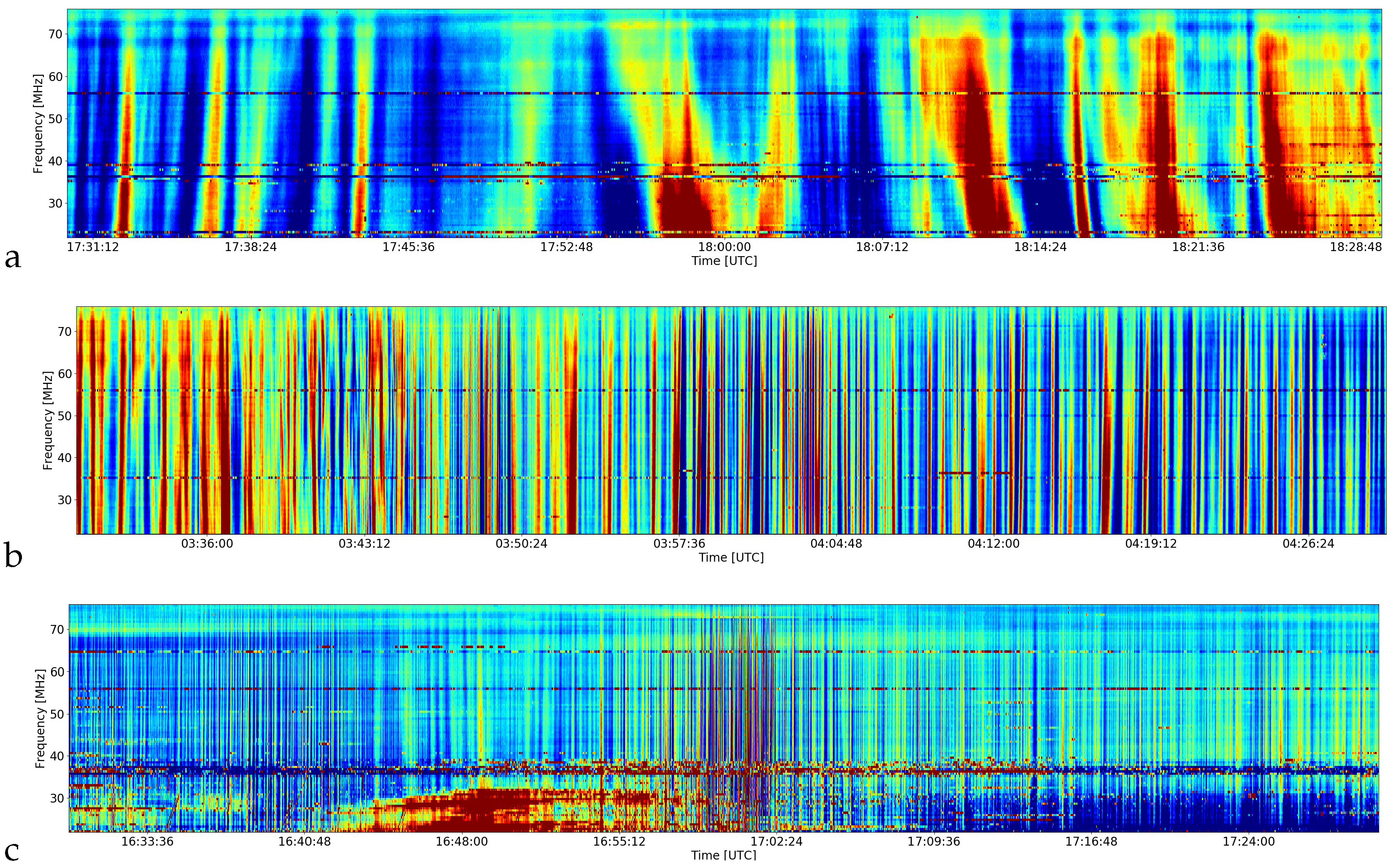
Table 1 gathers the details concerning the data sets). The amplitude dynamic spectra for these periods are shown on
Figure 6—one can see an increasing density of the structures observed which may be related to the increasing speed of ionospheric structures. Positions of ionospheric pierce points (IPPs) are shown as a red line pieces in
Figure 7 (IPPs were calculated at an altitude of 350 km).
3. Results
The Equation (
7) implies that the correlation function should satisfy the basic equation:
which describes the homogenous drift of the correlation function in the displacement coordinates.
Figure 8 illustrates such behaviour of the correlation function for the L547785 data set. One can see that the correlation function seems to be in movement (the plots show correlations for subsequent time instants).
The observed signals were analysed as described earlier in the numerical example.
Figure 9a,b,c show correlations for zero time shift as a function of stations position difference (the displacement coordinates) with the estimated quadratic form ellipse overlaid for different datasets, respectively. Geometry for all three cases seems to be well-defined, and their sizes do not depend on geomagnetic conditions.
Figure 9a1,b1,c1 show the time shift of the maximum cross-correlation as the function of the separation, the determined velocity vectors (red stripe) and the isotropic estimate, where
Q is a scalar multiple of the identity matrix, (blue strip). Black strip means vector speed with magnitude successively: 100 m/s, 1000 m/s, 1000 m/s for the reference. The exact results are gathered in
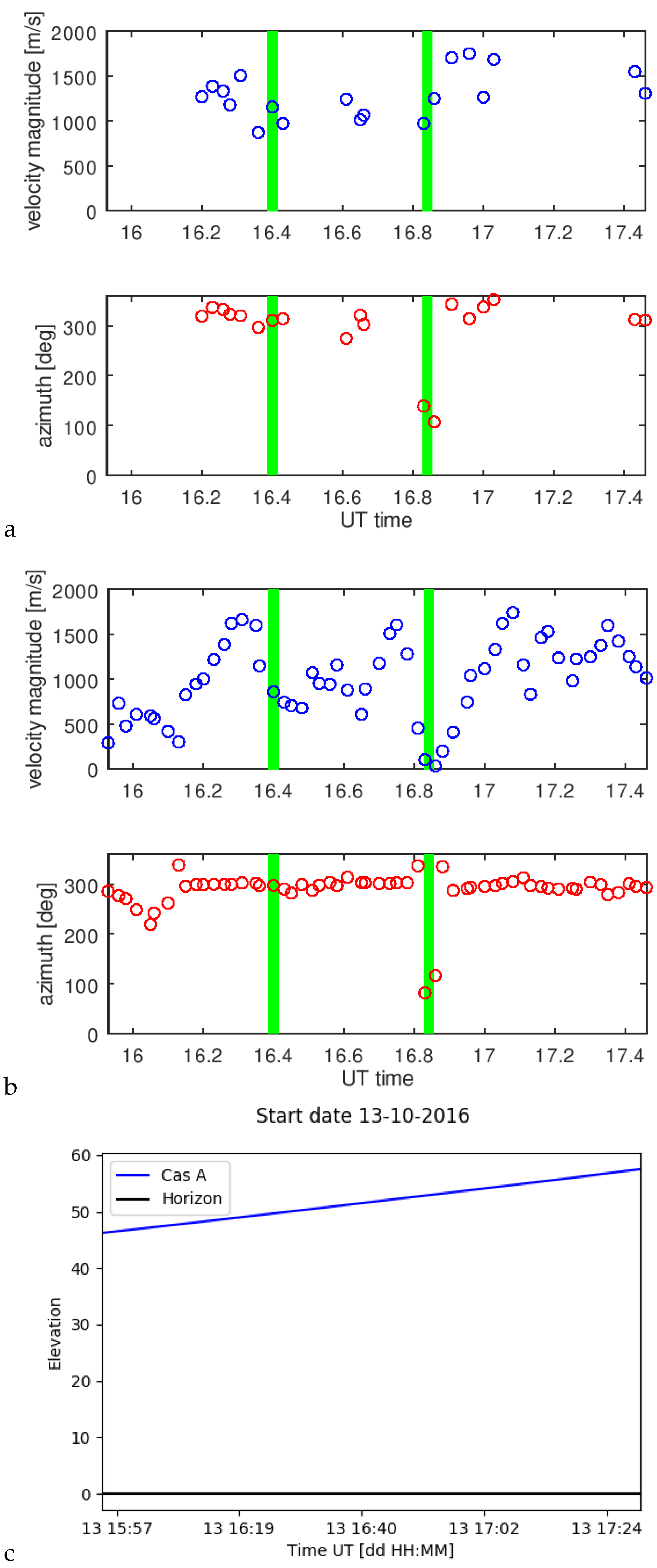
Table 2. One can observe the linear dependence of the time shift as a function of the separation vector.
The frozen drift values shown in the table seem to be overestimated, especially for disturbed conditions. It may result from non-stationarity. The conditions are changing during the time period or an incorrect model used for the estimation. To check this, we divided the fragments into shorter segments of 3.4 min (2048 points), overlapping by half their length. We also estimated
matrix to compute drift velocity according to the Formula (
20). In order to do so, for large correlation values of
around 0, we fit the polynomial of the second degree in three variables (
):
This allows calculating Q’ and the velocity
. The
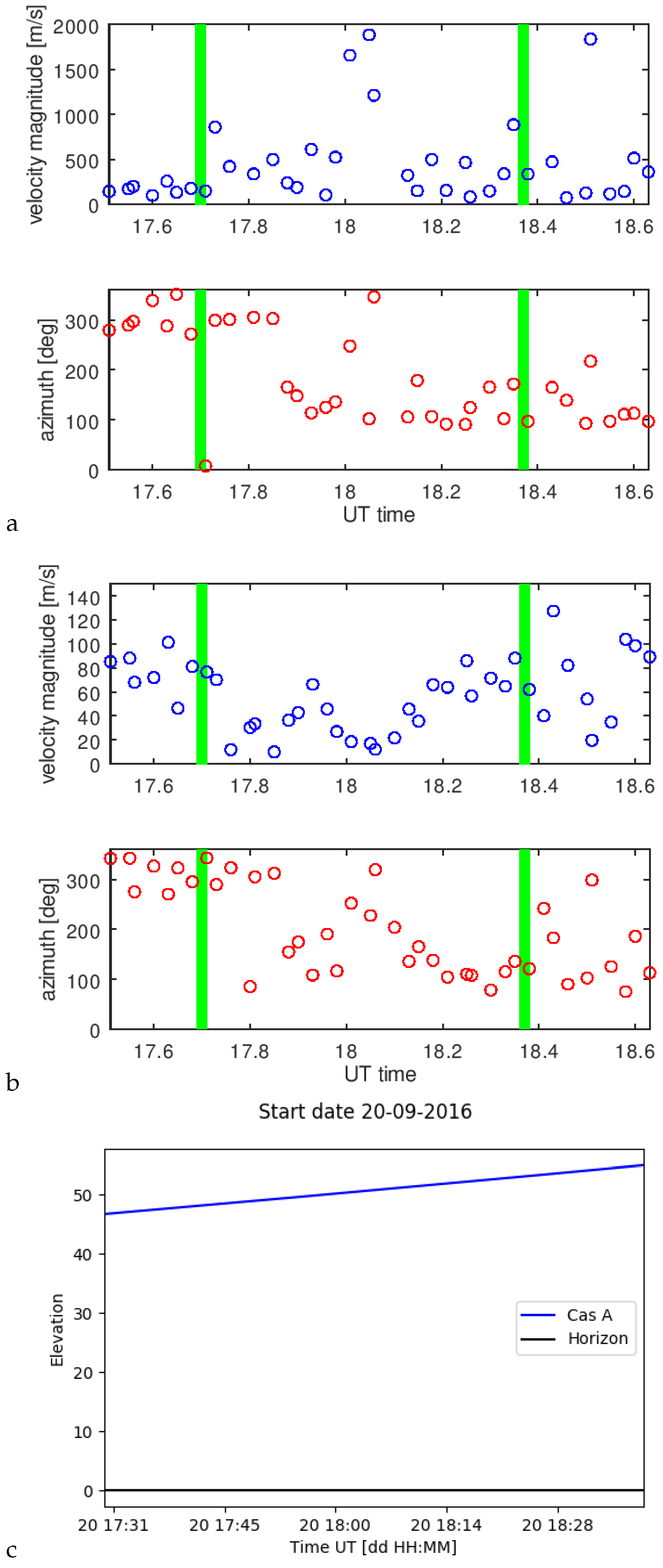
Figure 10,
Figure 11 and
Figure 12 show the results for both estimators and the source elevations for considered periods. In green, we marked the periods where we made the comparison with SuperDARN radar convection pattern assessments. We limited the plots to values less than 2000 m/s.
Having many pairs with a significant correlation at hand, it is possible to check the validity of the assumption of frozen drift. According to the Formula (
5), cross-correlation in the frozen flow case should be the intersection of the spatial correlation that goes through the separation vector for a given pair in the direction of the velocity vector. We constructed such an intersection by taking computed spatial correlations in a strip distant from the mentioned straight line no more than
d. We introduced spatial coordinates
for the temporal cross-correlation to compare the two quantities.
Figure 13 shows such a comparison for the selected data segment. One can see that the red points (spatial correlations) do not lie on the blue line showing temporal cross-correlation between two stations. As we pointed out, the frozen drift assumption can lead to overestimating the drift velocity. We tried to determine the factor by which
should be multiplied so that the curves overlap. For this purpose we minimise the following quantity:
with respect to
, where
gives the experimental velocity scaling factor. We also have given the velocity scaling factor for Briggs model (
20)
, which we can get from quadratic form
:
At this point we used the estimate (
20) of the drift velocity that - in the Briggs model - should be consistent with (
24).
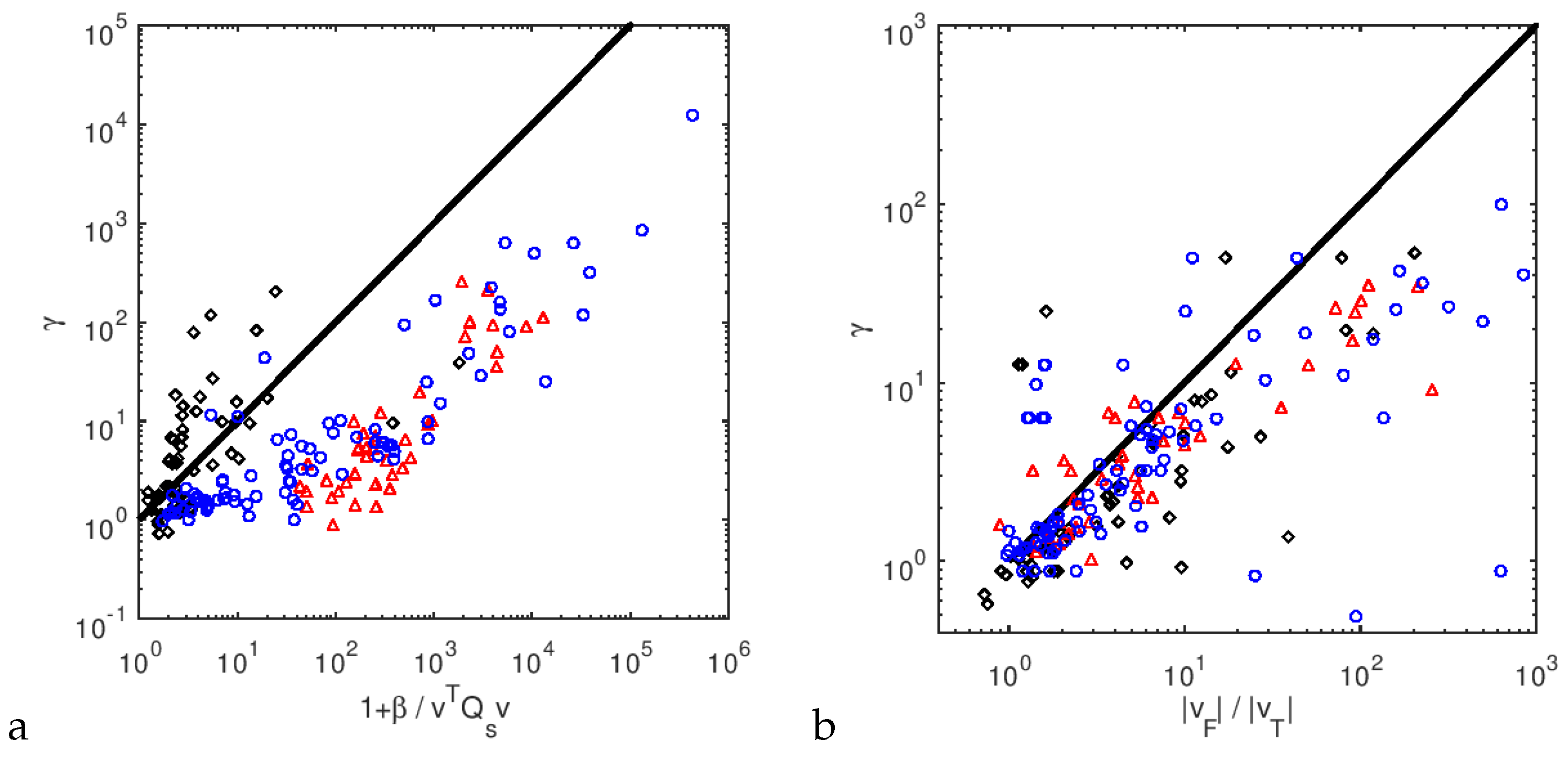
Figure 11a shows experimental velocity scaling factor
vs.
(
20) given by Briggs model. The different markers refer to different data sets: black diamonds—L552177; blue circles—L547785; red triangles—L547449. One can see a quite large discrepancy between the theoretical scaling and experimental one, moreover, the markers representing different data sets are distributed nonuniformly. For a comparison
Figure 11a gives experimental velocity scaling factor
vs. the ratio of velocity estimators magnitude
. In the latter case, one can see that the velocity modulus quotient is much closer to the experimental scaling factor than the theoretical value, and the points corresponding to the different data sets are evenly distributed. In
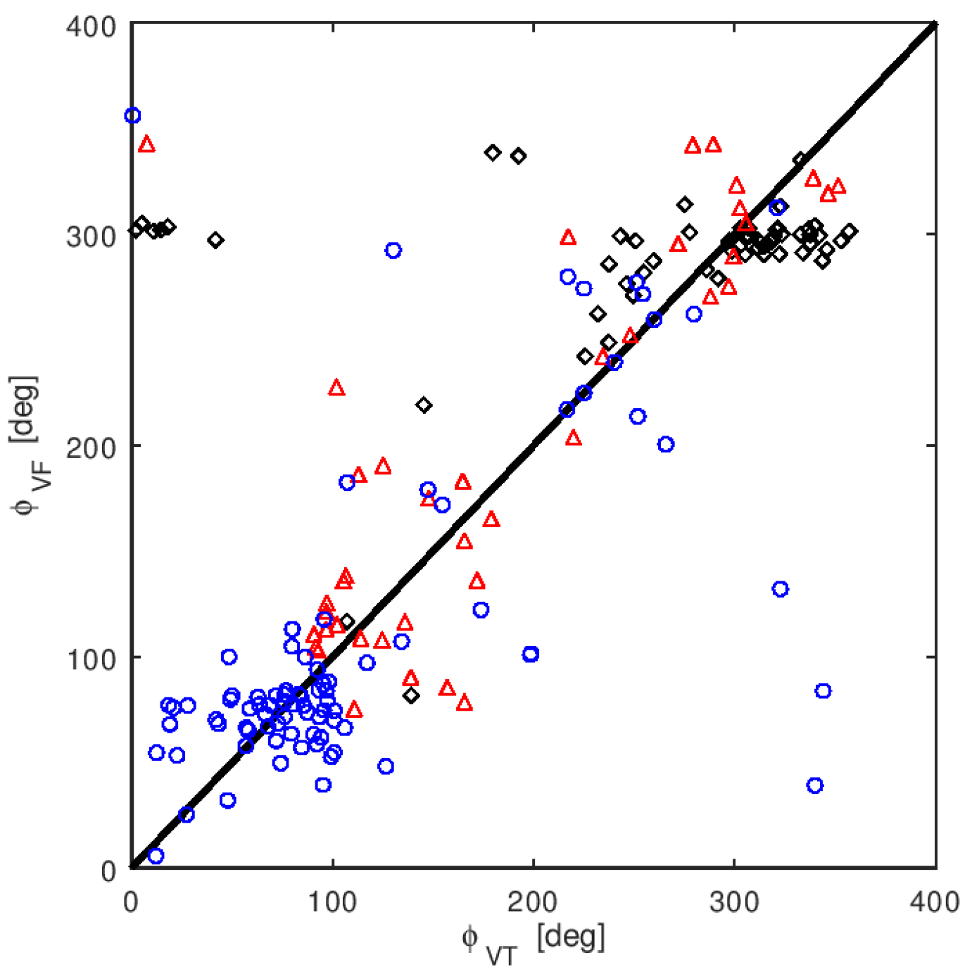
Figure 12 the relation between azimuths of
and
is shown. They roughly agree, however a minority has large deviations, which may suggest that the relation between estimates is not scalar. The points grouping suggests that estimates have mainly zonal component, which is in agreement with the SuperDARN observations (
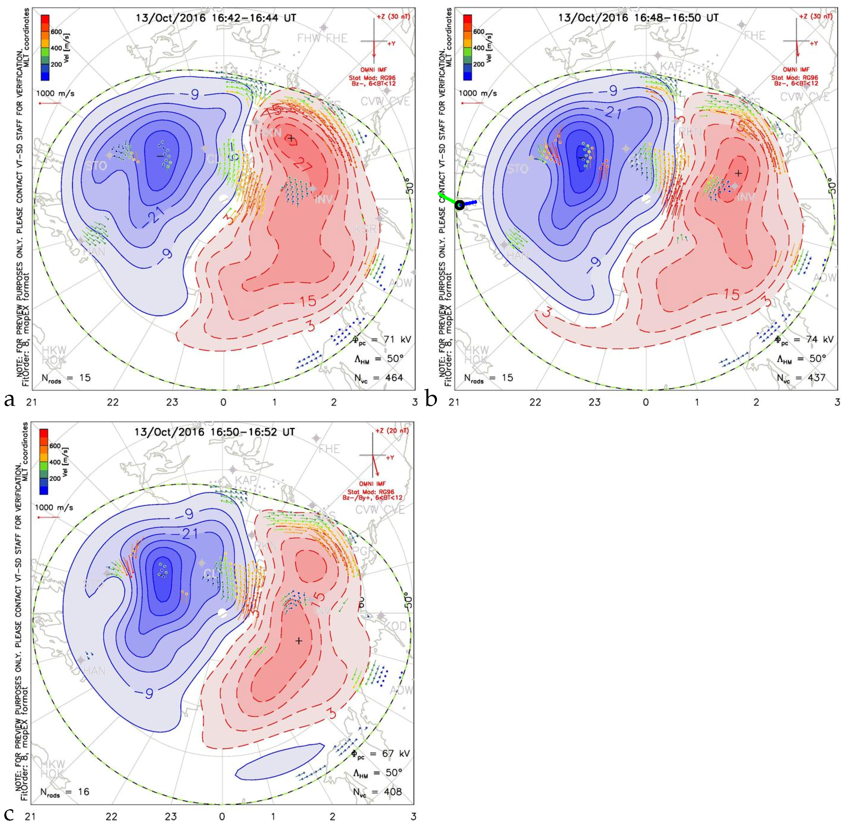
Figure 14,
Figure 15,
Figure 16 and
Figure 17).
We also present a comparison of the obtained results with the velocity estimates that use other experimental principles. For comparison, we will use the available plots showing the convection of the northern polar ionosphere modelled on the basis of measurements by the SuperDARN system [
16].
Figure 14,
Figure 15,
Figure 16 and
Figure 17 show the velocities overlayed on the ionospheric convection maps given by SuperDARN system around the moments of time marked with green lines in
Figure 10,
Figure 11,
Figure 12,
Figure 13,
Figure 14,
Figure 15,
Figure 16,
Figure 17,
Figure 18 and
Figure 19 respectively. The green colour strip gives the frozen flow estimate
while the blue one the
. We keep exact mutual relation between estimates while abandoning accurate comparison to the SuperDARN drift velocity magnitudes. The reason is twofold: we would like to highlight our results that otherwise would be obscured if given in scale. The second reason is that the location of our estimates is outside of the validity of SuperDARN modelling yet still close enough to bear some features of large-scale polar ionosphere convection. Inevitably, the comparison is qualitative for the reasons we mentioned, but they can be used to trace possible drift at mid-geomagnetic latitudes.
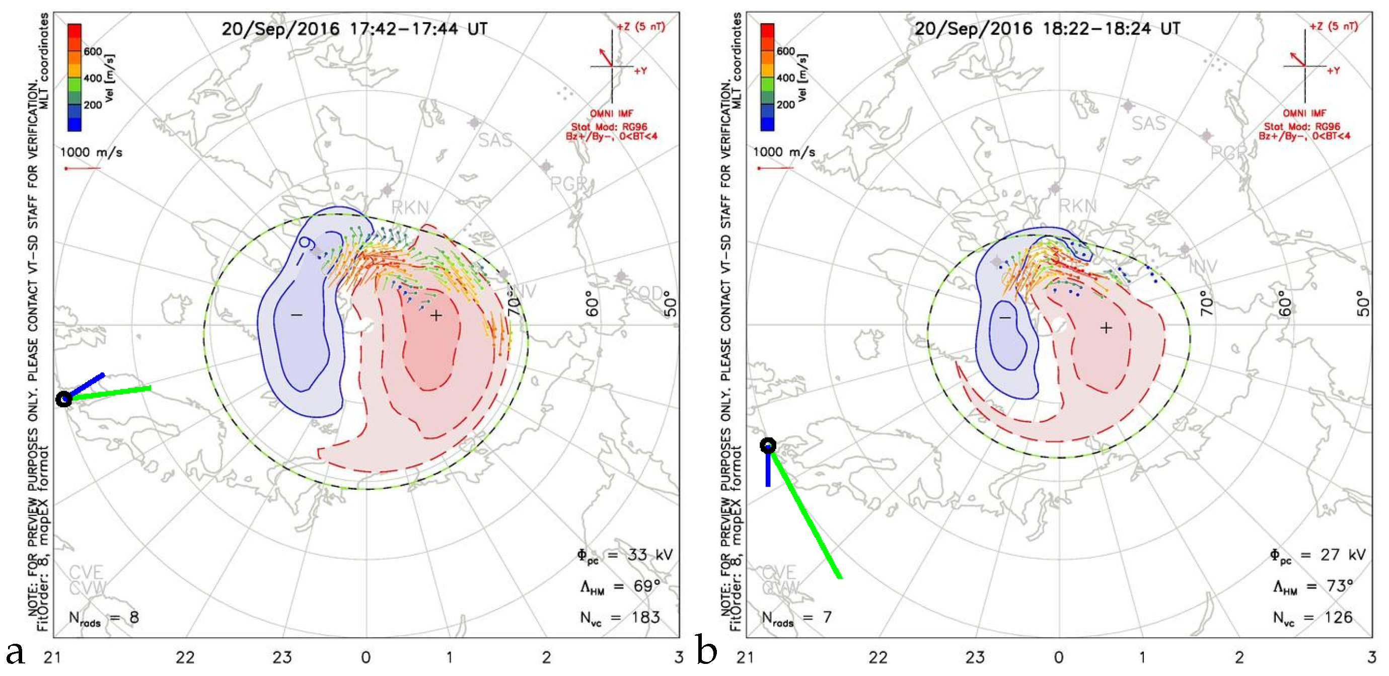
Figure 14 shows that for chosen time instants of the L547449 data set our estimates agree with distant polar convection at least around 18:22 UT. Similarly,
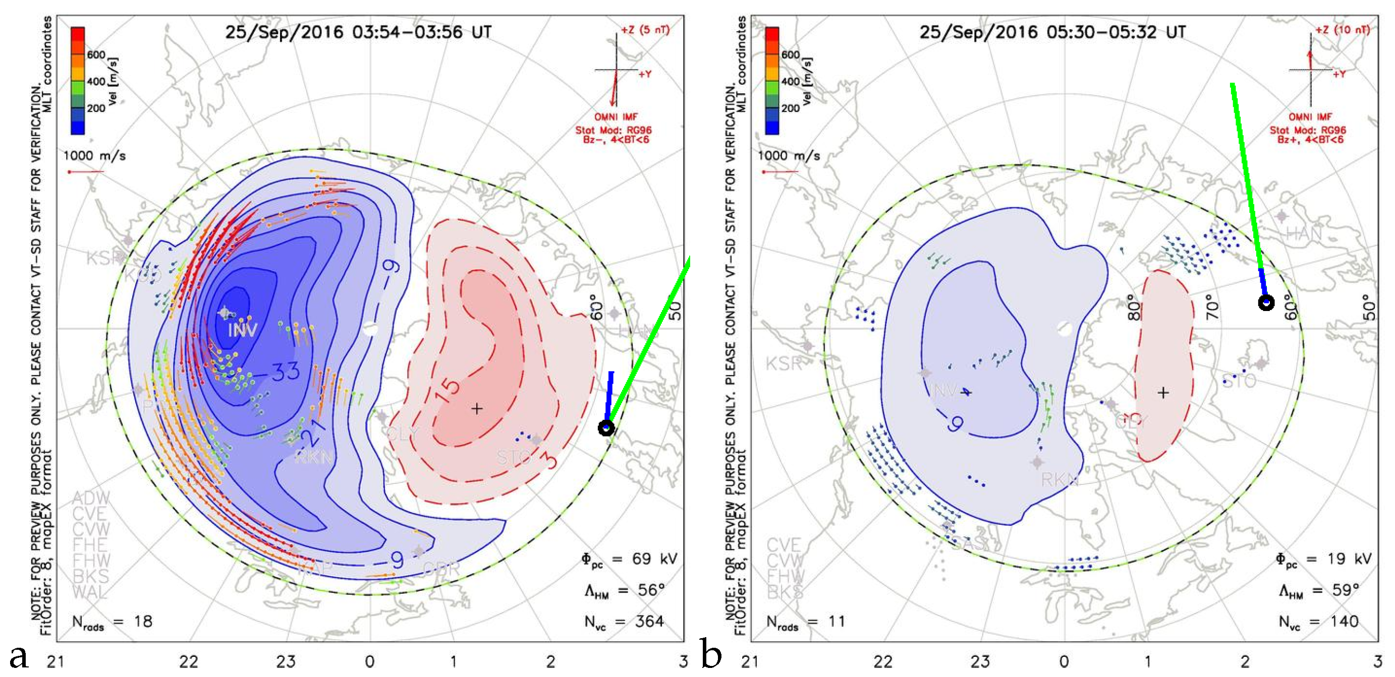
Figure 15 shows an agreement of our estimates with the polar ionosphere convection for the L547785 data set and
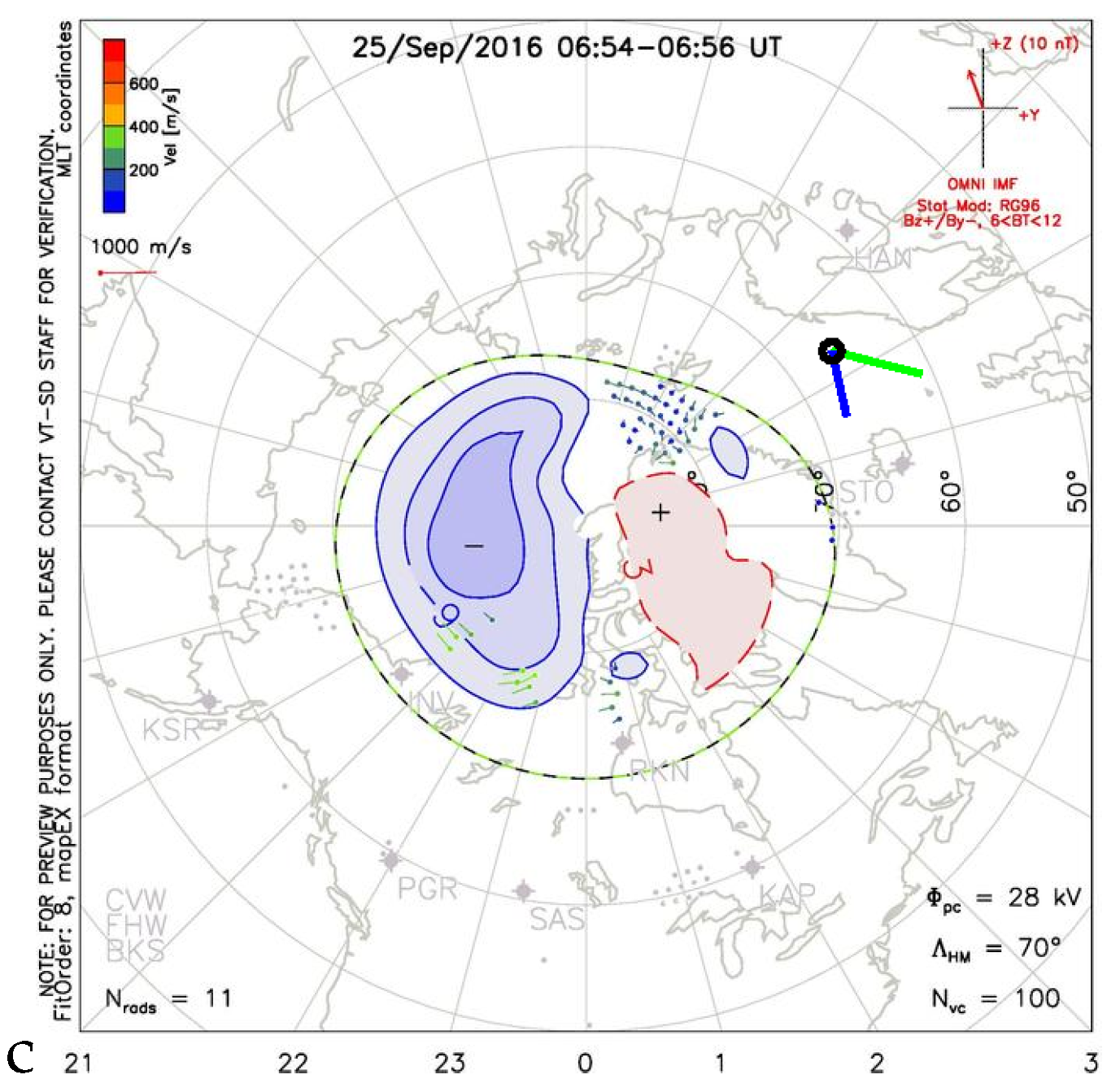
Figure 16 for L552177.
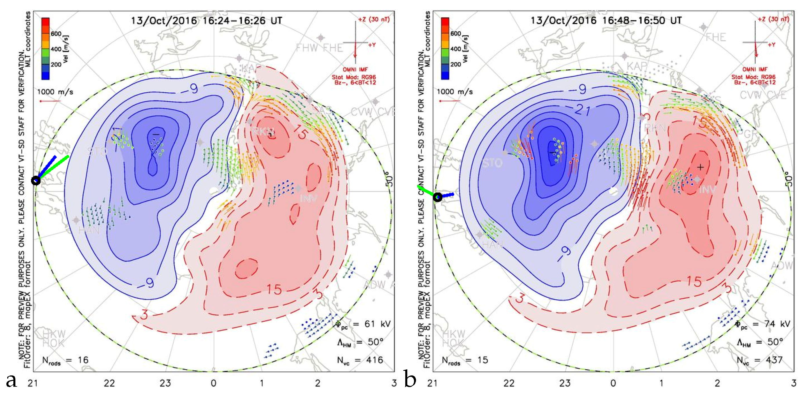
Figure 17 shows signatures of reaching a flow stagnation point around 16:45 UT. Here, additionally, we display SuperDARN convection assessment before and after the event. A tongue of eastward circulation reaches far west.
Although the estimates of the ionospheric drift velocity follow the convection pattern assessed by SuperDARN system for mid-latitude ionosphere may seem exaggerated for sets L547785 and L552177. To illustrate, that such values are still possible we present the drift estimations made by the ionosphere soundings at Pruhonice (49°59′N 14°32′E), Juliusruh (54°37′N 13°22′E) and Fairford (51°41′N 1°46′W) during the storm of 13.10.2016 which are respectively: 976 +/− 130 m/s (at 16:49 UT), 405 +/− 18 m/s (at 17:15 UT), 833 +/−146 m/s (at 17:53 UT) (
https://giro.uml.edu/driftbase/ (accessed on 13 July 2022)). This illustrates possible ionospheric variability in space and time during disturbed conditions at mid-latitudes.


 ,
, 


