Automated Road-Marking Segmentation via a Multiscale Attention-Based Dilated Convolutional Neural Network Using the Road Marking Dataset

Abstract

Road markings, including road lanes and symbolic road markings, can convey abundant guidance information to autonomous driving cars. However, recent works have paid less attention to the recognition of symbolic road markings compared with road lanes. In this study, a road-marking-segmentation dataset named the RMD (Road Marking Dataset) is introduced to compensate for the lack of datasets and the limitations of the existing datasets. Furthermore, we propose a novel multiscale attention-based dilated convolutional neural network (MSA-DCNN) to tackle the proposed RMD. The proposed method employs multiscale attention to merge the weighting outputs of adjacent multiscale inputs, and dilated convolution to capture spatial-context information. The performance analysis shows that the proposed MSA-DCNN yields the best results by combining multiscale attention and dilated convolution. Additionally, the proposed method gains the mIoU of 74.88%, which is a significant improvement over the existing techniques.

1. Introduction

In recent years, autonomous-driving approaches and advanced driver assistance systems (ADASs) have resulted in unprecedented development at both the academic and industrial levels [1]. The breakthroughs in the fields of deep learning and computer vision, as well as the tremendous computational ability of graphics processing units (GPUs), open the door to research on fully autonomous driving. Fully autonomous driving requires traffic-scene understanding, including traffic-sign recognition, vehicle and pedestrian detection, and road-surface recognition (e.g., road-marking recognition) [2,3]. Lane detection, which is a task of road-surface recognition, plays a vital role in autonomous driving, as road lanes demonstrate the drivable area on the road for vehicles [4]. In the field of lane detection, a variety of methods have been proposed, comprising traditional handcrafted feature-based methods and convolutional neural network (CNN)-based methods [5,6,7,8,9,10,11,12].

However, on urban roads, where autonomous driving faces complex and diverse problems, lane detection is not the only component of road-surface recognition. In addition to the drivable area imposed by road lanes, there is abundant information that can assist the drivers provided by symbolic road markings on road surfaces. Road markings, including road lanes and symbolic road markings, refer to the application of paints on road surfaces to communicate information to drivers and pedestrians, as shown in Figure 1. Generally, a standard system of road markings can convey drivable areas, directions, speed limits, stopping, etc. [13]. It is commonly believed that understanding the abundant guidance information provided by symbolic road markings increases the safety of autonomous driving. However, the publicly available datasets of and approaches to road-marking recognition pay less attention to the recognition of symbolic road markings than road lanes [14].

Several commonly used and publicly available datasets have been released to evaluate various algorithms in the field of autonomous driving (e.g., the KITTI Vision Benchmark Suite (KITTI) [15], Cityscape Dataset (Cityscape) [16], Mapillary Vistas Dataset (Mapillary) [17], Cambridge-driving Labeled Video Database (CamVid) [18], BDD100K [19], TuSimple Benchmark Dataset (TuSimple) [20], and CurveLanes Dataset [21]). However, most of the datasets mentioned above only contain a road lane, and some of them include limited types of road markings. These limitations mean that road-marking recognition is sometimes difficult [13]. For the perception of road markings, Road Marking Detection [22] was the first publicly available dataset, released in 2013, and it consists of 1443 labeled images with bounding-box annotation belonging to 11 symbolic road-marking classes. Most of the earlier works [23,24] using handcrafted feature-based methods are evaluated on the Road Marking Detection dataset. However, there exists the problem that multiple images present the same scene in Road Marking Detection (e.g., from the image of roadmark_1202 to the image of roadmark_ 1259). VPGNet [25] and TRoM [14] have become the most popular datasets in road-marking recognition since 2017. VPGNet contains 21,097 labeled images with pixel-level annotation belonging to 17 classes, while TRoM contains 712 labeled images with pixel-level annotation belonging to 19 classes. Recent works [13,25,26,27] based on CNN methods have addressed the problem of road-marking segmentation using VPGNet and TRoM. However, it has been indicated that the instance frequency of the symbolic-road-marking classes is much lower than that of the road lanes in VPGNet and TRoM [28]. CeyMo [28] is a new dataset for road-marking detection consisting of 2887 labeled images belonging to 11 road-marking classes (released in 2022). Although CeyMo makes up for the shortcoming of the low frequency of instances for symbolic road markings, the number of classes of road markings is too small compared with the real-world situation.

As described before, research on road-marking perception remains an ongoing challenge due to the lack of datasets and the limitations of the existing datasets. Hence, a new dataset called the Road Marking Dataset (RMD) was created to cope with the real-world conditions of urban road markings in this study. The RMD has 3221 well-labeled images belonging to 30 classes that were collected from three cities in Japan (i.e., Yokohama, Chofu, and Nogata). The RMD covers 29 categories of road markings on urban road surfaces, and it has the largest number of classes among the existing datasets.

The RMD contains both road lanes and symbolic road markings. This study focuses on road-marking segmentation. Hence, a multiscale attention-based dilated convolutional neural network (MSA-DCNN) is proposed and applied to the RMD. The proposed MSA-DCNN takes multiple-scale images that are resized from the original image as inputs to learn the attention weights of each scale, following merging the semantic predictions to obtain the final output. In addition, dilated convolution [29] is adopted in the feature-extraction process to utilize a larger range of spatial-context information. The main inspiration of the proposed method comes from previous studies [30,31]. Chen et al. [30] resize the input images to several scales to pass them through a shared network, and they prove that multiscale inputs improve the performance of semantic segmentation compared with a single-scale input. The experiments in [31] show that large-scale objects can be better segmented in resized images with reduced pixel counts because the receptive field of the CNN can observe more global context. Moreover, fine details, such as objects of thin structures, can be well predicted in resized images with increased pixel counts.

The remainder of this paper is organized as follows. Section 2 describes the related work. Section 3 introduces the proposed dataset. Thereafter, the proposed method is presented in Section 4. Section 5 presents the results of the experiments. Finally, Section 6 concludes the paper.

2. Related Work

2.1. Road-Marking Recognition

The earlier works [4,23,32,33] on road-marking recognition commonly adopted a combination of highly specialized handcrafted features and heuristics to identify road markings [1]. The common procedure of the traditional methods is distortion correction, inverse perspective mapping (IPM), feature extraction, and line or curve fitting. Within the last few years, the research into deep learning and computer vision has witnessed exciting progress, which has been expanded into autonomous driving and ADAS applications. It has been shown that CNN-based methods outperform traditional approaches in many applications [12]. Therefore, CNN-based methods have been replacing handcrafted feature-based methods in road-marking recognition. Davy et al. [1] proposed an end-to-end solution to lane detection for the first time by converting lane detection to an instance-segmentation problem. Pan et al. [3] won first place on TuSimple [20] by proposing a spatial convolutional neural network (SCNN) in 2017 in which traditional layer-by-layer convolutions are converted to slice-by-slice convolutions within feature maps. The aforementioned lane-detection approaches adopted the idea of segmentation, finding all the masks belonging to the same road lane, and then outputting the lane line through the method of curve fitting.

For the recognition of symbolic road markings, Lee et al. [25] exploited vanishing-point prediction to guide robust lane and road-marking detection. Liu et al. [13] presented the residual neural network (ResNet) [34] with pyramid pooling (RPP) as the baseline model for their TRoM dataset. Oshada et al. [28] presented two baseline models, an object-detection model and an instance-segmentation model, as baseline models for their CeyMo dataset. As mentioned in Section 1, the approaches to road-marking recognition pay less attention to the perception of symbolic road markings than road lanes. Although algorithms on road-lane detection [1,3,11] have achieved convincing results, CNN-based methods on symbolic road markings have rarely been seen, except in [14,25,28].

2.2. Semantic Segmentation by CNN

Semantic segmentation is a computer-vision task that associates a class with each pixel of an image. It is used to identify the cluster of pixels that make up a distinguishable class. Various methods [29,35,36,37,38] have been proposed to address problems on different topics, such as the semantic segmentation of medical images, satellite images, street views, etc. Most of the current mainstream semantic-segmentation methods are based on a work called the fully convolutional network (FCN) for semantic segmentation [35]. Different from the classic CNN that uses the fully connected layer after the convolutional layers to obtain a fixed-length feature vector for classification, the FCN uses the deconvolution layer to upsample the feature map to the same size as the input image. However, FCN-based methods usually have the problem that the gradually decreasing feature-map resolution will lead to the loss of spatial information as the network deepens. U-Net [36] is assuredly one of the most successful methods, and particularly in the task of medical-image segmentation. The encoder–decoder structure and skip connections are still the core ideas of many CNN-based methods that ensure that the feature map of each layer in the decoder part is fused by low-level features and high-level features. The pyramid scene-parsing network (PSPNet) [38] obtained high-quality results in scene-parsing tasks by introducing context information to the network. The PSPNet employs the feature extraction layers of ResNet-101 [34] for the encoder, and it adds a pyramid pooling module (PPM) between the encoder and decoder to gather spatial-context information. The encoder part of DeepLabv3+ [29] adopts a CNN with atrous convolution, in which ResNet [34] can be used, following atrous spatial pyramid pooling (ASPP), which mainly utilizes multiscale context information. The decoder part further fuses low-level features with high-level features to improve the accuracy of the segmentation boundaries [29,37].

2.3. Multiscale Context

The problem of multiple-scale objects is prevalent in the proposed RMD. Due to the size and location of road markings, the pixels occupied by each instance are different. As shown in Figure 1e, the number of pixels occupied by the road marking of maximum speed limit 40 on the left side of the road is significantly greater than that on the right side of the road, although they are the same object. Chen et al. [29] specify this problem as the existence of objects at multiple scales, which is a main difficulty for the task of semantic segmentation. To handle the problem, a wide range of methods have been proposed [30,36,37,38], which can be summarized into the following four types of network architectures, shown in Figure 2 [29].

The first type is the image pyramid (Figure 2a), which uses images of different sizes as inputs to obtain individual predictions by two separate networks. The final output is commonly derived by merging the two predictions by average pooling or max pooling [30]. U-Net [36], which adopts an encoder–decoder structure, is a typical example of the second type (Figure 2b). The encoder–decoder structure extracts multiscale features from the encoder part, and it restores the feature-map resolution by the decoder part. The third type (e.g., the DeepLab series [29,37]) employs dilated convolution (atrous convolution) using different dilation rates to extract multiscale features (Figure 2c). Furthermore, dilated convolution can control the receptive field of the feature map. The fourth type is spatial pyramid pooling (SPP) (e.g., PPM of the PSPNet [38]), which can accept a feature map of any size, and then control the size of the feature map after SPP (Figure 2d).

3. Proposed Dataset

The proposed RMD is a new dataset for the semantic segmentation of road markings, including symbolic road markings and road lanes. It comprises 3221 pixel-level annotated road-surface images of 29 road-marking categories, with a size of 1920 × 1080. The RMD was built with the aim of making up for the lack of datasets and the limitations of the existing datasets in the field of road-marking recognition, as mentioned in Section 1. The raw data of the proposed RMD were collected by a camera mounted inside a vehicle from three cities in Japan: Yokohama, Chofu, and Nogata, in November 2015, November 2015, and March 2017, respectively. Thereafter, from the 9779 frames of road-surface scenes obtained, 3221 representative scenes with more than one symbolic road marking were extracted for composing the RMD, which ensured that each image contained at least one symbolic road marking.

As shown in Figure 1, a variety of scenarios, such as (a) ordinary, (b) shadow, (c) dazzle light, (d) occlusion, (e) deteriorated road markings, and (f) narrow road, were carefully selected to design the proposed RMD. To the best of our knowledge, the RMD covers the most categories compared with the other existing datasets, as shown in

Table 1. Comparative statistics of the proposed RMD with the existing datasets.

Dataset	Categories	Images	Location
Road Marking Detection [22]	11	1443	USA
VPGNet [25]	17	21,097	Korea
TRoM [14]	19	712	China
CeyMo [28]	11	2887	Sri Lanka
RMD (this study)	30	3221	Japan

.

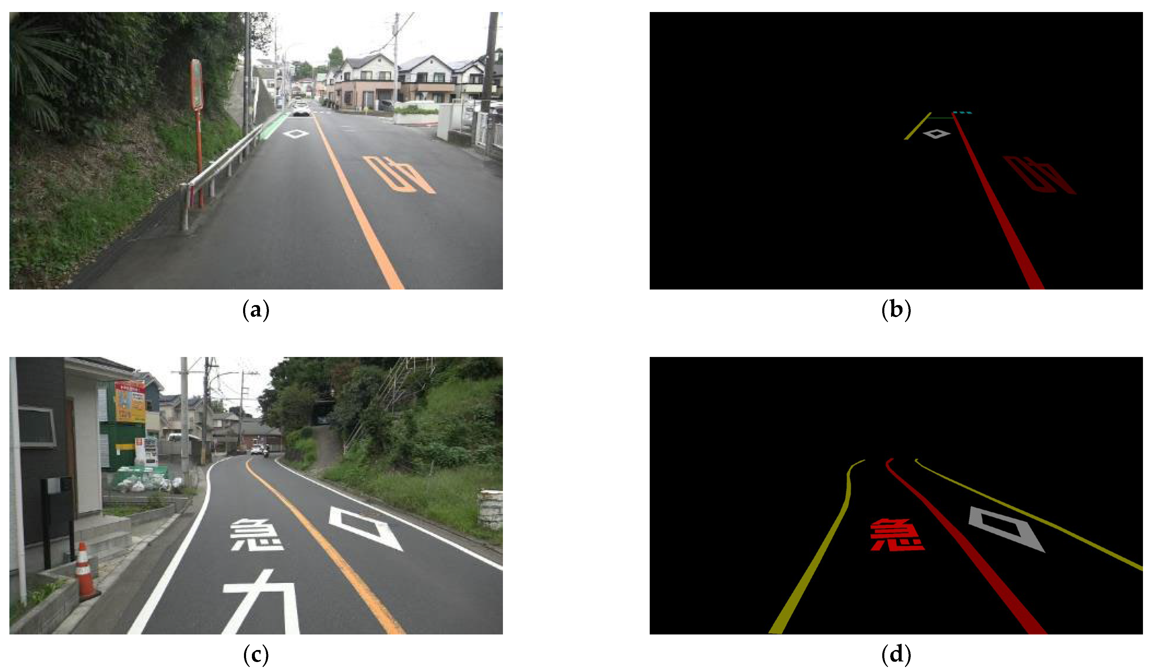
A graphical image-annotation tool called Labelme [39] was used to manually annotate the raw images. Both symbolic road markings and road lanes were manually annotated as polygons with corresponding shapes. After annotation, pixel-level segmentation masks were converted from the generated JSON format data. Examples of RMDs are shown in Figure 3. It should be noted that, when annotating road markings consisting of multiple Japanese characters, only the key characters were annotated, as shown in Figure 3d.

The RMD is divided into the training and test sets at a ratio of approximately 9:1, which correspond to 2990 and 321 images, respectively.

Table 2. Summary of the Road Marking Dataset (RMD) compiled by this study.

ID	RGB	Category	Training Set	Test Set	Total
0	0,0,0	Background	2900	321	3221
1	128,0,0	Yellow solid	676	66	742
2	0,128,0	Stop line	626	81	707
3	128,128,0	White solid	2119	222	2341
4	0,0,128	Left notice	56	7	63
5	128,0,128	Right notice	26	3	29
6	0,128,128	Pedestrian crossing	1024	109	1133
7	128,128,128	Approach to pedestrian and bicycle crossing	311	39	350
8	64,0,0	Maximum speed limit 40	139	19	158
9	192,0,0	Sharp-turn notice	34	5	39
10	64,0,128	School-zone notice	33	4	37
11	192,128,0	White broken	368	40	408
12	64,0,128	White dotted	183	24	207
13	192,0,128	Slow-down marking	75	16	91
14	64,128,128	Slow-down notice	33	6	39
15	192,128,128	Straight	87	11	98
16	0,192,0	Stop notice	52	5	57
17	128,192,0	+-shaped road intersection	6	2	8
18	0,64,128	T-shaped road intersection	55	11	66
19	128,64,128	Maximum speed limit 20	124	18	142
20	0,192,128	Right	17	2	19
21	128,192,128	Maximum speed limit 50	48	7	55
22	64,64,0	Straight-plus-left notice	11	4	15
23	192,64,0	Straight plus left	92	8	100
24	64,192,0	Left-curve notice	75	18	93
25	192,192,0	Notice	14	4	18
26	0,192,128	Left	18	9	27
27	192,64,128	Bicycle crossing	9	2	11
28	64,192,128	Straight notice	13	5	18
29	192,192,128	Maximum speed limit 30	32	5	37

shows the ID and RGB value of each category, and the numbers of images for each category in the training set, test set, and the total. Because the road surface in each image may involve several road markings (Figure 1e), including the same road marking in plural, the number of instances of each category is more than the number of images for each category. The RMD needs to be perfected by adding more road-surface images with symbolic road markings due to the problem of class imbalance, shown in Table 2.

4. Proposed Method

4.1. Overview of Proposed Method

In this study, we propose a novel multiscale attention-based dilated convolutional neural network (MSA-DCNN) to tackle the RMD. The structure of the MSA-DCNN is similar to the image pyramid shown in Figure 2a. The most intuitive examples of Figure 2a are the average pooling and max pooling over two input scales. They can be considered as special cases of an attention mechanism applied to the image pyramid. Average pooling assigns the same weight to features at each scale, while max pooling assigns the weights of 0 and 1. In this study, unlike merging the predictions by average pooling or max pooling, we adopted an attention module that can softly weight the feature maps from different input scales [30,31]. The weights obtained by the attention module can reflect the importance of features at all the spatial positions from different input scales. The representation power of the CNN can be increased by the pixel-wise multiplication of the attention weights and feature maps, such that the attention mechanism allows the CNN to focus on features from important input scales, and it suppress features from the other input scales. As a result, the attention module decides the weight of a feature at the same position for each scale, and it increases the representation power of the CNN. In addition, dilated convolution [29] is used to enlarge the receptive field of feature maps and utilize a large range of spatial-context information. Hence, the MSA-DCNN can be seen as a combination of types, as shown in Figure 2a,c. The proposed MSA-DCNN is a share-net [30], where multiscale inputs are fed to an attention-weight-shared DCNN. The network for each scale is composed of a feature-extraction part, semantic head, and attention module. To be more specific, we explain the procedures of the training process and inference processes by two examples. The basic notations and meanings are defined in

Table 3. Notations and meanings for the proposed method.

Notations	Meanings
$s$	The scale of input
$scales=\langle s_1,s_2\rangle$	The list of input scales in the training process composed of $s_1$ and $s_2$
$scales=\left\{s_1,s_2\right\}$	The list of input scales in the inference process composed of $s_1$ and $s_2$
$p_s$	The semantic prediction of scale $s$ obtained by semantic head
${\alpha }_s$	The attention weights of scale $s$ obtained by attention module
$O_s$	The output mask of scales
$O_f$	The final output mask
$U$	The upsampling operation by bilinear interpolation
D	The downsampling operation by bilinear interpolation
$\ast$	The pixel-wise multiplication
$+$	The pixel-wise addition

.

4.1.1. Training Process

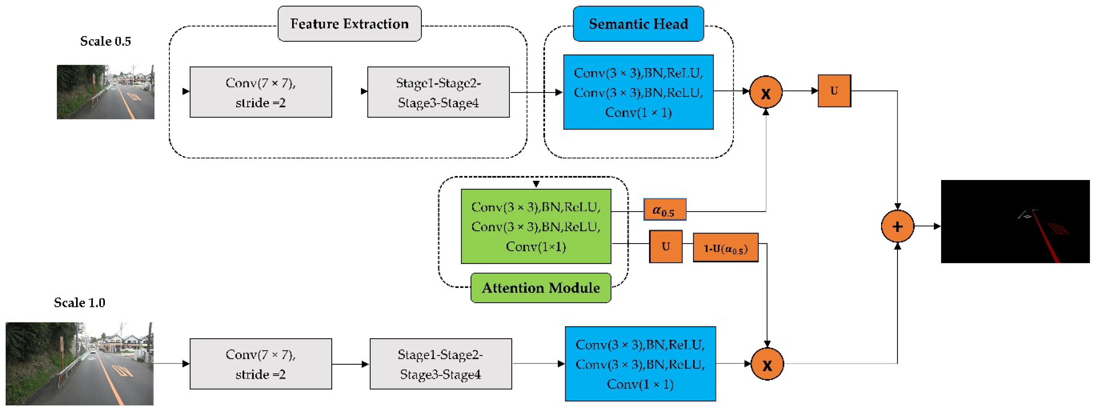
First, the original image is scaled by $s=0.5$ and $s=1.0$ ($s=0.5$ means that the number of pixels on a side is resized to $0.5$ times, while $s=1.0$ means no operation), such that we have multiscale inputs of $s=0.5$ and $s=1.0$, denoted as $scales=\langle 0.5,1.0\rangle$, as shown in Figure 4. Images at two scales are passed through the same feature-extraction part to obtain feature maps with semantic information. The feature maps then go through the semantic head and attention module. The semantic head performs the semantic prediction ($p_s$), and the attention module produces attention weights (${\alpha }_s$) over all spatial positions. It should be noted that the attention weights are learned from the adjacent scale pairs in the training process, which are the input scales of $s=0.5$ and $s=1.0$ in this example. The learned attention weights are considered relative attention weights between the adjacent scale pairs. Thereafter, the output mask $\left(O_{0.5}\right)$ of scale $s=0.5$ is produced by the pixel-wise multiplication of semantic prediction $p_{0.5}$ and attention weights ${\alpha }_{0.5}$. The equation can be formalized as:

$$O_{0.5}=p_{0.5}\ast {\alpha }_{0.5}$$

(1)

The output mask $\left(O_{1.0}\right)$ of scale $s=1.0$ is produced by the pixel-wise multiplication of semantic prediction $p_{1.0}$ and attention weights $\left(1-U({\alpha }_{0.5}\right))$, where $U$ represents the upsampling operation. The equation can be formalized as:

$$O_{1.0}=p_{1.0}\ast \left(1-U({\alpha }_{0.5}\right))$$

(2)

Thus, the final output ($O_f$), which is the same size as the original image, can be expressed with pixel-wise addition, denoted as $+$.

$$\begin{gathered} O_f=U(O_{0.5})+O_{1.0} \\ =U(p_{0.5}\ast {\alpha }_{0.5})+p_{1.0}\ast \left(1-U({\alpha }_{0.5}\right)) \end{gathered}$$

(3)

4.1.2. Inference Process

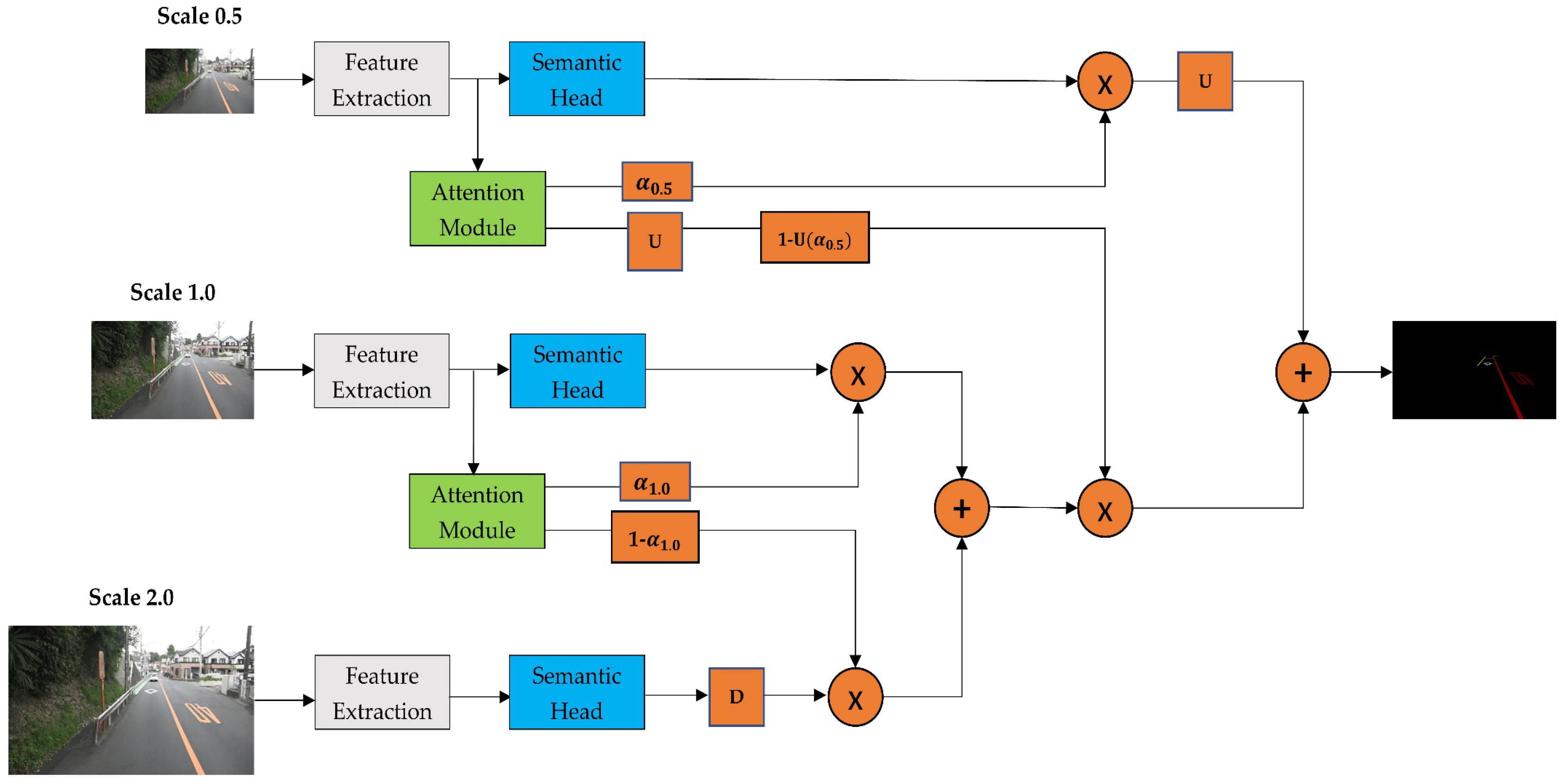
The procedure of the inference process is similar to that of the training process. Because the attention weights are learned between adjacent scales in the training process, different multiscale inputs can be selected at the inference time. Here, we explain the inference process using the three inputs, the scales of which are $s=0.5, s=1.0, \mathrm{and} s=2.0$, denoted as $scales=\left\{0.5,1.0,2.0\right\}$, as shown in Figure 5. We obtain the final output mask ($O_f$) by combining the semantic predictions of these three different scale inputs based on the attention modules.

First, the original image is scaled by $s=0.5$, $s=1.0$, and $s=2.0$ ($s=2.0$ means that the number of pixels on a side is resized to $2.0$ times), such that we have multiscale inputs of $s=0.5, s=1.0$, and $s=2.0$, denoted as $scales=\left\{0.5,1.0,2.0\right\}$. Images at three scales are passed through the feature-extraction part to obtain feature maps, and the semantic head to obtain semantic predictions. The output mask $\left(O_{1.0}\right)$ of scale $s=1.0$ is produced by the pixel-wise multiplication of semantic prediction $p_{1.0}$ and attention weights ${\alpha }_{1.0}$. The equation can be formalized as:

$$O_{1.0}=p_{1.0}\ast {\alpha }_{1.0}$$

(4)

The output mask $\left(O_{2.0}\right)$ of scale $s=2.0$ is produced by the pixel-wise multiplication of semantic prediction $D\left(p_{2.0}\right)$, where $D$ represents the downsampling operation, and attention weights $\left(1-{\alpha }_{1.0}\right)$. The equation can be formalized as:

$$O_{2.0}=D(p_{2.0})\ast (1-{\alpha }_{1.0})$$

(5)

The output mask $\left(O_{0.5}\right)$ of scale $s=0.5$ is produced by the pixel-wise multiplication of semantic prediction $p_{0.5}$ and attention weights ${\alpha }_{0.5}$. The equation can be formalized as:

$$O_{0.5}=p_{0.5}\ast {\alpha }_{0.5}.$$

(6)

Thus, for the final output ($O_f$), the equation can be formalized as:

$$O_f=U\left(p_{0.5}\ast {\alpha }_{0.5}\right)+\left(p_{1.0}\ast {\alpha }_{1.0}+D\left(p_{2.0}\right)\ast \left(1-{\alpha }_{1.0}\right)\right)\ast \left(1-U\left({\alpha }_{0.5}\right)\right)$$

(7)

As described above, the training and inference processes are explained by the two examples. Multiscale inputs of $s=0.5$ and $s=1.0$, denoted as $scales=\langle 0.5,1.0\rangle$, are used in the example of the training process. The attention weights (${\alpha }_{0.5}$) of scale $s=0.5$ and the attention weights $\left(1-U({\alpha }_{0.5}\right))$ of scale $s=1.0$ are learned from the adjacent scale pairs of $s=0.5$ and $s=1.0$, respectively. Because the attention weights learned are relative, we can flexibly select the scales of the inputs at the inference time. For the example of the inference process, the multiscale inputs $s=0.5$, $s=1.0$, and $s=2.0$, denoted as $scales=\left\{0.5,1.0,2.0\right\}$, are used. The attention weights learned from the training process will be used in the inference process, and the learned attention weights can be rescaled by bilinear interpolation to fit the semantic predictions of different scales of inputs.

4.2. Feature Extraction

The feature-extraction part in the proposed method is a modified ResNet-50 [34] based on dilated convolution [29]. ResNet is widely used to design CNNs as a backbone, and dilated convolution is used to enlarge the receptive field of feature maps and utilize a large range of spatial-context information. Stage 1 and Stage 2 in the feature-extraction part represent the layers of conv2_x and conv3_x in ResNet-50 [34], while Stage 3 and Stage 4 are the modified layers of conv4_x and conv5_x in ResNet-50 [34], based on dilated convolution. We removed the striding in the layers of conv_4x and conv5_x by adding dilated convolution layers. ResNet-50 has five downsampling operations by conv1, max pool, conv3_1, conv4_1, and conv5_1, with a stride of 2, which makes the whole downsampling factor 32. However, our modified ResNet-50 has a downsampling factor of 8 to enlarge the receptive field of the feature maps.

Table 4. Comparison of the output size of the feature map caused by the downsampling operation in the feature-extraction part of the proposed method and the original ResNet-50.

Suppose the Crop Size is 1024 × 1024
Feature-extraction part	Downsampling	Conv7 × 7	Stage1	Stage2	Stage3	Stage4
	Output size	512 × 512	256 × 256	128 × 128	128 × 128	128 × 128
ResNet-50	Downsampling	Conv1	Conv2_x	Conv3_x	Conv4_x	Conv5_x
	Output size	512 × 512	256 × 256	128 × 128	64 × 64	32 × 32

shows the comparison of the output size of the feature map caused by the downsampling operation in the feature-extraction part of the proposed method and the original ResNet-50. It can be seen that the feature map is enlarged to preserve more spatial information by our feature-extraction part. The dilated convolution is embedded into the last two stages because avoiding the memory consumption caused by the high-resolution feature map and the downsampling factor of 8 is enough to preserve most of the spatial information [40].

4.3. Semantic Head and Attention Module

As mentioned earlier, the semantic predictions are performed by the semantic head, and the attention module produces the attention weights. The structures of the semantic head and attention module are identical, both consisting of Conv (3 × 3) (256), BN, ReLU, Conv (3 × 3) (256), BN, ReLU, and Conv (1 × 1) (dimension), as shown in Figure 4. Both the semantic head and attention module are fed with the final feature map from Stage 4 in the feature-extraction part. The only difference between the semantic head and attention module is the dimension of the final convolution output (conv1 × 1). For the semantic head, the number of channels of the final convolution output is consistent with the number of categories in the dataset. However, the attention module outputs a single channel, where the value of each position represents the weight of the corresponding position.

To be more specific, we discuss how the attention module merges the feature maps from multiscale inputs. Assuming that the spatial position of semantic prediction is $i$, and $c\in \left\{1,\dots ,C\right\}$, where $C$ is the number of categories, the semantic prediction can be denoted as $p_{i,c}^s$, where $s\in \left\{1,\dots ,S\right\}$ is the scale of the input. The attention module merges the semantic predictions from multiscale inputs to obtain the weighted sum, which is the output mask in this study. We denote $o_{i,c}$ as the output mask at the spatial position $i$ for the category $c$, and ${\alpha }_i^s$ as the attention weight at position $i$ for scale $s$, and we have:

$$o_{i,c}={\displaystyle \sum }_{j=1}^S{p}_{i,c}^s.{\alpha }_i^s$$

(8)

The attention weight (${\alpha }_i^s$) is computed as follows:

$${\alpha }_i^s=k_{1,1}\otimes max\left(0,k_{3,3}\otimes \max \left(0,k_{3,3}\otimes f_{S4}\right)\right)$$

(9)

where $\otimes$ denotes the convolution operation, $k_{1,1}$ and $k_{3,3}$ represent kernels with the sizes of $1\times 1$ and $3\times 3$, respectively, and $f_{S4}\in R^{Ch\times H\times W}$ is the final feature map from Stage 4 in the feature-extraction part. The attention module was designed to compute a soft weight at each spatial position for each scale. Because the convolution operation can extract informative spatial features, we designed the structure of the attention module as mentioned earlier. Furthermore, backpropagation is used to calculate the gradient of the loss function. As a result, the attention module decides the weight of a feature at the same position for each scale, and it increases the representation power of the CNN.

5. Results

5.1. Experimental Details

The proposed MSA-DCNN was trained using the RMD on a Linux Ubuntu 20.04 LTS with one NVIDIA GeForce RTX 3090 GPU with 24 GB video memory and the PyTorch framework. The batch size was set as 2. The stochastic gradient descent (SGD) with an original learning rate of 0.005, a momentum of 0.9, and a weight decay of 0.0001 was selected to optimize the proposed MSA-DCNN. We trained the models for 200 epochs. Random horizontal flipping, Gaussian blurring, color augmentation, and cropping were employed to augment the RMD. The cross entropy [41,42] was used as the loss function, which can be defined as follows:

$$L\left(y_{o,c},p_{o,c}\right)=-\frac{1}{m}{\displaystyle \sum }_{j=1}^m{\displaystyle \sum }_{i=1}^n{y}_{o,c}log\left(p_{o,c}\right)$$

(10)

where $m$ is the batch dimension, $n$ is the number of classes, $y$ is the binary indicator (if class label $c$ is the correct classification for observation $o$, $y=1$), and $p$ is the predicted probability that observation $o$ is of class $c$. To evaluate the proposed models, we used intersection over union (IoU) [43] as the metric, which can be defined as follows:

$$IoU=\frac{\left|A\cap B\right|}{\left|A\cup B\right|}$$

(11)

where $A$ is the ground truth, and $B$ is the predicted result.

5.2. Results of the Proposed Method

As mentioned in Section 4, the original image will be scaled by specific factors to compose scale pairs in the training process to learn the attention weights between adjacent scale pairs. In the example of the training process described in Section 4, the input scales of $s=0.5$ and $s=1.0$, denoted as $scales=\langle 0.5,1.0\rangle$, are used to explain the training process. In the experimental stage of this study, we trained the two models: Model 1 and Model 2. Model 1 employed scales of $s=0.5$ and $s=1.0$, denoted as $scales=\langle 0.5,1.0\rangle$, and Model 2 employed scales of $s=1.0$ and $s=2.0$, denoted as $scales=\langle 1.0,2.0\rangle$.

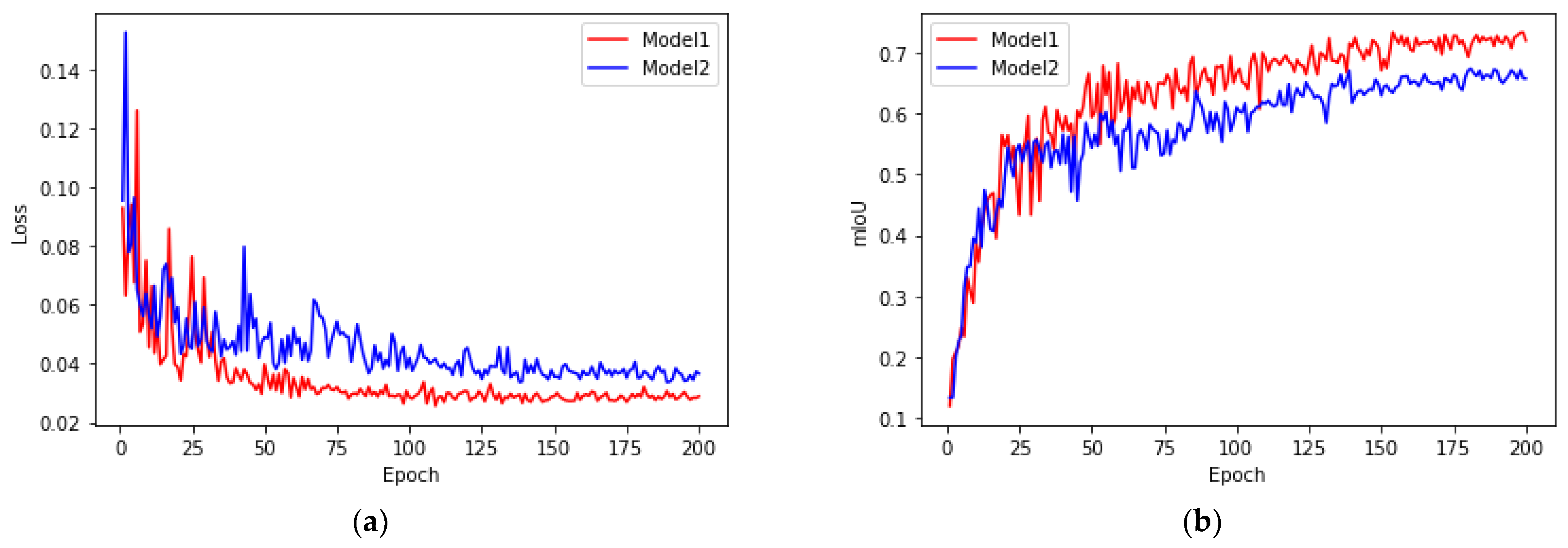
The loss and mean IoU (mIoU) values of the two models for the test set during the training process are shown in Figure 6. It should be noted that, when calculating the loss and mIoU, the images of the test set are scaled with the same factors as those of the training set. Model 1, with $scales=\langle 0.5,1.0\rangle$, gained the best mIoU (73.29%) for the epoch of 153, while Model 2, with $scales=\langle 1.0,2.0\rangle$, obtained the best mIoU (67.32%) for the epoch of 180. Model 1 and Model 2 learn the attention weights between specific adjacent scale pairs, which are $scales=\langle 0.5,1.0\rangle$ and $scales=\langle 1.0,2.0\rangle$, respectively.

In the example of the inference process described in Section 4, scales of $s=0.5, s=1.0,$ and $s=2.0$, denoted as $scales=\left\{0.5,1.0,2.0\right\}$, are used to explain the inference process. Because we can flexibly select multiple scales at the inference time, five kinds of multiscale inputs were selected to evaluate Model 1 and Model 2 in the experimental stage of this study: $scales=\left\{1.0,2.0\right\}$, $scales=\left\{0.5,1.0\right\}$, $scales=\left\{0.5,1.0,2.0\right\}$, $scales=\left\{0.25,0.5,1.0\right\}$, and $scales=\left\{0.25,0.5,1.0,2.0\right\}$. For example, $scales=\left\{0.25,0.5,1.0,2.0\right\}$ means that multiple scales of $s=0.25$, $s=0.5$, $s=1.0$, and $s=2.0$ are used as the inputs to evaluate the two models at the inference time.

Table 5. The mIoU values obtained by Model 1 and Model 2 with the five kinds of multiscale inputs.

Input Scale	mIoU
	Model 1	Model 2
$scales=\left\{1.0,2.0\right\}$	65.68	67.32
$scales=\left\{0.5,1.0\right\}$	73.29	74.41
$scales=\left\{0.5,1.0,2.0\right\}$	73.55	74.88
$scales=\left\{0.25,0.5,1.0\right\}$	72.45	73.73
$scales=\left\{0.25,0.5,1.0,2.0\right\}$	72.64	74.22

presents the mIoU values of Model 1 and Model 2 with five kinds of multiscale inputs in the inference process. It is shown that both Model 1 and Model 2 result in the best mIoU values: 73.55% for Model 1 and 74.88% for Model 2, when $scales=\left\{0.5,1.0,2.0\right\}$. Except for $scales=\left\{1.0,2.0\right\}$, the differences in the mIoU values obtained by Model 1 and Model 2 are not larger than 1.1% and 1.15%, respectively. Using the scale of $s=2.0$ will enhance the segmentation accuracy of smaller road markings, but it is not conducive to the segmentation of larger road markings. In contrast, using scales of $s=0.5$ and $s=0.25$ can improve the segmentation accuracy of larger road markings, but is not good at the segmentation of smaller road markings. We have observed that the number of road markings at a relatively large scale is significantly larger than that at a smaller scale in the RMD. This is considered the main reason for the low mIoU values on $scales=\left\{1.0,2.0\right\}$ compared with the others.

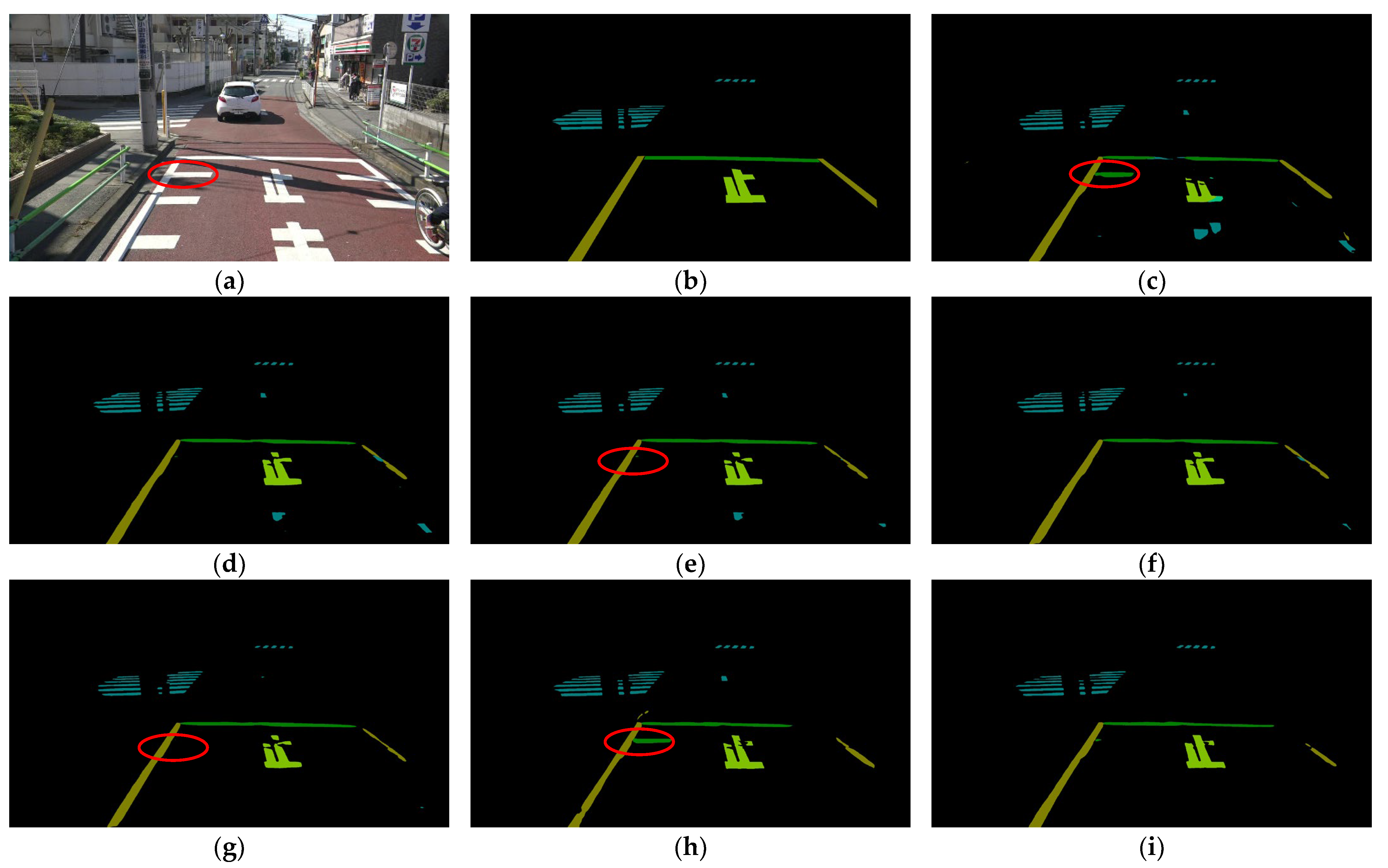
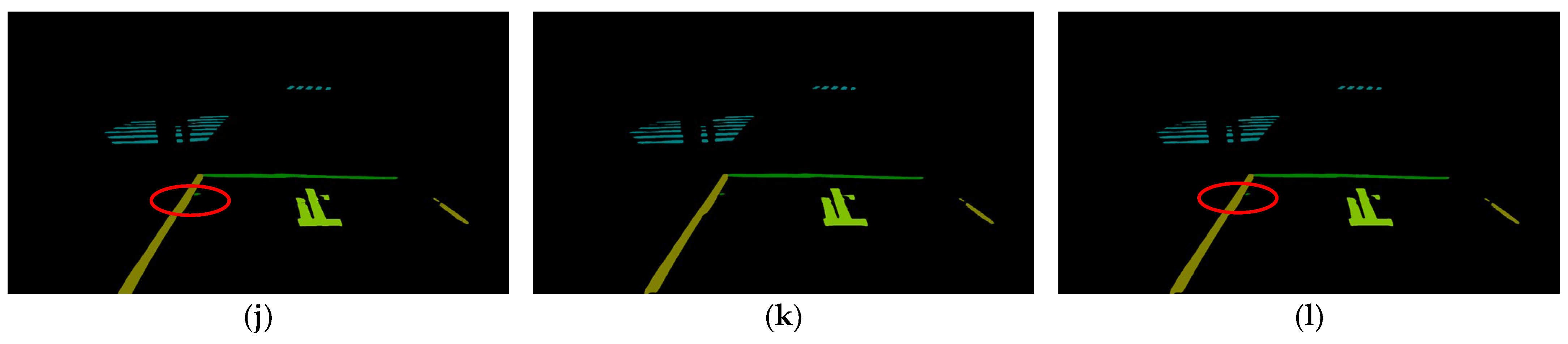
Examples of the results obtained by Model 1 and Model 2 with five kinds of multiscale inputs are shown in Figure 7. Apart from the result of $scales=\left\{1.0,2.0\right\}$, the results of the other multiscale inputs seem to be credible. For the result of $scales=\left\{1.0,2.0\right\}$ obtained by Model 1 (Figure 7c) and Model 2 (Figure 7h), a clear misprediction indicated by the red ellipse can be observed. We assume that the short white line in the red ellipse was incorrectly predicted as the stop line because the scale $s=2.0$ was used to allow the network to pay more attention to the fine details. However, the other multiscale inputs (Figure 7e,g,j,l) containing scale $s=2.0$ do not show this trend. We believe that scale $s=0.5$ successfully weakens the effect of scale $s=2.0$ because there are more relatively large road markings in the RMD.

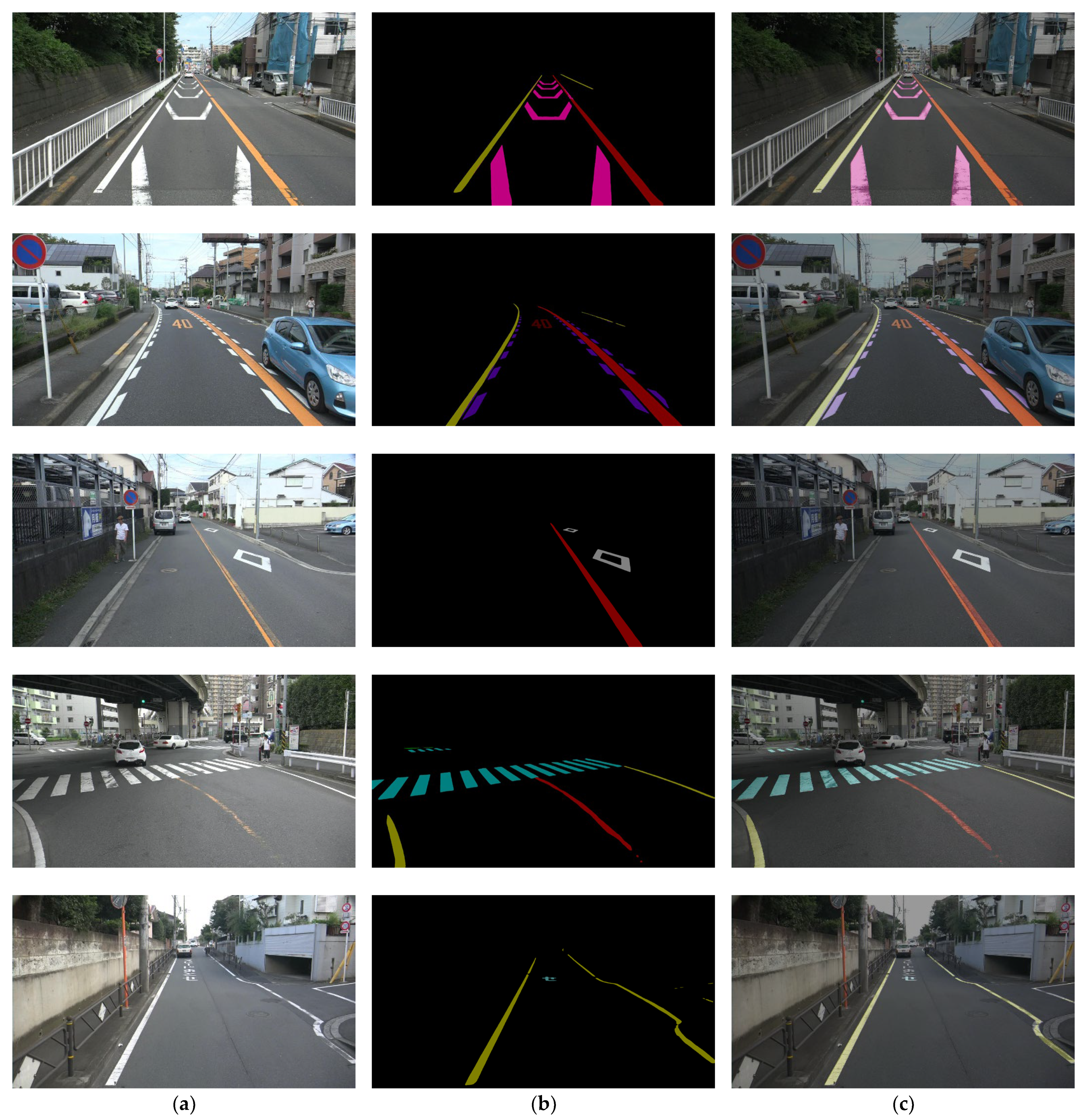
In addition, the best results obtained by Model 2 with $scales=\left\{0.5,1.0,2.0\right\}$ are shown in

Table 6. IoU of each category obtained by Model 2 with $scales=\left\{0.5,1.0,2.0\right\}$.

Category	IoU
Background	99.08
Yellow solid	83.62
Stop line	58.42
White solid	71.46
Left notice	60.23
Right notice	52.62
Pedestrian crossing	82.16
Approach to pedestrian and bicycle crossing	85.91
Maximum speed limit 40	77.98
Sharp-turn notice	78.04
School-zone notice	81.65
White broken	65.49
White dotted	82.71
Slow-down marking	85.19
Slow-down notice	82.82
Straight	75.42
Stop notice	83.93
+-shaped road intersection	79.85
T-shaped road intersection	85.40
Maximum speed limit 20	79.11
Right	82.64
Maximum speed limit 50	73.61
Straight-plus-left notice	83.41
Straight plus left	50.68
Left-curve notice	52.01
Notice	63.73
Left	82.37
Bicycle crossing	72.22
Straight notice	65.78
Maximum speed limit 30	68.95
mIoU	74.88
mIoU (29 road-marking categories)	74.05

(IoU of each class), and some examples are illustrated in Figure 8. Excluding the background, the model achieved a 74.05% mIoU. Overall, half of the road markings have IoU values greater than 75%. Regardless of the distance between the road markings and the camera inside the vehicle, the road markings at a large scale, such as the pedestrian crossing and slow-down marking, are better segmented, achieving IoU values of more than 80%. At the same time, those that achieved lower IoU values are generally road markings at a small scale. Hence, perfecting the proposed RMD by adding images of road-surface scenes with road markings at a smaller scale becomes more crucial. The illustration of some prediction results shows that the model reproduces the overall features of the road markings. The first row of Figure 8 shows that the model can detect deteriorated road markings. We can also see that the model can detect road markings in shadow, as shown in the fourth row of Figure 8.

5.3. Performance Analysis

To validate the performance of the proposed MSA-DCNN, a performance analysis was conducted. Because the multiscale attention module and dilated convolution are the core ideas adopted, we set up three additional experiments, as shown in

Table 7. Performance analysis on the test dataset of RMD.

No.	Multiscale Attention	Dilated Convolution	mIoU
1			67.24
2		√	69.35
3	√		71.07
4	√	√	74.88

. We evaluated the model with ResNet-50 [34]-based feature extraction as the baseline model (No. 1) on the test dataset of the RMD, and we obtained a 67.24% mIoU. The second model (No. 2), with our modified ResNet-50 as the feature-extraction part, outperformed the baseline model by a gain of 2.11% mIoU. The multiscale attention-based CNN [31] without dilated convolution in the feature-extraction part (No. 3) resulted in a gain of 1.72% mIoU compared with No. 2. Finally, the proposed MSA-DCNN acquired the top value of a 74.88% mIoU. The ablation study shows that the proposed MSA-DCNN yields the best results combining multiscale attention and dilated convolution.

5.4. Comparisons with Other Models

The proposed method was designed to tackle the problem of the existence of objects at multiple scales of the RMD, as mentioned in Section 4.1. Moreover, our proposed method is a combination of two types of methods to handle the problems that are the image pyramid (Figure 2a) and dilated convolution (Figure 2c). It is reasonable to compare the proposed method with other types of methods (i.e., encoder–decoder, dilated convolution, and pyramid pooling). Hence, we selected three representative state-of-the-art models, U-Net [36], PSPNet [38], and DeepLabV3+ [37], to compare with our proposed method.

The proposed method outperforms all the compared models in terms of the mIoU, as shown in

Table 8. Comparison of the results.

Model	mIoU
U-Net [36]	68.79
PSPNet [38]	71.42
DeepLabV3+ [37]	73.82
MSA-DCNN (this study)	74.88

. DeepLabV3+ achieves a better result than U-Net and PSPNet because it adopts dilated convolution and ASPP based on an encoder–decoder structure. The PSPNet yields a better result than U-Net, as the PPM of the PSPNet can provide additional context information in the semantic-segmentation task, while U-Net only adopts the encoder–decoder structure among the four types of methods shown in Figure 3. However, the training process of the proposed method is time consuming, taking approximately 78 h on an NVIDIA GeForce RTX 3090 GPU, while the three compared models take less than 48 h.

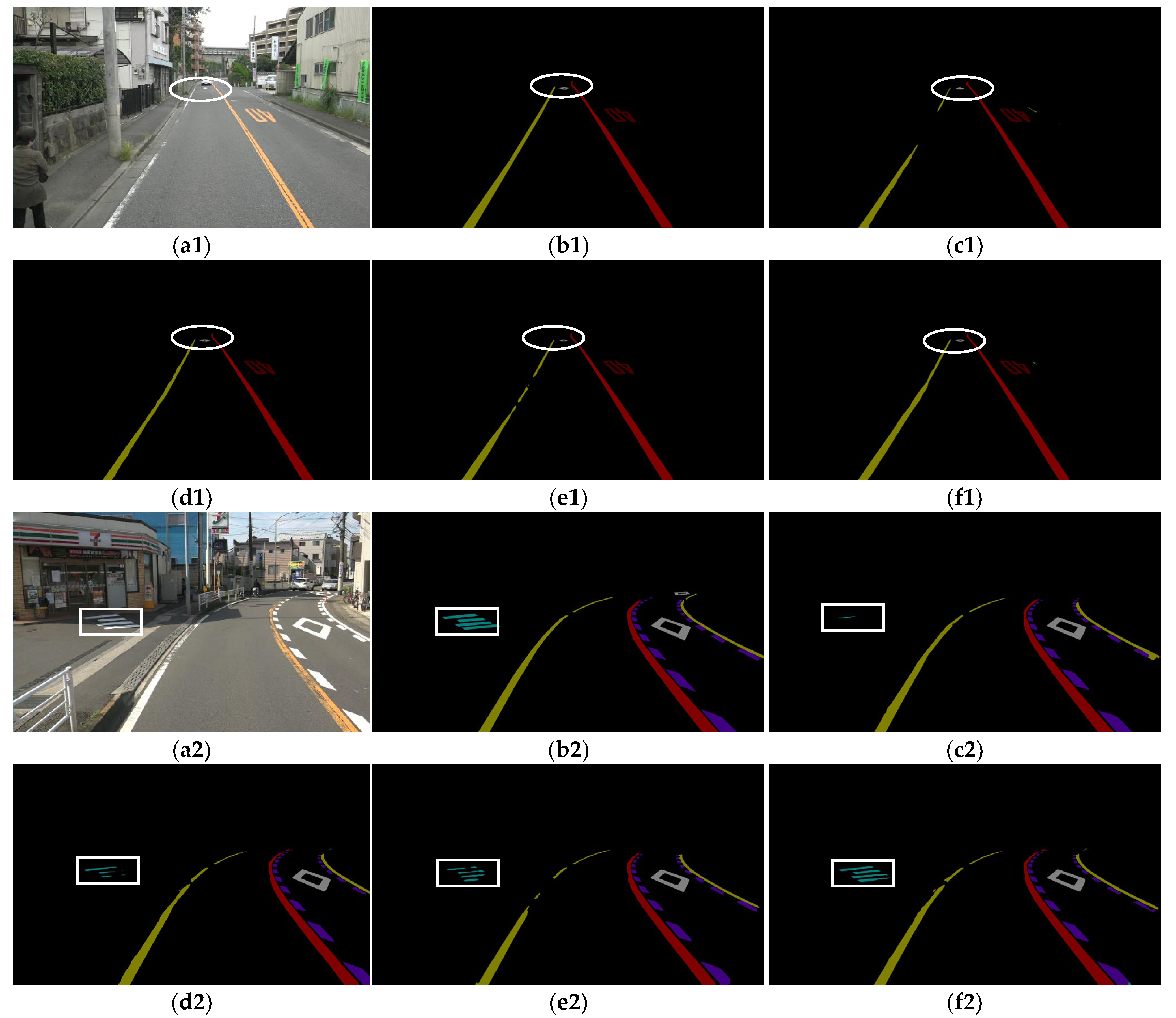
Figure 9 presents the visual results of the four models on the two test images of the RMD. In Figure 9(a1–f1) shows that U-Net and the PSPNet fail to finely segment the road marking of the approach to the pedestrian and bicycle crossing in the distance (as highlighted by the white ellipse). It can be observed that DeepLabV3+ and the proposed method improve the accuracy of the boundary segmentation. The proposed method obtains a better result compared with the others, as it uses multiscale inputs to improve the segmentation accuracy of the fine detail. In Figure 9(a2–f2) shows that the segmentation results of the pedestrian crossing (as highlighted by white rectangles) of U-Net completely fail, and those of the PSPNet and DeepLabV3+ are irregular due to shadows. The segmentation result of the proposed method is more similar to the ground truth.

6. Conclusions

In this study, a new dataset for the semantic segmentation of road markings named the RMD is introduced. The RMD is proposed to compensate for the lack of datasets and the limitations of the existing datasets in the field of road-marking recognition. The proposed RMD comprises 3221 pixel-level well-annotated road-surface images of 29 road-marking categories, with a resolution of 1920 × 1080. It is divided into the training and test sets at a ratio of approximately 9:1, which correspond to 2990 and 321 images, respectively.

We focus on the problem of the existence of objects at multiple scales of the proposed RMD, and we investigate four kinds of network architectures that deal with the multiscale context. Inspired by previous studies, we propose a novel MSA-DCNN to tackle the RMD. An attention module that can softly weight the feature maps from different scales and dilated convolution to enlarge the receptive field of feature maps and utilize a large range of spatial-context information are adopted. The two models that employ $scales=\langle 0.5,1.0\rangle$ (Model 1) and $scales=\langle 1.0,2.0\rangle$ (Model 2) are trained to evaluate five kinds of multiscale inputs on the RMD. At the inference time, Model 2, with $scales=\left\{0.5,1.0,2.0\right\}$, gained the best mIoU of 74.88%. The ablation study shows that the proposed MSA-DCNN yields the best results by combining multiscale attention and dilated convolution. Additionally, it obtains better results in comparison with other state-of-the-art models.

The RMD should be constantly improved by adding more road-surface images with symbolic road markings due to the problem of class imbalance. In this study, we proposed the MSA-DCNN, which focuses on the accuracy of the segmentation rather than real-time segmentation. For a future study, we will work on designing a real-time accurate road-marking-segmentation algorithm to solve the diverse needs in the field of road-marking recognition.

References

- Neven, D.; Brabandere, B.D.; Georgoulis, S.; Proesmans, M.; Gool, L.V. Towards End-to-End Lane Detection: An Instance Segmentation Approach. In Proceedings of the 2018 IEEE Intelligent Vehicles Symposium (IV), Changshu, China, 26–30 June 2018. [Google Scholar]
- Geiger, A.; Lauer, M.; Wojek, C.; Stiller, C.; Urtasun, R. 3D Traffic Scene Understanding from Movable Platforms. IEEE Trans. Pattern Anal. Mach. Intell. 2014, 36, 1012–1025. [Google Scholar] [CrossRef] [PubMed]
- Pan, X.; Shi, J.; Luo, P.; Wang, X.; Tang, X. Spatial as Deep: Spatial CNN for Traffic Scene Understanding. In Proceedings of the Thirty-Second AAAI Conference on Artificial Intelligence, New Orleans, LA, USA, 2–7 February 2018. [Google Scholar]
- Massimo, B.; Alberto, B. GOLD: A Parallel Real-Time Stereo Vision System for Generic Obstacle and Lane Detection. IEEE Trans. Image Process 1998, 7, 62–81. [Google Scholar]
- Pizzati, F.; Allodi, M.; Barrera, A.; García, F. Lane Detection and Classification Using Cascaded CNNs. In Proceedings of the Computer Aided Systems Theory—EUROCAST 2019: 17th International Conference, Las Palmas de Gran Canaria, Spain, 17–22 February 2019. [Google Scholar]
- Aly, M. Real time detection of lane markers in urban streets. In Proceedings of the 2008 IEEE Intelligent Vehicles Symposium (IV), Eindhoven, The Netherlands, 4–6 June 2008. [Google Scholar]
- Chang, D.; Chirakkal, V.; Goswami, S.; Hasan, M.; Jung, T.; Kang, J.; Kee, S.K.; Lee, D.; Singh, A.P. Multi- Lane Detection Using Instance Segmentation and Attentive Voting. In Proceedings of the 2019 International Conference on Control, Automation and Systems (ICCAS 2019), Jeju, Korea, 15–18 October 2019. [Google Scholar]
- Hou, Y.; Ma, Z.; Liu, C.; Loy, C.C. Learning Lightweight Lane Detection CNNs by Self Attention Distillation. In Proceedings of the 2019 IEEE/CVF International Conference on Computer Vision (ICCV 2019), Seoul, Korea, 27 October–2 November 2019. [Google Scholar]
- Wang, Z.; Ren, W.; Qiu, Q. LaneNet: Real-time lane detection networks for autonomous driving. arXiv 2018, arXiv:1807.01726. Available online: https://arxiv.org/abs/1807.01726 (accessed on 22 June 2022).
- Ko, Y.; Lee, Y.; Azam, S.; Munir, F.; Jeon, M.; Pedrycz, W. Key Points Estimation and Point Instance Segmentation Approach for Lane Detection. IEEE Trans. Intell. Transp. Syst. 2021, 23, 8949–8958. [Google Scholar] [CrossRef]
- Qin, Z.; Wang, H.; Liu, X. Ultra Fast Structure-Aware Deep Lane Detection. In Proceedings of the 2020 European Conference on Computer Vision (ECCV 2020), Online, 23–28 August 2020. [Google Scholar]
- Chen, P.R.; Lo, S.Y.; Hang, H.M.; Chan, S.W.; Jhih, L.J. Efficient Road Lane Marking Detection with Deep Learning. In Proceedings of the 2018 IEEE International Conference on Digital Signal Processing (DSP), Shanghai, China, 19–21 November 2018. [Google Scholar]
- What is Road Marking? Available online: https://roadgrip.co.uk/blog/what-is-road-marking (accessed on 12 June 2022).
- Liu, X.; Deng, Z.; Lu, H.; Cao, L. Benchmark for road marking detection: Dataset specification and performance baseline. In Proceedings of the 2017 IEEE International Conference on Intelligent Transportation Systems (ITSC 2017), Yokohama, Japan, 16–19 October 2017. [Google Scholar]
- Fritsch, J.; Kuehnl, T.; Geiger, A. A New Performance Measure and Evaluation Benchmark for Road Detection Algorithms. In Proceedings of the 16th International Conference on Intelligent Transportation Systems (ITSC 2013), The Hague, The Netherlands, 6–9 October 2013. [Google Scholar]
- Cordts, M.; Omran, M.; Ramos, S.; Rehfeld, T.; Enzweiler, M.; Benenson, R.; Franke, U.; Roth, S.; Schiele, B. The Cityscapes Dataset for Semantic Urban Scene Understanding. In Proceedings of the 2016 IEEE Conference on Computer Vision and Pattern Recognition (CVPR 2016), Las Vegas, NE, USA, 27–30 June 2016. [Google Scholar]
- Neuhold, G.; Ollmann, T.; Bulò, S.R.; Kontschieder, P. The Mapillary Vistas Dataset for Semantic Understanding of Street Scenes. In Proceedings of the 2017 International Conference on Computer Vision (ICCV 2017), Venice, Italy, 22–29 October 2017. [Google Scholar]
- Brostow, G.J.; Shotton, J.; Fauqueur, J.; Cipolla, R. Segmentation and Recognition Using Structure from Motion Point Clouds. In Proceedings of the 2008 European Conference on Computer Vision (ECCV 2008), Munich, Germany, 8–14 September 2018; pp. 44–57. [Google Scholar]
- Yu, F.; Chen, H.; Wang, X.; Xian, W.; Chen, Y.; Liu, F.; Madhavan, V.; Darrell, T. BDD100K: A Diverse Driving Dataset for Heterogeneous Multitask Learning. arXiv 2018, arXiv:1805.04687v2. Available online: htttp://arxiv.org/abs/1805.04687 (accessed on 14 June 2022).
- Tusimple Competitions for CVPR2017. Available online: http://github.com/TuSimple/tusimple-benchmark (accessed on 23 June 2022).
- Xu, H.; Wang, S.; Cai, X.; Zhang, W.; Liang, X.; Li, Z. CurveLane-NAS: Unifying Lane-Sensitive Architecture Search and Adaptive Point Blending. In Proceedings of the 2020 European Conference on Computer Vision (ECCV 2020), Online, 23–28 August 2020. [Google Scholar]
- Wu, T.; Ranganathan, A. A practical system for road marking detection and recognition. In Proceedings of the 2012 IEEE Intelligent Vehicles Symposium (IV), Madrid, Spain, 3–7 June 2012. [Google Scholar]
- Chen, T.; Chen, Z.; Shi, Q.; Huang, X. Road marking detection and classification using machine learning algorithms. In Proceedings of the 2015 IEEE Intelligent Vehicles Symposium (IV), Seoul, Korea, 28 July–1 June 2015. [Google Scholar]
- Zhang, D.; Fang, B.; Yang, W.; Luo, X.; Tang, Y. Robust inverse perspective mapping based on vanishing point. In Proceedings of the 2014 IEEE International Conference on Security, Pattern Analysis, and Cybernetics (SPAC), Wuhan, China, 18–19 October 2014. [Google Scholar]
- Lee, S.; Kim, J.; Yoon, J.S.; Shin, S.; Bailo, O.; Kim, N.; Lee, T.H.; Hong, S.K.; Han, S.H.; Kweon, I.S. VPGNet: Vanishing Point Guided Network for Lane and Road Marking Detection and Recognition. In Proceedings of the 2017 International Conference on Computer Vision (ICCV 2017), Venice, Italy, 22–29 October 2017. [Google Scholar]
- Jang, W.; Hyun, J.; An, J.; Cho, M.; Kim, E. A Lane-Level Road Marking Map Using a Monocular Camera. IEEE CAA J. Autom. Sin. 2022, 9, 187–204. [Google Scholar] [CrossRef]
- Yu, Z.; Ren, X.; Huang, Y.; Tian, W.; Zhao, J. Detecting Lane and Road Markings at A Distance with Perspective Transformer Layers. In Proceedings of the 23rd IEEE International Conference on Intelligent Transportation Systems (ITSC), Rhodes, Greece, 20–23 September 2020. [Google Scholar]
- Jayasinghe, O.; Hemachandra, S.; Anhettigama, D.; Kariyawasam, S.; Rodrigo, R.; Jayasekara, P. CeyMo: See More on Roads—A Novel Benchmark Dataset for Road Marking Detection. In Proceedings of the 2022 IEEE/CVF Winter Conference on Applications of Computer Vision (WACV 2022), Waikoloa, HI, USA, 4–8 January 2022. [Google Scholar]
- Chen, L.C.; Papandreou, G.; Schroff, F.; Adam, H. Rethinking atrous convolution for semantic image segmentation. arXiv 2017, arXiv:1706.05587v2. Available online: https://arxiv.org/abs/1706.05587?context=cs (accessed on 24 June 2022).
- Chen, L.C.; Yang, Y.; Wang, J.; Xu, W.; Yuille, A.L. Attention to Scale: Acale-aware Semantic Image Segmentation. In Proceedings of the 2016 IEEE Conference on Computer Vision and Pattern Recognition (CVPR 2016), Las Vegas, NE, USA, 27–30 June 2016. [Google Scholar]
- Tao, A.; Sapra, K.; Catanzaro, B. Hierarchical multi-scale attention for semantic segmentation. arXiv 2020, arXiv:2005.10821. Available online: https://arxiv.org/abs/2005.10821 (accessed on 22 June 2022).
- Chang, C.Y.; Lin, C.H. An Efficient Method for Lane-Mark Extraction in Complex Conditions. In Proceedings of the 9th International Conference on Ubiquitous Intelligence and Computing and 9th International Conference on Autonomic and Trusted Computing, Fukuoka, Japan, 4–7 September 2012. [Google Scholar]
- Lu, P.; Cui, C.; Xu, S.; Peng, H.; Wang, F. SUPER: A Novel Lane Detection System. IEEE Trans. Intell. Veh. 2021, 6, 583–593. [Google Scholar] [CrossRef]
- He, K.; Zhang, X.; Ren, S.; Sun, J. Deep residual learning for image recognition. In Proceedings of the 2016 IEEE Conference on Computer Vision and Pattern Recognition (CVPR 2016), Las Vegas, NE, USA, 27–30 June 2016. [Google Scholar]
- Long, J.; Shelhamer, E.; Darrell, T. Fully Convolutional Networks for Semantic Segmentation. In Proceedings of the 2015 IEEE Conference on Computer Vision and Pattern Recognition (CVPR 2015), Boston, MA, USA, 7–12 June 2015. [Google Scholar]
- Ronneberger, O.; Fischer, P.; Brox, T. U-net: Convolutional networks for biomedical image segmentation. In Proceedings of the 18th International Conference on Medical Image Computing and Computer Assisted Intervention (MICCAI 15), Munich, Germany, 5–9 October 2015. [Google Scholar]
- Chen, L.C.; Zhu, Y.; Papandreou, G.; Schroff, F.; Adam, H. Encoder-decoder with Atrous Separable Convolution for Semantic image Segmentation. In Proceedings of the 2018 European Conference on Computer Vision (ECCV 2018), Munich, Germany, 8–14 September 2018. [Google Scholar]
- Zhao, H.; Shi, J.; Qi, X.; Wang, X.; Jia, J. Pyramid Scene Parsing Network. In Proceedings of the 2017 IEEE Conference on Computer Vision and Pattern Recognition (CVPR 2017), Honolulu, HI, USA, 21–26 July 2017. [Google Scholar]
- Wada, K. Labelme: Image Polygonal Annotation with Python. Available online: http://github.com/wkentaro/labelme (accessed on 23 June 2022).
- Yu, F.; Koltun, V.; Funkhouser, T. Dilated Residual networks. In Proceedings of the 2017 IEEE Conference on Computer Vision and Pattern Recognition (CVPR 2017), Honolulu, HI, USA, 21–26 July 2017. [Google Scholar]
- CROSSENTROPYLOSS. Available online: http://pytorch.org/docs/stable/generated/torch.nn.CrossEntropyLoss.html (accessed on 25 June 2022).
- Loss Functions, Cross-Entropy. Available online: http://ml-cheatthedocs.io/en/latest/loss_functions.html (accessed on 25 June 2022).
- Rahman, M.A.; Wang, Y. Optimizing Intersection-Over-Union in Deep Neural Networks for Image Segmentation. In Proceedings of the 12th International Symposium on Visual Computing (ISVC 2016), Las Vegas, NE, USA, 12–14 December 2016. [Google Scholar]
Figure 1.
Some examples of road markings on road surfaces: (a) white solid, maximum speed limit 40, yellow solid, and left-curve notice (ordinary); (b) stop notice and stop line (shadow); (c) pedestrian crossing and stop line (dazzle light); (d) white solid, yellow solid, turn-right notice, and straight notice (occlusion); (e) white solid, maximum speed limit 40, school-zone notice, slow-down marking, and yellow solid (deteriorated road markings); (f) white solid, slow-down notice, stop notice, stop line, and +-shaped road intersection (narrow road).
Figure 2.
Four types of network architectures for multiscale contexts.
Figure 3.
Examples of RMD: (a,c) image of scene; (b,d) segmentation mask.
Figure 4.
The procedure of the training process of the proposed method.
Figure 5.
The procedure of the inference process of the proposed method.
Figure 6.
The loss and mIoU of Model 1 and Model 2 on the test set during the training process: (a) loss; (b) mIoU.
Figure 7.
Examples of results obtained by Model 1 and Model 2 with five kinds of multiscale inputs: (a) original input image; (b) ground truth; (c) prediction result of Model 1 with ; (d) prediction result of Model 1 with ; (e) prediction result of Model 1 with ; (f) prediction result of Model 1 with ; (g) prediction result of Model 1 with ; (h) prediction result of Model 2 with ; (i) prediction result of Model 2 with ; (j) prediction result of Model 2 with ; (k) prediction result of Model 2 with ; (l) prediction result of Model 2 with . The performances of multiscale inputs with on the short white line are highlighted by the red ellipses.
Figure 8.
Some examples of results obtained by Model 2 with : (a) original input image; (b) prediction result; (c) composited image.
Figure 9.
Visual results on two test images of the RMD: (a1,a2) original test image; (b1,b2) ground truth; (c1,c2) segmentation result of U-Net; (d1,d2) segmentation result of PSPNet; (e1,e2) segmentation result of DeepLabV3+; (f1,f2) segmentation result of MSA-DCNN. The white frameworks highlight the performance differences of four models.