Article

Characterization of the Land Deformation Induced by Groundwater Withdrawal and Aquifer Parameters Using InSAR Observations in the Xingtai Plain, China

1
College of Geological Engineering and Geomatics, Chang’an University, Xi’an 710054, China
2
Key Laboratory of Western China’s Mineral Resource and Geological Engineering, Ministry of Education, Xi’an 710054, China
*
Author to whom correspondence should be addressed.
Remote Sens. 2022, 14(18), 4488; https://doi.org/10.3390/rs14184488
Submission received: 15 August 2022 / Revised: 5 September 2022 / Accepted: 6 September 2022 / Published: 8 September 2022

Abstract

:
Long-term overexploitation of groundwater has led to significant land subsidence and ground fissures in the Xingtai plain. These geo-hazards have threatened the safety of buildings and infrastructures. It is extremely important to investigate the coupling relationship between land deformation and hydraulic head change for controlling land subsidence and mitigating ground fissures. In this study, we obtained the spatial and temporal evolution of land deformation in the Xingtai plain by using Envisat/ASAR data during 2009~2010 and Sentinel-1A data during 2015~2021. Combining InSAR results, head observations and geological data, we investigated the response of land deformation to head change and estimate the aquifer parameters. First, joint analysis of displacement time series and head changes infers that land subsidence was mainly caused by the inelastic compaction in aquitards. Compared with the subsidence patterns during 2009~2010, both the rate and spatial extent of land subsidence increased obviously during 2015~2021. Second, seasonal fluctuations in hydraulic head resulted in significant seasonal deformation with an amplitude of 10~30 mm and peak time of January~March, of which the spatial–temporal distribution was consistent with that of the rapid subsidence. Third, obvious differences in the deformation rate and seasonal amplitude were observed across the Longyao ground fissures and other three potential fissures during 2015~2021, suggesting that the activity of ground fissures increased compared with that during 2009~2010. Finally, using InSAR results and head observations, we estimated the elastic and inelastic skeletal storativity, with values ranging from 0.9 × 10⁻³ to 12.4 × 10⁻³ and 6.2 × 10⁻³ to 88.0 × 10⁻³, respectively. The comparison between elastic and inelastic skeletal storativity suggests that ~84.5% of total subsidence was irreversible and permanent.

1. Introduction

Pumping groundwater from confined aquifer systems leads to hydraulic head drops. As a result, the effective stress increases, there is compaction in the confined aquifer systems and the consequent subsidence occurs [1]. The water consumption in the North China Plain (NCP) is heavily dependent on groundwater [2,3]. The NCP has experienced long-term overexploitation of groundwater to meet the water demand since the 1960s, resulting in more than 20 groundwater depression cones [2], which lead to severe land subsidence [4]. Until 2010, more than two-thirds of the NCP suffered from land subsidence, of which the area with accumulated subsidence of more than 1 m reached 9620 km2, accounting for about 7% of the total area [5]. The land subsidence has brought damages to buildings and infrastructures and caused ground fissures in many cities of the NCP [6]. The large-scale serious subsidence induced by groundwater overexploitation has attracted attention from governments. Therefore, some policies for restricting groundwater exploitation and diversions of surface water were implemented in the early 2000s over the cities with the greatest water shortage and most serious subsidence [7,8], such as Beijing, Tianjin and Cangzhou, which have led to head rise and mitigated land subsidence [4]. However, the head declines show an accelerating trend in the Southern NCP [9], resulting in the subsidence center shifting to this region. Additionally, the spatial and temporal distributions of subsidence induced by groundwater withdrawal and the response of the confined aquifer system to head change are poorly understood and barely studied [10]. Therefore, in this study, we chose Xingtai, which has the most rapid subsidence and the most active fissures in the Southern NCP, as the study area to characterize the spatial and temporal evolution of land subsidence and investigate their relationships with hydraulic head changes, which are important for subsidence mitigation and groundwater management.
Observing the land deformation and investigating its coupling relationship with head changes remain challenging with the in situ point measurements such as leveling and Global Navigation Satellite System (GNSS), due to the long interval in time and the low density in space [11]. Synthetic Aperture Radar (SAR) and Interferometric SAR (InSAR), which have been widely used to map urban area characterization [12], monitor flood inundation [13,14,15], assess safety of infrastructure [16,17] and detect geologic hazard [18,19], offer an alternative way to characterize the land deformation induced by groundwater withdrawal with high spatial and temporal resolutions over large areas [20,21,22,23]. Additionally, the InSAR results have also been used to estimate the aquifer parameters and groundwater storage (GWS) depletion in the NCP [4,24] and other major aquifers around the world [25,26,27,28]. Previous studies have applied the InSAR method to monitor land deformation associated with hydraulic head change. Yang et al. [6] detected the land subsidence induced by groundwater exploitation and mapped activity of Longyao ground fissures in Xingtai, using ALOSPALSAR images from 2007~2010. Liu et al. [29] indicated that the Longyao ground fissure is controlled by the Longyao Fault and groundwater overexploitation. Li et al. [30] investigated the distribution of land subsidence with Sentnel-1A during 2017~2019. However, no studies on the response of confined aquifer system to head change and the estimation of skeletal storativity using InSAR measurements have been published.
In this study, we characterized the spatiotemporal variations of land deformation and ground fissures and quantified the aquifer parameters in the Xingtai plain with multiple SAR datasets, as well as head measurements. First, we used the Envisat/ASAR and Sentinel-1A datasets to detect the distribution of land deformation in Xingtai during 2009~2010 and 2015~2021. The responses of long-term deformation time series and seasonal deformation to the head change were analyzed. Then the spatial and temporal variabilities of deformation rate and seasonal amplitude were evaluated across the Longyao ground fissure and another three potential fissures. Finally, the elastic and inelastic skeletal storativity at observation well locations were estimated by using the seasonal and long-term components of deformation and head changes. This paper is organized as follows: Section 2 introduces the background of the study area and the used datasets. The methods of InSAR time series analysis, seasonal signals extraction and skeletal storativity estimation are presented in Section 3. Section 4 includes the results of spatial–temporal evolution of land deformation, the activity of ground fissures and the distributions of skeletal storativity. Section 5 discusses the uncertainty due to multi-sensor InSAR and the advantage of InSAR to characterize groundwater change. The conclusions are summarized in Section 6.

2. Study Area and Datasets
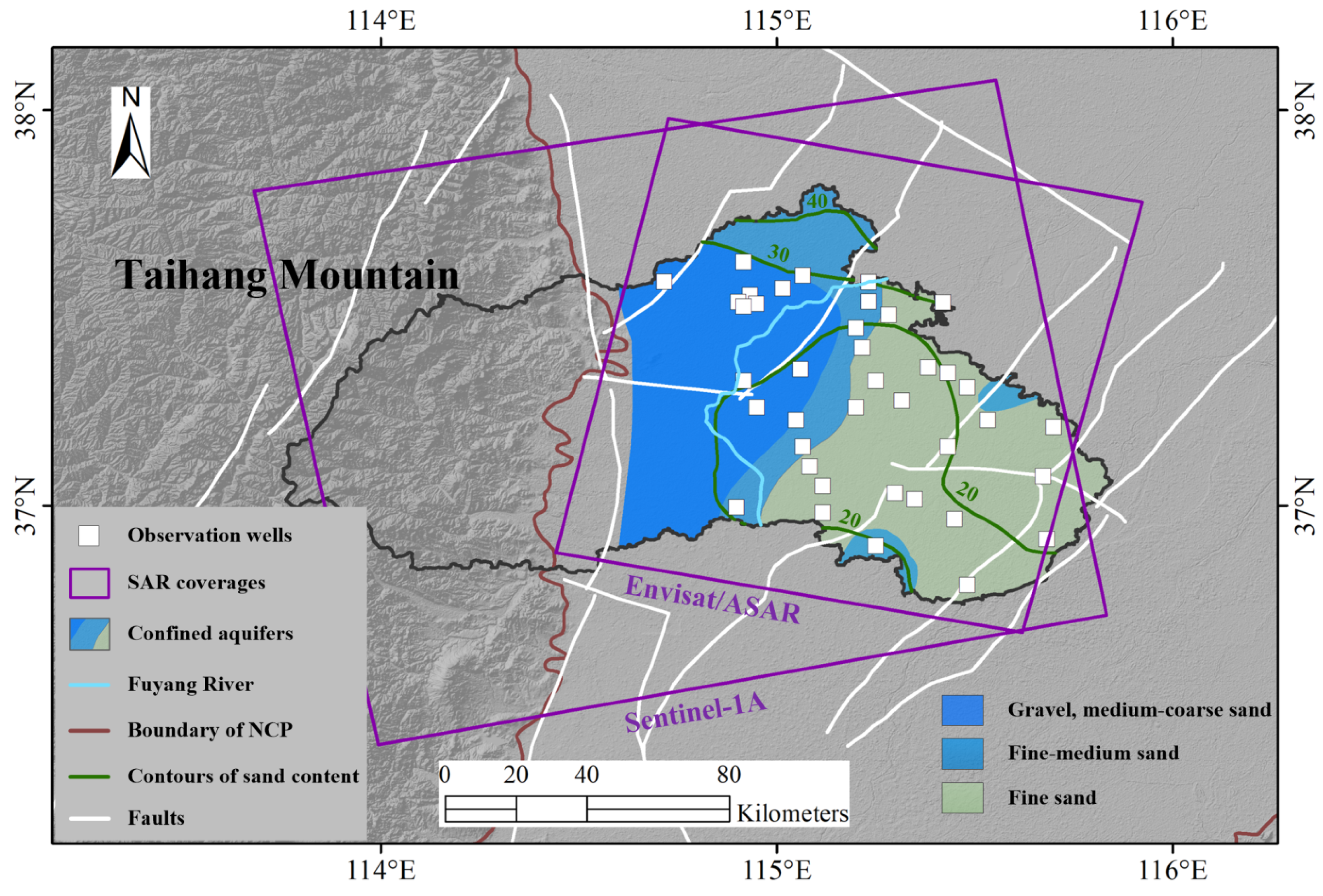
2.1. Study Area

Xingtai is located in the Southwestern NCP, which consists of mountainous and hilly areas in the west and a plain area in the east. Xingtai is characterized by an average annual temperature of 12~14 °C, as well as an average annual precipitation of 525 mm, 80% of which is concentrated from June to August [31]. The plain area, with an altitude varying from 30 to 100 m, is bounded by the Taihang Mountain to the west, accounting for ~70% of the total area. The Xingtai plain can be divided into piedmont alluvial–proluvial plain in the west of Fuyang River and eastern alluvial plain formed by the Yellow River and Ziya River in the east of the Fuyang River [32].
The aquifer system comprises an unconfined aquifer system in the upper layers and a confined aquifer system in the lower layers. The depths of the bottom of unconfined aquifer system and confined aquifer system are 20–140 m and 460–560 m in the piedmont alluvial–proluvial plain and 140–250 m and 520–580 m in the eastern alluvial plain, respectively [31]. The groundwater is mainly fresh, expect in the eastern alluvial plain, where the saline and fresh unconfined groundwater distribute alternately. The sediments in aquifers are composed of gravel and sand, becoming finer from west to east [31].
The agricultural, domestic and industrial water demands mainly rely on groundwater in the Xingtai plain. The long-term overexploitation of groundwater since the 1970s has resulted in a rapid head decline, forming the Ning-Bai-Long groundwater depression cone, with an area of 979 km2 and a maximum head drop of ~80 m until 2015 [33]. The rapid head decline has led to severe subsidence and ground fissures. More than 2 m of cumulative subsidence was measured up until 2015 [33], and tens of ground fissures have been found, including the Longyao ground fissure, which is the longest and most active fissure in the NCP [6,34]. To maintain the sustainability of the aquifer system, the government has restricted groundwater pumping since 2015 [31]. Additionally, the diverted water from the South-to-North Water Diversion Project (SNWDP) has replaced groundwater as the water source for domestic water use since June 2020 [35].

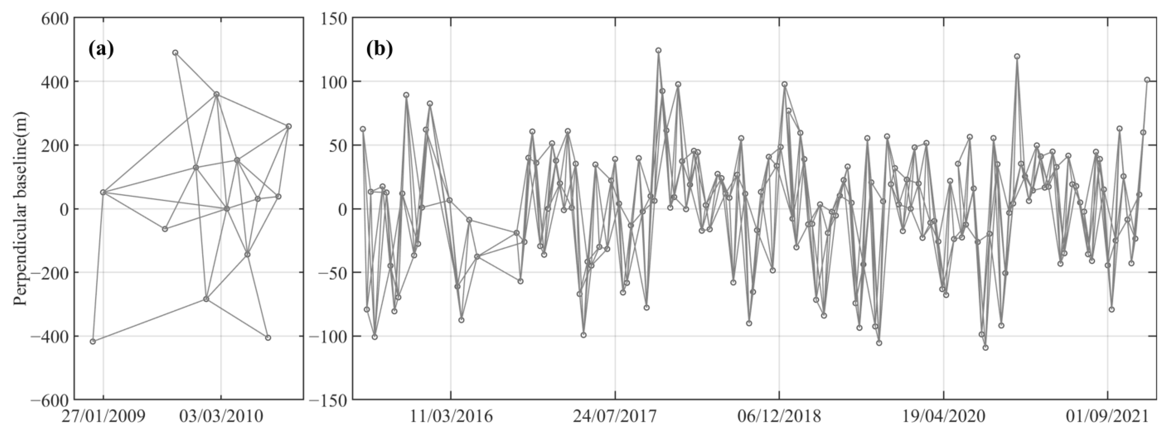
2.2. Datasets Used in the Study

In this study, 14 Envisat/ASAR images acquired during 2009~2010 and 178 Sentinel-1A images during 2015~2021 were collected to derive the deformation across Xingtai (the coverage shown in Figure 1). More detailed parameters of the SAR datasets are summarized in Table 1. The monthly hydraulic head measurements in the confined aquifer system at 39 wells (white boxes in Figure 1) during 2000~2017 were collected to investigate the relationship between groundwater change and land deformation and estimate the aquifer parameters.

3. Methods

3.1. Time-Series InSAR Analysis

To characterize the spatial–temporal evolution of land deformation in Xingtai, the StaMPS (Stanford Method for Persistent Scatter) method [36,37,38] was implemented with Envisat/ASAR images during 2009–2010 and Sentinel-1A images during 2015–2021. The thresholds of perpendicular and temporal baselines were respectively set as 500 m and 500 days for the Envisat/ASAR datasets and 120 m and 36 days for Sentinel-1A datasets for interferograms generation. Based on the joint analysis of the interferogram quality and coherence, a total of 33 interferograms from Envisat/ASAR and 516 interferograms from Sentinel-1A were finally selected (Figure 2). Then the topographic phase contribution in each interferogram was estimated and removed by using the 30 m resolution SRTM (Shuttle Radar Topography Mission) DEM.
We combined the amplitude and phase stability analysis to identify the PS (Persistent Scatterer) pixels [36]. The GACOS (generic atmospheric correction online service for InSAR) product [39,40,41] was used to remove the atmospheric phase disturbances. Then a 3D phase-unwrapping algorithm was used to recover the unambiguous phase values [42]. The orbital error was corrected by separating a linear phase ramp for each interferogram. Finally, the mean deformation rate and displacement time series along the line-of sight (LOS) direction were derived by using a least-squares inversion. Previous studies suggested that the horizontal deformation is negligible [6]; therefore, the LOS InSAR results were converted to vertical deformation based on the incident angle.

3.2. Extraction of Seasonal Deformation and Head Change

To evaluate the annual seasonal response of deformation to head change and estimate the elastic skeletal storativity, we used the harmonic function to isolate the seasonal displacement and head change [10]:
Y ( t ) = v t + A cos ( 2 π ( t T ) ) + B
where Y ( t ) is the time series of InSAR displacement or head observations, v is the linear trend of deformation and head, A is the amplitude of seasonal signal, t is time, T is the peak time corresponding to the peak surface uplift or head rise, and B is a constant. The amplitude (A) and peak time (T) can be estimated by using a least-squares inversion.

3.3. Estimation of Skeletal Storativity

Storativity indicates the amount of water taken into or released from unit storage as the hydraulic head rises or decreases by one unit in a confined aquifer system. Since the water compressibility is negligible [43], the groundwater storage change is mainly caused by the expansion and compression of the sediment matrix of the confined aquifer system. We use skeletal storativity to describe the water release or storage capacity of a confined aquifer system caused by skeletal compaction, which can be calculated by using the linear relationship between changes in thickness of the confined aquifer (which corresponds to land deformation) and hydraulic head [44].
Head drop leads to an increase of effective stress, resulting in the compaction of the confined aquifer system and consequent land deformation. In the case that the head is above the pre-consolidation head, which refers to the previous lowest head level in aquitards [45], land deformation induced by head drops is elastic and recoverable. In contrast, when the head is below the pre-consolidation head, land deformation is due to grain rearrangement, which is inelastic and irreversible. A marked change of the skeletal storativity occurs when the head drops below the pre-consolidation head [46]. Therefore, two separate parameters, elastic skeletal storativity ( S k e ) and inelastic skeletal storativity ( S k v ), are used to characterize the water-release capacity of a confined aquifer system caused by elastic and inelastic compactions, respectively.
The elastic skeletal storativity characterizes the water-volume release due to the elastic compaction as the head changes above the pre-consolidation head. Since the pre-consolidation head is always unknown and cannot be directly measured, it is difficult to determine whether the deformation is elastic or inelastic. The seasonal deformation caused by seasonal head change is the seasonal component of elastic deformation. Thus, we can estimate the elastic skeletal storativity by using the seasonal elastic deformation, Δ b s , and the seasonal change in hydraulic head, Δ h s [4,47]:
S k e = Δ b s / Δ h s
In the case that the head drops below the pre-consolidation head, the inelastic compaction occurs in aquitards, resulting in irreversible land deformation. The deformation caused by a unit head decline in the inelastic range is 1–2 orders of magnitude larger than that in the elastic range [26]. The relationship between inelastic deformation and head change can be described by using the following equation:
S k v = Δ b i n e l a s t i c / Δ h l
where Δ h l is the long-term component of head change, and Δ b i n e l a s t i c is the inelastic deformation, which can be calculated by using the following equation:
Δ b i n e l a s t i c = Δ b S k e Δ h
where Δ b is the land deformation, and Δ h is the head change.

4. Results

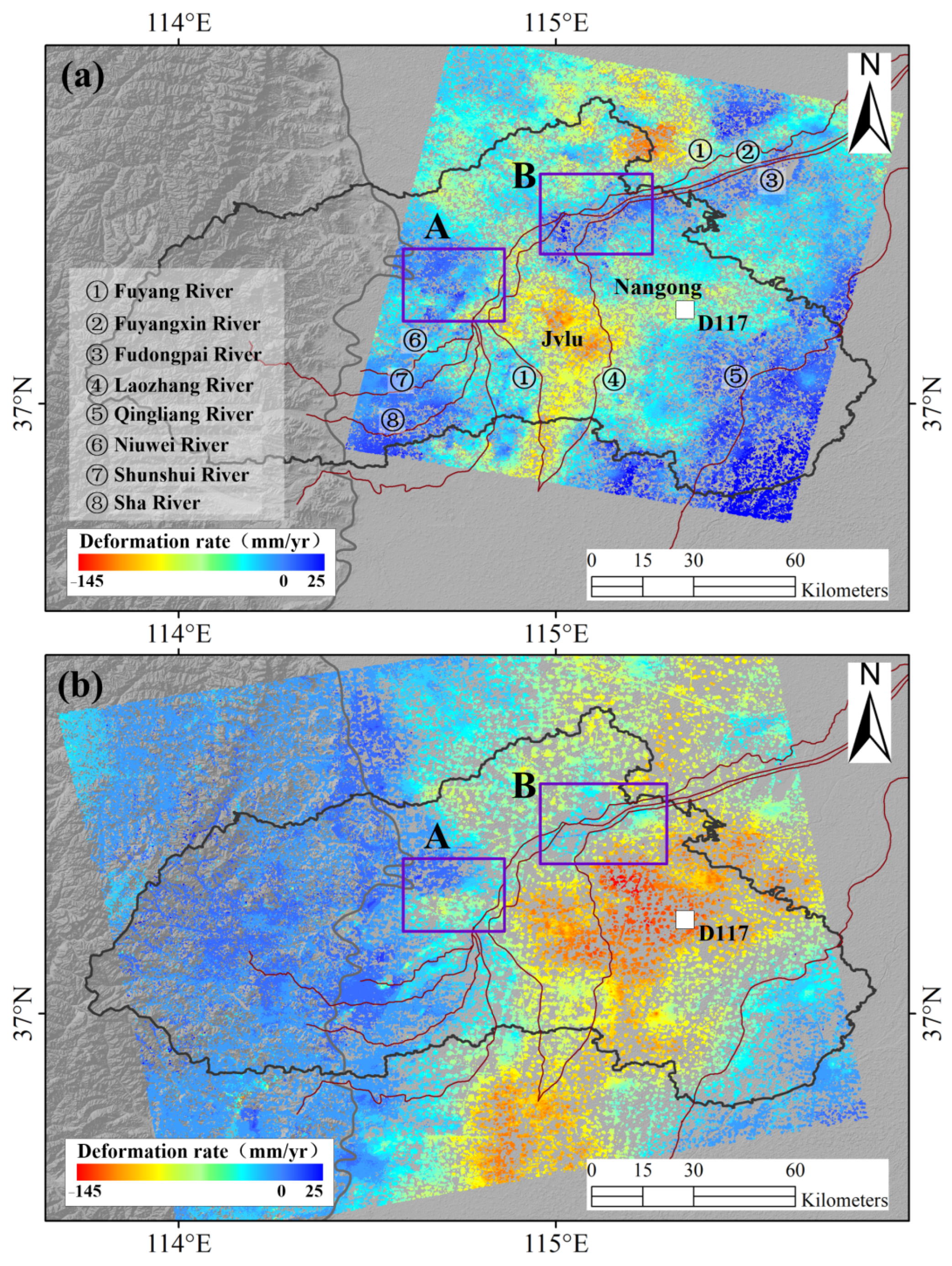
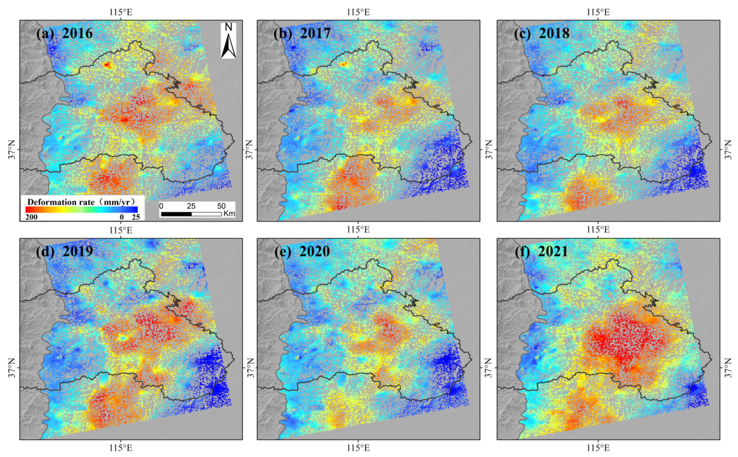
4.1. Spatial and Temporal Variability of Deformation in Xingtai

The maps of the mean deformation rate in Xingtai derived by using Envisat/ASAR data during 2009~2010 and Sentinel-1A data during 2015~2021 are illustrated in Figure 3. The Xingtai plain is dominated by land subsidence, and the extent is controlled by the distribution of the confined aquifers in the west. During 2009~2010, the subsidence patterns were widely found in the plain area of Xingtai, and the most serious subsidence was located in Jvlu with the maximum subsidence rate of 110 mm/year. The subsidence bowl is bounded by the Fuyang River and Laozhang River. Compared with the InSAR-derived subsidence results during 2009~2010, the rate and spatial extent of subsidence increased obviously during 2015~2021. The maximum subsidence rate increased to 140 mm/year, and the subsidence center extended northeastward to Nangong, which is bounded by Fuyang River, Qingliang River and Fudongpai River. An interesting phenomenon is that there is no obvious subsidence (during 2009~2010) or slight subsidence (during 2015~2021) along the Fuyang River, Fuyangxin River and Fudongpai River (Zone B in Figure 3). The most likely reason for this phenomenon is that the rivers decrease the groundwater pumping for irrigation and increase the lateral recharge to the aquifer systems. Additionally, a similar phenomenon can also be found along the Niuwei River and in the area between the Shunshui River and Sha River over the Western Xingtai plain during 2015~2021.
The subsidence is mainly caused by the aquifer system compaction due to groundwater overexploitation [48]. To investigate the response of the aquifer system to head change, we compared the head change at observation well D117 with the mean displacement time series within a 500 m radius around the well (location shown in Figure 3). The hydraulic head at well D117 was approximately stable (less than ±1 m/year) during 2009~2010 and 2016~2017, but subsidence continued at a rapid rate. This suggests that the subsidence is dominated by the inelastic subsidence due to the irreversible compaction in aquitards. Because the hydraulic conductivity of aquitards is low, the response of aquitards lags behind the head change. Thus, we used an exponential decay model of time to characterize the evolution of the delayed subsidence [25,49]: b ( t ) = M ( e k t 1 ) , where b(t) is the time series of displacement, M decreases the magnitude of the subsidence and k is the decay coefficient, which ranges from −1 to 0. A lower k indicates a greater decreasing trend of subsidence rate. The decay coefficients are −0.83 during 2009~2010 and −0.32 during 2015~2017 (Figure 4a,b), suggesting that the relatively static head has obviously slowed down the subsidence. However, no significant decay of subsidence existed during 2015~2021, with a decay coefficient of −0.04. Although the head data were unavailable during 2018~2021, we can infer that the head drops in specific years (e.g., 2019 and 2021) should be responsible for the greater decay coefficient, since the corresponding annual subsidence rate increased significantly (Figure 4b and Figure 5).
The evolution of annual subsidence rate from 2016 to 2021 is shown in Figure 5. The results reveal that the spatial subsidence patterns are similar, but the annual subsidence rate changes greatly from year to year. The average annual subsidence rate in the Xingtai plain was 58 mm/year, 39 mm/year, 45 mm/year, 51 mm/year, 41 mm/year and 77 mm/year from 2016 to 2021, respectively, showing a slight increasing trend. The rate and spatial extent of the subsidence bowl reached the minimum level in 2017, with the maximum subsidence rate being 120 mm/year. The most severe subsidence occurred in 2021, and the subsidence rate reached up to more than 200 mm/year. The amount of groundwater pumping is the major control factor for land subsidence [50]; thus, the rapid subsidence in 2016, 2019 and 2021 should be attributable to the intensive exploitation of groundwater.

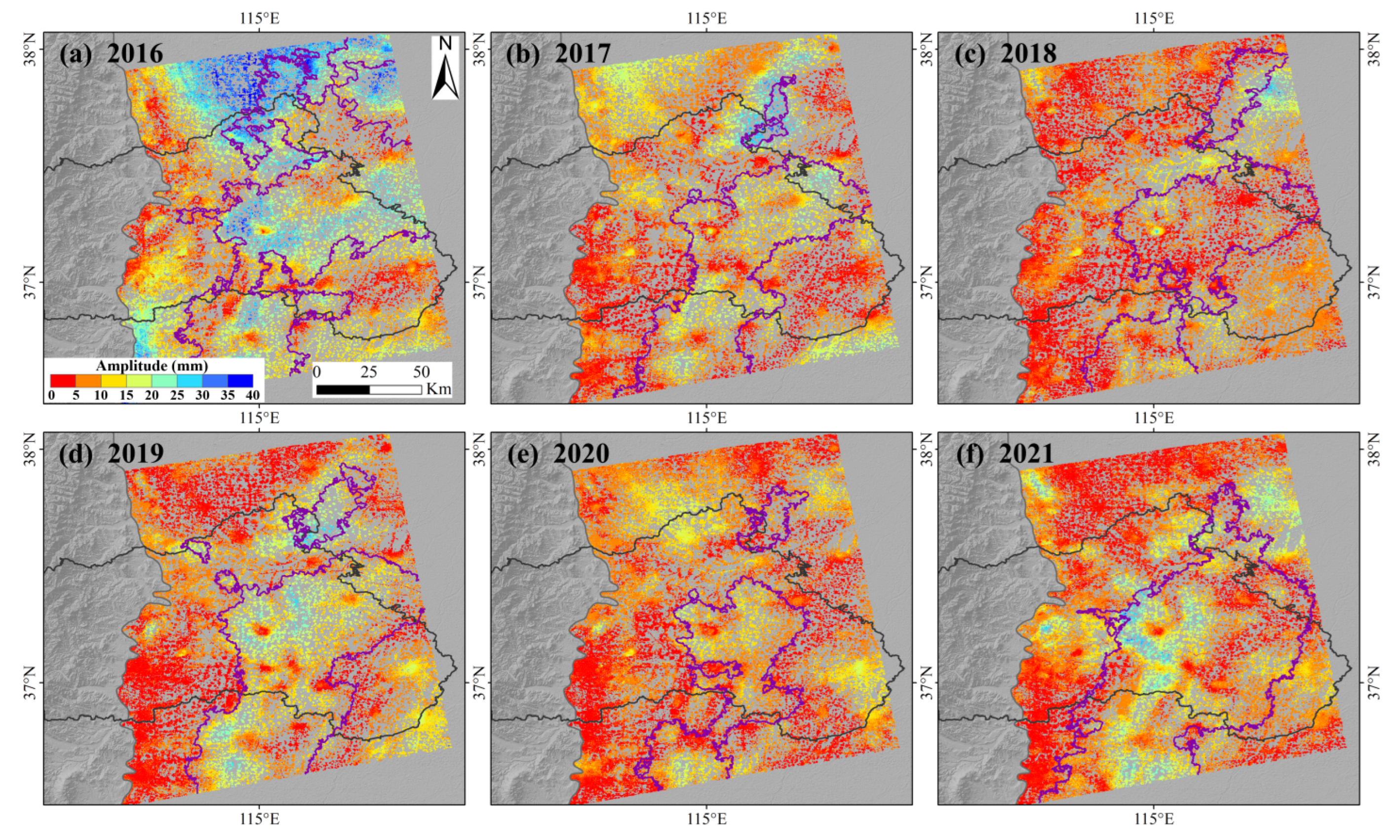
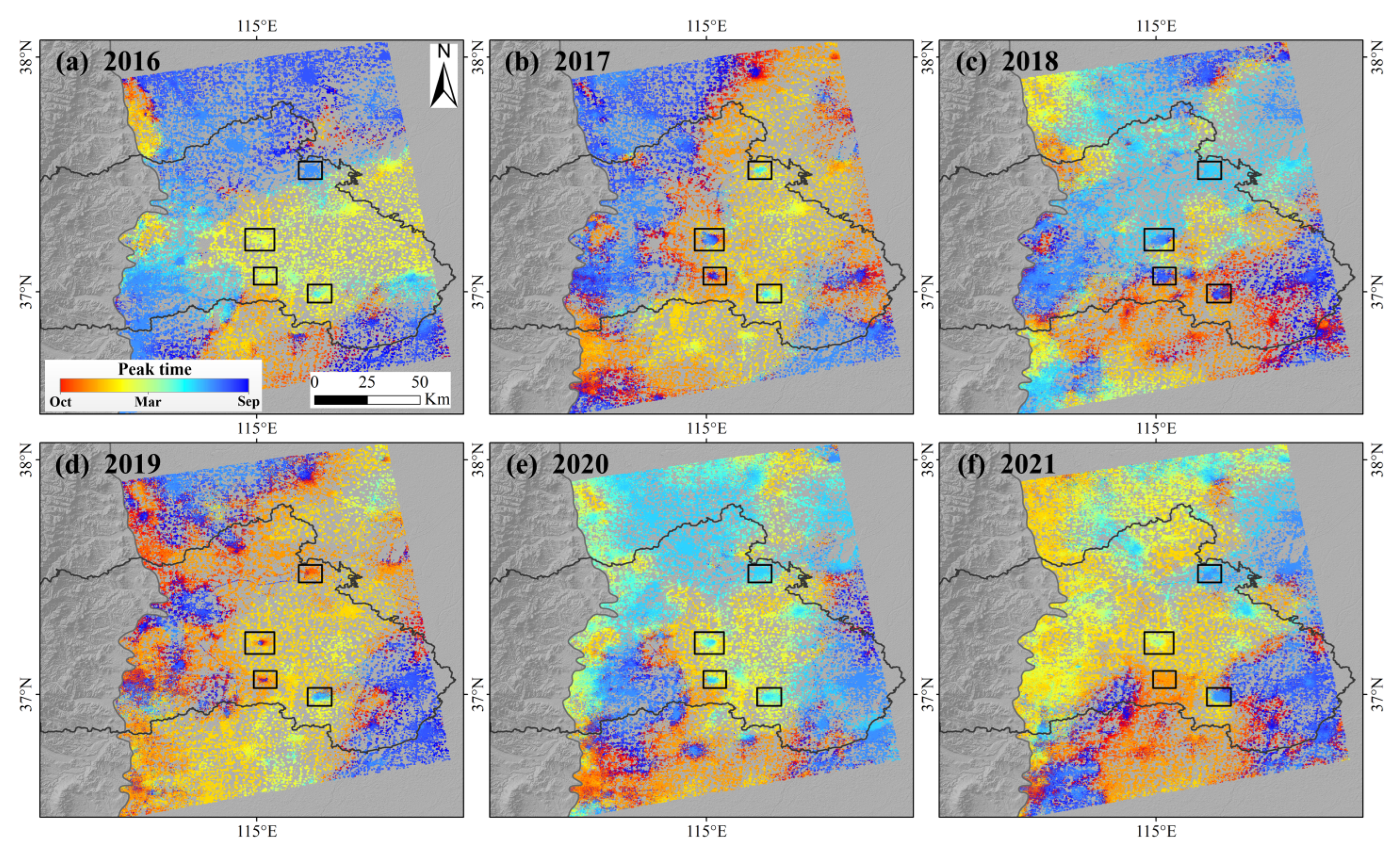
4.2. Amplitude and Timing of Seasonal Deformation

Besides the inelastic deformation, the head change also results in elastic deformation. Figure 4d indicates that the seasonal change in hydraulic head of ~13 m at well D117 leads to seasonal elastic deformation. The amplitude of seasonal deformation is ~20 mm, and the time corresponding to the peak surface uplift is March. Due to the low hydraulic conductivity, the seasonal deformation lags approximately one month behind the seasonal head change (Figure 6a). To investigate the spatial and temporal variability of seasonal deformation, the amplitude and peak time of seasonal deformation across the Xingtai plain in each year during 2016~2021 were estimated by using Equation (1) (Figure 7). Since the period of Envisat/ASAR data was short and too many gaps existed, the seasonal deformation during 2009~2010 was not isolated. The results suggest that the significant seasonal deformation is widely distributed across the Xingtai plain. The amplitude is usually in the range of 0~30 mm and could reach up to 40 mm over the Northern Xingtai plain in 2016. The seasonal deformation with greater amplitude is characterized by a zonal distribution pattern in space. Since the aquifer system is controlled by the distribution of paleochannels [51], the thicker aquifer composed of sand and gravel along the paleochannels results in the larger elastic skeletal storativity. Moreover, because the hydraulic conductivity is relatively higher than that in aquitards, the area with the thicker aquifer is suitable for groundwater exploitation, leading to the larger head changes. The larger elastic skeletal storativity and head changes along the paleochannels should be responsible for the zonal distribution of greater seasonal deformation.
The intensity of groundwater pumping can influence both the annual subsidence rate and seasonal deformation. From Figure 5 and Figure 7, we can see that the distribution of seasonal deformation with greater amplitude (larger than 10 mm) is consistent with that of the rapid subsidence rate (larger than 60 mm/year). Moreover, a high temporal correlation (R = 0.64) is observed between the annual subsidence rate and amplitude of seasonal deformation (Figure 6b), suggesting that their temporal evolutions agree well with each other. The Sentinel-1A data were missing from the period of June to September in 2016, during which the peak/trough deformation occurred; this resulted in relatively larger uncertainty of isolated seasonal deformation. Thus, the results in 2016 were not used in this correlation analysis.
In the natural state, the groundwater is affected by precipitation, and the head reaches the peak value during June~August in each year [52]. However, the head change is controlled by groundwater pumping for agriculture in the irrigation area of Xingtai [53]. The groundwater pumping for irrigation during March~July leads to the head reaching the lowest level in July~August for each year. The leakage recharge from the overlying aquifers and the piedmont lateral recharge both raise the head to the peak level in January~March. From Figure 8, we can know that the peak time across the subsidence center was January~March in all six years, suggesting that the intensity of groundwater-pumping is kept at a high level. This is because that saline unconfined groundwater is distributed in this region; the groundwater is mainly pumped from the confined aquifer system for agricultural demand. In contrast, both the unconfined and confined groundwater are pumped for irrigation in the Northern Xingtai plain. Due to the change of pumping intensity, the peak time in the Northern Xingtai plain varied from June~August in 2016, 2018 and 2020 to January~March in 2017, 2019 and 2021. An interesting phenomenon is that the amplitude of seasonal deformation in the urban areas (black boxes in Figure 8) is relatively small, and the peak time is always June~August. The groundwater in the urban area is used to satisfy the domestic demand; there is no significant seasonal fluctuation in groundwater withdrawal, resulting in the peak head occurring during June~August, similar to the temporal change of head in the natural state. Additionally, the government has restricted the groundwater pumping for domestic use since 2015, causing the smaller amplitude of seasonal deformation. The analysis of this subsection suggests that the subsidence rate, seasonal amplitude and corresponding peak time can be used for investigating the intensity of confined groundwater pumping in areas with head-observation scarcity.

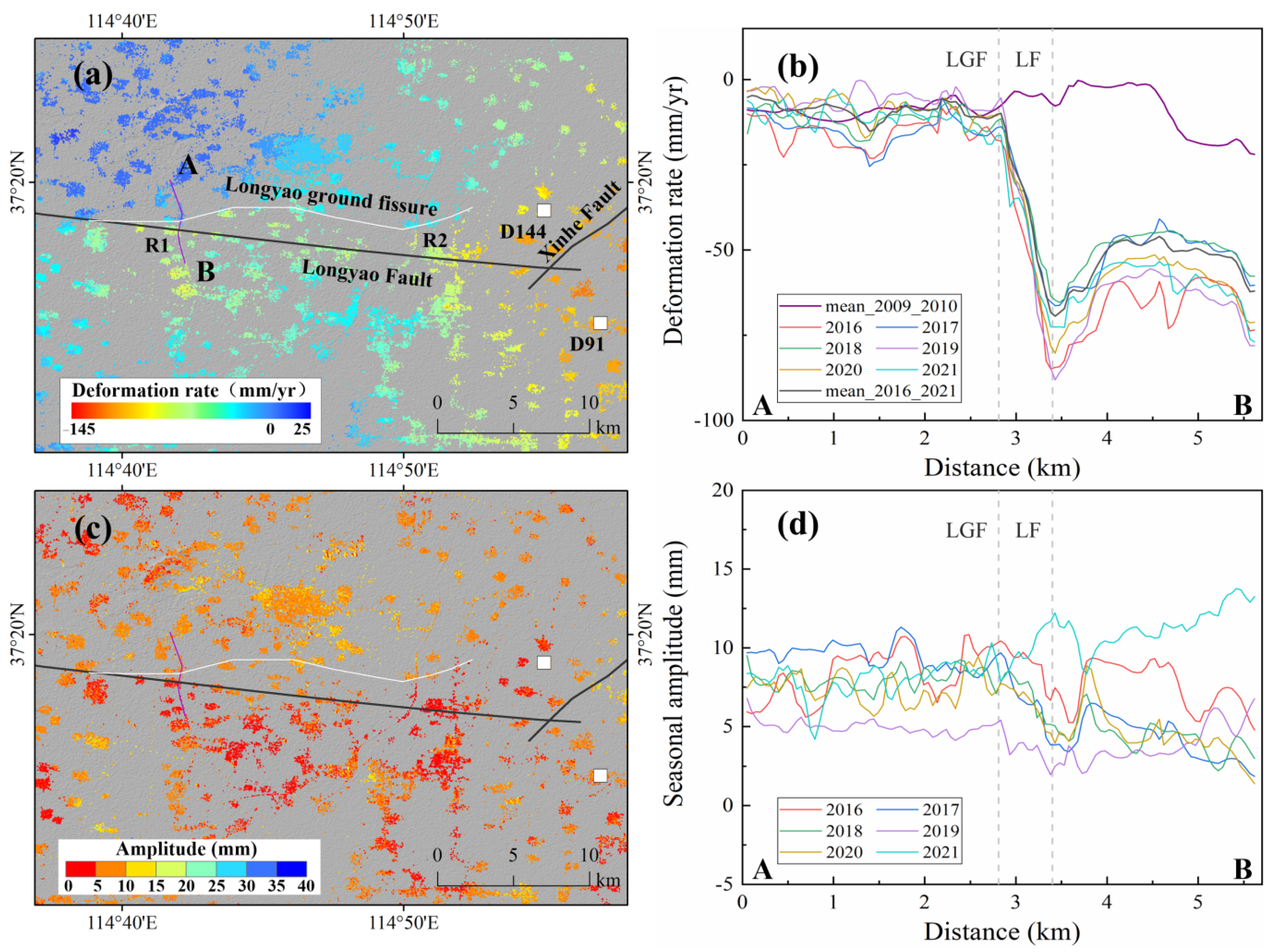
4.3. Activity of Ground Fissure

The fault is filled with poorly permeable fine-grained sediment and acts as a groundwater barrier, which can lead to a head difference between the two sides of a fault. The fault also may cause different aquifer deposits on its two sides, resulting in a difference in aquifer properties. As a result, the deformation difference across a fault will easily occur when groundwater is pumped and further result in a ground fissure. As the most active fissure in the NCP, the Longyao ground fissure’s formation is closely related to the Longyao Fault, and the overexploitation of groundwater plays a key positive role in promoting its activity [6]. Figure 9a shows the detailed distribution of deformation during 2015~2021 in Zone A. It can be found that there are significant changes in the deformation rate between the two sides of the Longyao ground fissure. Obviously, discontinuous deformation rates along linear roads can be found (R1 and R2 in Figure 9a). The profile of deformation rate along R1 across the Longyao ground fissure and Longyao Fault is shown in Figure 9b. During 2015~2021, the deformation rate in the northern part of the ground fissure was relatively stable (less than −10 mm/year), increased sharply between the Longyao ground fissure and Longyao Fault, and reached up to −70 mm/year at the fault location. The maximum deformation rate difference of 80 mm/year between the two sides of fault occurred in 2019. This large gradient of deformation rate difference over the range of ~600 m may result in potential crack initiation. The deformation rate difference between the two sides of the ground fissure was less than 10 mm/year during 2009~2010, inferring that the activity of ground fissure increased significantly during 2015~2021.
The seasonal deformation is also influenced by the Longyao ground fissure and Longyao Fault (Figure 9c,d). The amplitude of seasonal deformation increased or decreased by 3~6 mm between the two sides of the ground fissure during 2016~2021. Thus, the seasonal amplitude can be used to identify the potential fault or ground fissure in the areas where no obvious deformation or head drops occur. According to the difference of deformation rate and seasonal amplitude, we can infer that the western and central sections of the Longyao Fault play roles in preventing the flow of groundwater. However, the time series of the hydraulic head depth at wells located on the two sides of the eastern section of the Longyan Fault and Xinhe Fault show good consistency (Figure 10), suggesting that the aquifer property is homogeneous and the hydraulic connection is good across these two faults in this region.
As mentioned in Section 4.1, the area along the Fuyang River, Fuyangxin River and Fudongpai River was relatively stable during 2009~2010 and 2015~2021. Similar to the spatial deformation pattern surrounding the Longyao ground fissure, a sharp change of deformation rate within a short distance can also be found on the boundaries of the stable area and subsidence bowl (white lines in Figure 11a). The profile of mean deformation rate during 2015~2021 indicates that the deformation rate increased or decreased by 15 mm/year, 22 mm/year and 32 mm/year at lines f1, f2 and f3, respectively (Figure 11b). The annual deformation rates show similar spatial patterns. These large gradients of deformation rate suggest that there might be three unknown fissures at the three lines. The trends of these unknown fissures are roughly consistent with those of the Xinhe Fault. During 2009~2010, the difference of deformation rate of ~10 mm/year occurred at potential fissure f1, and no obvious difference in the deformation rate existed at potential fissures f2 and f3, suggesting that the activities of these unknown fissures increased during 2015~2021. The distribution of amplitude of seasonal deformation is also controlled by the unknown fissures (Figure 11c). The seasonal amplitude changed by 3~8 mm, 3~19 mm and 5~12 mm at three unknown fissures, respectively (Figure 11d). Even if the deformation rate is small, the seasonal amplitude difference of more than 1 cm across the potential fissures might also damage buildings and infrastructures.

4.4. Skeletal Storativity

To estimate the elastic skeletal storativity, we used the harmonic function (Equation (1)) to extract the seasonal head change. Then, combining the isolated seasonal head change and the corresponding seasonal deformation, we estimated the elastic skeletal storativity by using Equation (2). Since no observable seasonal head change occurred at 13 observation wells, the elastic skeletal storativity at 26 well locations was finally estimated. The values of elastic skeletal storativity range from 0.9 × 10⁻³ to 12.4 × 10⁻³. The estimated elastic skeletal storativity shows good consistency with the results of the pumping test, namely 1.0 × 10⁻³ to 8.0 × 10⁻³ [2], except for the value of 12.4 × 10⁻³ at well D103. Compared with the pumping test, the spatial sampling of observation wells is much denser, inferring that our estimation method of skeletal storativity has an advantage by being able to detect the extreme values. The values of elastic skeletal storativity in the Xingtai plain are much larger than those in Cangzhou (0.2 × 10⁻³ to 4.4 × 10⁻³), which is located in the Eastern NCP [50]. This is most likely caused by the thicker aquifers in the Xingtai plain. Figure 12a shows the spatial distribution of estimated elastic skeletal storativity. We find that high values (lager than 4 × 10⁻³) of the elastic skeletal storativity are distributed in the southeastern part of the Xingtai plain.
In the case that the head declines below the pre-consolidation head, the rearrangement of grain in aquitards occurs, leading to inelastic subsidence. In order to estimate the inelastic skeletal storativity, the wells where the head was below the pre-consolidation head and both subsidence and head declines occurred during the study period need to be selected [50]. Based on the analysis of the historical head observations and relationship between head change and deformation, we identified 16 wells to estimate the inelastic skeletal storativity, using Equation (3). The values of inelastic skeletal storativity range from 6.2 × 10⁻³ to 88.0 × 10⁻³, with an average of 31.6 × 10⁻³. The spatial distribution of the estimated inelastic skeletal storativity is illustrated in Figure 12b. The results indicate that the maximum inelastic skeletal storativity is found in the Central Xingtai plain, and the values of inelastic skeletal storativity can vary greatly within a short distance.
Theoretically, the inelastic skeletal storativity is much larger than the elastic skeletal storativity. There are 11 wells where both elastic and inelastic skeletal storativity are estimated. We compared the values of elastic and inelastic skeletal storativity at these 11 well locations (Table 2). The elastic skeletal storativity is less than 30% of the inelastic skeletal storativity, except for the result at well D103. The average value of inelastic skeletal storativity is 5.4 times as much as that of elastic skeletal storativity, inferring that ~84.5% of total subsidence is irreversible and permanent when the head is below the pre-consolidation head.

5. Discussion

In this study, Envisat/ASAR images during 2009–2010 and Sentinel-1 SAR images during 2015–2021 were used to detect the land deformation in the Xingtai plain. However, the parameters of the two SAR datasets are quite different (e.g., incidence angles and orbit direction). The different parameters may have led to uncertainty when we investigated the evolution of vertical land deformation during the two study periods, which were directly converted from the LOS direction, using the incident angle. Previous studies [6,10] pointed out that the horizontal component of deformation is much smaller than the vertical component. The contribution of horizontal deformation to the LOS deformation is negligible. Therefore, the uncertainty due to the different sensor configurations is at an acceptable level, although the parameters are quite different (descending vs. ascending, 22.9° vs. 41.6°).
The spatial distribution of observation wells is sparse (one well per ~220 km2) and uneven, and temporal sampling is low (one time per year during 2009–2010, and 12 times per year) in the Xingtai plain. It is difficult to characterize the spatial and temporal variability of groundwater in detail by using only well observations. By combining InSAR displacement time series and head measurements, we can investigate the response of deformation to head changes at observation wells. Based on the derived coupling relationship, InSAR deformation can be used to characterize the groundwater change in the Xingtai plain with the significantly improved spatial and temporal resolution. To a certain extent, it overcomes the limitation that sparse observation wells cannot characterize detailed regional groundwater change. Therefore, we believe that InSAR will be a useful method for mapping land deformation associated with groundwater withdrawal and investigating confined groundwater change across a basin-wide scale with limited groundwater observations around the world.

6. Conclusions

In this study, we used the StaMPS method with 14 Envisat/ASAR images from 2009 to 2010 and 178 Sentinel-1A images from 2015 to 2021 to detect land deformation in the Xingtai plain. Combining InSAR results, head observations, and geological data, we investigated the spatial–temporal evolution of the deformation and ground fissure and characterized the skeletal storativity in the confined aquifer system. Our conclusions are as follows:
(1).
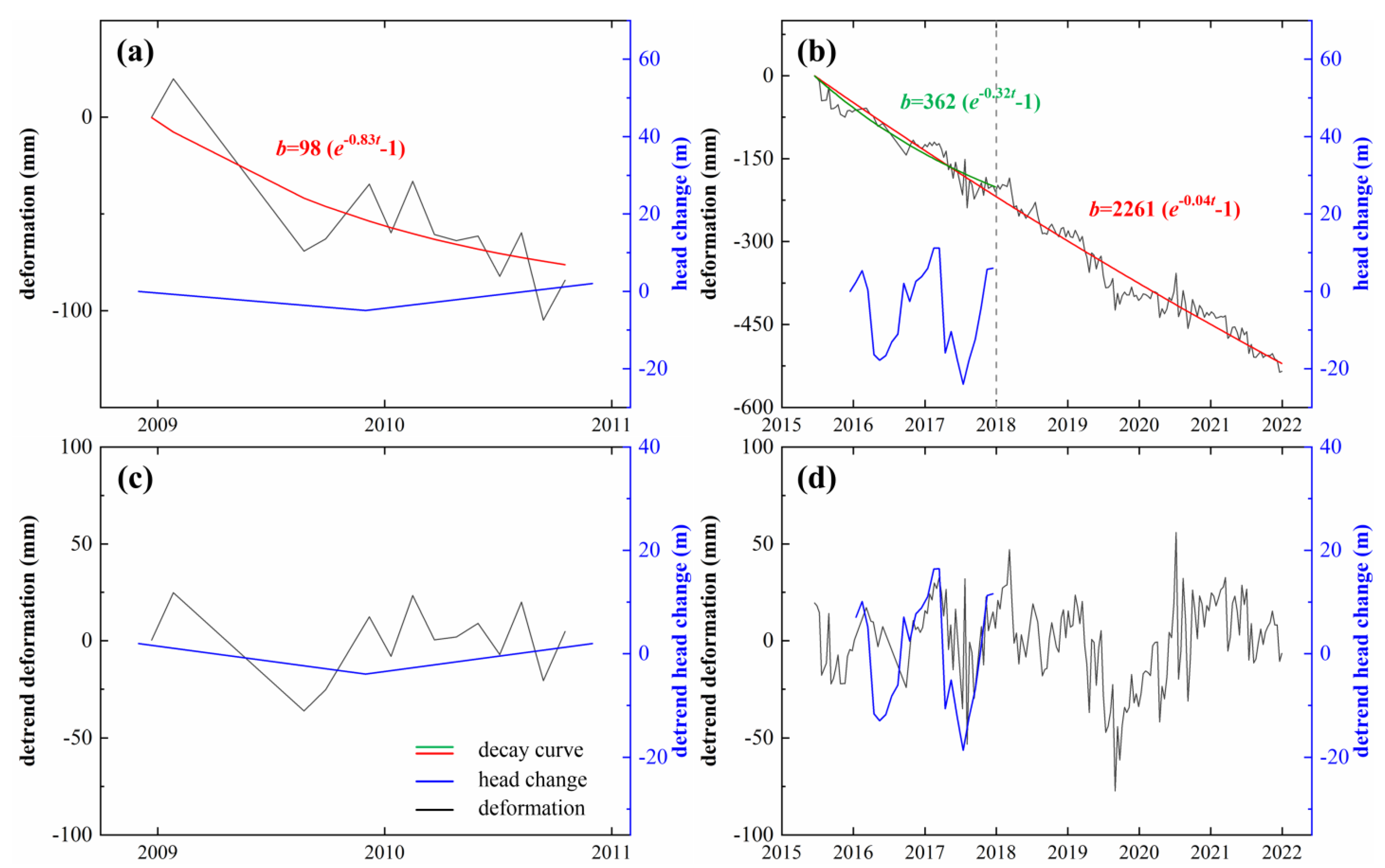
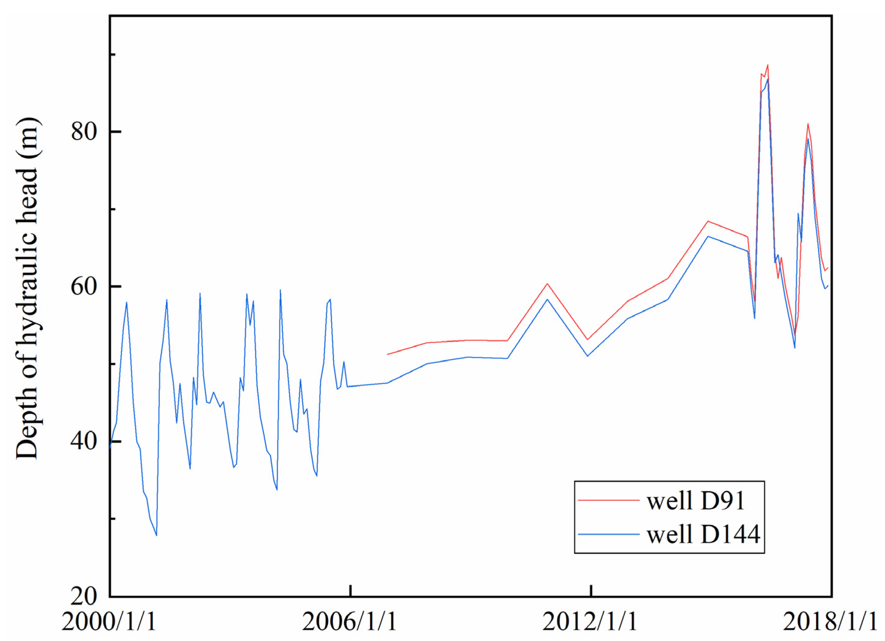
The InSAR-derived results suggest that the Xingtai plain was dominated by land subsidence during the study period. Our joint analysis of displacement time series and head change infers that the subsidence was mainly inelastic, which was caused by the irreversible compaction in aquitards. The relatively static head mitigated subsidence during 2009~2010; however, both the magnitude and spatial extent of subsidence increased obviously during 2015~2021.
(2).
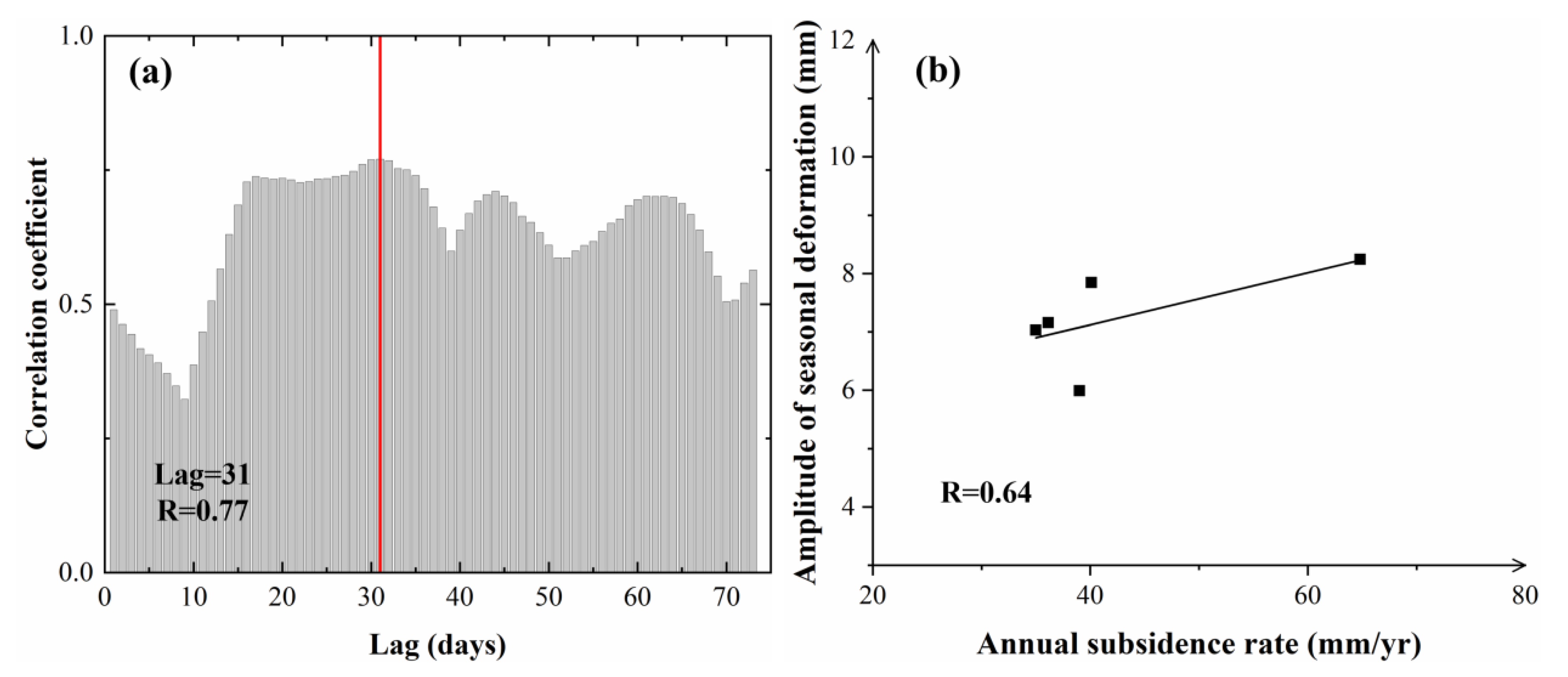
Seasonal fluctuation in hydraulic head resulted in seasonal deformation, with an amplitude of 0~30 mm. The spatial–temporal distribution of seasonal deformation with greater amplitude (larger than 10 mm) is consistent with that of the rapid subsidence (larger than 60 mm/year). The high intensity of groundwater pumping during 2016~2021 led to the peak time of seasonal deformation in the subsidence bowl being in January~March.
(3).
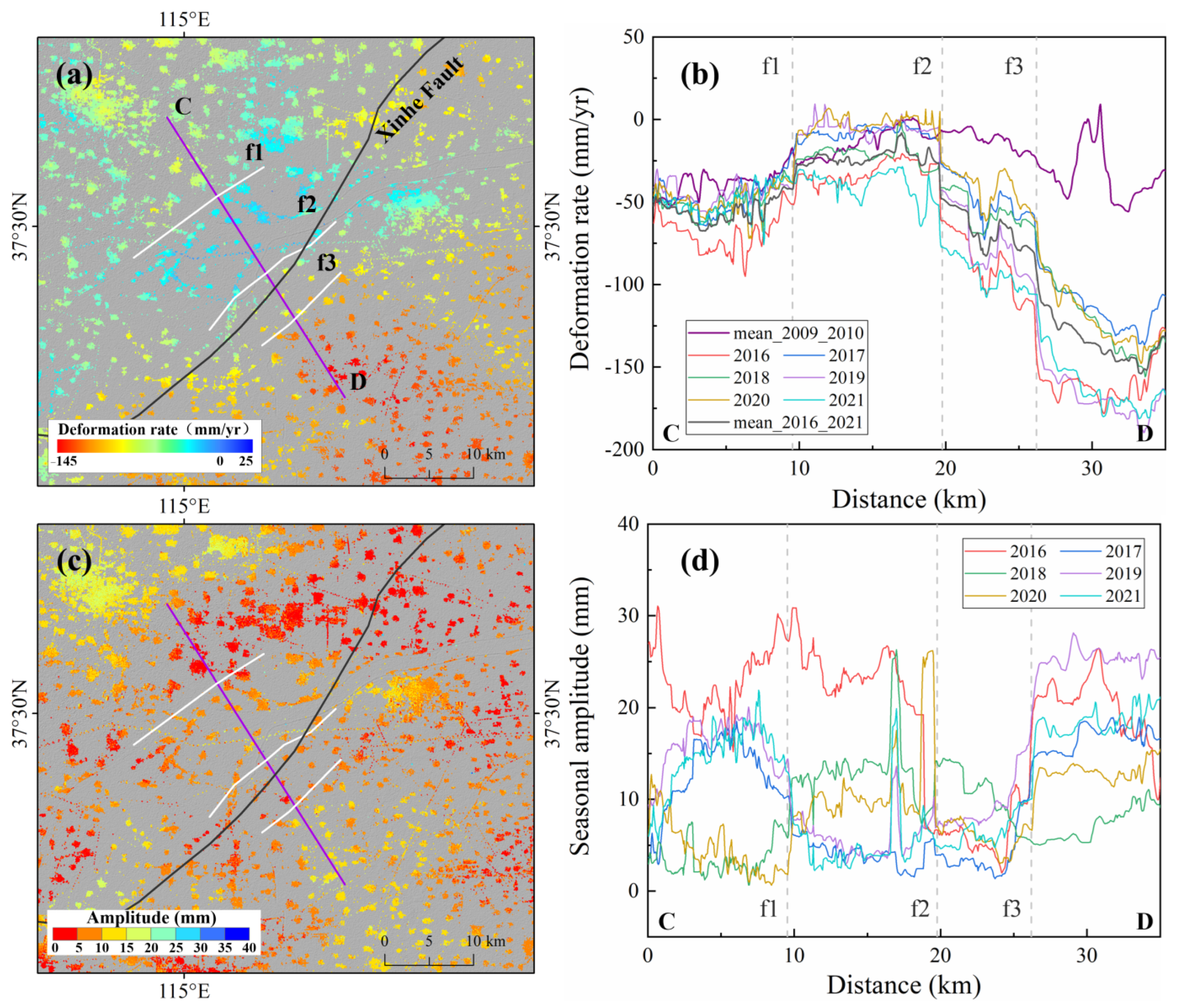
Both the deformation rate and amplitude of seasonal deformation changed greatly across the Longyao ground fissure, with the differences of 70 mm/year and 6 mm, respectively. Then three unknown potential fissures were identified by the large gradients of the deformation rate and seasonal amplitude. Our comparison of the difference in deformation rate and seasonal amplitude during two study periods suggests that the activity of ground fissures during 2015~2021 increased compared with that during 2009~2010.
(4).
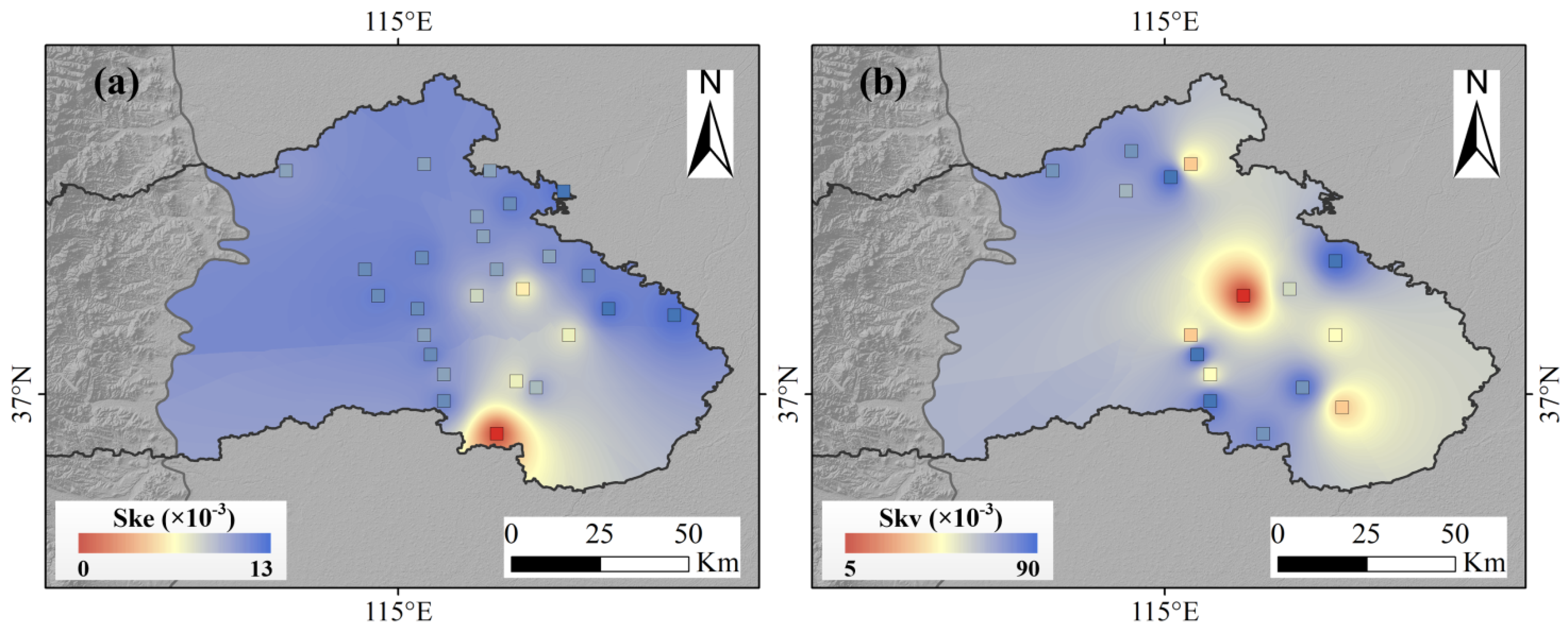
The elastic skeletal storativity at 26 well locations was estimated to be 0.9 × 10⁻³ to 12.4 × 10⁻³, using seasonal deformation and seasonal head change. Based on the inelastic deformation and the long-term components of head change, the inelastic skeletal storativity at 16 well locations was estimated to be 6.2 × 10⁻³ to 88.0 × 10⁻³. The comparison between values of elastic and inelastic skeletal storativity infers that ~84.5% of total subsidence is irreversible and permanent when the head is below the pre-consolidation head.
This study demonstrates that InSAR, with the advantage of a high density of PS pixels, short temporal interval and large coverage, is potentially suitable for characterizing land deformation induced by groundwater overexploitation, detecting potential fissures, investigating confined groundwater change and estimating the skeletal storativity in confined aquifer systems. By combining the multi-sensor InSAR measurements, head observations and estimated aquifer parameters, we can improve the understanding of the coupling relationship between land deformation and head change, further evaluate the confined GWS depletion and provide beneficial suggestions for groundwater monitoring and management.

Author Contributions

Conceptualization, L.B. and S.S.; methodology, L.B.; software, L.B.; validation, S.S. and L.B.; formal analysis, S.S.; investigation, S.S. and L.B.; resources, S.S., L.B. and C.Y.; data curation, S.S.; writing—original draft preparation, S.S.; writing—review and editing, L.B. and C.Y.; visualization, S.S.; supervision, S.S. and L.B.; project administration, L.B.; funding acquisition, L.B. and S.S. All authors have read and agreed to the published version of the manuscript.

Funding

This research was funded by the National Key Research and Development Program of China (Grant No. 2019YFC1509201), the National Natural Science Foundation of China (42004005, 42174032), the Natural Science Basic Research Program of Shaanxi (2021JQ-228) and the Fundamental Research Funds for the Central Universities, CHD (Ref. 300102261105, 300102262205 and 300102262902).

Data Availability Statement

The Envisat/ASAR data are freely available at https://esar-ds.eo.esa.int/oads/access/collection/ (accessed on 14 August 2022). The Sentinel-1A data are freely available at https://scihub.copernicus.eu/dhus/#/home (accessed on 14 August 2022).

Acknowledgments

The authors want to thank ESA for proving the Envisat/ASAR data (projects: Dragon-4 32388 and 32244, Dragon-5 59339 and Data Service Request 37777) and Sentinel-1A data. We also thank Hooper at the University of Leeds for providing the StaMPS software.

Conflicts of Interest

The authors declare no conflict of interest.

References

  1. Hoffmann, J.; Zebker, H.A.; Galloway, D.L.; Amelung, F. Seasonal subsidence and rebound in Las Vegas Valley, Nevada, observed by synthetic aperture radar interferometry. Water Resour. Res. 2001, 37, 1551–1566. [Google Scholar] [CrossRef]
  2. Zhang, Z.; Fei, Y.; Chen, Z.; Zhao, Z.; Xie, Z.; Wang, Y.; Miao, J.; Yang, L.; Shao, J.; Jin, M.; et al. Investigation and Assessment of Sustainable Utilization of Groundwater Resources in the North China Plain; Geological Publishing House: Beijing, China, 2009. (In Chinese) [Google Scholar]
  3. Feng, W.; Zhong, M.; Lemoine, J.M.; Biancale, R.; Hsu, H.T.; Xia, J. Evaluation of groundwater depletion in North China using the Gravity Recovery and Climate Experiment (GRACE) data and ground-based measurements. Water Resour. Res. 2013, 49, 2110–2118. [Google Scholar] [CrossRef]
  4. Jiang, L.; Bai, L.; Zhao, Y.; Cao, G.; Wang, H.; Sun, Q. Combining InSAR and hydraulic head measurements to estimate aquifer parameters and storage variations of confined aquifer system in Cangzhou, North China Plain. Water Resour. Res. 2018, 54, 8234–8252. [Google Scholar] [CrossRef]
  5. Zhu, J.; Guo, H.; Li, W.; Tian, X. Relationship between land subsidence and deep groundwater yield in the North China Plain. South–North Water Transf. Water Sci. Technol. 2014, 12, 165–169. (In Chinese) [Google Scholar] [CrossRef]
  6. Yang, C.; Lu, Z.; Zhang, Q.; Zhao, C.; Peng, J.; Ji, L. Deformation at longyao ground fissure and its surroundings, north China plain, revealed by ALOS PALSAR PS-InSAR. Int. Appl. Earth. Obs. 2018, 67, 1–9. [Google Scholar] [CrossRef]
  7. Long, D.; Yang, W.; Scanlon, B.R.; Zhao, J.; Liu, D.; Burek, P.; Wada, Y. South-to-North Water Diversion stabilizing Beijing’s groundwater levels. Nat. Commu. 2020, 11, 3665. [Google Scholar] [CrossRef]
  8. Pang, B.; Fu, F.; Wang, L. Underground water mining restriction and physical mechanism analysis in Cangzhou. Water Technol. 2014, 8, 45–49. (In Chinese) [Google Scholar]
  9. Guo, H.; Li, W.; Wang, L.; Chen, Y.; Zang, X.; Wang, Y.; Bian, Y. Present situation and research prospects of the land subsidence driven by groundwater levels in the North China Plain. Hydrogeol. Eng. Geol. 2021, 48, 162–171. (In Chinese) [Google Scholar] [CrossRef]
  10. Bai, L.; Li, Z.; Song, S.; Liu, D. Estimation of the land deformation and aquifer parameters in the Handan plain using multi-temporal InSAR technology. Chin. J. Geophys. 2022, 65, 3351–3362. (In Chinese) [Google Scholar] [CrossRef]
  11. Neely, W.R.; Borsa, A.A.; Burney, J.A.; Levy, M.C.; Silverii, F.; Sneed, M. Characterization of groundwater recharge and flow in California’s San Joaquin Valley from InSAR-observed surface deformation. Water Resour. Res. 2021, 57, e2020WR028451. [Google Scholar] [CrossRef]
  12. Gomez-Chova, L.; Fernández-Prieto, D.; Calpe, J.; Soria, E.; Vila, J.; Camps-Valls, G. Urban monitoring using multi-temporal SAR and multi-spectral data. Pattern Recognit. Lett. 2006, 27, 234–243. [Google Scholar] [CrossRef]
  13. Dewan, A.M.; Kankam-Yeboah, K. Using synthetic aperture radar (SAR) data for mapping river water flooding in an urban landscape: A case study of Greater Dhaka, Bangladesh. J. Jpn. Soc. Hydrol. Water Resour. 2006, 19, 44–54. [Google Scholar] [CrossRef]
  14. Hess, L.L.; Melack, J.M.; Filoso, S.; Wang, Y. Delineation of inundated area and vegetation along the Amazon floodplain with the SIR-C synthetic aperture radar. IEEE Trans. Geosci. Remote Sens. 1995, 33, 896–904. [Google Scholar] [CrossRef]
  15. Yusoff, I.M.; Abir, I.A.; Syahreza, S.; Rusdi, M.; Razi, P.; Lateh, H. The applications of InSAR technique for natural hazard detection in smart society. In Journal of Physics: Conference Series; IOP Publishing: Bristol, UK, 2020; Volume 1572. [Google Scholar]
  16. Jiang, M.; Guarnieri, A.M. Distributed scatterer interferometry with the refinement of spatiotemporal coherence. IEEE Trans. Geosci. Remote Sens. 2020, 58, 3977–3987. [Google Scholar] [CrossRef]
  17. Xiao, R.; Jiang, M.; Li, Z.; He, X. New insights into the 2020 Sardoba dam failure in Uzbekistan from Earth observation. Int. Appl. Earth. Obs. 2022, 107, 102705. [Google Scholar] [CrossRef]
  18. Chen, B.; Li, Z.; Zhang, C.; Ding, M.; Zhu, W.; Zhang, S.; Han, B.; Du, J.; Cao, Y.; Zhang, C.; et al. Wide Area Detection and Distribution Characteristics of Landslides along Sichuan Expressways. Remote Sens. 2022, 14, 3431. [Google Scholar] [CrossRef]
  19. Zhang, C.; Li, Z.; Yu, C.; Chen, B.; Ding, M.; Zhu, W.; Yang, J.; Liu, Z.; Peng, J. An integrated framework for wide-area active landslide detection with InSAR observations and SAR pixel offsets. Landslides 2022, 1–19. [Google Scholar] [CrossRef]
  20. Bai, L.; Jiang, L.; Wang, H.; Sun, Q. Spatiotemporal characterization of land subsidence and uplift (2009–2010) over wuhan in central china revealed by terrasar-X insar analysis. Remote Sens. 2016, 8, 350. [Google Scholar] [CrossRef]
  21. Hooper, A.; Bekaert, D.; Spaans, K.; Arıkan, M. Recent advances in SAR interferometry time series analysis for measuring crustal deformation. Tectonophysics 2012, 514, 1–13. [Google Scholar] [CrossRef]
  22. Kumar, H.; Syed, T.H.; Amelung, F.; Agrawal, R.; Venkatesh, A.S. Space-time evolution of land subsidence in the national capital region of India using ALOS-1 and sentinel-1 SAR data: Evidence for groundwater overexploitation. J. Hydrol. 2022, 605, 127329. [Google Scholar] [CrossRef]
  23. Orhan, O. Monitoring of land subsidence due to excessive groundwater extraction using small baseline subset technique in Konya, Turkey. Environ. Monit. Assess. 2021, 193, 174. [Google Scholar] [CrossRef] [PubMed]
  24. Li, M.; Sun, J.; Xue, L.; Shen, Z.; Zhao, B.; Hu, L. Characterization of Aquifer System and Groundwater Storage Change Due to South-to-North Water Diversion Project at Huairou Groundwater Reserve Site, Beijing, China, Using Geodetic and Hydrological Data. Remote Sens. 2022, 14, 3549. [Google Scholar] [CrossRef]
  25. Chaussard, E.; Bürgmann, R.; Shirzaei, M.; Fielding, E.; Baker, B. Predictability of hydraulic head changes and characterization of aquifer-system and fault properties from InSAR-derived ground deformation. J. Geophys. Res. Solid Earth 2014, 119, 6572–6590. [Google Scholar] [CrossRef]
  26. Hoffmann, J.; Galloway, D.L.; Zebker, H.A. Inverse modeling of interbed storage parameters using land subsidence observations, Antelope Valley, California. Water Resour. Res. 2003, 39, 1031. [Google Scholar] [CrossRef]
  27. Miller, M.M.; Shirzaei, M. Spatiotemporal characterization of land subsidence and uplift in Phoenix using InSAR time series and wavelet transforms. J. Geophys. Res. Solid Earth 2015, 120, 5822–5842. [Google Scholar] [CrossRef]
  28. Ojha, C.; Shirzaei, M.; Werth, S.; Argus, D.F.; Farr, T.G. Sustained groundwater loss in California’s Central Valley exacerbated by intense drought periods. Water Resour. Res. 2018, 54, 4449–4460. [Google Scholar] [CrossRef]
  29. Liu, P.; Yang, C.; Zhao, C. PS-InSAR monitoring of Longyao ground fissure in Xingtai, Hebei province. Shanghai Land Resour. 2017, 38, 78–82. (In Chinese) [Google Scholar] [CrossRef]
  30. Li, X.; Yan, L.; Lu, L.; Huang, G.; Zhao, Z.; Lu, Z. Adjacent-Track InSAR Processing for Large-Scale Land Subsidence Monitoring in the Hebei Plain. Remote Sens. 2021, 13, 795. [Google Scholar] [CrossRef]
  31. Cao, R. Study on Dynamic Evaluation Model and System of Groundwater Pressure Extraction Effect in Xingtai City. Ph.D. Thesis, Xi’an University of Technology, Xi’an, China, 2021. (In Chinese). [Google Scholar]
  32. The People’s Government of Xingtai City. Available online: http://www.xingtai.gov.cn/mlxt/xtgk/201912/t20191227_553585.html (accessed on 14 August 2022).
  33. Department of Natural Resources of Hebei Province, Bulletin of Geological Environment of Hebei Province in 2015, Shijiazhuang, China. 2016. Available online: http://info.hebei.gov.cn/eportal/ui?pageId=6778557&articleKey=6786172&columnId=330104 (accessed on 7 September 2022). (In Chinese)
  34. Ma, X.J.; Song, W.; WANG, H.L. Causes for the ground cleave in Longyao county. J. Geol. Hazards Environ. Preserv. 2011, 22, 43–47. [Google Scholar]
  35. Chen, T. Study on the optimization adjustment of karst water protection zones in Xingtai. Master’s Thesis, China University of Geosciences (Beijing), Beijing, China, 2021. (In Chinese). [Google Scholar]
  36. Hooper, A. A multi-temporal InSAR method incorporating both persistent scatterer and small baseline approaches. Geophys. Res. Lett. 2008, 35, L16302. [Google Scholar] [CrossRef]
  37. Hooper, A.; Segall, P.; Zebker, H. Persistent scatterer interferometric synthetic aperture radar for crustal deformation analysis, with application to Volcán Alcedo, Galápagos. J. Geophys. Res. Solid Earth 2007, 112, B07407. [Google Scholar] [CrossRef]
  38. Hooper, A.; Zebker, H.; Segall, P.; Kampes, B. A new method for measuring deformation on volcanoes and other natural terrains using InSAR persistent scatterers. Geophys. Res. Lett. 2004, 31, L23611. [Google Scholar] [CrossRef]
  39. Yu, C.; Li, Z.; Penna, N.T.; Crippa, P. Generic atmospheric correction model for interferometric synthetic aperture radar observations. J. Geophys. Res. Solid Earth 2018, 123, 9202–9222. [Google Scholar] [CrossRef]
  40. Yu, C.; Penna, N.T.; Li, Z. Generation of real-time mode high-resolution water vapor fields from GPS observations. J. Geophys. Res. Atmos. 2017, 122, 2008–2025. [Google Scholar] [CrossRef]
  41. Xiao, R.; Yu, C.; Li, Z.; He, X. Statistical assessment metrics for InSAR atmospheric correction: Applications to generic atmospheric correction online service for InSAR (GACOS) in Eastern China. Int. J. Appl. Earth Obs. Geoinf. 2021, 96, 102289. [Google Scholar] [CrossRef]
  42. Hooper, A.; Zebker, H.A. Phase unwrapping in three dimensions with application to InSAR time series. JOSA A 2007, 24, 2737–2747. [Google Scholar] [CrossRef]
  43. Hu, X.; Lu, Z.; Wang, T. Characterization of hydrogeological properties in salt lake valley, Utah, using InSAR. J. Geophys. Res. Earth Surf. 2018, 123, 1257–1271. [Google Scholar] [CrossRef]
  44. Riley, F.S. Analysis of borehole extensometer data from central California. Land Subsid. 1969, 2, 423–431. [Google Scholar]
  45. Leake, S. Interbed storage changes and compaction in models of regional groundwater flow. Water Resour. Res. 1990, 26, 1939–1950. [Google Scholar] [CrossRef]
  46. Riel, B.; Simons, M.; Ponti, D.; Agram, P.; Jolivet, R. Quantifying ground deformation in the Los Angeles and Santa Ana Coastal Basins due to groundwater withdrawal. Water Resour. Res. 2018, 54, 3557–3582. [Google Scholar] [CrossRef]
  47. Miller, M.M.; Shirzaei, M.; Argus, D. Aquifer mechanical properties and decelerated compaction in Tucson, Arizona. J. Geophys. Res. Solid Earth 2017, 122, 8402–8416. [Google Scholar] [CrossRef]
  48. Xu, J.; Peng, J.; Ma, X.; Ma, R.; Yang, X.; Feng, S.; An, H. Characteristic and mechanism analysis of ground fissures in Longyao, Xingtai. J. Eng. Geol. 2012, 20, 160–169. [Google Scholar]
  49. Hu, X.; Xue, L.; Yu, Y.; Guo, S.; Cui, Y.; Li, Y.; Qi, S. Remote Sensing Characterization of Mountain Excavation and City Construction in Loess Plateau. Geophys. Res. Lett. 2021, 48, e2021GL095230. [Google Scholar] [CrossRef]
  50. Bai, L.; Jiang, L.; Zhao, Y.; Li, Z.; Cao, G.; Zhao, C.; Liu, R.; Wang, H. Quantifying the influence of long-term overexploitation on deep groundwater resources across Cangzhou in the North China Plain using InSAR measurements. J. Hydrol. 2022, 605, 127368. [Google Scholar] [CrossRef]
  51. Investigation Report of Groundwater Resources Assessment and Rational Development & Utilization in Hebei Plain (Heilonggang Area); Hebei Bureau of Geology and Mineral Resources Exploration: Shijiazhuang, China, 1977. (In Chinese)
  52. Fu, D. Dynamic Characteristics of Groundwater Level in Handan, Hebei Plain Area. Master’s Thesis, Shijiazhuang University of Economics, Shijiazhuang, China, 2013. (In Chinese). [Google Scholar]
  53. Ge, Y. Environmental Investigation and Comprehensive Evaluation of Typical Groundwater Sources in Xingtai City. Master’s Thesis, Qingdao University, Qingdao, China, 2021. (In Chinese). [Google Scholar]
Figure 1. Map of study area in the NCP. The gray line highlights the extent of Xingtai. Observation wells are shown with white squares. The purple rectangles mark the coverage of Envisat/ASAR and Sentinel-1A SAR datasets. The blue line marks the Fuyang River. The brown line shows the boundary of the NCP. The green lines represent the contours of the sand content. The white lines represent the faults.
Remotesensing 14 04488 g001
Figure 2. Temporal/perpendicular baselines of (a) Envisat/ASAR and (b) Sentinel-1A interferometric pairs.
Remotesensing 14 04488 g002
Figure 3. The mean-deformation-rate maps over Xingtai during (a) 2009~2010 and (b) 2015~2021. The brown lines mark the rivers. The white squares represent observation well, of which displacement time series is compared with head changes in Figure 4. The purple boxes, labeled as A and B, mark the zones which are analyzed in Section 4.3.
Remotesensing 14 04488 g003
Figure 4. Comparison between mean displacement time series (gray line) for pixels within a 500 m radius around well D117 and head changes (blue line) during (a) 2009–2010 and (b) 2015–2021. Comparison between de-trended deformation (gray line) and de-trended head changes (blue line) during (c) 2009–2010 and (d) 2015–2021. The red and green lines represent the decay curve estimated by using the exponential decay model of time.
Remotesensing 14 04488 g004
Figure 5. The maps of annual deformation rate over Xingtai plain in (af) 2016~2021.
Remotesensing 14 04488 g005
Figure 6. (a) Correlation analysis between the de-trend displacement and the de-trend head time series at observation well D117. The red line marks the highest correlation coefficient. (b) Comparison between annual subsidence rate and amplitude seasonal deformation.
Remotesensing 14 04488 g006
Figure 7. The amplitude of seasonal deformation across the Xingtai plain in (af) 2016~2021.The purple lines mark the contours of a subsidence rate of 60 mm/a.
Remotesensing 14 04488 g007
Figure 8. The peak time of seasonal deformation across the Xingtai plain in (af) 2016~2021. The black boxes mark the county’s urban areas.
Remotesensing 14 04488 g008
Figure 9. (a) The map of InSAR-derived land deformation rate during 2015~2021 in Zone A. (b) The profile of deformation rate across the Longyao ground fissure and Longyao Fault during 2009~2010 and 2016–2021. (c) The map of amplitude of seasonal deformation in 2018 over Zone A. (d) The profile of amplitude of seasonal deformation along the line of AB during 2016–2021. The purple line marks the profile line, the white line represents the Longyao ground fissure, the black lines mark the faults, and the white squares represent the observation wells.
Remotesensing 14 04488 g009
Figure 10. Time series of the depth of hydraulic head at wells D91 and D144 during 2000~2017.
Remotesensing 14 04488 g010
Figure 11. (a) The map of InSAR-derived land deformation rate during 2015~2021 in Zone B. (b) Profile of deformation rate along line of CD during 2009~2010 and 2016–2021. (c) The map of amplitude of seasonal deformation in 2020 in Zone B. (d) Profile of amplitude of seasonal deformation along line of CD during 2016–2021. The purple line marks the profile line, the white lines represent the potential fissures and the black line marks the fault.
Remotesensing 14 04488 g011
Figure 12. The spatial distribution of estimated (a) elastic and (b) inelastic skeletal storativity, using hydraulic head observations and InSAR derived displacement time series during 2016~2017. The squares mark the observation wells used to estimate skeletal storativity.
Remotesensing 14 04488 g012
Table 1. The parameters of SAR datasets used in this study.
ParametersEnvisat/ASARSentinel-1A
Track no.49040
Orbit directionDescendingAscending
PolarizationVVVV
Band/wavelength (cm)C/5.6C/5.6
Imaging modesIMIW
Incidence angle (degree)22.941.6
Acquisition dates20081222–2010101820150617–20211230
No. of images14178
Table 2. Comparison between values of elastic and inelastic skeletal storativity.
No.Name S k e   ( 10 3 ) S k v   ( 10 3 ) S k e / S k v   ( % )
1D932.3950.634.7
2D961.546.1525.1
3D971.649.4417.3
4D984.2788.024.9
5D992.7647.395.8
6D1006.2534.3118.2
7D1023.0911.2627.4
8D10312.4417.9669.3
9D1045.4446.4111.7
10D1322.6419.1413.8
11D1422.1254.933.9
Publisher’s Note: MDPI stays neutral with regard to jurisdictional claims in published maps and institutional affiliations.

