
Satellite Fog Detection at Dawn and Dusk Based on the Deep Learning Algorithm under Terrain-Restriction

1
School of Geosciences and Info-Physics, Central South University, Changsha 410083, China
2
National Satellite Meteorological Center, China Meteorological Administration, Beijing 100081, China
*
Author to whom correspondence should be addressed.
Remote Sens. 2022, 14(17), 4328; https://doi.org/10.3390/rs14174328
Submission received: 30 June 2022
/
Revised: 27 August 2022
/
Accepted: 29 August 2022
/
Published: 1 September 2022
(This article belongs to the Special Issue Remote Sensing for Climate Change)
Abstract
:Fog generally forms at dawn and dusk, which exerts serious impacts on public traffic and human health. Terrain strongly affects fog formation, which provides a useful clue for fog detection from satellite observation. With the aid of the advanced Himawari-8 imager data (H8/AHI), this study develops a deep learning algorithm for fog detection at dawn and dusk under terrain-restriction and enhanced channel domain attention mechanism (DDF-Net). The DDF-Net is based on the traditional U-Net model, with the digital elevation model (DEM) data acting as the auxiliary information to separate fog from the low stratus. Furthermore, the squeeze-and-excitation networks (SE-Net) is integrated to optimize the information extraction for eliminating the influence of solar zenith angles (SZA) on the spectral characteristics over a large region. Results show acceptable accuracy of the DDF-Net. The overall probability of detection (POD) is 84.0% at dawn and 83.7% at dusk. In addition, the terrain-restriction strategy improves the results at the edges of foggy regions and reduces the false alarm rate (FAR) for low stratus. The accuracy is expected to be improved when training at a season or month scale, rather than at a longer temporal scale. Results of our study help to improve the accuracy of fog detection, which could further support the relevant traffic planning or healthy travel.
1. Introduction
Fog refers to the suspension of microscopic water droplets in the atmosphere [1]. Besides during the night, solar radiation is also weak during the dawn and dusk, resulting in a relatively high probability of fog formation because of the low surface air temperature and high vapor saturation [2]. The dense fog seriously reduces horizontal visibility, which adversely affects public traffic and human health (particularly in rush hours at dawn and dusk) [3]. In addition, anthropogenically generated chemicals dissolve in the foggy water, which would strongly worsen air pollution [4]. Therefore, fog detection at dawn and dusk is crucial to effectively support traffic planning and to provide information and bulletins for reducing risks to human health [5].
Traditional terrestrial fog detection mainly relies on meteorological observation stations. However, it is difficult to be applied at a large-scale due to the limited spatial and temporal resolutions. With the high temporal resolution and spatial continuity observation, satellite remote sensing shows great potential for fog detection on a large scale [6]. Physically, the satellite fog detection algorithm follows the fact that the emissivity of opaque water clouds is lower in the mid-infrared (MIR) band than that in the thermal infrared (TIR) band [7]. Based on this theory, Eyre et al. [8] used the 3.7 μm and 11 μm brightness temperature (BT) of the Advanced Very High-Resolution Radiometer (AVHRR) to identify the nighttime fog and low stratus. Considering the great difference of the dual-channel brightness temperature difference (BTD) between fog, surface and clouds, the BTD is widely used in nighttime fog detection [9,10,11,12,13,14]. However, the method is only suitable for fog detection at nighttime, for which it is difficult to isolate the fog and low stratus (FLS) simultaneously [15]. The MIR band is affected by the solar radiation reflection of the target in the daytime, which causes the dual-channel differential separation detection threshold to vary with the solar zenith angle (SZA) [2]. At dawn and dusk, the MIR reflection is relatively weak due to the high SZA. In regions near to the terminator, the BTD between the fog and surface is similar or consistent, resulting in large uncertainty in fog detection. Gurka et al. [16] analyzed the fog dissipation process and its correlation with the thickness of the fog layer based on the visible light (VIS) band of the Synchronous Meteorological Satellite (SMS-1). Rao et al. [17] discussed the feasibility of identifying FLS in the VIS band of 0.64 μm. At present, the daytime fog detection algorithms are mainly based on the threshold of the spectral and textural differences between cloud, fog, and surface in the 0.67 μm, 3.7 μm, and 11 μm bands [18,19]. However, the MIR and VIS bands are affected by the high SZA at dawn and dusk and the spectral characteristics difference is weak between fog and surface, leaving low confidence in fog detection at dawn and dusk. Using the difference of BTD and reflectivity at 0.67 μm, Yoo et al. [5] proposed a FLS detection algorithm at dawn based on the Communication, Ocean and Meteorological Satellite (COMS) and Fengyun-2D (FY-2D) satellite. However, the method is difficult to monitor fog areas in real-time due to the low temporal resolution of the polar-orbiting satellites. Yang et al. [20] used the geostationary Fengyun-4A (FY-4A) and Himawari-8 (H8) with a higher temporal resolution to retrieve the probability index of Japan/surrounding FLS at dawn, which provides a methodological reference for fog detection at dawn and dusk.
The algorithms mentioned above mainly rely on the spectral difference between fog and other ground objects. Surface environments (particularly the terrain) also strongly affect fog formation and detection [21], which are lacking in most previous algorithms. In general, fog forms near the ground, while clouds form at high altitudes [22]. Furthermore, the edge of fog is restricted by terrain [13], which presents unique spatial variation, vertical structure, and optical properties. By adding terrain information to the fog detection algorithm, it is expected to further improve the accuracy of fog detection. For example, Shang et al. [22] combined DEM with traditional cloud/haze detection indicators to improve the accuracy of cloud, haze, and clear recognition. However, the terrain features of fog classification are the same as the edge elevation of objects, while the spectral features of remote sensing images are mainly at pixel scale. Therefore, it is difficult to fuse the two features in traditional fog detection methods.
The deep learning approach realizes the mapping of input data to detection target results (that is, the detection of fog) through a series of data transformations (layers), replacing the complex multi-stage process with a simple, end-to-end learning model. By using a series of nonlinear functions, the deep learning model describes and classifies the characteristics of the targets [23], which provides a potentially efficient way for fog detection at dawn or dusk. Based on the U-Net model, Jacob et al. [24] proposed an RS-Net cloud detection algorithm that effectively improved the efficiency of cloud detection. Wu et al. [25] proposed a geographic information-driven network (GeoInfo-Net) for cloud and snow detection. In addition to using remote sensing data, the network would encode the auxiliary data sets of the elevation, latitude, and longitude information for network training, which helps to improve the accuracy significantly. However, fog detection is sensitive to the remote sensing bands under different terrain conditions and SZA, resulting in various weight values of each band during deep learning. Meanwhile, fog is a small probability event. The model training strategy needs to be adjusted to speed up the convergence process of model training and avoid overfitting. The problems above leave great uncertainty for the application of deep learning in satellite fog detection. These problems can be optimized by improving the application of the deep learning model. For example, the sensitivity of different SZA and terrain conditions to fog detection can be effectively alleviated by introducing the Squeeze-and-Excitation Networks (SE-Net), which could automatically obtain the weights of the contributions of the parameters [26]. Uneven distribution of training data samples can be solved through the batch normalization of input data. Additionally, the training process could be optimized by designing the independent adaptive learning rates for different parameters and by using efficient optimization algorithms [27]. However, the relevant research is still rare, thus further investigation is warranted.
This study aims to develop a deep learning-based algorithm for satellite fog detection under the terrain-restriction. The DEM data is added into the information input layer to distinguish fog and low cloud. Furthermore, the Squeeze-and-Excitation Networks (SE-Net) is integrated to optimize the model’s information extraction to eliminate the influence of different SZA over a large region. Finally, a deep learning fog detection algorithm under terrain constraints and enhanced channel domain attention mechanism (DDF-Net) is developed for fog detection at dawn and dusk. This study is organized as follows: Section 2 describes the study area, data, details regarding pre-processing methodologies, and the realization of the algorithm. Section 3 includes the results of quantitative and qualitative validation. Finally, the performance and limitation of the DDF-Net are concluded and discussed in Section 4.
2. Materials and Methods
2.1. Study Area and Data Sources
Figure 1 shows an overview of the study area, which is located in northern China (104°30′E~136°00′E and 33°00′N~47°30′N). The western part of the study area includes the Inner Mongolia Plateau and Loess Plateau, with an average altitude of more than 1500 m. The eastern of the study area is located in the third step of the flat terrain of the Chinese topographic demarcation line, where the average altitude drops to 500–1000 m. The study area is located in the eastern of the Henhe-Tengchong Line and has a developed economy and large population. The climate is characterized by a rich source of water vapor from the Western Pacific, which helps to form fog for more than 30 days per year [28]. The frequent fog at dawn and dusk exerts a serious impact on local traffic, especially aviation and highways, and also the economic development and people’s physical and mental health [29].
- (1)
- Satellite data
We adopt the Advanced Himawari-8 Imager (AHI) data with a temporal resolution of 10 min for the investigation. The data set has 16 channels ranging from 0.47 μm to 13.3 μm, with the details could be seen in ref [30]. By referencing the previous studies [22,31,32,33], we select the data sets of bands 3, 5, 6, 7, 11, 13, and 14 for model training and validation. AHI data in foggy days from November to December during 2015~2017 are selected to build 3122 fog mask images (size: 256 × 256) and then divided into 70% for training and 30% for validating.
- (2)
- Ground observation data
The ground observation data was used to execute and validate the algorithm, these data were available from the China Meteorological Administration ground observation stations. The data include observations 8 times per day: 02:00 local time (LT), 05:00 LT, 08:00 LT, 11:00 LT, 14:00 LT, 17:00 LT, 20:00 LT, and 23:00 LT. Among them, the data at 8:00 and 17:00 are used to evaluate the accuracy of the algorithm. The climate would be marked as foggy when the “visibility” is less than 1 km in most criteria. In this study, we followed the criteria and classified the fog as strong, dense and hazy as visibility ranges between 0~200, 200~500 and 500~1000 m, respectively. Meanwhile, the China Meteorological Administration (CMA) promulgated the national standard of Grade of fog forecast (GB/T 27964-2011GB/T) [34], which also defined haze when the horizontal visibility ranges from 1.0 to 10.0 km. Furthermore, it is less harmful to traffic when the visibility is greater than 3 km. Therefore, we defined the haze as visibility ranges from 500~3000 m.
- (3)
- Terrain data
The terrain data used in this study came from the SRTM1-DEM data with a spatial resolution of 30 m released by the United States Geological Survey (USGS). To match the spatial resolution of the H8/AHI data, the DEM data was resampled to 2 km.
2.2. Deep Learning Algorithm
Deep learning realizes the mapping of input data to target results through a series of data transformations (layers) (Figure 2). The basic principle is to output the image as a target result according to the mapping function f of the initial network model [23]. The model compares the prediction with the truth, and then adjusts the parameters and weights through an iterative method to capture the optimal prediction result. The components of the deep learning model generally include the mapping function f, convolutional layers (CL) and pooling layers (PL) [23]. Specifically, f defines the functional relationship between the input x and the target mask classification map y; CL uses a specified number of convolution kernels in each layer to extract the feature information of each pixel of x. The shallow layer includes the textural and spectral features that are used as the basis classification, and the deeper layer represents the higher-level semantics, which is the feature information obtained after several convolutions (feature extraction) [35]. The PL is implemented to sample the channel feature information downward, which divides the input image into several rectangular areas to get the maximum value of each sub-area. Through this way, it will continuously reduce the spatial size of the data, which could reduce the parameters and improve the computation speed [23]. Furthermore, the PL can ensure that the network continuously extracts and utilizes the information through the multi-layer structure of biological neurons. The activation function (Relu) is located between the CL and the PL, which is used to achieve nonlinear transformation. The sigmoid function maps the output of the last CL to values from 0 and 1, and then realizes the classification of the input x for each pixel by setting an appropriate threshold.
In the execution of the deep learning model, the target probability is generated according to the last CL and the sigmoid function. It is defined as the target pixel when the probability is greater than a certain threshold. The deviation between the actual fog coverage and the predicted target mask is calculated using a binary cross-entropy loss function, and the parameter gradient of the mapping function f is calculated and updated by the Backpropagation algorithm (BP) [36] until the optimal parameters of the model are obtained. Specifically, the actual fog coverage is generated by the combination of visual interpretation and ground observation, which is used as the label data for training or validating the algorithm.
2.3. The SE-Net Module
The output of the CL does not consider the dependencies of each channel. SE-Net allows the network to selectively enhance features and suppress useless features. We choose to adopt this approach in our study. The SE-Net module contains 1 global average pooling operation (GP), 2 small fully connected layers (FC), 1 Sigmoid function and 1 channel weighted operation, with the details could be seen in ref [26]. Specifically, the Global pooling (GP) refers to the average of all the pixels of the feature map on each channel. The FC includes two sub-modes of FC1 and FC2. FC1 consists of fully-connected layers with C/16 filters, which is calculated by the weighted summation to reduce the number of parameters and improve the calculation efficiency. The activation function (Relu) is located between the FC1 and the FC2, which is used to achieve nonlinear transformation. FC2 consists of fully-connected layers with C filters, which assure the same numbers of outputs and channels. Finally, the sigmoid normalizes these learned weights to be between 0–1 for dimensionless processing of different features.
Execution steps of the SE-Net module are as follows:
(1) Obtaining the global information from the feature channels. The information of the DEM-AHI fog image at dawn and dusk is extracted through the CL formed by C convolution kernels, and image X with a characteristic channel number of C is formed. Cp is calculated by GP in each feature channel of the image X (Equation (1)):
where Cp is the global information of the feature channel p after GP, W and H are the length and width of the image X, respectively, xp (i,j) represents the pixel value of X at point (i,j) in channel p.
(2) Calculating the correlation between each feature channel. According to the calculated correlation results, the weight of the feature channel that improves the accuracy is increased, while the suppressed or ineffective feature channel’s weight is decreased (Equation (2)):
where F_P_F1 is the feature of output channel p after FC1 and Relu activation function, the FC1 is the first fully connected layer [23,26], the size of F_P_F1 is C/16 × 1 × 1.
(3) Calculate the weight of each feature channel. The Sigmoid function is used to calculate the weight factor Wp of the channel p (Equation (3)):
where the FC2 is the second fully connected layer. Wp represents the weight factor of channel p after function calculation of FC2 and Sigmoid function.
(4) Attention learning of channels. The weighted attention feature is acquired through the weight factor Wp and the pixel value xp of X at channel p (Equation (4)):
The represents the attention feature of channel p learned by SE-Net.
2.4. Deep Learning-Based Algorithm of Fog Detection under Terrain Restriction
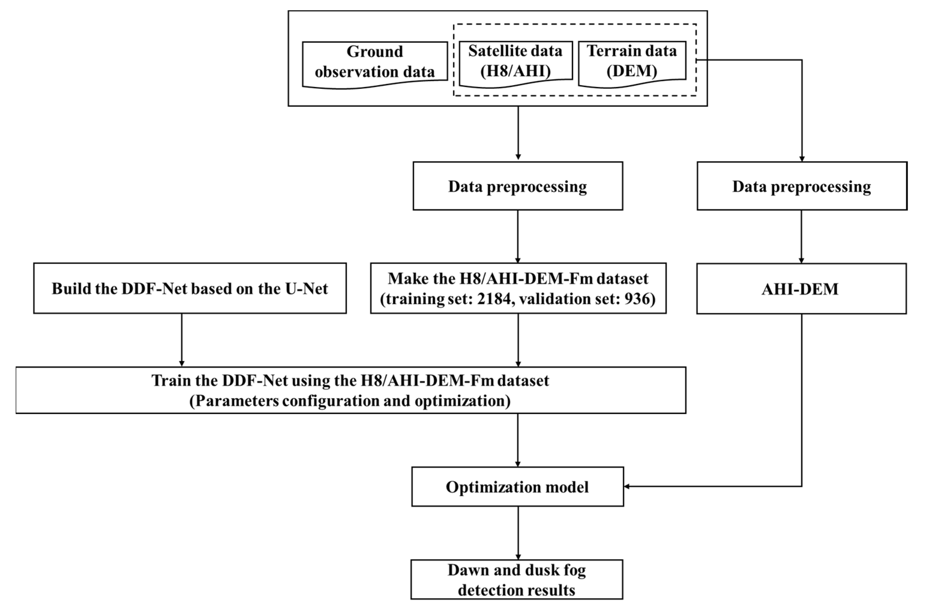
The spatio-spectral characteristics of fog, medium/high clouds and surfaces provide the physical basis for the algorithm of fog detection, while the weak solar radiation severely hinders the separation of fog from the surface and clouds at dawn and dusk. The U-net model had been proven to be a robust and effective method due to its excellent performance and transferability in image segmentation [24,37], which is used as the basic model in our algorithm. Furthermore, terrain strongly affects the formation and movement of fog [21], which should be taken into consideration in the algorithm of fog detection. To overcome these challenges above, this study develops a deep learning-based algorithm for satellite fog detection at dawn and dusk under terrain constraints. The improvement of our method refers to the adaptive algorithm under different SZA and terrain conditions by introducing channel attention mechanisms and adding DEM data to remote sensing images. Specifically, our method extracts fog from the AHI-DEM datasets by integrating the SE-Net module in the CL of the U-net model. Figure 3 depicts the flowchart of the algorithm. The inputs include the ground observation data, satellite data of H8/AHI (bands 3, 5, 6, 7, 11, 13, and 14) and the terrain data (DEM), while the outputs refer to spatial coverage of fog detection under different times.
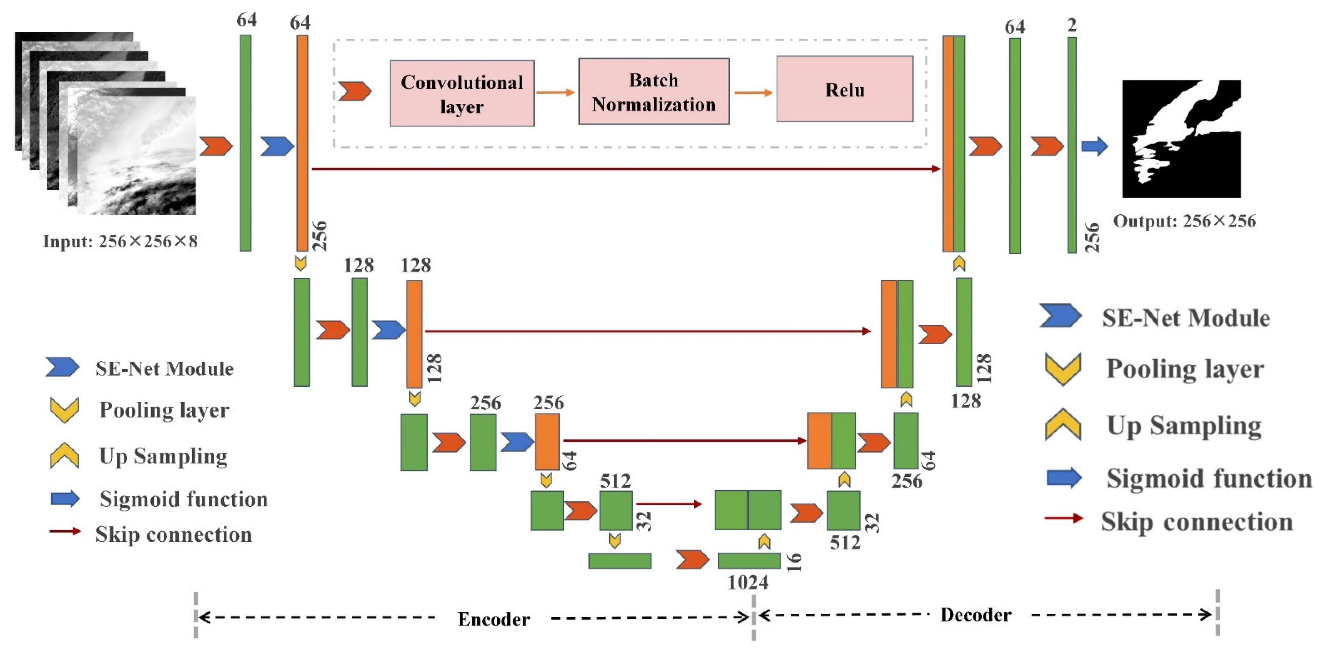
The main structure of the DDF-Net is shown in Figure 4. The input side includes 5 CL, 4 PL and 3 SE-Net modules. The CL can extract the feature information of fog, cloud and surface at dawn or dusk through designing different numbers of 3 × 3 convolution kernel. The BN operation is executed to normalize the input data and the Relu function acts by increasing the model’s ability to fit nonlinear relationships. The PL selects the maximum value of the 4 pixels to reduce the dimension of the feature information and complete the down-sampling of the feature map, which can reduce the parameters and accelerate the training process of the model. The output side includes 4 CL and 4 up-sampling layers. The up-sampling layer restores the dimension of the feature map by duplicating each pixel in the feature map as 4 pixels, which generates less local information in the feature map. Alternatively, the skip connection fuses the feature map to establish a contextual feature information connection and compensate local information, which helps to obtain the semantic space context information of the model [37]. The DDF-Net model composed of these multi-layer structures can approximately fit all complex functions. This is very beneficial to our research, because the state of fog is quite different under different terrains and SZA.
2.4.1. Building the H8/AHI-DEM-Fm Fog Mask Dataset
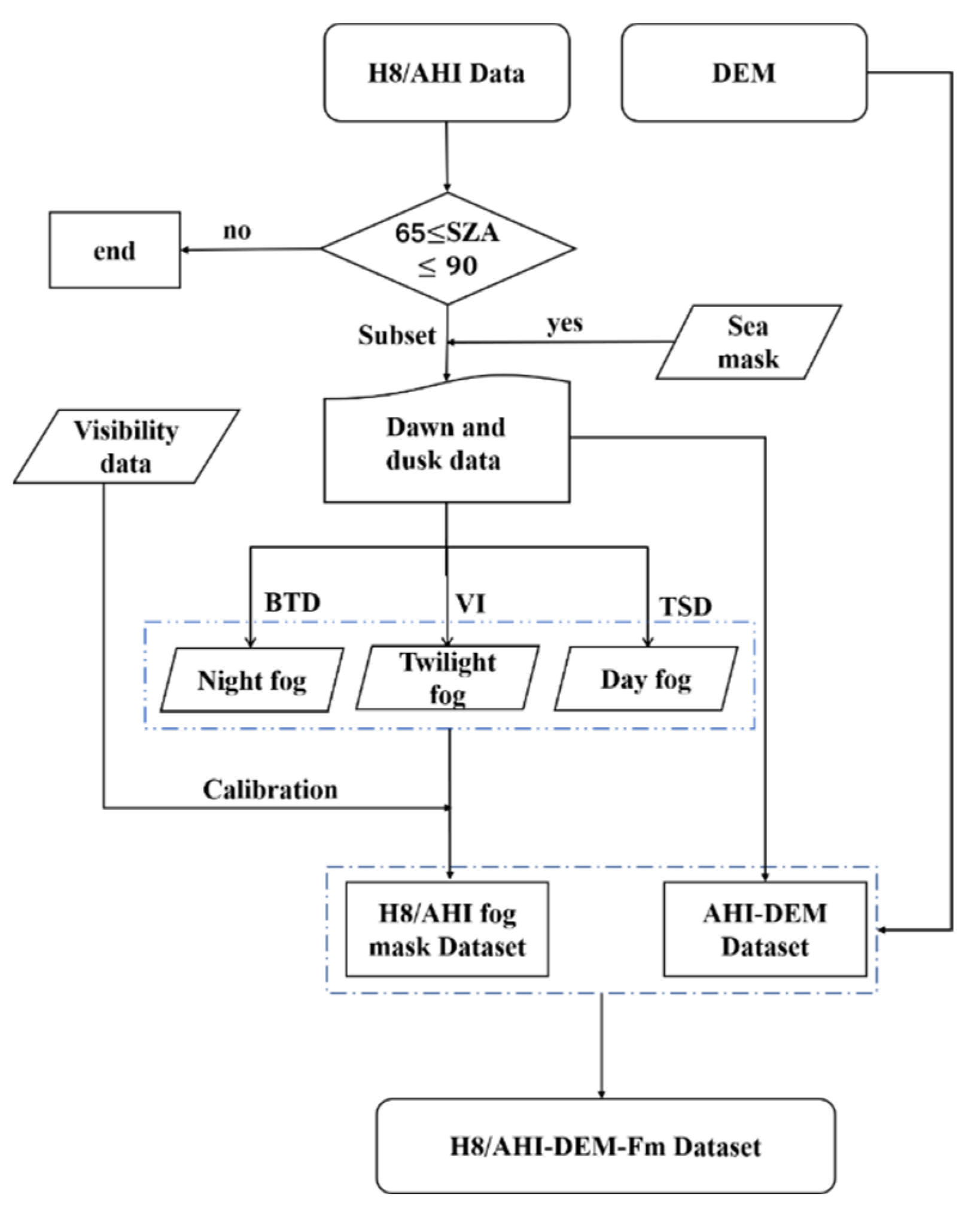
Based on the H8/AHI data, this study firstly builds the training data set (Figure 5). The DEM data was added to the AHI data to refine the model’s detection accuracy at the edge of the foggy area. Fog pixels are labeled by the spectral, textural and movement characteristics of fog, surface and cloud.
- (1)
- Building the AHI-DEM dataset at dawn and dusk.
The remote sensing images including dawn and dusk are screened according to the SZA. Meanwhile, band clipping and sea-land mask clipping are performed. The DEM is combined with AHI data as a channel to construct the AHI-DEM dataset containing the time of dawn and dusk.
- (2)
- Building the fog mask dataset Fm.
The fog pixels marked on the AHI-DEM data are used to build the fog mask data Fm. The pixels are marked as daytime, nighttime and twilight fog through the textural and spectral difference (TSD), bright temperature difference (BTD) and visual interpretation (VI). TSD refers to the differences in the texture spectrum of daytime fog, clouds, and surfaces. The BTD of fog is lower than surfaces and medium/clouds at nighttime. The criterion of VI is that the fog has the characteristics of spatial and temporal consistency within the adjacent 30 min. According to the labeling of the image at the previous moment, it is determined whether there are fog pixels at the current moment. VI is mainly used to identify fog that is similar or consistent with surface spectral information at dawn and dusk. Meanwhile, the ground observation data is used to strictly calibrate the Fm.
- (3)
- Building the H8/AHI-DEM-Fm fog mask dataset.
AHI-DEM and Fm are simultaneously cropped into sub-images of 256 × 256 sizes with 30% overlap to improve the training efficiency of the model and the ability to capture edge information. Finally, H8/AHI-DEM-Fm is produced through the above process.
2.4.2. Integration of the SE-Net Module
SZA strongly affects the fog spectral characteristics, even with the same remote sensing band. For example, the VIS band has a strong effect on the low SZA regions (due to fog being more reflective than the surface and less reflective than clouds), while it is ineffective in the nighttime regions. Therefore, the influence of each band on fog detection under different SZA should be taken into account, which is very important for large-scale dawn and dusk fog detection. Meanwhile, the terrain strongly affects the fog formation and development, which would act as one of the key parameters of fog detection [21]. The SE-Net module can automatically learn the weight of each band in the fog detection task at different conditions of SZA terrain in a data-driven manner, which shows the great potential for fog detection under different SZA.
Assuming that X is the feature map of the c channel output by the Relu function of a certain layer in the encoder, then X can be expressed as:
SE-Net automatically learns the weights W of feature maps on each channel by training:
Finally, the feature map output by SE-net can be expressed as:
The SE-Net module is embedded after the first three Relu (rather than after each Relu in the encoder) to further improve the extraction of fog information under different terrain and SZA conditions, and also avoids the introduction of too many parameters to slow down the model training.
2.4.3. Adjust the Training Strategy of the Model
To optimize the network model, the Adam gradient descent algorithm (Adam) [27,38,39] and BN [40] are introduced to adjust the training strategy. The Adam is introduced to speed up the training process of the model by automatically obtaining the direction of optimized parameters [27,38,39]. The BN is embedded after each CL to normalize the input data to overcome the sudden change in the distribution of a certain batch of training data (Figure 4). In addition, it can also improve the training speed and shortens the training time [38]. The configuration parameters (such as software, graphics card, programming framework, etc.) are shown in Table 1.
(1) By setting the initial parameters of the model (Table 1), the encoder extracts the feature map of the input image. Batch size represents the number of images inputted to the network during model training. Epoch represents the maximum number of rounds of model iteration. αinitial indicates the initial learning rate. Decaying Epoch indicates that the model adjusts the learning rate dynamically according to formula (8) after the studies number of Epoch minus Decaying Epoch.
(2) The decoder combines high-level semantic and low-level spatial information to complete the initial classification of pixels. The model finally outputs the binary result of 0 (non-fog) and 1 (fog). Then, the error between the predicted result and the actual fog coverage is calculated (Equations (9)–(11)). BP assigns the error to each parameter and the Adam is used to update the parameters by using the learning rate provided by the model.
(3) Processes 1–2 are iterated until the indicators are no longer significantly changing and fluctuate around a certain value.
(4) The new remote sensing data are input to the trained DDF-Net model to realize fog detection over the whole study area. The performance of the algorithm could be finally evaluated with the aid of ground observation.
2.5. Evaluation Metrics
This study adopts several metrics to evaluate the accuracy of the training model and the performance accuracy of our algorithm, which are described as follows:
- (1)
- Model Evaluation Metrics
We use the metric of semantic segmentation [33,37], namely Accuracy (Acc), F1-Score (F1) and Intersection-over-Union (IoU) to evaluate the accuracy of the training model. Each indicator is defined as follows:
where Acc is the ratio of the number of correctly classified pixels (Ncorrect) to the total number of pixels in the scene (Ntotal). p represents the proportion of the Ncorrect to the sum of Ncorrect and the number of falsely classified pixels (Nfalse), r represents the proportion of the Ncorrect to the total number of pixels that are foggy in the corresponding label of the images (Nground-truth). IoU represents the ratio of fog pixels in the image predicted by the model to the sum of total number of pixels that are foggy in the corresponding label of the images (Nground-truth) and Nfalse. All indicators are scaled from 0 to 1, the larger the IoU, the higher the segmentation accuracy.
- (2)
- Quantitative evaluation metrics of fog detection accuracy
The probability of detection (POD), false alarm ratio (FAR) and critical success index (CSI) [11] are used for the validation of fog detection, which are described as follows:
where NH, NM and NF are the pixel numbers of hitting, missing and false fog detections. All indicators are scaled from 0 to 1, with high POD and CSI and low FAR indicating great performance of the algorithm.
3. Results
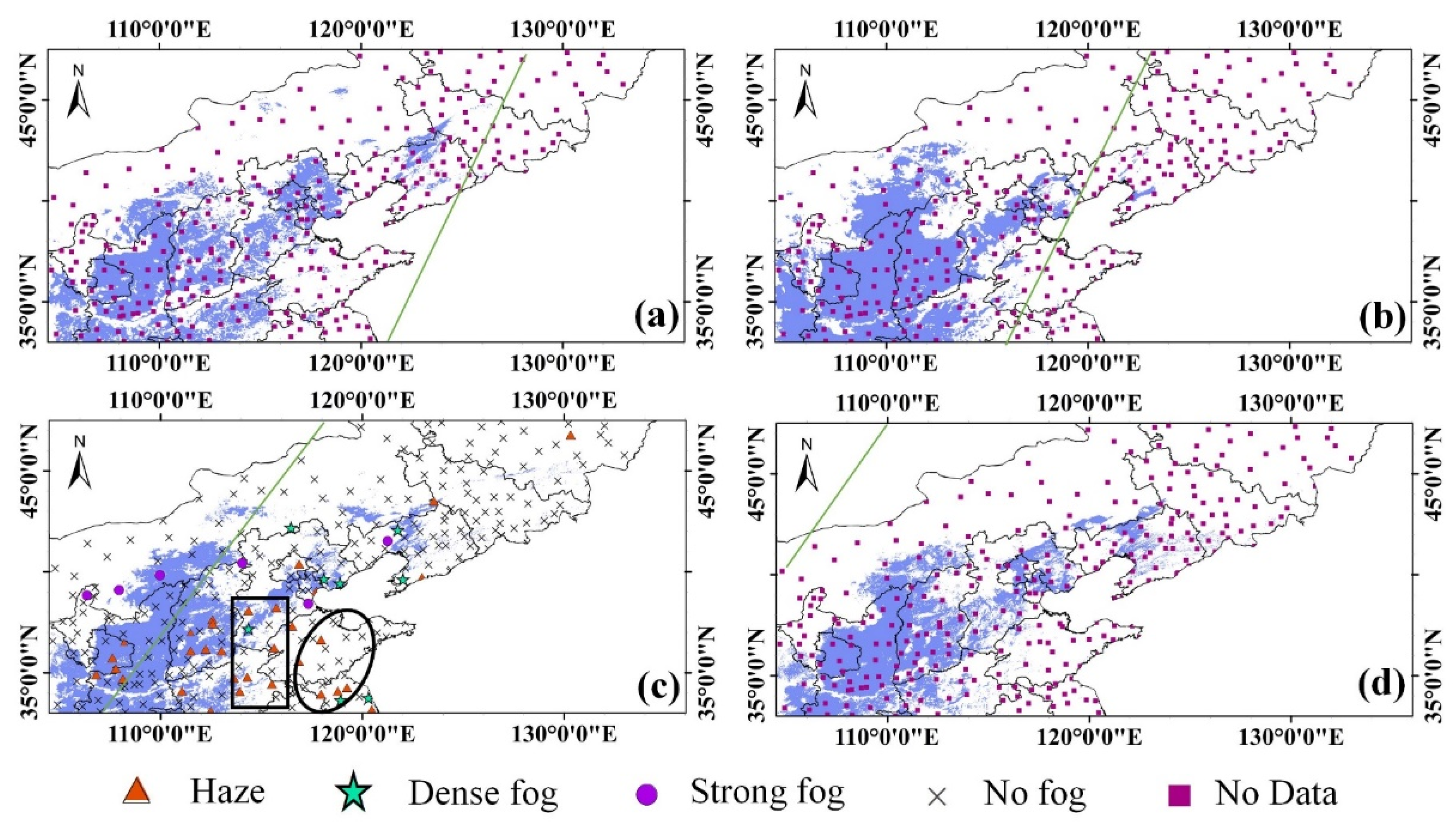
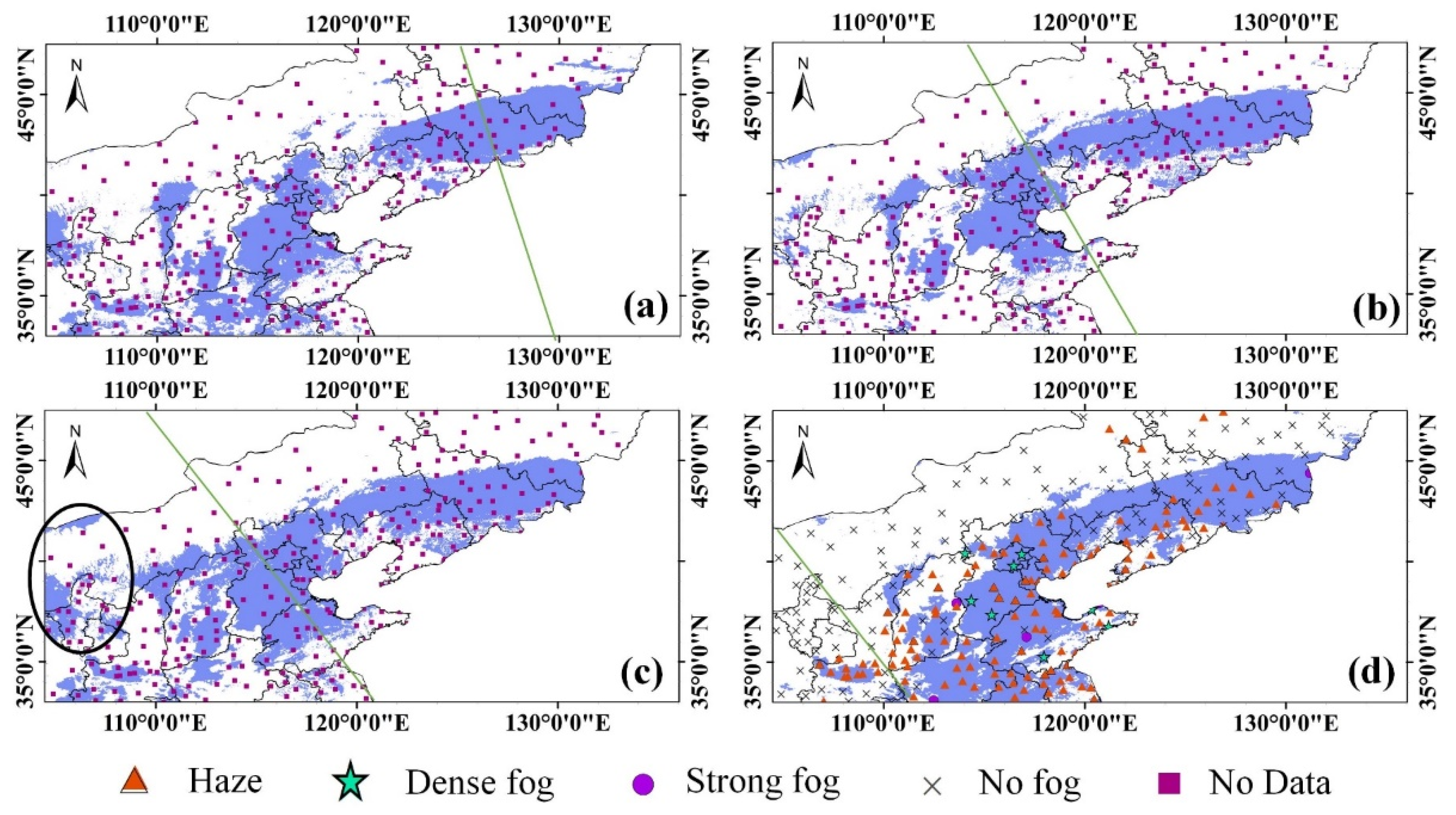
The fog is detected at dawn (7:00–8:30) and dusk (15:30–17:00) on 18 November 2016 over northern China (Figure 6 and Figure 7) through our algorithm, and ground observation sites at 8:00 or 17:00 are shown in Figure 6c and Figure 7d. The detection results show that the fog area increases from 7:00 to 7:30 and gradually decreases from 7:30–8:30. Comparing the position of the terminator line, it can be seen that the fog gradually dissipated after sunrise. With the aid of our algorithm, large areas of fog are detected in the central and western parts of the study area. Furthermore, the detection results of satellite data can capture the generation and disappearance of fog, which is highly consistent with the ground observations. Figure 6a shows that the fog was in the formation stage. The fog area was fragmented because it was interspersed with low cloud, resulting in incomplete fog detection results. Figure 6b shows that a relatively stable fog zone has formed, with fog covering the largest region before sunrise. As the terminator line continues to move westwards, the surface temperature in the eastern portion of the figure increases rapidly due to solar radiation, which causes fog to dissipate gradually (Figure 6c,d). The ground observation data show a high spatial consistence with the results of satellite fog detection (Figure 6c). The rectangular box in Figure 6c is located in the Chinese topographic transition zone according to the terrain of the study area (Figure 1), whose foggy area’s boundary is defined well because of the application of terrain data. The missing detection is primarily located in the eastern portion of the figure (circular box in Figure 6c). The main reason for this missing detection might originate from the influence of low clouds. Influenced by the characteristics of the passive sensor images, it is relatively difficult to detect the under-cloud fog for the algorithm.
Figure 7 shows the fog detection results at dusk from 15:30 to 17:00. The ground observation data show large areas of haze at 17:00. It also shows a high spatial consistence with the results of satellite fog detection (Figure 7d), which supports the performance of our fog detection approach (Figure 7d). Satellite detection results show that the area of fog takes on a relatively stable trend from 15:30 to 17:00 (Figure 7a–d). The false detection occurred to the left of the terminator line at 16:30 (circular box in Figure 7c), which is characterized by high topographic undulations and low cloud coverage. Overall, our algorithm successfully detected more than 80% of fog in the study area.
We validate the algorithm with the aid of 10 fog cases randomly selected from 18th November in 2016 to 3 January in 2017. The statistical evaluation shows that the overall POD, FAR and CSI of the algorithm are 84.0%, 16.4% and 72.0% at dawn (Table 2), respectively. The highest FAR and lowest CSI occurred on January 3, 2017. The main reason is attributed to the low clouds in the Inner Mongolia autonomous region and Northeast Plain, which are difficult to be isolated by infrared remote sensing at nighttime. Table 3 shows the accuracy at dusk, with the mean POD, FAR and CSI values are 83.7%, 15.8% and 72.6%, respectively. Overall, our algorithm demonstrates the broad potential of using deep learning for fog detection at dawn and dusk. We sum all the fog categories to validate the algorithm. It is very useful to evaluate the accuracies under different fog types. However, the observation points are insufficient to be divided into so many sub-datasets. Therefore, a small disturbance of the ground samples would generate great uncertainty on the validation. We will continue the collection of ground observation to validation the performance of our algorithm in our future research.
To evaluate the seasonal adaptability of the algorithm, eight dawn fog cases and five dusk fog cases were randomly selected from February to October 2017 (few fogs occur at dusk from April to July). Ground observations in 08:00 (February to March) and 05:00 (May to September) are adopted for the evaluation at dawn and dusk. Results are shown in Table 4 and Table 5. Overall, the POD, FAR and CSI are 66.8%, 45.1% and 43.6% at dawn, and 68.0%, 32.3% and 49.8% at dusk, which show the acceptable accuracy over different seasons. On the other hand, the detection accuracy in summer and autumn was significantly influenced by cloudiness. In summer, the algorithm’s performance is robust due to the apparent spectral and textural difference of the surface and fog/cloud. However, low clouds (liquid water clouds) in summer are more likely to be misclassified as fog. The FAR also increased due to the frequent cloud covering in autumn.
4. Discussion
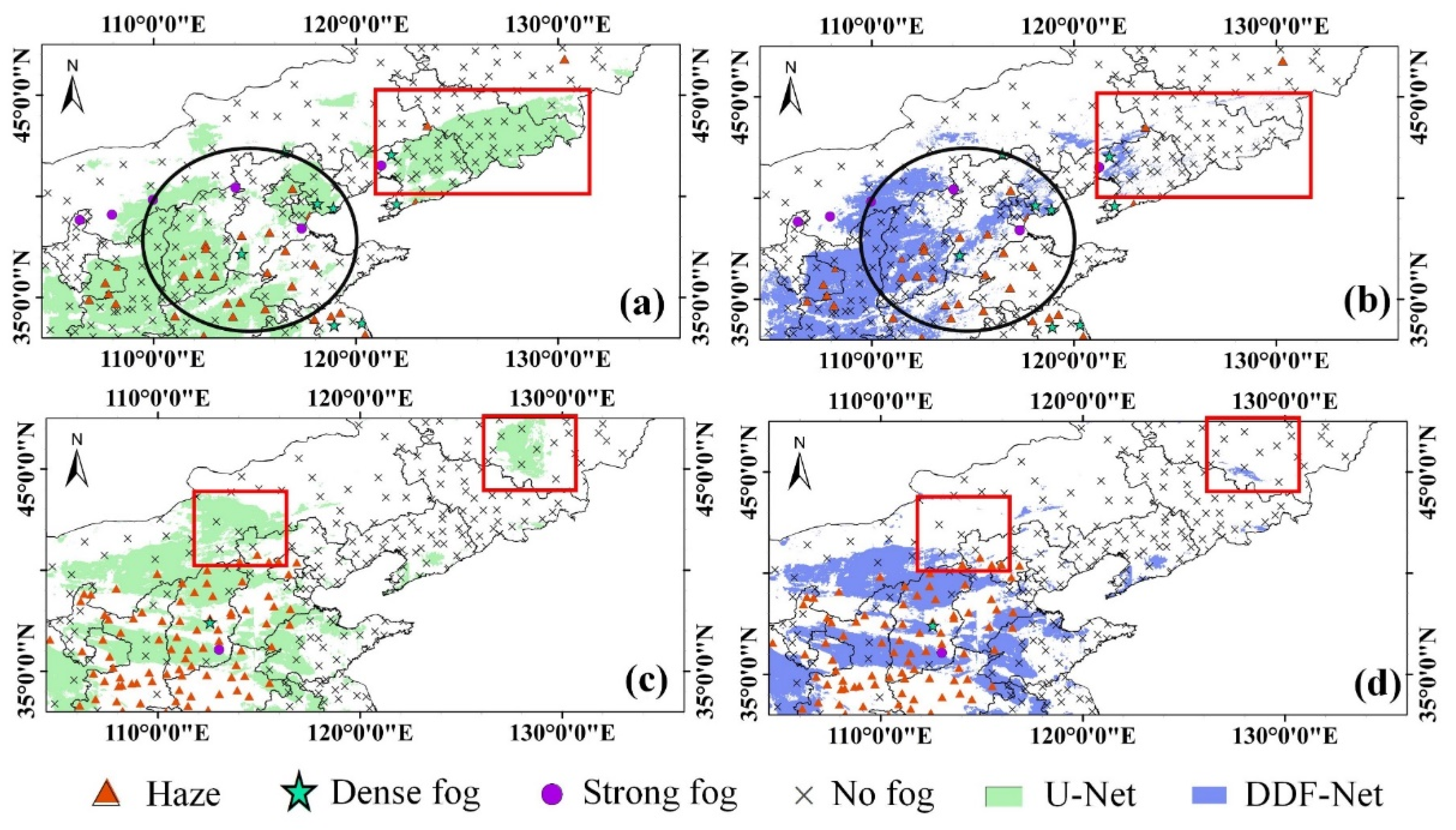
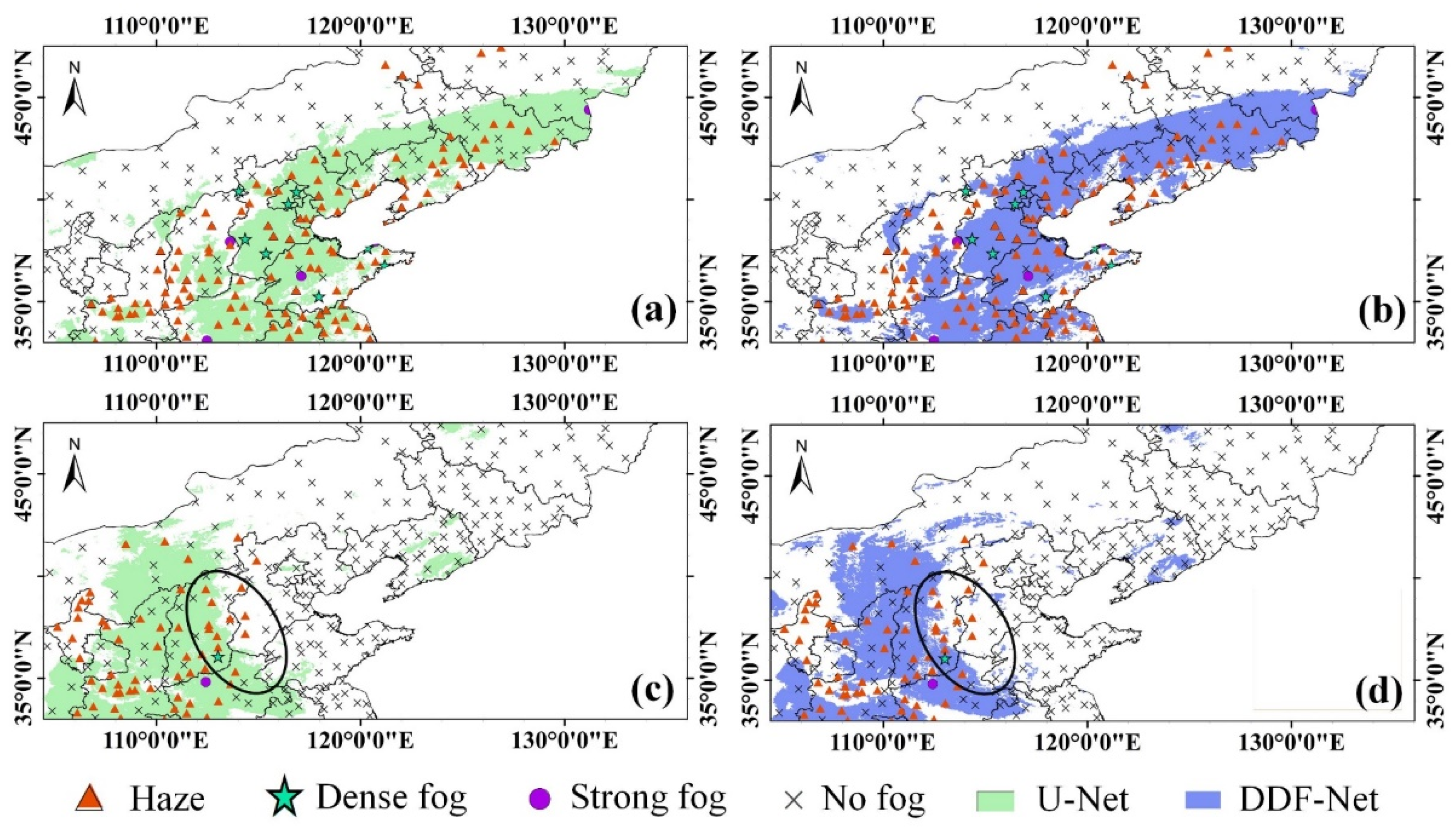
We further compare the performances of our algorithm with those of the previous studies. Specifically, fog detection results from the U-Net and DDF-Net are compared at 08:00 on 18 in November and 12 December in 2016, and at 17:00 on 18 November and 11 December in 2016. The comparisons are shown in Figure 8 and Figure 9. The ground observation indicates that fog area exceeding 85% has been successfully detected in the study area (Figure 8c,d and Figure 9a,b). Specifically, both algorithms detected fog more accurately at dawn (Figure 8c,d), and haze is detected more accurately by both algorithms at dusk (Figure 9a,b). On the other hand, both algorithms have missed detections due to medium and low cloud contamination (circular box in Figure 8a,b and Figure 9c,d). The false detection occurred at 8:00 (rectangular box in Figure 8c,d), which are mainly due to the interference of the low liquid water cloud. Compared with the U-Net, the DDF-Net shows more accurate detection accuracy. For example, the circular box in Figure 8a,b shows that fog edges of the U-Net are slightly coarse with a small proportion of low stratus being misclassified as fog, but the edge detection results of DDF-Net are more refined and the boundary of the foggy area is clearer. Secondly, U-Net detects low cloud as fog mistakenly in the daytime area with high SZA (rectangular box in Figure 8a,c), while the misclassified medium/high clouds are smaller in the DDF-Net (rectangular box in Figure 8b,d).
5. Conclusions
In this study, we developed a novel algorithm for fog detection at dawn and dusk, which is based on the U-Net model and incorporates a channel attention mechanism under-restriction. Several conclusions could be drawn after the execution and validation of the algorithm:
- (1)
- The DDF-Net could detect large-scale fog and has a more refined identification of the edge of the fog area. Both the DDF-Net and U-net are challenged in detecting fog during the periods of time when the fog is dissipating and when there are clouds, while the FAR of DDF-Net is lower than the latter.
- (2)
- The fog near the terminator line can be effectively separated from the surface, which is effective for identifying fog from the surface at dawn and dusk. Specially, the DDF-Net can effectively improve the misdetection of medium/low clouds near and far from the terminator line. The fog detection results are relatively stable with fewer false detections.
- (3)
- The algorithm is simple and efficient, with little human intervention. As a result, the fog detection results can be obtained in near real time and are well suited to the requirements for real-time detection of dawn and dusk fog over large areas of land.
Overall, this study provides a new deep learning-based approach for fog detection at dawn and dusk. Our algorithm shows great advantages and potential for overcoming the limitations of minor spectral differences for fog detection at dawn and dusk, which would significantly improve the satellite application in climate forecast. The limitation refers to the low performance of fog formation and dissipation in mountainous areas with highly complex terrain. Two issues would be addressed in our future research. Firstly, other geographical parameters (i.e., latitude and surface temperature, etc.) would also affect the fog formation, which should be addressed in the algorithm to improve the accuracy of satellite fog detection. Secondly, a public fog dataset for each season would be developed and published for supporting the management of traffic and public health.
Author Contributions
Conceptualization, Y.R.; methodology, Y.R. and H.F.; software, Y.R.; validation, Y.R., H.M. and Z.L.; formal analysis, Y.R.; investigation, X.W. and Y.L.; resources, X.W.; data curation, X.W.; writing—original draft preparation, Y.R.; writing—review and editing, H.F. and H.M.; visualization, Y.R. and Z.L.; supervision, H.M. and H.F.; project administration, H.M.; funding acquisition, H.M. and H.F. All authors have read and agreed to the published version of the manuscript.
Funding
This research was funded by the National Natural Science Foundation of China, grant number 42071334 and 42071378.
Data Availability Statement
The Himawari-8 data supporting the findings of this study are openly available at https://www.eorc.jaxa.jp/ptree/ (accessed on 17 April 2020). The ground observation data can be archived at the following website https://data.cma.cn/ (accessed on 20 April 2020). The SRTM1-DEM data can be archived at the following website https://www.usgs.gov/ (accessed on 5 May 2020).
Acknowledgments
The authors are grateful to JMA for making the Himawari-8 data available. We are also grateful to the National Satellite Meteorological Center for providing access to the Meteorological station visibility data of our research.
Conflicts of Interest
The authors declare no conflict of interest.
References
- World Meteorological Organization (WMO). International Meteorological Vocabulary; Secretariat of the WMO: Geneva, Switzerland, 1992; p. 782. [Google Scholar]
- Ma, H.; Li, Y.; Wu, X.; Feng, H.; Ran, Y.; Jiang, B.; Wang, W. A large-region fog detection algorithm at dawn and dusk for high-frequency Himawari-8 satellite data. Int. J. Remote Sens. 2022, 43, 2620–2637. [Google Scholar] [CrossRef]
- Nilo, S.T.; Romano, F.; Cermak, J.; Cimini, D.; Ricciardelli, E.; Cersosimo, A.; Di Paola, F.; Gallucci, D.; Gentile, S.; Geraldi, E. Fog detection based on meteosat second generation-spinning enhanced visible and infrared imager high resolution visible channel. Remote Sens. 2018, 10, 541. [Google Scholar] [CrossRef]
- Kang, L.; Miao, Y.Y.; Miao, M.S.; Hu, Z.Y. The Harm of Fog and Thick Haze to the Body and the Prevention of Chinese Medicine. In Proceedings of the 2nd International Conference on Biomedical and Biological Engineering 2017 (BBE 2017), Guilin, China, 26–28 May 2017; Atlantis Press: Amsterdam, The Netherlands, 2017; pp. 119–124. [Google Scholar] [CrossRef]
- Yoo, J.M.; Choo, G.H.; Lee, K.H.; Wu, D.L.; Yang, J.H.; Park, J.D.; Choi, Y.S.; Shin, D.B.; Jeong, J.H.; Yoo, J.M. Improved detection of low stratus and fog at dawn from dual geostationary (COMS and FY-2D) satellites. Remote Sens. Environ. 2018, 211, 292–306. [Google Scholar] [CrossRef]
- Lee, J.R.; Chung, C.Y.; Ou, M.L. Fog detection using geostationary satellite data: Temporally continuous algorithm. Asia-Pac. J. Atmos. Sci. 2011, 47, 113–122. [Google Scholar] [CrossRef]
- Hunt, G.E. Radiative properties of terrestrial clouds at visible and infra-red thermal window wavelengths. Q. J. R. Meteorol. Soc. 1973, 99, 346–369. [Google Scholar] [CrossRef]
- Eyre, J. Detection of fog at night using Advanced Very High Resolution Radiometer (AVHRR) imagery. Meteorol. Mag. 1984, 113, 266–271. [Google Scholar]
- Turner, J.; Allam, R.; Maine, D. A case-study of the detection of fog at night using channels 3 and 4 on the Advanced Very High-Resolution Radiometer (AVHRR). Meteorol. Mag. 1986, 115, 285–290. [Google Scholar]
- Bendix, J. Fog climatology of the Po Valley. Riv. Meteorol. Aeronaut. 1994, 54, 25–36. [Google Scholar]
- Bendix, J. A case study on the determination of fog optical depth and liquid water path using AVHRR data and relations to fog liquid water content and horizontal visibility. Int. J. Remote Sens. 1995, 16, 515–530. [Google Scholar] [CrossRef]
- Cermak, J.; Bendix, J. Dynamical Nighttime Fog/Low Stratus Detection Based on Meteosat SEVIRI Data: A Feasibility Study. Pure Appl. Geophys. 2007, 164, 1179–1192. [Google Scholar] [CrossRef]
- Cermak, J.; Bendix, J. A novel approach to fog/low stratus detection using Meteosat 8 data. Atmos. Res. 2008, 87, 279–292. [Google Scholar] [CrossRef]
- Chaurasia, S.; Sathiyamoorthy, V.; Paul Shukla, B.; Simon, B.; Joshi, P.C.; Pal, P.K. Night time fog detection using MODIS data over Northern India. Met Apps. 2011, 18, 483–494. [Google Scholar] [CrossRef]
- Weston, M.; Temimi, M. Application of a Nighttime Fog Detection Method Using SEVIRI Over an Arid Environment. Remote Sens. 2020, 12, 2281. [Google Scholar] [CrossRef]
- Gurka, J.J. The Role of Inward Mixing in the Dissipation of Fog and Stratus. Mon. Weather Rev. 1978, 106, 1633–1635. [Google Scholar] [CrossRef]
- Rao, P.K.; Holmes, S.J.; Anderson, R.K.; Winston, J.S.; Lehr, P.E. Weather Satellites: Systems, Data, and Environmental Applications; American Meteorological Society: Boston, MA, USA, 1990; p. 516. [Google Scholar]
- Chaurasia, S.; Gohil, B.S. Detection of Day Time Fog Over India Using INSAT-3D Data. IEEE J. Sel. Top. Appl. Earth Obs. Remote Sens. 2015, 8, 4524–4530. [Google Scholar] [CrossRef]
- Drönner, J.; Egli, S.; Thies, B.; Bendix, J.; Seeger, B. FFLSD—Fast Fog and Low Stratus Detection tool for large satellite time-series. Comput. Geosci. 2019, 128, 51–59. [Google Scholar] [CrossRef]
- Yang, J.H.; Yoo, J.M.; Choi, Y.S. Advanced Dual-Satellite Method for Detection of Low Stratus and Fog near Japan at Dawn from FY-4A and Himawari-8. Remote Sens. 2021, 13, 1042. [Google Scholar] [CrossRef]
- Hůnová, I.; Brabec, M.; Malý, M.; Dumitrescu, A.; Geletič, J. Terrain and its effects on fog occurrence. Sci. Total Environ. 2021, 768, 144359. [Google Scholar] [CrossRef]
- Shang, H.; Chen, L.; Letu, H.; Zhao, M.; Li, S.; Bao, S. Development of a daytime cloud and haze detection algorithm for Himawari-8 satellite measurements over central and eastern China. J. Geophys. Res. Atmos. 2017, 122, 3528–3543. [Google Scholar] [CrossRef]
- LeCun, Y.; Bengio, Y.; Hinton, G. Deep learning. Nature 2015, 521, 436–444. [Google Scholar] [CrossRef]
- Jeppesen, J.H.; Jacobsen, R.H.; Inceoglu, F.; Toftegaard, T.S. A cloud detection algorithm for satellite imagery based on deep learning. Remote Sens. Environ. 2019, 229, 247–259. [Google Scholar] [CrossRef]
- Wu, X.; Shi, Z.; Zou, Z. A geographic information-driven method and a new large scale dataset for remote sensing cloud/snow detection. Isprs. J. Photogramm. 2021, 174, 87–104. [Google Scholar] [CrossRef]
- Hu, J.; Shen, L.; Sun, G. Squeeze-and-excitation networks. In Proceedings of the IEEE Conference on Computer Vision and Pattern recognition, Salt Lake City, UT, USA, 18–23 June 2018; pp. 7132–7141. [Google Scholar] [CrossRef]
- Kingma, D.P.; Ba, J. Adam: A method for stochastic optimization. arXiv 2014, arXiv:1412.6980. [Google Scholar] [CrossRef]
- Ding, Y.; Liu, Y. Analysis of long-term variations of fog and haze in China in recent 50 years and their relations with atmospheric humidity. Sci. China Earth Sci. 2014, 57, 36–46. [Google Scholar] [CrossRef]
- Chen, H.; Wang, H. Haze Days in North China and the associated atmospheric circulations based on daily visibility data from 1960 to 2012. J. Geophys. Res. Atmos. 2015, 120, 5895–5909. [Google Scholar] [CrossRef]
- Bessho, K.; Date, K.; Hayashi, M.; Ikeda, A.; Imai, T.; Inoue, H.; Kumagai, Y.; Miyakawa, T.; Murata, H.; Ohno, T. An introduction to Himawari-8/9—Japan’s new-generation geostationary meteorological satellites. J. Meteorol. Soc. Jpn. 2016, 94, 151–183. [Google Scholar] [CrossRef]
- Ishida, H.; Nakajima, T.Y. Development of an unbiased cloud detection algorithm for a spaceborne multispectral imager. J. Geophys. Res. 2009, 114. [Google Scholar] [CrossRef]
- Knudby, A.; Latifovic, R.; Pouliot, D. A cloud detection algorithm for AATSR data, optimized for daytime observations in Canada. Remote Sens. Environ. 2011, 115, 3153–3164. [Google Scholar] [CrossRef]
- Cermak, J.; Bendix, J. Detecting ground fog from space—A microphysics-based approach. Int. J. Remote Sens. 2011, 32, 3345–3371. [Google Scholar] [CrossRef]
- GB/T 27964-2011GB/T; Grade of Fog Forecast. China Meteorological Administration (CMA): Beijing, China, 2011. (In Chinese)
- Zeiler, M.; Fergus, R. Visualizing and understanding convolutional networks. In Proceedings of the European Conference on Computer Vision, Zurich, Switzerland, 6–12 September 2014; pp. 818–833. [Google Scholar]
- Rumelhart, D.E.; Hinton, G.E.; Williams, R.J. Learning representations by back-propagating errors. Nature 1986, 323, 533–536. [Google Scholar] [CrossRef]
- Ronneberger, O.; Fischer, P.; Brox, T. U-Net: Convolutional Networks for Biomedical Image Segmentation. In Proceedings of the Medical Image Computing and Computer-Assisted Intervention—MICCAI 2015, Munich, Germany, 5–9 October 2015; Springer International Publishing: Cham, Switzerland, 2015; pp. 234–241. [Google Scholar]
- Shao, Z.; Pan, Y.; Diao, C.; Cai, J. Cloud Detection in Remote Sensing Images Based on Multiscale Features-Convolutional Neural Network. IEEE Trans. Geosci. Remote 2019, 57, 4062–4076. [Google Scholar] [CrossRef]
- Mohajerani, S.; Krammer, T.A.; Saeedi, P. Cloud detection algorithm for remote sensing images using fully convolutional neural networks. arXiv 2018, arXiv:1810.05782. [Google Scholar] [CrossRef] [Green Version]
- Ioffe, S.; Szegedy, C. Batch Normalization: Accelerating Deep Network Training by Reducing Internal Covariate Shift. In Proceedings of the 32nd International Conference on Machine Learning, Lille, France, 6–11 July 2015; Francis, B., David, B., Eds.; PMLR: San Diego, CA, USA, 2015; pp. 448–456. [Google Scholar]
Figure 1.
The study area.

Figure 2.
The Schematic diagram of the deep learning model. Relu is used to achieve non-linear transformation between the CL and PL layers.
Figure 2.
The Schematic diagram of the deep learning model. Relu is used to achieve non-linear transformation between the CL and PL layers.

Figure 3.
Flow chart of the methodology.

Figure 4.
The DDF-Net’s architecture. The top/bottom numbers of the rectangle represent the channels of the feature map, and the right numbers are the size of the feature map.
Figure 4.
The DDF-Net’s architecture. The top/bottom numbers of the rectangle represent the channels of the feature map, and the right numbers are the size of the feature map.

Figure 5.
The process of making the H8/AHI-DEM-Fm dataset.

Figure 6.
The fog detection results at (a) 7:00, (b) 7:30, (c) 8:00 and (d) 8:30 on 18 November 2016. The triangle, star, circle, and cross symbols represent haze, dense fog, strong fog, and non-fog stations, respectively. The square symbol indicates that there is no observation data because of the limit monitoring frequency. The blue area is the fog detected by our algorithm. All the times are at the Beijing Time (8 h later than the Universal Time Coordinated (UTC)) and the green line is the terminator line.

Figure 7.
The fog detection results at (a) 15:30, (b) 16:00, (c) 16:30 and (d) 17:00 on 18 November 2016. The triangle, star, circle, and cross symbols represent haze, dense fog, strong fog, and non-fog stations, respectively. The square symbol indicates that there is no observation data because of the limit monitoring frequency. The blue area is the fog detected by our algorithm. All the times are at the Beijing Time (8 h later than the Universal Time Coordinated (UTC)) and the green line is the terminator line.

Figure 8.
The fog detection results of U-Net and DDF-Net at 08:00 (18 November 2016 (a,b) and 12 December 2016 (c,d)). The triangle, star, circle, and cross symbols represent haze, dense fog, strong fog, and non-fog stations, respectively. The green area is the fog detected by U-Net. The blue area is the fog detected by DDF-Net. All the times are at the Beijing Time (8 h later than the Universal Time Coordinated (UTC)).

Figure 9.
The fog detection results of U-Net and DDF-Net at 17:00 (18 November 2016 (a,b) and 11 December 2016 (c,d)). The triangle, star, circle, and cross symbols represent haze, dense fog, strong fog, and non-fog stations, respectively. The green area is the fog detected by U-Net. The blue area is the fog detected by DDF-Net. All the times are at the Beijing Time (8 h later than the Universal Time Coordinated (UTC)).


Table 1.
Training platform and parameter configuration information.
| Parameter Configuration | Platform and Version |
|---|---|
| GPU | NVIDIA GeForce RTX 2080Ti (NVIDIA Corporation, Santa Clara, CA, United States) |
| Memory | 11GB |
| Operating system | Windows 10 |
| Programming language | Python3.6.6 |
| Framework | PyTorch1.5.1 |
| Cuda | 10.0 |
| Batch size | 8 |
| Epoch | 1500 |
| Decaying Epoch | 1440 |
| 0.0035 |
Table 2.
Fog detection accuracy at 08:00 (BT).
| Date | Satellite Detection | Ground Observation (Fog) | Ground Observation (Nonfog) | POD | FAR | CSI |
|---|---|---|---|---|---|---|
| 18 November 2016 | Fog Nonfog | 34 12 | 7 210 | 0.739 | 0.171 | 0.642 |
| 12 December 2016 | Fog Nonfog | 44 3 | 6 255 | 0.936 | 0.120 | 0.830 |
| 18 December 2016 | Fog Nonfog | 16 3 | 3 276 | 0.842 | 0.158 | 0.727 |
| 20 December 2016 | Fog Nonfog | 19 4 | 2 322 | 0.826 | 0.095 | 0.760 |
| 3 January 2017 | Fog Nonfog | 18 3 | 7 381 | 0.857 | 0.280 | 0.643 |
| mean | 0.840 | 0.164 | 0.720 | |||
Table 3.
Fog detection accuracy at 17:00 (BT).
| Date | Satellite Detection | Ground Observation (Fog) | Ground Observation (Nonfog) | POD | FAR | CSI |
|---|---|---|---|---|---|---|
| 17 November 2016 | Fog Nonfog | 11 2 | 2 209 | 0.846 | 0.154 | 0.733 |
| 18 November 2016 | Fog Nonfog | 42 3 | 3 238 | 0.933 | 0.067 | 0.875 |
| 11 December 2016 | Fog Nonfog | 44 8 | 10 372 | 0.846 | 0.185 | 0.710 |
| 18 December 2016 | Fog Nonfog | 12 3 | 4 277 | 0.800 | 0.250 | 0.632 |
| 28 December 2016 | Fog Nonfog | 19 6 | 3 307 | 0.760 | 0.136 | 0.679 |
| mean | 0.837 | 0.158 | 0.726 | |||
Table 4.
Fog detection accuracy at dawn over different seasons.
| Ground Observation Time | Cases | Satellite Detection | Ground Observation (Fog) | Ground Observation (Nonfog) | POD | FAR | CSI |
|---|---|---|---|---|---|---|---|
| 8:00 | 5 February 2017, 8:00 | Fog Nonfog | 21 3 | 9 402 | 0.875 | 0.300 | 0.636 |
| 8:00 | 17 March 2017, 7:00 | Fog Nonfog | 5 2 | 4 413 | 0.714 | 0.444 | 0.455 |
| 5:00 | 5 May 2017, 6:00 | Fog Nonfog | 8 5 | 15 409 | 0.615 | 0.652 | 0.286 |
| 5:00 | 27 June 2017, 6:00 | Fog Nonfog | 24 11 | 13 392 | 0.686 | 0.351 | 0.500 |
| 5:00 | 29 July 2017, 6:00 | Fog Nonfog | 6 5 | 13 426 | 0.545 | 0.684 | 0.250 |
| 5:00 | 31 August 2017, 5:00 | Fog Nonfog | 12 9 | 14 399 | 0.571 | 0.538 | 0.343 |
| 5:00 | 17 September 2017, 5:00 | Fog Nonfog | 5 3 | 3 377 | 0.625 | 0.375 | 0.455 |
| 5:00 | 12 October 2017, 6:00 | Fog Nonfog | 22 9 | 8 415 | 0.710 | 0.267 | 0.564 |
| mean | 0.668 | 0.451 | 0.436 | ||||
Table 5.
Fog detection accuracy at dusk over different seasons.
| Ground Observation Time | Cases | Satellite Detection | Ground Observation (Fog) | Ground Observation (Nonfog) | POD | FAR | CSI |
|---|---|---|---|---|---|---|---|
| 17:00 | 21 February 2017, 17:00 | Fog Nonfog | 12 14 | 3 395 | 0.462 | 0.200 | 0.414 |
| 17:00 | 13 March 2017, 17:00 | Fog Nonfog | 24 7 | 11 417 | 0.774 | 0.314 | 0.571 |
| 20:00 | 22 August 2017, 19:00 | Fog Nonfog | 0 7 | 0 487 | -- | -- | -- |
| 17:00 | 15 September 2017, 18:00 | Fog Nonfog | 19 8 | 12 377 | 0.704 | 0.387 | 0.487 |
| 17:00 | 5 October 2017, 18:00 | Fog Nonfog | 14 4 | 9 437 | 0.778 | 0.391 | 0.519 |
| mean | 0.680 | 0.323 | 0.498 | ||||
Publisher’s Note: MDPI stays neutral with regard to jurisdictional claims in published maps and institutional affiliations. |
© 2022 by the authors. Licensee MDPI, Basel, Switzerland. This article is an open access article distributed under the terms and conditions of the Creative Commons Attribution (CC BY) license (https://creativecommons.org/licenses/by/4.0/).
Share and Cite
MDPI and ACS Style
Ran, Y.; Ma, H.; Liu, Z.; Wu, X.; Li, Y.; Feng, H. Satellite Fog Detection at Dawn and Dusk Based on the Deep Learning Algorithm under Terrain-Restriction. Remote Sens. 2022, 14, 4328. https://doi.org/10.3390/rs14174328
AMA Style
Ran Y, Ma H, Liu Z, Wu X, Li Y, Feng H. Satellite Fog Detection at Dawn and Dusk Based on the Deep Learning Algorithm under Terrain-Restriction. Remote Sensing. 2022; 14(17):4328. https://doi.org/10.3390/rs14174328
Chicago/Turabian StyleRan, Yinze, Huiyun Ma, Zengwei Liu, Xiaojing Wu, Yanan Li, and Huihui Feng. 2022. "Satellite Fog Detection at Dawn and Dusk Based on the Deep Learning Algorithm under Terrain-Restriction" Remote Sensing 14, no. 17: 4328. https://doi.org/10.3390/rs14174328
Note that from the first issue of 2016, this journal uses article numbers instead of page numbers. See further details here.