
Deep Pansharpening via 3D Spectral Super-Resolution Network and Discrepancy-Based Gradient Transfer

1
Shaanxi Key Laboratory for Network Computing and Security Technology, Department of Computer Science and Engineering, Xi’an University of Technology, No. 5 South Jinhua Road, Xi’an 710048, China
2
Xi’an Institute of Optics and Precision Mechanics, Chinese Academy of Sciences, Xi’an 710119, China
3
Key Laboratory of Space Precision Measurement Technology, Chinese Academy of Sciences, Xi’an 710119, China
*
Author to whom correspondence should be addressed.
Remote Sens. 2022, 14(17), 4250; https://doi.org/10.3390/rs14174250
Submission received: 21 July 2022
/
Revised: 10 August 2022
/
Accepted: 23 August 2022
/
Published: 29 August 2022
(This article belongs to the Section Remote Sensing Image Processing)
Abstract
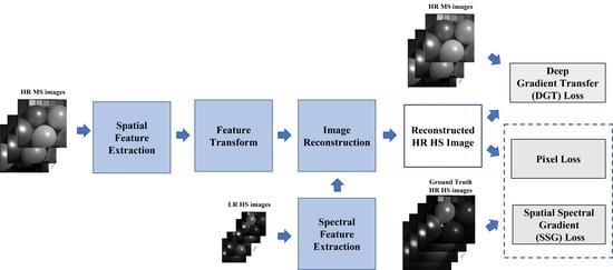
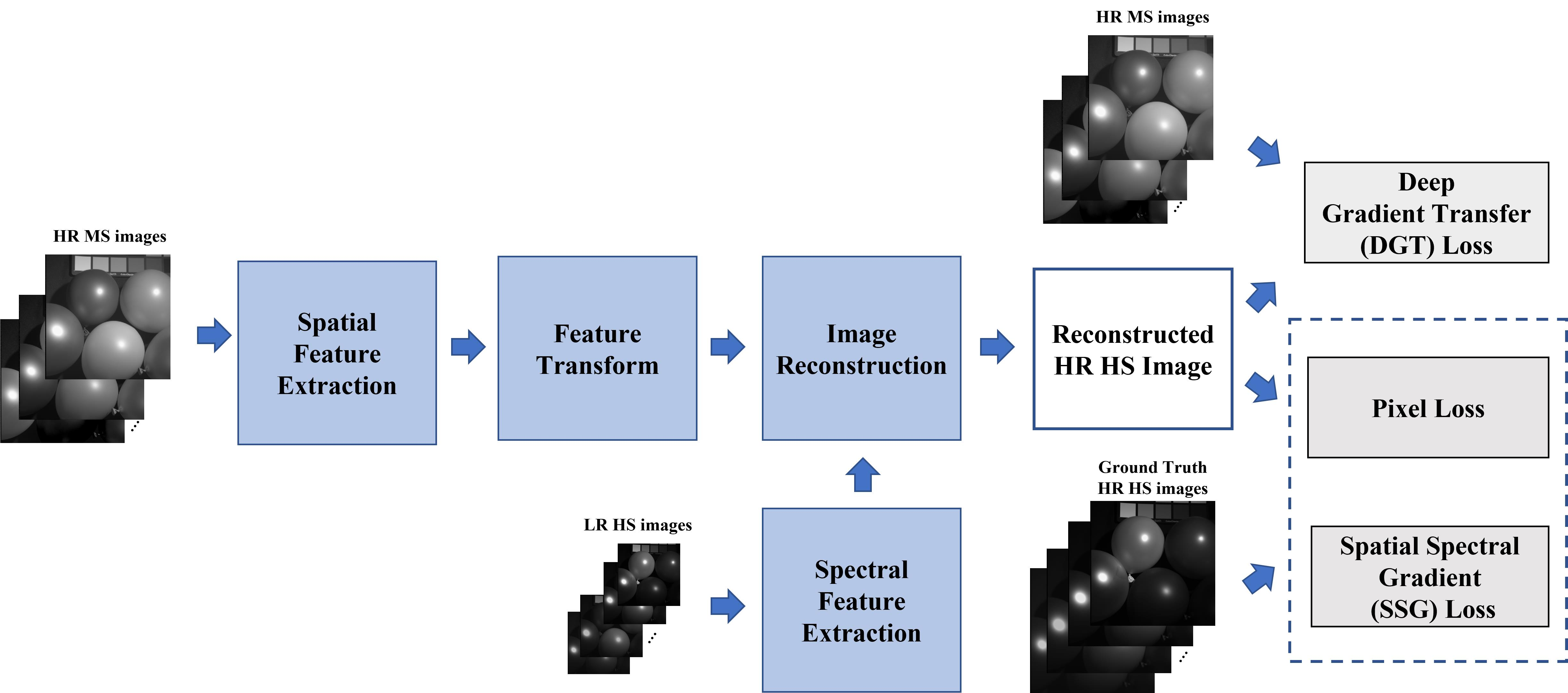
:High-resolution (HR) multispectral (MS) images contain sharper detail and structure compared to the ground truth high-resolution hyperspectral (HS) images. In this paper, we propose a novel supervised learning method, which considers pansharpening as the spectral super-resolution of high-resolution multispectral images and generates high-resolution hyperspectral images. The proposed method learns the spectral mapping between high-resolution multispectral images and the ground truth high-resolution hyperspectral images. To consider the spectral correlation between bands, we build a three-dimensional (3D) convolution neural network (CNN). The network consists of three parts using an encoder–decoder framework: spatial/spectral feature extraction from high-resolution multispectral images/low-resolution (LR) hyperspectral images, feature transform, and image reconstruction to generate the results. In the image reconstruction network, we design the spatial–spectral fusion (SSF) blocks to reuse the extracted spatial and spectral features in the reconstructed feature layer. Then, we develop the discrepancy-based deep hybrid gradient (DDHG) losses with the spatial–spectral gradient (SSG) loss and deep gradient transfer (DGT) loss. The spatial–spectral gradient loss and deep gradient transfer loss are developed to preserve the spatial and spectral gradients from the ground truth high-resolution hyperspectral images and high-resolution multispectral images. To overcome the spectral and spatial discrepancy between two images, we design a spectral downsampling (SD) network and a gradient consistency estimation (GCE) network for hybrid gradient losses. In the experiments, it is seen that the proposed method outperforms the state-of-the-art methods in the subjective and objective experiments in terms of the structure and spectral preservation of high-resolution hyperspectral images.
1. Introduction
A hyperspectral (HS) image is a spatial–spectral data cube, which consists of spatial and spectral information. The large amount of spectral information in HS images improves the performance of target detection [1], denoising [2], and image classification [3,4] compared to multispectral (MS) images (such as RGB images). Thus, high-resolution (HR) HS images are required in a vast amount of remote sensing applications. However, capturing the HR HS images is still a challenging task because of technical limitations. One of the methods is the single-image super-resolution method, which generates the HR HS images from low-resolution (LR) HS images. Because of the technical developments, multi-sensor fusion has attracted more attention in recent years. MS images mainly focus on spatial resolution with a few bands, while HS images provide a large number of bands with low resolution. Thus, pansharpening (i.e., the fusion of HR MS images and LR HS images) emerges in the remote sensing area. Compared to single-image super-resolution, pansharpening provides more accurate HR HS images with auxiliary HR MS images.
2. Related Work
So far, traditional pansharpening methods can be mainly divided into four parts: component substitution (CS), multiresolution analysis (MRA), Bayesian methods, and variational methods. CS-based methods split the HS and MS images into spatial and spectral domains. The spatial information of MS images was utilized to enhance the spatial resolution of HS images [5]. Yang et al. proposed HS computational imaging using collaborative Tucker3 tensor decomposition [6]. The Tucker3 tensor decomposition was developed to model the low rankness and similarities of nonlocal patches. The spatial factor matrices and the core tensor of panchromatic images by Tucker3 tensor decomposition are utilized to constrain the spatial structure of HS images. MRA methods first employed multiscale filters to decompose the MS and HS images. They transferred the structures of MS images to HS images in each sub-band. Several decomposition methods were utilized such as high-pass filters, generalized Laplacian pyramids, and undecimated discrete wavelet transform [7,8,9]. Bayesian methods model a posterior probability of HR HS images and utilize Bayesian theory to predict the estimated HR images [10]. The variational approach was derived from Bayesian methods. Researchers introduced some suitable prior knowledge to probability terms and then transformed the Bayesian problem into an optimization problem, e.g., a dynamic sparsity regularizer [11] and multi-order gradient regularization [12].
In recent years, with the rise of the machine learning methods, some learning-based methods have been introduced to the pansharpening problem. Among them, more and more researchers employ deep learning to improve the performance of pansharpening. Masi et al. borrowed the idea from image super-resolution and built a three-layer convolutional network for pansharpening [13]. Shao et al. [14] considered the pansharpening problem as image fusion. They proposed two branch network architectures, which were used to extract the features from LR HS images and HR MS images, respectively. Then, two features were fused to generate the high-resolution HS results. Some researchers employed deep learning to learn the prior of HR HS images and then imported the learned prior into the optimization problem. Li et al. [15] proposed the detail-based deep Laplacian pansharpening method to improve the spatial resolution of HS images. The spatial and spectral details were learned by deep learning. Dian et al. utilized the residual learning to learn the image prior [16], and Xie et al. built the elaborated neural network to learn the high frequency of HR HS images [17]. Wang et al. integrated learned deep priors into the objective function derived from the degradation model [18]. The deep priors were learned using a two-stream fusion network. The regularization parameter was automatically selected using a golden section search strategy. Other researchers focused on the design of the loss function. Luo et al. [19] proposed an unsupervised convolutional neural network architecture with a set of specific design losses for spectral and spatial constraints between MS and HS images. Zhou et al. proposed the perceptual loss for an unsupervised pansharpening method [20]. The perceptual loss consisted of the pixel level loss, feature level loss, and GAN loss. Finally, some researchers considered pansharpening as the spectral super-resolution. Ozcelik et al. employed the colorization concept for HS pansharpening and proposed the panchromatic image colorization based on a generative adversarial network (GAN) [21]. However, they only considered one to three spectral channels’ mapping and utilized a 2D CNN without considering spectral correlations.
In this paper, we propose a deep HS pansharpening method based on the spectral super-resolution. The network is based on a 3D encoder–decoder framework, which consists of spatial/spectral feature extraction, feature transform, and image reconstruction. A 3D CNN is employed to consider the spectral correlation with thespectral super-resolution. Moreover, we propose the discrepancy-based deep hybrid gradient (DDHG) losses, which transfer the HR HS and HR MS image gradients considering the discrepancy. Finally, it is shown by experiments that the proposed method achieves the best performance in structure and spectral preservation from the HR HS images compared to the state-of-the-art methods. The main contributions of this paper are summarized as follows:
- We propose a supervised 3D-CNN-based spectral super-resolution network of HR MS images for pansharpening. The 3D CNN is employed to consider the spatial and spectral correlation simultaneously with thespectral super-resolution. Compared to the state-of-the-art methods, extensive experiments show that the proposed method achieves the best performance in spectral and spatial preservation from HR HS images.
- The 3D spectral super-resolution network constructs the encoder–decoder framework. In the decoder part, we design the image reconstruction network with a set of skip connections and spatial–spectral fusion (SSF) blocks, which fuse the spatial and spectral features efficiently.
- We define the discrepancy-based deep hybrid gradient (DDHG) losses, which contain the spatial–spectral gradient (SSG) loss and deep gradient transfer (DGT) losses. The losses are developed to constrain the spatial and spectral consistency from the ground truth HS images and HR MS images. To overcome the spatial and spectral discrepancy between two images, we design the spectral downsampling (SD) network and gradient consistency estimation (GCE) network in the DDHG losses.
3. Proposed Method
Given LR HS images and HR MS images , the objective of pansharpening problem is to generate the HR HS images . and are the width and height of LR HS images and HR MS images. The relationship of the width and height between HS and MS images is and , where s is the scale factor. L and l are the channels of the HS and MS images. Thus, the main target is to generate the resulting images with high spatial and spectral resolution. In this paper, we considered the pansharpening problem as the spectral super-resolution, which enhances the spectral channels of HR MS images. We built the 3D-CNN-based encoder–decoder neural network, which extracts the spatial and spectral features from the input HR MS and LR HS images and then reuses them in image reconstruction. The proposed method considers a more general case with arbitrary spectral channels’ enhancement and employs 3D CNN to take the spectral correlation into account. Moreover, we define the DDHG loss function to minimize the spatial and spectral distortion considering the spectral and spatial discrepancy.
3.1. Motivation
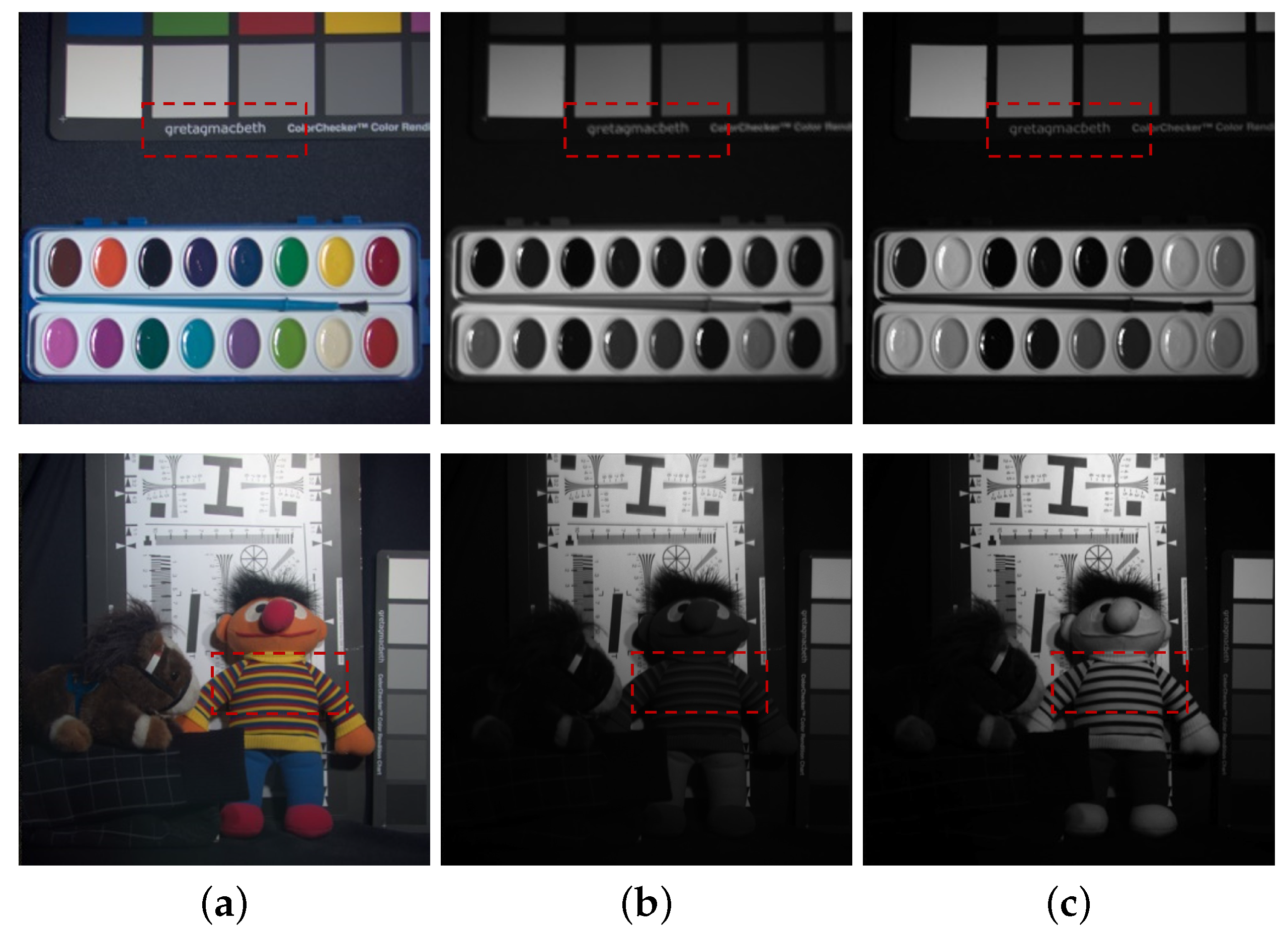
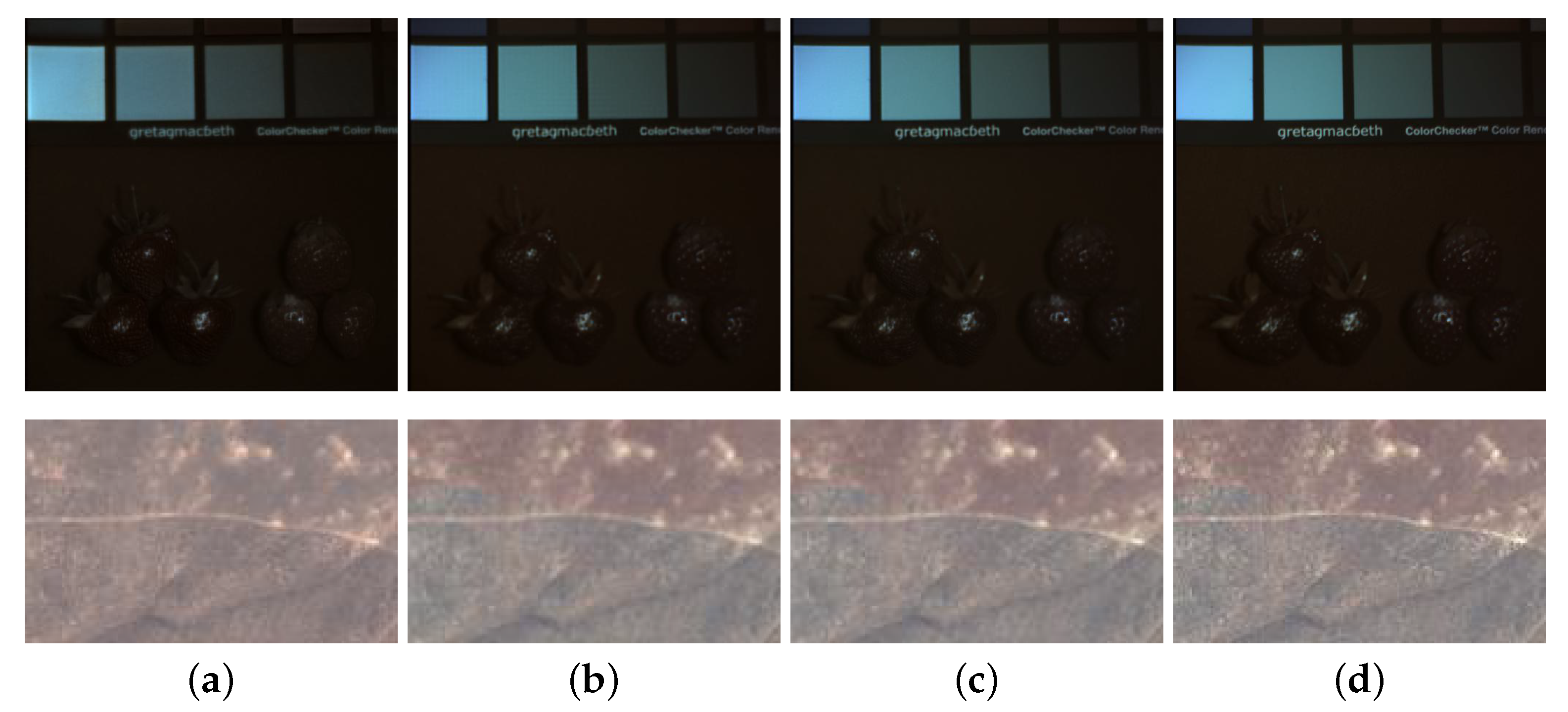
Figure 1 shows HR MS images and HR HS images at bands 3 and 27 for test image paints and chart and stuffed toy in the CAVE dataset [22]. It is shown that HR MS images provide a sharper structure and detail compared to the ground truth HS images (see the red blocks in the first row of Figure 1). Moreover, we provide the discrete entropy (DE) measurement of the CAVE and Chikusei datasets [23]. DE measures the detail and structure sharpness of a one-channel image [24], and thus, we developed average DE (ADE) scores on all channels of MS and HS images as follows:
where is the probability density function of the histogram at the pixel intensity i and the channel j. i is the pixel intensity from 0 to n. j is the image channel from 1 to c. n is the maximum pixel value, and c is the channel number of HS/MS images. Table 1 evaluates the average detail and structure sharpness of HS and MS images on two datasets. It is seen that HR MS images contain sharper detail and structure than HR HS images.
However, HS and MS images also contain a large spatial (gradient) discrepancy (see the red blocks in the second row of Figure 1). A large spatial discrepancy leads to the gradient distortion in the generated HS images. HS and MS images contain different numbers of spectral channels, which cannot transfer the gradient of the MS images to the generated HS images. Therefore, we propose a novel pansharpening via the spectral super-resolution of HR MS images considering the spectral and spatial discrepancy between two images.
3.2. Spectral Super-Resolution Network
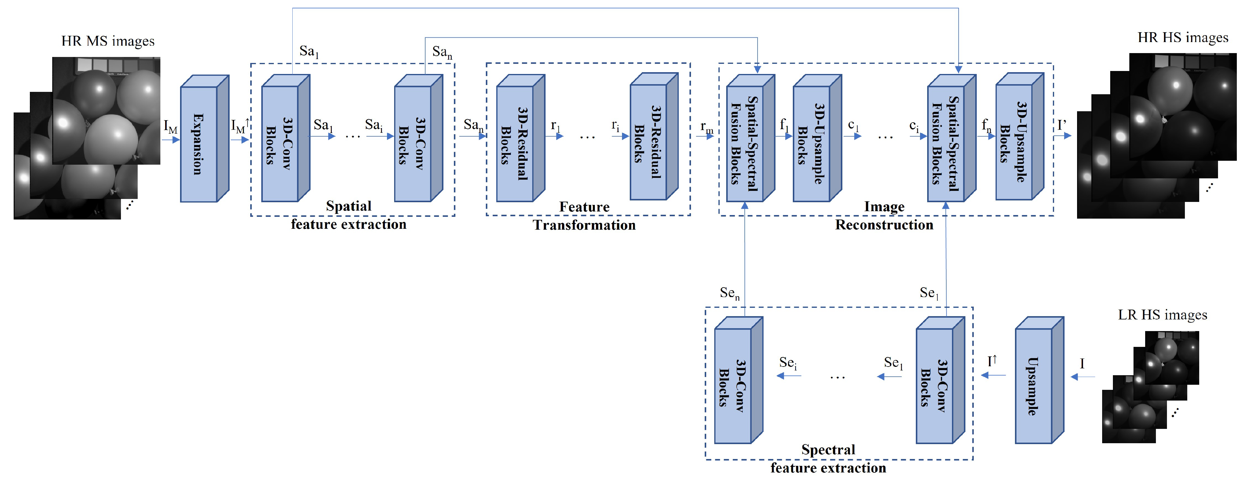
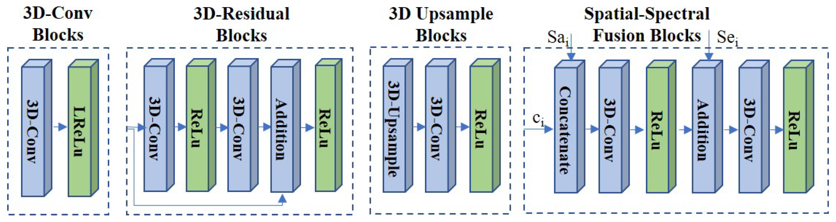
The architecture of the proposed network is shown in Figure 2, which depends on a modified and expanded version of U-Net [25]. With the input of LR HS images I and HR MS images , the proposed spectral super-resolution network (SSRN) G generates the resulting HR HS images (, where is the weight and bias parameters in the network G. These parameters are utilized while training and testing the network G. The LR HS images are upsampled using bicubic interpolation to have the same spatial size as the HR MS images. The HR MS images are expanded using the duplication operation, and the expanded HR HS images contain the same spectral channels as the HR HS images. The proposed neural network employs a 3D CNN considering spatial and spectral correlation simultaneously with thespectral super-resolution of the HR MS images. We constructed the 3D encoder–decoder framework, which encodes the spatial and spectral feature and decodes the fused spatial–spectral feature to reconstruct the result HS images. The SSR network consists of three parts: spatial/spectral feature extraction, feature transform, and image reconstruction. The spatial/spectral feature extraction (SFE) network introduces the 3D-Conv blocks to extract the spatial and spectral features from the HR MS and LR HS images. The feature transform (FT) network employs 3D-residual blocks in the middle network and transforms the features to prepare for pansharpened image reconstruction. The image reconstruction (IR) network mainly generates the spectrally enhanced images from the extracted spatial, spectral, and reconstruction features. It consists of two architectures: spatial and spectral fusion (SSF) blocks and 3D upsampling blocks. The former one is developed to fuse the extracted spatial feature and spectral features with the reconstruction features in each layer. The latter one is employed to reconstruct the resulting images with enhanced spatial and spectral resolutions. We summarize the sub-neural network block of the proposed network as follows (see the Figure 3):
- The 3D-Conv blocks: In the SFE network, we employed the 3D-Conv blocks with the kernel size of and stride of . Then, the leaky rectified linear unit (LReLU) activation is used. The 3D-Conv block is introduced to extract the spatial–spectral feature and from HR MS image and LR HS image I.
- The 3D residual blocks: In the FT network, 3D residual blocks are used to learn the extracted feature more efficiently in deep layers via residual learning [26]. In each block, we applied the 3D-Conv blocks with a kernel size of and stride of . The ReLU layers are utilized as the output layer. The addition layer is employed to concatenate the input feature and the learned residual feature.
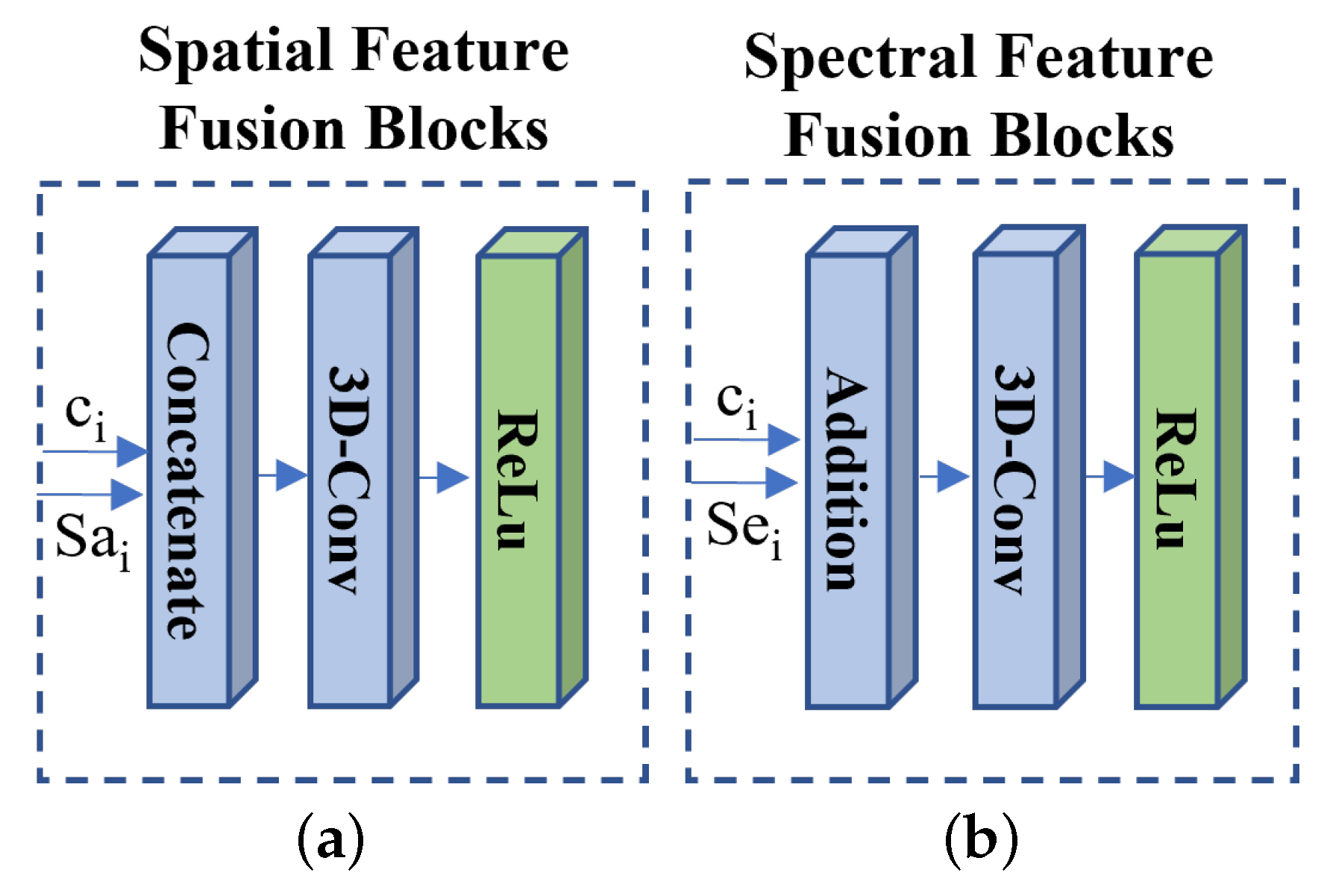
- The spatial–spectral fusion (SSF) blocks: In the image reconstruction network, the SSF blocks with a set of skip connections are utilized to fuse the reconstructed feature with the extracted spatial feature and the spectral feature efficiently. It can overcome the extracted feature distortion in the feature transform network. We utilized the concatenate operation and addition operation to fuse the spatial feature and the spectral feature respectively. We employed the 3D-Conv layer (kernel size: and stride: ) with the ReLU activation to transform the fused feature.
- The 3D upsample blocks: After the SSF blocks, we introduced the 3D upsample blocks to increase the spatial and spectral resolution. In each block, the 3D upsample layer with the nearest neighbor interpolation is first applied to generate the upsampled feature with enhanced spatial and spectral resolution. Then, the 3D-Conv layer (kernel size: and stride: ) with the ReLU activation is employed to generate the reconstructed feature . The 3D upsample blocks are applied to provide the spatial and spectral super-resolution of the reconstructed feature and obtain the resulting images .
3.3. Loss Function
Designing a suitable loss function is most important to improve the performance of the proposed neural network. The proposed loss function was developed to preserve the spatial and spectral content from the ground truth HS images. The sharp structure of HR MS images can be transferred to the generated HS images considering the spatial and spectral discrepancy between two images. We define the loss function, which consists of three parts, as follows:
- (1)
- Pixel loss: The pixel loss function enforces the pixel intensity consistency (content loss), which is defined as the -norm between the reconstructed image and the ground truth :where i, j, and k are the pixel location in the image. The -norm has been widely used in super-resolution with less blurring results compared to the -norm [27].
- (2)
- Spatial–spectral gradient (SSG) loss: To enforce the gradient consistency in terms of the spatial and spectral domains from the ground truth, we designed the 3D spatial–spectral gradient loss using the -norm as follows:where , , and are the gradient operators (i.e., forward difference operator) to obtain the x-, y-, and z-direction gradients of images. is the ground truth HS image. This loss can preserve the spatial and spectral gradients from the ground truth HS images. and measure the spatial gradient consistency estimation between the reconstructed HS images and HR MS images (we mention them in the next section).
- (3)
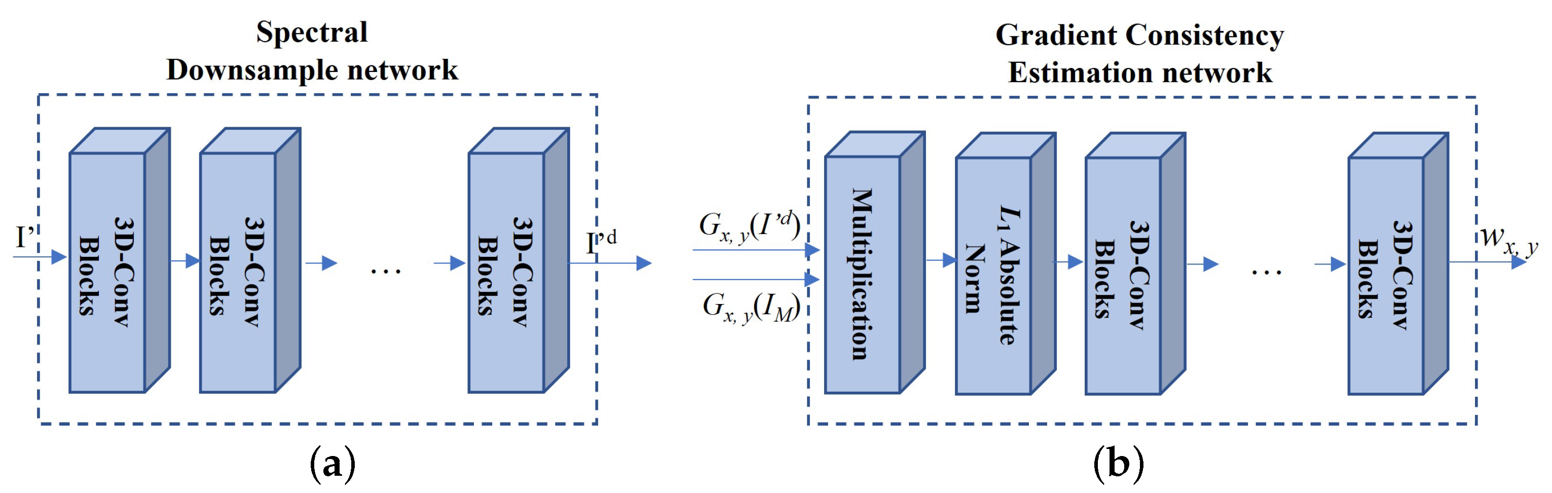
- Deep gradient transfer (DGT) loss: deep gradient transfer loss is designed to transfer the structure of HR MS images to the reconstructed HS images. However, HS and MS images have a large discrepancy in the spatial gradient and spectral channels. To overcome the spatial and spectral discrepancy, the GCE net and SD net are utilized while transferring the structure of the HR MS images. The DGT loss is designed as follows:where is the spectral downsampled version of the reconstructed HS images. It is generated by , which is the spectral downsample network (SD network) (see Figure 4) with several 3D-Conv blocks (see the left subfigure in Figure 3) (kernel size: (3, 3, 3) and stride: (1, 1, 2)). The output images have the same spectral channels as the HR MS images. To tackle the spatial discrepancy, the deep spatial gradient consistency (i.e., and ) between the spectral downsampled HS images and HR MS images is estimated as follows:where is the gradient consistency estimation (GCE) network with one multiplication operation, one absolute norm operation, and several 3D-Conv blocks (see the right subfigure in Figure 4) (kernel size: (3, 3, 3) and the stride: (1, 1, 1)). The multiplication operation is utilized to obtain the consistency gradient of the downsampled HS images and the HR MS images. Then, the absolute norm of the consistency gradient is obtained. Finally, the convolution symbol is included in the GCE network, which learns the consistency structure from the multiplication of the two image gradients. is the weight of the output of GCE network and is set to 10 in the proposed method.
The GCE network was developed to learn the gradient consistency between two images, and then, the HR MS image gradient is selectively transferred based on the gradient consistency. A large gradient consistency value (i.e., and ) means two images have the consistency gradient, and thus, the proposed method provides the strong HR MS image gradient transfer to the reconstructed HS images. On the contrary, a small spatial gradient consistency value enforces the spatial gradient preservation from the ground truth HS images. Thus, we assign and as the DGT loss and SSG loss. Finally, the 2D spatial gradient losses ( and are the same as those in Equation (4)) are applied to constrain the spatial gradient consistency between the HR MS images and the reconstructed HS images.
4. Experiments
In this section, we conduct the experiments on the public hyperspectral datasets to evaluate the superior performance of the proposed method. The compared methods are coupled nonnegative matrix factorization unmixing (CNMF) for pansharpening [28], RFuse [29], detail injection-based deep convolutional neural networks for pansharpening (DI-DCNN) [30], and MS/HS fusion net (MHF net) [31]. The former two methods are traditional methods, and the latter two methods are deep learning methods. We implemented the proposed method in tensorflow 2.0 and trained it on the Geforce RTX 2080Ti. In our experiments, we trained the network by using the Adam optimizer with the initial learning rate of . The iteration number was 200,000, and the batch size was 10. The slope of the leakyReLU activation was in all activation layers. To obtain the best performance of the proposed method, we set , , for the CAVE dataset, set , , for the Chikusei dataset, and set , , for the WV2 dataset. The three datasets are mentioned in the Section 4.1.
4.1. Dataset and Evaluation Metrics
In the experiments, we used three hyperspectral datasets. These are the CAVE Multispectral Image dataset [22], Chikusei dataset [23], and World View-2 dataset (https://www.harrisgeospatial.com/DataImagery/SatelliteImagery/HighResolution/WorldView-2.aspx, accessed on 13 August 2021):
- (1)
- CAVE dataset: The CAVE dataset consists of 32 images with a spatial size of and the total spectral channels of 31 bands. The band range is from 400 nm to 700 nm. The size of the HR MS image is . The first 20 images were set as the training data, and we randomly cropped the patches from each HS image as the ground truth, i.e., HR HS images. The LR HS images were generated by downsampling the ground truth HS images by a factor of 4. The average operation over was used in the downsampling operation, which refers to [31]. Thus, the training HR HS, HR MS, and LR MS images had a size of , , and . We utilized the remaining 12 images as the test data. The LR HS images and the HR HS images were utilized as the input and the ground truth.
- (2)
- Chikusei dataset: The Chikusei dataset (http://naotoyokoya.com/Download.html, accessed on 20 August 2020) is airborne HS images captured over Chikusei on 29 July 2014 [23]. The size of the HR HS image is and the size of the HR MS image is . The band range is from 363 nm to 1018 nm. We selected the top-left portion with a size of as the training data, and the remaining parts were treated as the test data. The training and test datasets were generated like the CAVE dataset. The training HR HS, HR MS, and LR HS images had a size of , , and . During the test procedure, we extracted 16,320 -spatial-size patches from the test data of HR HS and HR MS images. The HR HS patches were employed as the ground truth, and the LR HS patches were generated as the input.
- (3)
- World View-2 (WV-2) dataset: The World View-2 dataset is a real dataset consisting of LR multispectral images with a size of and HR panchromatic images with a size of . We employed the Wald protocol [32] to prepare the training samples for the real data. We treated the LR multispectral images as the HR HS images and downsampled the HR panchromatic images by a factor of 4. The downsampled HR panchromatic images were considered as the HR MS images. We utilized the top portion (size: ) of the HR HS and HR MS images as the training data and the remaining part as the test data. As with the CAVE dataset, the extracted training HR HS, HR MS, and LR HS patches are , , and . In the test data, we extracted -spatial-size patches from the test data of the HR HS and HR MS images. The HR HS patches were employed as the ground truth, and the LR HS patches were generated as the input.
The network structure of the three datasets is illustrated in Table 2. Because the three datasets had different spectral numbers in the images, we utilized the same network structure with different layer numbers. To better extract the spatial and spectral features, we provided the deeper layers to the images with more spectral channels. In Figure 3, the kernel size and stride of the 3D-Conv layers are and in 3D-Conv blocks. The kernel size and stride of the 3D-Conv layers are and in the 3D residual blocks, 3D upsample blocks, and SSF blocks.
To evaluate the performance of the compared methods, in addition to the subjective evaluation, five evaluation indexes were employed. These are the peak-signal-to-noise ratio (PSNR), structural similarity (SSIM) [33], spectral angle mapper (SAM) [34], Erreur Relative Globale Adimensionnelle de Synthése (ERGAS) [35], and Q2N [36]. The PSNR metric is the traditional image quality index, which estimates the spatial quality of the reconstructed image using the mean-squared error. The SSIM metric evaluates the structural similarity between the ground truth and the reconstructed image. The SAM assesses the spectral distortion by calculating the average angle between the spectral vectors of the generated HS images and the ground truth. The SAM is formulated as follows:
where arccos is the arc-cosine function. The ERGAS measures the overall fused image quality based on the downsampling ratio, which is calculated as
where d is the spatial downsampling factor. is the mean value of in the band k. is the mean-squared difference between the result and the ground truth . The Q2N metric [36] reflects the image quality with the computation of the hypercomplex correlation coefficient between the result and the ground truth in the spectral and spatial domains. Smaller SAM and ERGAS values mean better spectral preservation of the HS images. Larger PSNR values report better image fidelity in the spatial domain. Larger SSIM values mean more structure similarity between the result and the ground truth. Q2N values reflect better spectral and spatial correlation between the ground truth and the reconstruction results.
4.2. Comparison to State-of-the-Art
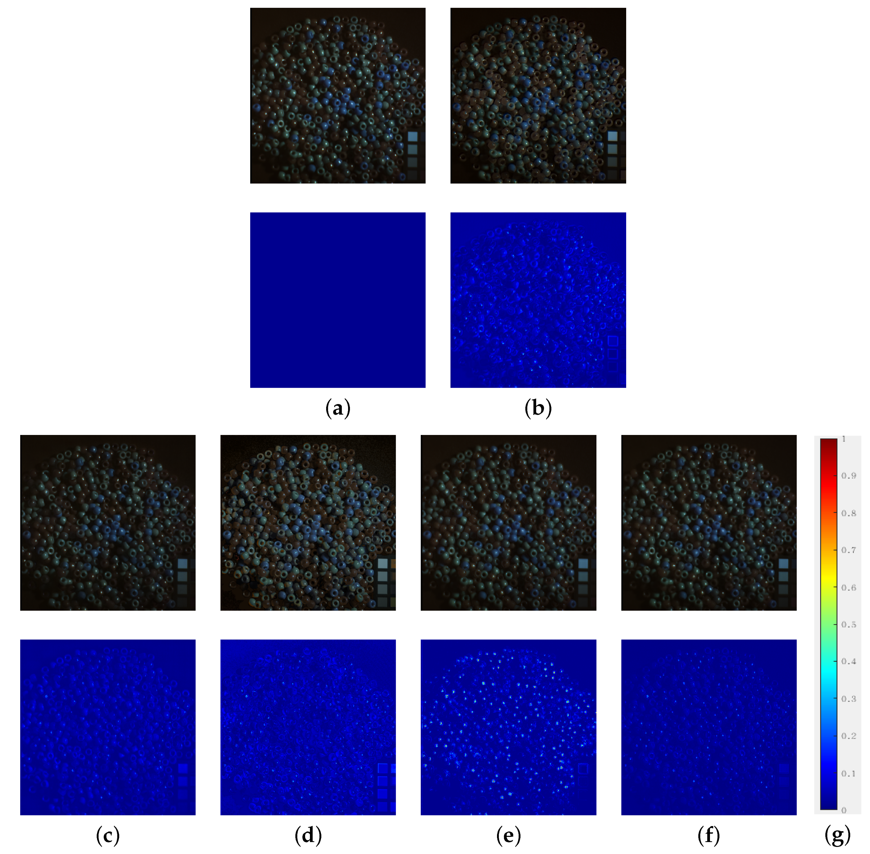
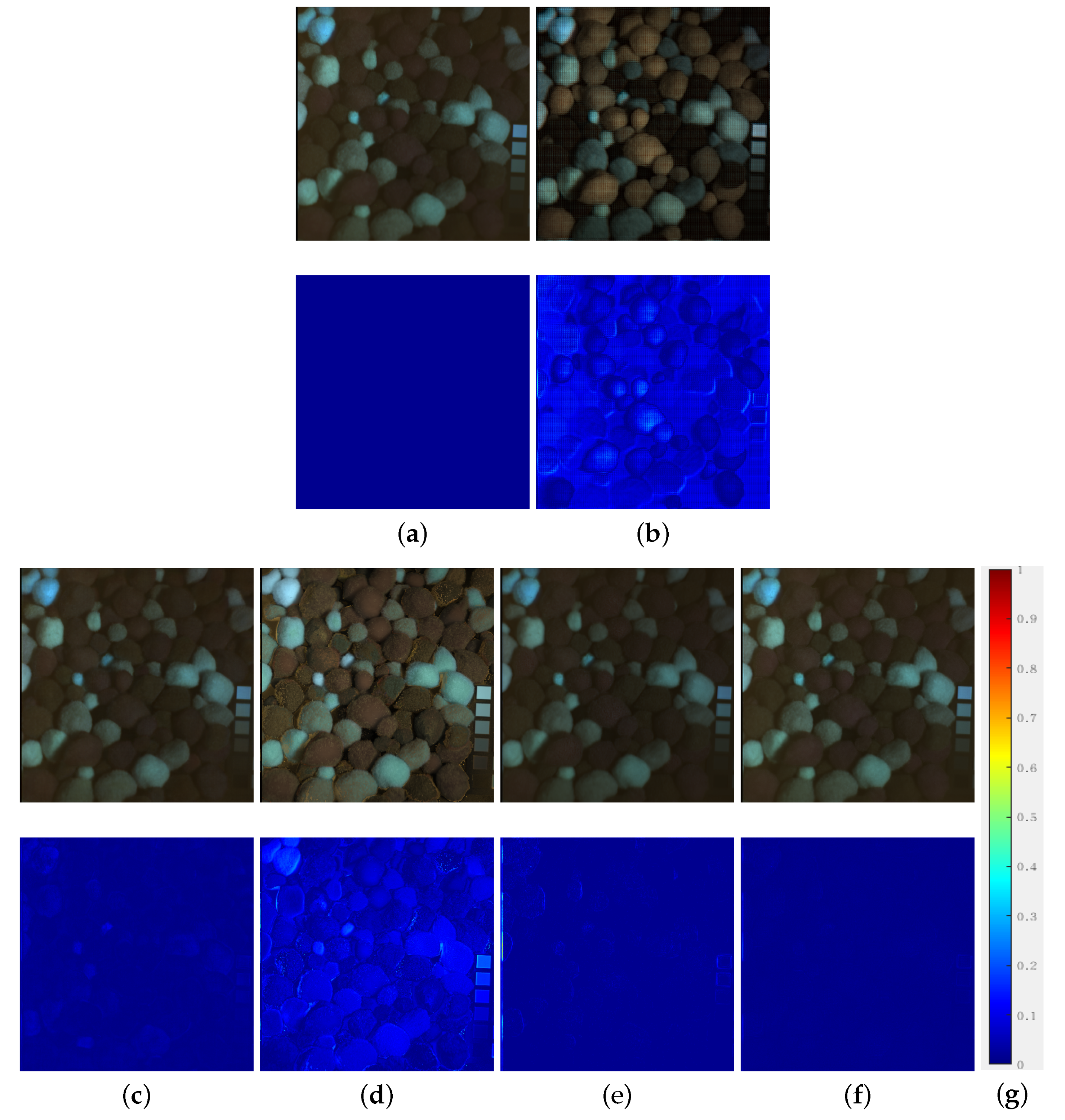
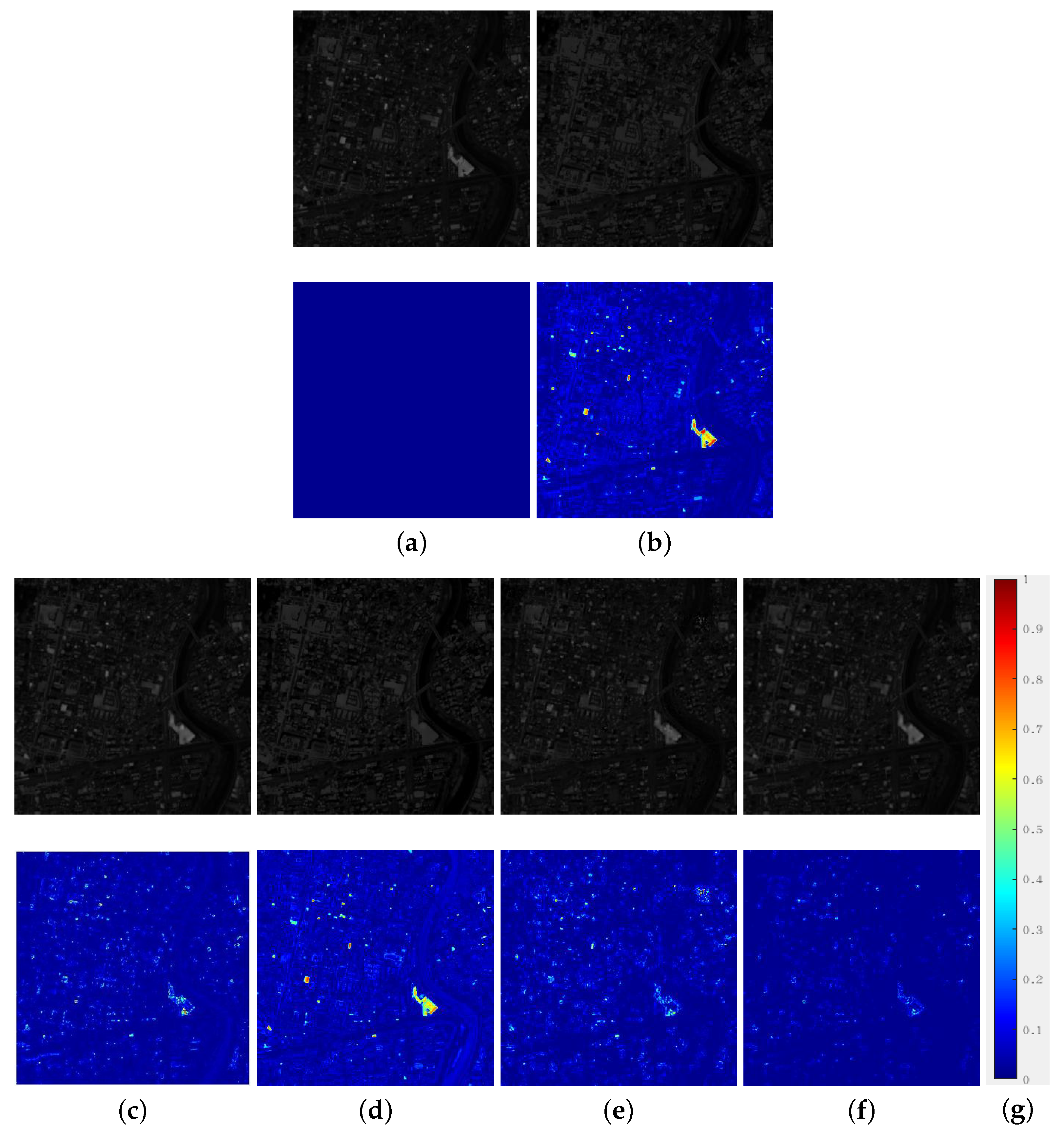
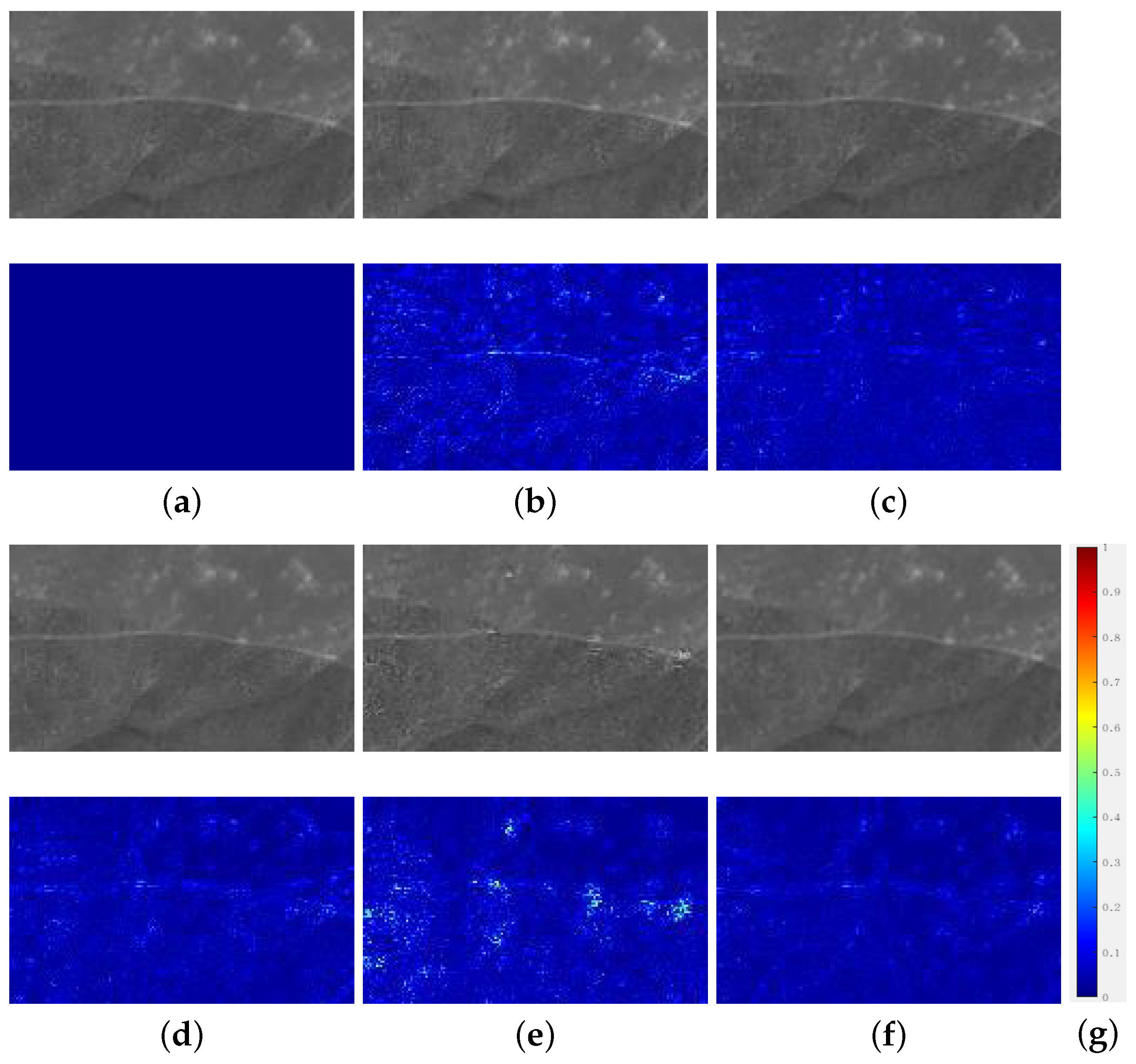
Figure 5 and Figure 6 show the results of five compared methods on the CAVE dataset. In terms of subjective results, the proposed, MHF, and DI-DCNN methods generated visually similar results to the ground truth (see the first row in Figure 5 and Figure 6c,e,f). From the absolute difference map (see the second row of the figures), the proposed method produced results with the least difference compared to MHF and DI-DCNN. Figure 7 and Figure 8 show the results on the Chikusei and WV2 datasets. As for the CAVE datasets, the proposed method generated results with the least difference among the five compared methods (see the second row in the figures). Thus, the proposed method achieves the best performance in subjective results.
Table 3, Table 4 and Table 5 show the objective evaluation of the five compared methods on the CAVE, Chikusei, and WV2 datasets. The proposed method achieved the best performance in the SSIM, SAM, ERGAS, and PSNR among the three datasets. In the Q2N metric, the proposed method obtained the best performance on the Chikusei and WV2 datasets, but obtained slightly worse performance compared to DI-DCNN on the CAVE dataset. It is shown that the proposed method generates the results with good performance in structure and spectral preservation from the ground truth.
4.3. Model Analysis
4.3.1. Loss Function
Table 6 reports the objective evaluation of the proposed method with different loss functions. and do not consider the spatial discrepancy (i.e., we removed the weight of Equations (4) and (5)). The loss functions are rewritten as Equations (10) and (11).
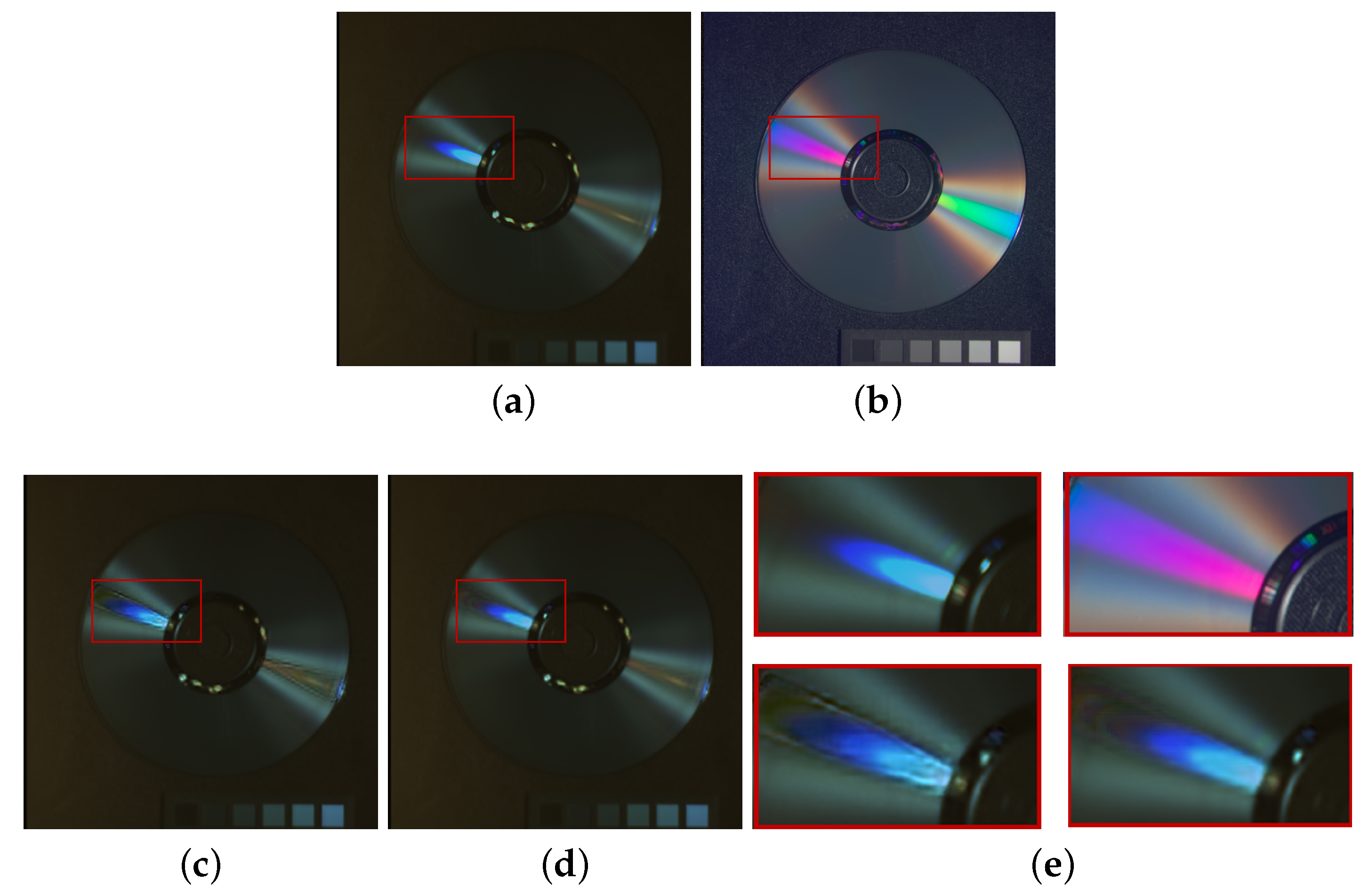
enforces the spatial and spectral structure consistency between the results and the ground truth. Thus, had better performance compared to in the objective assessment. With additional employment of the DGT loss, achieved a slightly worse performance because a large spatial discrepancy leads to the gradient distortion in the reconstructed HS images (see the red blocks in Figure 9). Therefore, considering the spatial discrepancy (GCE net in Figure 4), the proposed method achieved the best performance among the four loss functions.
4.3.2. Component Analysis
This section analyzes the effect of the spatial feature fusion and spectral feature fusion in the SSF blocks. We utilized different network structures of the spatial–spectral fusion (SSF) block for this experiment. The experiments analyzed the effect of spatial feature fusion, spectral feature fusion, and both features’ fusion. The different network structures are shown in Figure 10 and the rightmost figure of Figure 4. These networks should be retrained. Table 7 shows the objective evaluation of the results generated by the spatial feature fusion, spectral feature fusion, and both features’ fusion. Figure 11 shows the visual results by the spatial fusion, spectral fusion, and both features’ fusion. It is shown that the proposed method with both feature’s fusion preserves more spatial and spectral information from the ground truth (see Figure 11c,d). Table 7 also validates that the proposed method with both features’ fusion achieves the best performance in the objective evaluation.
4.4. Compared to 2D Convolutional Neural Network
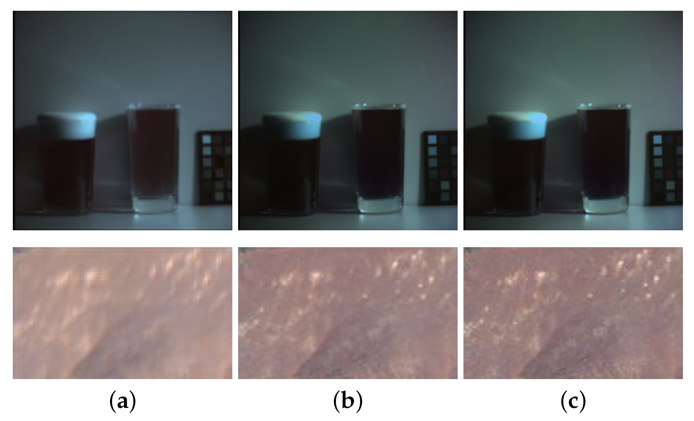
This section compares the performance of the 2D CNN and 3D CNN in the proposed method. Figure 12 shows that the results of the 2D CNN and 3D CNN. It is seen that the 3D CNN considers the spectral correlation and generates a results with spectral information more similar to the ground truth (see the similar colors in Figure 12b,c). It is shown that the the proposed method by the 3D CNN provides better performance compared to the 2D CNN.
4.5. Extension to Different Downsampling Factors
In the previous section, we conducted the experiments on the corresponding LR HS images with a downsampling factor of four. Here, we provide the objective experiments of the compared methods on different downsampling factors. Table 8 and Table 9 represent the average objective evaluation of the five compared methods with downsampling factors of and . We utilized the five objective evaluations of the SSIM, SAM, ERGAS, PSNR, and Q2N metrics for the experiment. With the increase of the downsampling factors, it is shown that the proposed method achieved the best performance among the compared methods in terms of the five objective metrics.
5. Conclusions
In this paper, we proposed a novel supervised pansharpening network, which was designed as the spectral super-resolution framework. The network consists of three stages: spectral/spatial feature extraction, feature transformation, and image reconstruction. We designed the SSF blocks, which reuse the extracted feature in the image reconstruction. The DDHG losses were developed to preserve the spatial and spectral features from the HR MS and HR HS images considering the spatial and spectral discrepancy between two images. The experimental results showed that the proposed method achieved the best performance in the subjective and objective evaluation of the spectral and spatial preservation among state-of-the-art methods.
Author Contributions
Conceptualization, H.S. and H.J.; methodology, H.S.; software, H.S.; validation, H.S. and H.J.; formal analysis, H.S.; investigation, H.S.; resources, H.S.; data curation, H.S. and C.S.; writing—original draft preparation, H.S.; writing—review and editing, H.S., H.J. and C.S.; visualization, H.S.; supervision, H.S.; project administration, H.S. and H.J.; funding acquisition, H.S. All authors have read and agreed to the published version of the manuscript.
Funding
This research was funded by the Natural Science Basic Research Program of ShaanXi (Program No. 2022JQ-647).
Data Availability Statement
Not applicable.
Acknowledgments
The authors would like to thank the Editors and the anonymous Reviewers for their comments and suggestions.
Conflicts of Interest
The authors declare on conflict of interest.
References
- Lin, C.; Chen, S.Y.; Chen, C.C.; Tai, C.H. Detecting Newly Grown Tree Leaves from Unmanned-Aerial-Vehicle Images using Hyperspectral Target Detection Techniques. ISPRS J. Photogramm. Remote Sens. 2018, 142, 174–189. [Google Scholar] [CrossRef]
- Yuan, Q.; Zhang, Q.; Li, J.; Shen, H.; Zhang, L. Hyperspectral Image Denoising Employing a Spatial–Spectral Deep Residual Convolutional Neural Network. IEEE Trans. Geosci. Remote Sens. 2019, 57, 1205–1218. [Google Scholar] [CrossRef]
- Mei, S.; Ji, J.; Geng, Y.; Zhang, Z.; Li, X.; Du, Q. Unsupervised Spatial–Spectral Feature Learning by 3D-Convolutional Autoencoder for Hyperspectral Classification. IEEE Trans. Geosci. Remote Sens. 2019, 57, 6808–6820. [Google Scholar] [CrossRef]
- Xie, J.; He, N.; Fang, L.; Ghamisi, P. Multiscale Densely-Connected Fusion Networks for Hyperspectral Images Classification. IEEE Trans. Circuits Syst. Video Technol. 2021, 31, 246–259. [Google Scholar] [CrossRef]
- Shettigara, V.K. A generalized component substitution technique for spatial enhancement of multispectral images using a higher resolution data set. Photogramm. Eng. Remote Sens. 1992, 58, 561–567. [Google Scholar]
- Xu, Y.; Wu, Z.; Chanussot, J.; Wei, Z. Hyperspectral Computational Imaging via Collaborative Tucker3 Tensor Decomposition. IEEE Trans. Circuits Syst. Video Technol. 2021, 31, 98–111. [Google Scholar] [CrossRef]
- Vivone, G.; Restaino, R.; Mura, M.D.; Licciardi, G.; Chanussot, J. Contrast and Error-Based Fusion Schemes for Multispectral Image Pansharpening. IEEE Geosci. Remote Sens. Lett. 2014, 11, 930–934. [Google Scholar] [CrossRef]
- Aiazzi, B.; Alparone, L.; Baronti, S.; Garzelli, A.; Selva, M. MTF-tailored multiscale fusion of high-resolution MS and pan imagery. Photogramm. Eng. Remote Sens. 2006, 72, 591–596. [Google Scholar] [CrossRef]
- Choi, J.; Park, H.; Seo, D. Pansharpening Using Guided Filtering to Improve the Spatial Clarity of VHR Satellite Imagery. Remote Sens. 2019, 11, 633. [Google Scholar] [CrossRef]
- Fasbender, D.; Radoux, J.; Bogaert, P. Bayesian Data Fusion for Adaptable Image Pansharpening. IEEE Trans. Geosci. Remote Sens. 2008, 46, 1847–1857. [Google Scholar] [CrossRef]
- Chen, C.; Li, Y.; Liu, W.; Huang, J. Image Fusion with Local Spectral Consistency and Dynamic Gradient Sparsity. In Proceedings of the 2014 IEEE Conference on Computer Vision and Pattern Recognition, Washington, DC, USA, 23–28 June 2014; pp. 2760–2765. [Google Scholar]
- Wang, T.; Fang, F.; Li, F.; Zhang, G. High-Quality Bayesian Pansharpening. IEEE Trans. Image Process. 2019, 28, 227–239. [Google Scholar] [CrossRef]
- Masi, G.; Cozzolino, D.; Verdoliva, L.; Scarpa, G. Pansharpening by Convolutional Neural Networks. Remote Sens. 2016, 8, 594. [Google Scholar] [CrossRef]
- Shao, Z.; Cai, J. Remote Sensing Image Fusion with Deep Convolutional Neural Network. IEEE J. Sel. Top. Appl. Earth Obs. Remote Sens. 2018, 11, 1656–1669. [Google Scholar] [CrossRef]
- Li, K.; Xie, W.; Du, Q.; Li, Y. DDLPS: Detail-Based Deep Laplacian Pansharpening for Hyperspectral Imagery. IEEE Trans. Geosci. Remote Sens. 2019, 57, 8011–8025. [Google Scholar] [CrossRef]
- Dian, R.; Li, S.; Guo, A.; Fang, L. Deep Hyperspectral Image Sharpening. IEEE Trans. Neural Netw. Learn. Syst. 2018, 29, 5345–5355. [Google Scholar] [CrossRef]
- Xie, W.; Lei, J.; Cui, Y.; Li, Y.; Du, Q. Hyperspectral Pansharpening with Deep Priors. IEEE Trans. Neural Netw. Learn. Syst. 2020, 31, 1529–1543. [Google Scholar] [CrossRef]
- Wang, X.; Chen, J.; Wei, Q.; Richard, C. Hyperspectral Image Super-Resolution via Deep Prior Regularization with Parameter Estimation. IEEE Trans. Circuits Syst. Video Technol. 2021, 32, 1708–1723. [Google Scholar] [CrossRef]
- Luo, S.; Zhou, S.; Feng, Y.; Xie, J. Pansharpening via Unsupervised Convolutional Neural Networks. IEEE J. Sel. Top. Appl. Earth Obs. Remote Sens. 2020, 13, 4295–4310. [Google Scholar] [CrossRef]
- Zhou, C.; Zhang, J.; Liu, J.; Zhang, C.; Fei, R.; Xu, S. PercepPan: Towards Unsupervised Pan-Sharpening Based on Perceptual Loss. Remote Sens. 2020, 12, 2318. [Google Scholar] [CrossRef]
- Ozcelik, F.; Alganci, U.; Sertel, E.; Unal, G. Rethinking CNN-Based Pansharpening: Guided Colorization of Panchromatic Images via GANs. IEEE Trans. Geosci. Remote Sens. 2020, 59, 3486–3501. [Google Scholar] [CrossRef]
- Yasuma, F.; Mitsunaga, T.; Iso, D.; Nayar, S. Generalized Assorted Pixel Camera: Post-Capture Control of Resolution, Dynamic Range and Spectrum. Technical Report. 2008. Available online: http://citeseerx.ist.psu.edu/viewdoc/download?doi=10.1.1.360.7873&rep=rep1&type=pdf (accessed on 20 July 2022).
- Yokoya, N.; Iwasaki, A. Airborne Hyperspectral Data over Chikusei; Technical Report SAL-2016-05-27; Space Application Laboratory, University of Tokyo: Tokyo, Japan, 2016. [Google Scholar]
- Shannon, C.E. A mathematical theory of communication. ACM SIGMOBILE Mob. Comput. Commun. Rev. 2001, 5, 3–55. [Google Scholar] [CrossRef]
- Ronneberger, O.; Fischer, P.; Brox, T. U-Net: Convolutional Networks for Biomedical Image Segmentation. In MICCAI 2015, Proceedings of the Medical Image Computing and Computer-Assisted Intervention, Munich, Germany, 5–9 October 2015; Navab, N., Hornegger, J., Wells, W.M., Frangi, A.F., Eds.; Springer International Publishing: Cham, Switzerland, 2015; pp. 234–241. [Google Scholar]
- He, K.; Zhang, X.; Ren, S.; Sun, J. Deep Residual Learning for Image Recognition. In Proceedings of the 2016 IEEE Conference on Computer Vision and Pattern Recognition (CVPR), Las Vegas, NV, USA, 26 June–1 July 2016; pp. 770–778. [Google Scholar] [CrossRef]
- Xue, Y.; Xu, T.; Zhang, H.; Long, L.R.; Huang, X. SegAN: Adversarial Network with Multi-scale L1 Loss for Medical Image Segmentation. Neuroinformatics 2018, 16, 383–392. [Google Scholar] [CrossRef] [PubMed]
- Yokoya, N.; Yairi, T.; Iwasaki, A. Coupled Nonnegative Matrix Factorization Unmixing for Hyperspectral and Multispectral Data Fusion. IEEE Trans. Geosci. Remote Sens. 2012, 50, 528–537. [Google Scholar] [CrossRef]
- Wei, Q.; Dobigeon, N.; Tourneret, J.; Bioucas-Dias, J.; Godsill, S. R-FUSE: Robust Fast Fusion of Multiband Images Based on Solving a Sylvester Equation. IEEE Signal Process. Lett. 2016, 23, 1632–1636. [Google Scholar] [CrossRef]
- Deng, L.J.; Vivone, G.; Jin, C.; Chanussot, J. Detail Injection-Based Deep Convolutional Neural Networks for Pansharpening. IEEE Trans. Geosci. Remote Sens. 2021, 59, 6995–7010. [Google Scholar] [CrossRef]
- Xie, Q.; Zhou, M.; Zhao, Q.; Meng, D.; Zuo, W.; Xu, Z. Multispectral and Hyperspectral Image Fusion by MS/HS Fusion Net. In Proceedings of the 2019 IEEE/CVF Conference on Computer Vision and Pattern Recognition (CVPR), Long Beach, CA, USA, 15–20 June 2019; pp. 1585–1594. [Google Scholar]
- Wald, L.; Ranchin, T.; Mangolini, M. Fusion of satellite images of different spatial resolution: Assessing the quality of resulting images. Photogramm. Eng. Remote Sens. 1997, 63, 691–699. [Google Scholar]
- Zhou, W.; Bovik, A.C.; Sheikh, H.R.; Simoncelli, E.P. Image quality assessment: From error visibility to structural similarity. IEEE Trans. Image Process. 2004, 13, 600–612. [Google Scholar]
- Yuhas, R.H.; Goetz, A.B.J. Discrimination among semi-arid landscape endmembers using the spectral angle mapper (SAM) algorithm. In Proceedings of the Summaries 3rd Annual JPL Airborne Geoscience Workshop, Pasadena, CA, USA, 1–5 June 1992; Volume 1, pp. 147–149. [Google Scholar]
- Ranchin, T.; Wald, L. Fusion of high spatial and spectral resolution images: The ARSIS concept and its implementation. Photogramm. Eng. Remote Sens. 2000, 66, 49–61. [Google Scholar]
- Garzelli, A.; Nencini, F. Hypercomplex Quality Assessment of Multi/Hyperspectral Images. IEEE Geosci. Remote Sens. Lett. 2009, 6, 662–665. [Google Scholar] [CrossRef]
Figure 1.
Test image paints and chart and stuffed toy in the CAVE dataset. (a) MS image; (b) HS image at band 3; (c) HS image at band 27.
Figure 1.
Test image paints and chart and stuffed toy in the CAVE dataset. (a) MS image; (b) HS image at band 3; (c) HS image at band 27.

Figure 2.
Entire framework of the proposed method. The proposed spectral super-resolution network consists of three parts: spatial/spectral feature extraction, feature transformation, and image reconstruction. , , and are the spatial, spectral, and reconstructed feature from the input HR MS, LR HS, and reconstructed HR HS images. is the fusion feature after the spatial–spectral fusion blocks, and is the feature from the 3D residual blocks.

Figure 3.
The architecture of the sub-neural network blocks.

Figure 4.
The proposed spectral downsample network (a) and gradient consistency estimation network (b).
Figure 4.
The proposed spectral downsample network (a) and gradient consistency estimation network (b).

Figure 5.
Experimental results for test image beads at 1–3th band. (a) Ground truth; (b) RFuse [29]; (c) MHF [31]; (d) CNMF [28]; (e) DI-DCNN [30]; (f) proposed method; (g) error illustration of the absolute difference map. The first row shows the results of the compared methods; the second row shows the absolute difference map between the results and the ground truth.

Figure 6.
Experimental results for test image pompoms at the 1–3th band. (a) Ground truth; (b) RFuse [29]; (c) MHF [31]; (d) CNMF [28]; (e) DI-DCNN [30]; (f) proposed method; (g) error illustration of the absolute difference map. The first row shows the results of the compared methods; the second row shows the absolute difference map between the results and the ground truth.

Figure 7.
Experimental results for test image Chikusei at the 45th band. (a) Ground truth; (b) RFuse [29]; (c) MHF [31]; (d) CNMF [28]; (e) DI-DCNN [30]; (f) proposed method; (g) error illustration of the absolute difference map. The first row shows the results of the compared methods; the second row shows the absolute difference map between the results and the ground truth.

Figure 8.
Experimental results for test image WV-2 at the 4th band. (a) Ground truth; (b) RFuse [29]; (c) MHF [31]; (d) CNMF [28]; (e) DI-DCNN [30]; (f) proposed method; (g) error illustration of the absolute difference map. The first row shows the results of the compared methods; the second row shows the absolute difference map between the results and the ground truth.

Figure 9.
Experimental results for test image cds with different loss functions. (a) Ground truth; (b) HR MS images; (c) ; (d) ; (e) zoomed regions of the red blocks (top-left: (a), top-right: (b), bottom-left: (c) and bottom-right: (d)).
Figure 9.
Experimental results for test image cds with different loss functions. (a) Ground truth; (b) HR MS images; (c) ; (d) ; (e) zoomed regions of the red blocks (top-left: (a), top-right: (b), bottom-left: (c) and bottom-right: (d)).

Figure 10.
The network architecture of (a) spatial feature fusion blocks and (b) spectral feature fusion blocks.
Figure 10.
The network architecture of (a) spatial feature fusion blocks and (b) spectral feature fusion blocks.

Figure 11.
Comparison of different model components in the proposed method on the CAVE and WV2 datasets. (a) Spatial feature fusion; (b) spectral feature fusion; (c) both features’ fusion; (d) ground truth.
Figure 11.
Comparison of different model components in the proposed method on the CAVE and WV2 datasets. (a) Spatial feature fusion; (b) spectral feature fusion; (c) both features’ fusion; (d) ground truth.

Figure 12.
Comparison of the 2D CNN and 3D CNN in the proposed methods on the CAVE and WV2 datasets: (a) 2D CNN; (b) 3D CNN; (c) ground truth.
Figure 12.
Comparison of the 2D CNN and 3D CNN in the proposed methods on the CAVE and WV2 datasets: (a) 2D CNN; (b) 3D CNN; (c) ground truth.


Table 1.
DE evaluation of the CAVE and Chikusei datasets.
| Dataset | CAVE | Chikusei |
|---|---|---|
| HR MS images | 6.41 | 7.07 |
| HR HS images | 5.21 | 4.58 |
Table 2.
Network architecture of the proposed spectral super-resolution on the three datasets.
| Datasets | CAVE | Chikusei | WV2 |
|---|---|---|---|
| SFE Net | 3 × 3D-Conv | 5 × 3D-Conv | 2 × 3D-Conv |
| FT Net | 8 × 3D-Residual | 8 × 3D-Residual | 8 × 3D-Residual |
| IR Net | 3 × SSF + 3 × 3D Upsample | 5 × SSF + 5 × 3D Upsample | 2 × SSF + 2 × 3D Upsample |
| SD Net | 3 × 3D-Conv | 5 × 3D-Conv | 2 × 3D-Conv |
| GCE Net | 2 × 3D-Conv | 2 × 3D-Conv | 2 × 3D-Conv |
Table 3.
Quantitative measurement of the experimental results on the CAVE dataset. The best scores are highlighted in bold font.
Table 3.
Quantitative measurement of the experimental results on the CAVE dataset. The best scores are highlighted in bold font.
| Methods | SSIM | SAM | ERGAS | PSNR | Q2N |
|---|---|---|---|---|---|
| RFuse | 0.840 | 17.233 | 10.528 | 30.947 | 0.853 |
| MHF | 0.973 | 8.741 | 3.485 | 40.590 | 0.939 |
| CNMF | 0.903 | 16.106 | 9.606 | 31.703 | 0.844 |
| DI-DCNN | 0.975 | 8.585 | 3.906 | 42.648 | 0.946 |
| Proposed | 0.989 | 4.416 | 2.158 | 43.034 | 0.940 |
Table 4.
Quantitative measurement of the experimental results on the Chikusei dataset. The best scores are highlighted in bold font.
Table 4.
Quantitative measurement of the experimental results on the Chikusei dataset. The best scores are highlighted in bold font.
| Methods | SSIM | SAM | ERGAS | PSNR | Q2N |
|---|---|---|---|---|---|
| RFuse | 0.794 | 7.568 | 7.300 | 29.015 | 0.770 |
| MHF | 0.834 | 3.006 | 4.087 | 35.629 | 0.932 |
| CNMF | 0.677 | 4.882 | 7.238 | 29.417 | 0.772 |
| DI-DCNN | 0.778 | 4.144 | 5.704 | 31.450 | 0.872 |
| Proposed | 0.884 | 2.416 | 3.319 | 37.152 | 0.951 |
Table 5.
Quantitative measurement of the experimental results on the WV-2 dataset. The best scores are highlighted in bold font.
Table 5.
Quantitative measurement of the experimental results on the WV-2 dataset. The best scores are highlighted in bold font.
| Methods | SSIM | SAM | ERGAS | PSNR | Q2N |
|---|---|---|---|---|---|
| RFuse | 0.949 | 1.082 | 0.949 | 32.933 | 0.870 |
| MHF | 0.955 | 0.958 | 1.021 | 32.195 | 0.777 |
| CNMF | 0.951 | 1.015 | 0.869 | 33.714 | 0.883 |
| DI-DCNN | 0.871 | 1.850 | 1.853 | 30.660 | 0.718 |
| Proposed | 0.968 | 0.780 | 0.684 | 35.847 | 0.920 |
Table 6.
Average objective results of different losses on the three datasets. and do not consider the spatial discrepancy (i.e., ) by GCE net in Figure 4. includes all losses with GCE net. The best scores are highlighted in bold font.
Table 6.
Average objective results of different losses on the three datasets. and do not consider the spatial discrepancy (i.e., ) by GCE net in Figure 4. includes all losses with GCE net. The best scores are highlighted in bold font.
| Dataset | Loss | SSIM | SAM | ERGAS | PSNR | Q2N |
|---|---|---|---|---|---|---|
| CAVE | 0.980 | 6.200 | 2.935 | 40.310 | 0.920 | |
| 0.984 | 5.840 | 2.608 | 41.595 | 0.926 | ||
| 0.981 | 5.774 | 2.837 | 40.685 | 0.924 | ||
| 0.989 | 4.416 | 2.158 | 43.034 | 0.940 | ||
| Chikusei | 0.716 | 6.031 | 6.828 | 31.604 | 0.868 | |
| 0.876 | 2.538 | 3.991 | 36.814 | 0.946 | ||
| 0.830 | 3.636 | 4.291 | 35.234 | 0.925 | ||
| 0.884 | 2.416 | 3.319 | 37.152 | 0.951 | ||
| WV-2 | 0.962 | 0.853 | 0.748 | 35.167 | 0.908 | |
| 0.967 | 0.797 | 0.687 | 35.821 | 0.919 | ||
| 0.967 | 0.792 | 0.694 | 35.746 | 0.918 | ||
| 0.968 | 0.780 | 0.684 | 35.847 | 0.920 |
Table 7.
Average objective results of different model structures on the three datasets. The best scores are highlighted in bold font. Comp. represents component.
Table 7.
Average objective results of different model structures on the three datasets. The best scores are highlighted in bold font. Comp. represents component.
| Dataset | Comp. | SSIM | SAM | ERGAS | PSNR | Q2N |
|---|---|---|---|---|---|---|
| CAVE | Spa | 0.734 | 31.449 | 13.767 | 27.374 | 0.831 |
| Spe | 0.978 | 5.262 | 3.123 | 39.700 | 0.915 | |
| Spa + Spe | 0.989 | 4.416 | 2.158 | 43.034 | 0.940 | |
| Chikusei | Spa | 0.555 | 11.204 | 13.444 | 26.855 | 0.708 |
| Spe | 0.716 | 3.483 | 6.533 | 31.059 | 0.861 | |
| Spa + Spe | 0.884 | 2.416 | 3.319 | 37.152 | 0.951 | |
| WV2 | Spa | 0.888 | 2.763 | 1.737 | 29.013 | 0.752 |
| Spe | 0.964 | 0.803 | 0.720 | 35.412 | 0.912 | |
| Spa + Spe | 0.968 | 0.780 | 0.684 | 35.847 | 0.920 |
Table 8.
Average objective evaluation of the five compared methods on the three datasets with a downsampling factor. The best scores are highlighted in bold font.
Table 8.
Average objective evaluation of the five compared methods on the three datasets with a downsampling factor. The best scores are highlighted in bold font.
| Dataset | Methods | SSIM | SAM | ERGAS | PSNR | Q2N |
|---|---|---|---|---|---|---|
| CAVE | RFuse | 0.585 | 28.925 | 4.070 | 24.030 | 0.818 |
| MHF | 0.791 | 13.337 | 2.744 | 30.219 | 0.793 | |
| CNMF | 0.878 | 10.797 | 6.194 | 31.223 | 0.799 | |
| DI-DCNN | 0.852 | 11.843 | 3.900 | 27.547 | 0.809 | |
| Proposed | 0.961 | 8.314 | 1.268 | 35.701 | 0.893 | |
| Chikusei | RFuse | 0.737 | 12.297 | 10.740 | 26.354 | 0.391 |
| MHF | 0.945 | 3.863 | 4.980 | 32.563 | 0.991 | |
| CNMF | 0.784 | 5.936 | 8.153 | 28.516 | 0.350 | |
| DI-DCNN | 0.885 | 6.126 | 9.923 | 27.676 | 0.974 | |
| Proposed | 0.951 | 3.649 | 4.870 | 32.770 | 0.994 | |
| WV-2 | RFuse | 0.911 | 2.005 | 1.381 | 30.152 | 0.791 |
| MHF | 0.955 | 1.458 | 1.021 | 32.990 | 0.777 | |
| CNMF | 0.937 | 1.468 | 1.061 | 32.287 | 0.842 | |
| DI-DCNN | 0.940 | 1.578 | 1.172 | 31.763 | 0.823 | |
| Proposed | 0.970 | 1.311 | 0.978 | 33.324 | 0.845 |
Table 9.
Average objective evaluation of the five compared methods on the three datasets with a downsampling factor. The best scores are highlighted in bold font.
Table 9.
Average objective evaluation of the five compared methods on the three datasets with a downsampling factor. The best scores are highlighted in bold font.
| Dataset | Methods | SSIM | SAM | ERGAS | PSNR | Q2N |
|---|---|---|---|---|---|---|
| CAVE | RFuse | 0.578 | 28.694 | 4.673 | 23.584 | 0.800 |
| MHF | 0.791 | 13.971 | 3.810 | 29.800 | 0.776 | |
| CNMF | 0.877 | 9.860 | 6.277 | 30.247 | 0.802 | |
| DI-DCNN | 0.788 | 15.918 | 5.298 | 24.614 | 0.770 | |
| Proposed | 0.953 | 9.122 | 1.516 | 33.968 | 0.885 | |
| Chikusei | RFuse | 0.726 | 14.794 | 11.687 | 25.778 | 0.391 |
| MHF | 0.923 | 4.648 | 5.461 | 30.819 | 0.988 | |
| CNMF | 0.778 | 6.720 | 8.861 | 27.894 | 0.343 | |
| DI-DCNN | 0.862 | 8.593 | 11.242 | 25.510 | 0.979 | |
| Proposed | 0.942 | 4.503 | 5.394 | 31.288 | 0.996 | |
| WV-2 | RFuse | 0.878 | 2.668 | 1.681 | 28.772 | 0.772 |
| MHF | 0.935 | 1.667 | 1.150 | 31.963 | 0.810 | |
| CNMF | 0.926 | 1.798 | 1.211 | 31.469 | 0.821 | |
| DI-DCNN | 0.923 | 2.003 | 1.523 | 30.337 | 0.792 | |
| Proposed | 0.961 | 1.660 | 1.131 | 32.240 | 0.821 |
Publisher’s Note: MDPI stays neutral with regard to jurisdictional claims in published maps and institutional affiliations. |
© 2022 by the authors. Licensee MDPI, Basel, Switzerland. This article is an open access article distributed under the terms and conditions of the Creative Commons Attribution (CC BY) license (https://creativecommons.org/licenses/by/4.0/).
Share and Cite
MDPI and ACS Style
Su, H.; Jin, H.; Sun, C. Deep Pansharpening via 3D Spectral Super-Resolution Network and Discrepancy-Based Gradient Transfer. Remote Sens. 2022, 14, 4250. https://doi.org/10.3390/rs14174250
AMA Style
Su H, Jin H, Sun C. Deep Pansharpening via 3D Spectral Super-Resolution Network and Discrepancy-Based Gradient Transfer. Remote Sensing. 2022; 14(17):4250. https://doi.org/10.3390/rs14174250
Chicago/Turabian StyleSu, Haonan, Haiyan Jin, and Ce Sun. 2022. "Deep Pansharpening via 3D Spectral Super-Resolution Network and Discrepancy-Based Gradient Transfer" Remote Sensing 14, no. 17: 4250. https://doi.org/10.3390/rs14174250
Note that from the first issue of 2016, this journal uses article numbers instead of page numbers. See further details here.