
Inter-Comparison of Diverse Heatwave Definitions in the Analysis of Spatiotemporally Contiguous Heatwave Events over China


1
Department of Atmospheric Science, School of Environmental Studies, China University of Geosciences, Wuhan 430074, China
2
Centre for Severe Weather and Climate and Hydro-Geological Hazards, Wuhan 430074, China
3
Laboratory of Critical Zone Evolution, School of Geography and Information Engineering, China University of Geosciences, Wuhan 430074, China
*
Author to whom correspondence should be addressed.
Remote Sens. 2022, 14(16), 4082; https://doi.org/10.3390/rs14164082
Submission received: 18 July 2022
/
Revised: 12 August 2022
/
Accepted: 18 August 2022
/
Published: 20 August 2022
(This article belongs to the Special Issue Remote Sensing in China University of Geosciences: Celebrating 70th Anniversary)
Abstract
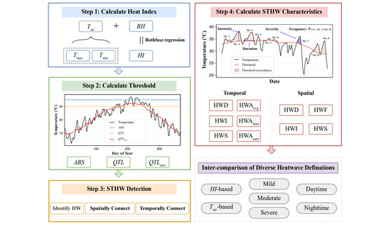
:A heatwave (HW) is a spatiotemporally contiguous event that is spatially widespread and lasts many days. HWs impose severe impacts on many aspects of society and terrestrial ecosystems. Here, we systematically investigate the influence of the selected threshold method (the absolute threshold method (), quantile-based method (), and moving quantile-based method ()) and selected variables (heat index (), air temperature ()) on the change patterns of spatiotemporally contiguous heatwave (STHW) characteristics over China from 1961–2017. Moreover, we discuss the different STHW change patterns among different HW severities (mild, moderate, and severe) and types (daytime and nighttime). The results show that (1) all threshold methods show a consistent phenomenon in most regions of China: STHWs have become longer-lasting (6.42%, 66.25%, and 148.58% HW days () increases were found from 1991–2017 compared to 1961–1990 corresponding to , , and , respectively, as below), more severe (14.83%, 89.17%, and 158.92% increases in HW severity () increases), and more spatially widespread (14.92%, 134%, and 245.83% increases in the summed HW area ()). However, the HW frequency () of moderate STHWs in some regions decreased as mild and moderate STHWs became extreme; (2) for threshold methods that do not consider seasonal variations (i.e., and ), the spatial exceedance continuity was relatively weak, thus resulting in underestimated STHW characteristics increase rates; (3) for different variables defining STHWs, the relative changing ratio of the -based STHW was approximately 20% higher than that of the -based STHW for all STHW characteristics, under the threshold; (4) for different STHW types, the nighttime STHW was approximately 60% faster than the daytime STHW increase considering the threshold and approximately 120% faster for the method. This study provides a systematic investigation of different STHW definition methods and will benefit future STHW research.
1. Introduction
Heatwaves (HWs) severely impact many aspects of society and terrestrial ecosystems [1,2,3,4]. For example, HWs can directly cause organ damage and a range of cardiovascular diseases (e.g., myocardial infarction and heat exhaustion) and indirectly increase the risk of spreading viruses [5,6,7,8]. Additionally, HWs can reduce food and water supplies and increase potential conflicts, such as the mortality caused by HW and other environmental and social problems. For example, the 2012 extreme HW in the United States led to a maize production decrease of 13% compared to the 2011 level [9]; the 2013 extreme HW in southern China led to a net reduction of 101.54 Tg C in regional carbon sequestration in two months and the most extensive crop failures since 1960 [10].
In the past few decades, many researchers have devoted themselves to revealing the change patterns of HWs in the warming climate. However, different researchers have used different methods to define HW events. It is generally accepted that an HW is an episode when the temperature variable exceeds a certain threshold. However, when selecting a more particular definition, divergences arise regarding which threshold method and temperature variable to use [11,12,13]. For the threshold, there are three prevalent methods: the absolute threshold method (), the quantile-based method (), and the moving quantile-based method () [12,13]. For example, a HW is recognized by the Royal Netherlands Meteorological Institute as a period when the daily maximum temperature is greater than 25 °C for more than five consecutive days. Following the World Meteorological Organization’s (WMO) suggestions, HWs occur when the daily maximum temperature surpasses the average maximum temperature by 5 °C for five consecutive days. In China, HWs are defined as events exceeding 35 °C and lasting at least three consecutive days, according to the Chinese National Meteorological Administration. These commonly used threshold features are summarized in Table 1. Regarding the temperature variable, some studies have used air temperature () [14,15,16,17]. However, many studies have argued that the heat index () is more relevant to human-perceived temperature [18] and is thus more suitable to define HWs [19,20,21,22]. Although some significant progress has been made, the impacts of variable selection on the spatiotemporal change pattern of HWs are not well understood.
On the other hand, HW is a kind of spatiotemporally continuous event that are spatially widespread and last many days, transferring from one region to another, and merging or splitting over time during their development and diminution. However, most previous studies have ignored these HW characteristics and studied HWs simply at the grid or site scale. With advances in the spatiotemporal clustering technique [23,24], it has become feasible to track spatiotemporally contiguous heatwaves (STHWs) and study their change patterns on the 3-D event scale [12,25,26,27]. However, HW studies performed at this 3-D event scale are much fewer than those performed at the grid and site scales. Consequently, the problem of the effects of the variable and threshold method selection on the STHW changing pattern is increasingly prominent.
Therefore, in this study, we mainly attempt to illustrate the influence of threshold method selection (the absolute threshold method (), quantile-based method (), and moving quantile-based method ()), variable selection (heat index (), air temperature ()) on the change patterns of spatiotemporally contiguous heatwaves (STHWs) characteristics over China from 1961 to 2017. In addition, we provide an in-depth discussion on the drivers of differences in the intercomparison of HW definitions.
2. Data and Methods
2.1. Data
The daily maximum air temperature (), minimum air temperature (), and relative humidity () are used in this study. The and data are derived from CN05.1 [28] at a spatial resolution of 0.25° covering 1961–2021 period. The CN05.1 dataset is interpolated from 2416 stations in mainland China with strict quality control [28]. Previous studies have revealed that unhomogenized could lead to a fake decreasing trend of in South China [29,30]. To avoid this problem, we used ChinaRHv1.0, a homogenized dataset containing site observations from 746 stations on the Chinese mainland from 1960–2017 [30]. We interpolated ChinaRHv1.0 into 0.25° by the same method as that applied to CN05.1 [28], where the thin-plate spline method was proposed for the climatology and the angular distance weighting method was proposed for the anomaly. The interpolated climatology-plus-anomaly result forms the final gridded dataset. Limited by the coverage period, we analyze STHW only from 1961 to 2017.
2.2. Heat Index
In previous research, either or was used to evaluate HW. However, there is no definite conclusion as to which of these is more suitable. In this paper, both variables are used for comparison. (in °C), also known as the apparent temperature, is more correlated with the human-perceived temperature [31,32] and is calculated through Rothfusz regression [21,22,33]:
2.3. HW Thresholds
If the temperature of a grid cell exceeds its corresponding threshold, we consider that a HW has occurred here. The determination of thresholds consists of two main components: quantiles and calculation methods. The detailed classification is described below:
The quantile can also refer to the HW severity levels depending on its magnitude: (1) 90th (i.e., mild level), (2) 95th (i.e., moderate level), and (3) 99th (i.e., severe level). When the quantile is greater than the 99th percentile, only a few HW events are identified. Such a small sample size would considerably impair the reliability of the estimated trends. This could lead to an uncertainty factor that is too large to reflect the variation trend patterns of most HW events.
Regarding the calculation methods, three methods are selected, including (1) , (2) , and (3) .
- (1)
- For the method, all grid cells share the same threshold and eastern China (longitude ≥ 105 °E) is used to compute the threshold. First, the regional area-weighted average of or is calculated at each time step. The thresholds are determined in accordance with certain percentiles (i.e., 90th, 95th and 99th corresponding to mild, moderate and severe HWs, respectively) during the 1961–1990 reference period from the time series.
- (2)
- For the method, each grid has a unique threshold. For each grid, the threshold is calculated as a certain percentile during the 1961–1990 reference period.
- (3)
- For the method, the threshold varies among each day of the year () from 1 to 366 in the Julian calendar. For each grid, a 15-day moving window (i.e., 7 days prior and posterior to the corresponding calendar day sampled from each year) for each is used to create a subset, and a specific quantile calculated during the 1961–1990 reference period is used as the threshold corresponding to the center date. For instance, all 1 January to 15 January data from 1961–1990 are selected, and the threshold for 8 January is the quantile of these 450 days. Due to the dramatic temperature changes that have occurred in China since the 1990s, it is appropriate to take 1961–1990 as the reference period for a historical comparison and climate change monitoring; this application is also recommended by the WMO [34].
2.4. STHW Detection
In spatiotemporal detecting, the HW spatial-state array (i.e., whether the temperature is greater than or equal to the threshold) is used as the input, and temporally and spatially contiguous grid cells are connected to the same STHW event. This idea has been applied in drought studies previously [35]. The 3-D connectivity algorithm is relatively common but is rarely used in HW identification tasks. It is often used for lesion tracking in medical and 3D image denoising, and similar functions can be found in the Python package scikit-image, MATLAB tool , R package , and so on [36].
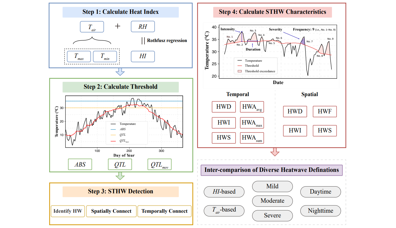
Here, we rewrite the spatiotemporal clustering algorithm of Samaniego [24] to detect STHWs. Compared to the original version, ours has an excellent computing efficiency (e.g., 30~50 times faster, thanks to the speed of the Julia language), low memory consumption (e.g., uses the disjoint-set data algorithm) and can also connect contiguous temporally related HW events (e.g., all merging, splitting, expanding, and receding HW events associated with a specific event) into the same STHW event. Figure 1 briefly illustrates the main steps of this process, and the computational implementations are as follows:
- (1)
- The original data are converted to the HW spatial-state array. Initially, the original data have three dimensions (i.e., longitude × latitude × time). For each voxel, if the value is greater than the corresponding threshold, it is marked as “True” and considered as HW grid; otherwise, it is marked as “False”. The threshold is calculated as described in Section 2.3. Therefore, the data are converted to an HW spatial-state array that is stored in a “True/False” Boolean format.
- (2)
- Spatially adjacent HW grids are connected to spatial HW events. In this step, the HW state array is cyclically traversed moment-by-moment in a top-to-bottom, left-to-right order to search for spatially adjacent voxels in each time layer. If an HW grid is detected, it is given a unique . After that, according to the 4-connected neighborhood principle (i.e., two adjoining cells are part of the same object if they are both on and are connected along the horizontal or vertical direction), all recursively searched edge-adjacent HW grids are given the same . Here, a merged spatial HW event with a grid number less than is eliminated, because a small isolated HW event is usually unable to develop into a regional or impactful STHW event; is set to 16.
- (3)
- The spatial HW events are connected to spatiotemporally contiguous HW events. If there are at least grids at the same location in the preceding and following time steps from two spatial HW events, the events are merged into one STHW event and given a new (, where is the of the previous spatial HW event). Here, is set to correspond to . Because HW events usually have a small scale when appearing and dying, this threshold can be set to better distinguish different STHW events from the onset and demise. Finally, the values are stored in three dimensions as original data (i.e., longitude × latitude × time). Due to the thresholds, the identified STHW can ensure that the spatial coverage is not too small and lasts at least 2 days.
Figure 1.
The proposed method for detecting STHWs. (a) The identified STHW events from 28 June to 1 July 2017, in China; the features of merging and splitting events are labeled in the third step. (b) Explanation of the STHW clustering process, including three steps: (1) identifying HWs; (2) spatially connecting HWs; and (3) temporally connecting HWs.

Based on the selection of the temperature and data variables, the STHW types are separated into two groups: (1) daytime STHWs identified by the daily maximum temperature and (2) nighttime STHWs identified by the daily minimum temperature. Similarly, -based STHWs and -based STHWs are identified by the air temperature and heat index, respectively.
To date, these diverse HW definitions can be derived from different threshold calculation methods (, and ), severity levels (mild, moderate and severe), types (daytime and nighttime), and data variables ( and ). The rest of this study is based on the use of control variable methods to compare these definitions.
2.5. STHW Characteristics
To evaluate STHW, STHW characteristics are defined separately at temporal and spatial scales. The temporal characteristics are all counted at the event scale (Table 2). Here, we focus only on the most impactful STHW event of the year, corresponding to the largest HW severity () each year. Because the number of small STHW events is much larger than that of typical HW events, tracking only the annual largest STHW event can prevent a large number of small events from offsetting the real temporal variants. Here, HW days () expresses the duration of STHW events, HW intensity () and are used to describe the intensity and cumulative intensity, respectively, and HW area () is the occurrence area, which is further divided into three aspects: the mean, maximum, and total area.
In contrast to our focus only on the severest HW event temporally, all HW events that occur over the year are counted in the spatial analysis (Table 3). This is because the spatial HW characteristics should reflect the overall spatial HW distribution, while the largest annual event cannot mask the entire country. Here, is calculated based on the number of days the HW occurs; HW frequency () is added to express the number of HW events; and and are still calculated by obtaining the anomaly between the temperature and threshold.
3. Results
3.1. STHW Characteristics of Different Threshold Methods
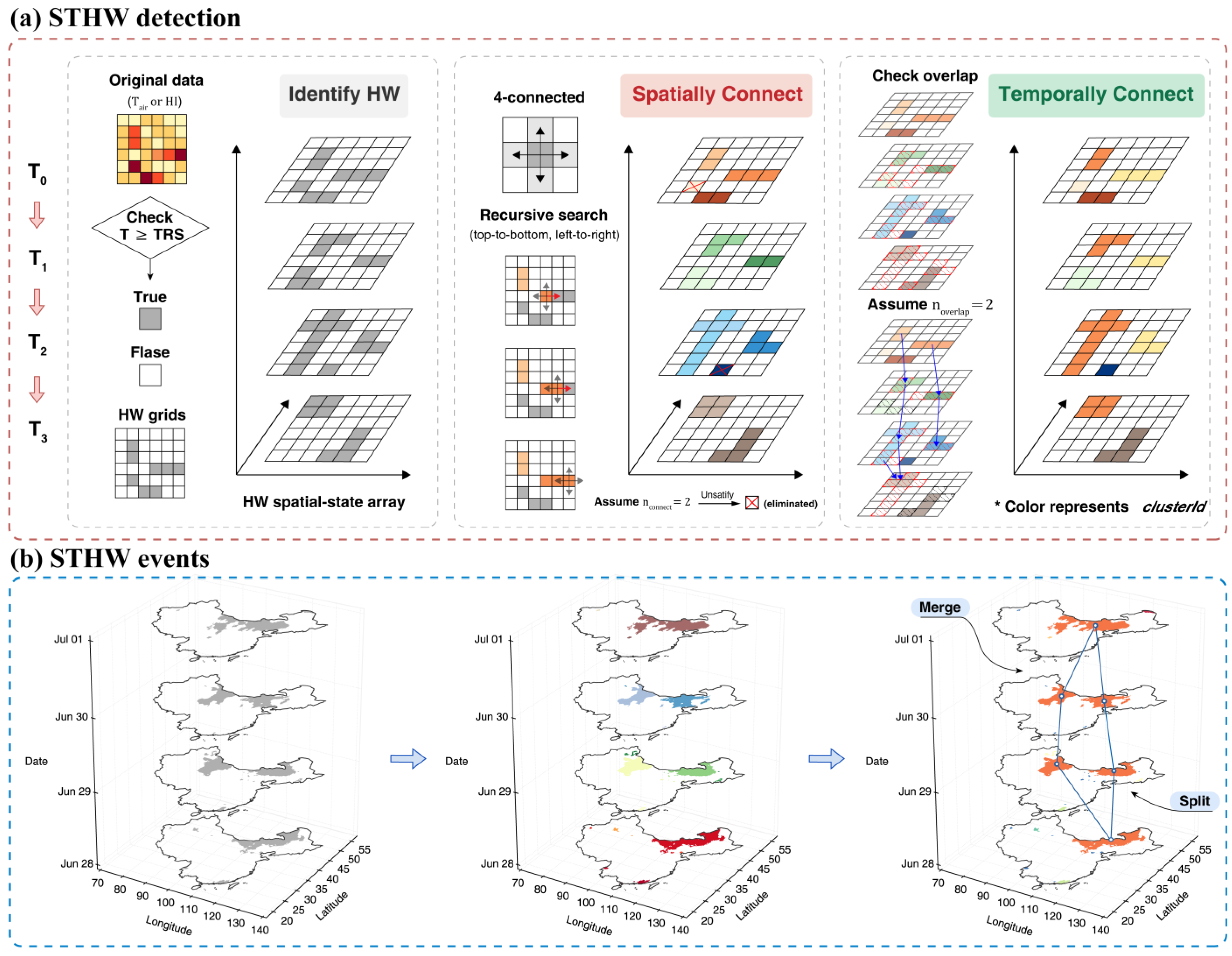
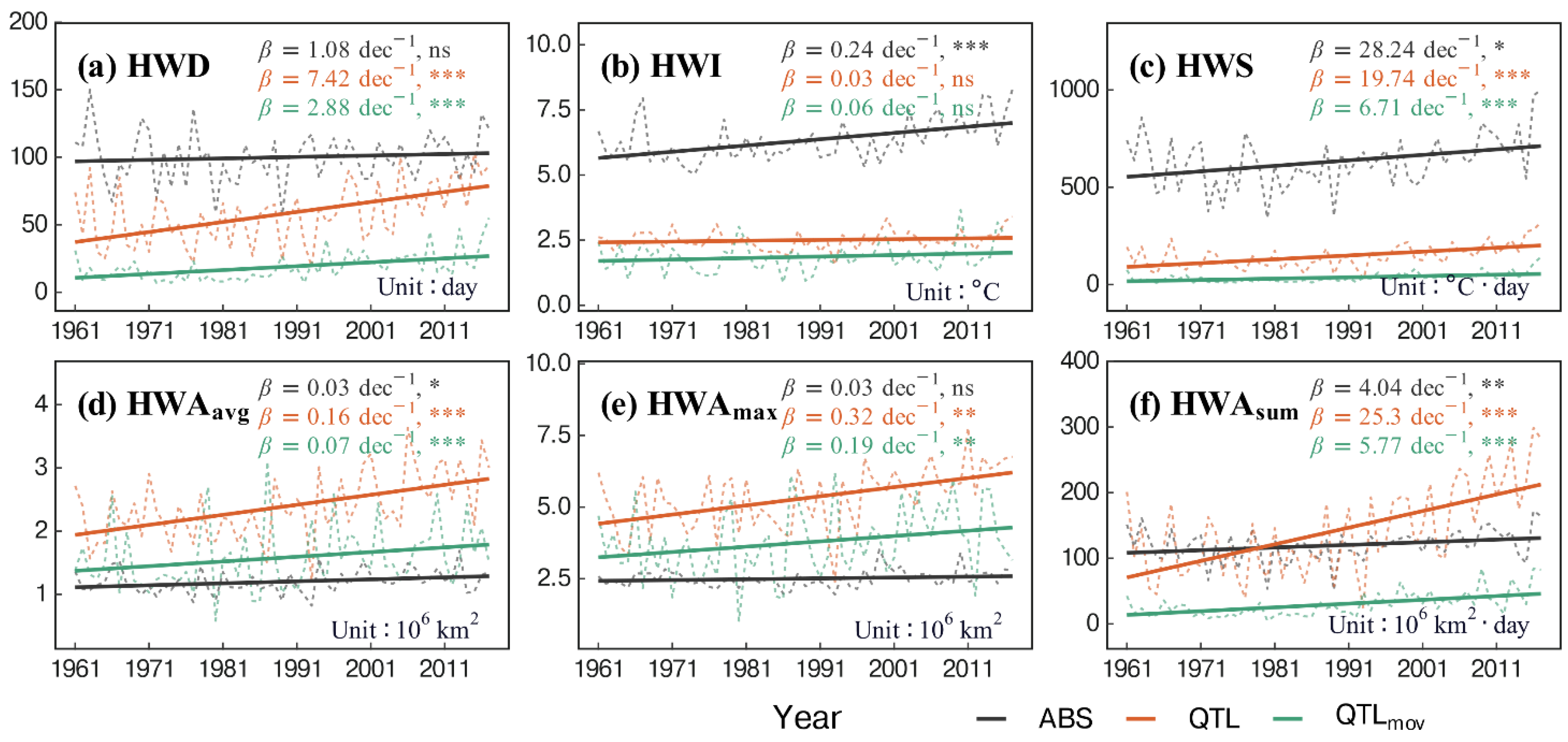
Figure 2 shows the annual variations in the characteristics of the most severe STHW events that occurred in China from 1961–2017, defined by three different threshold methods: , and . The magnitudes of the STHW characteristics vary substantially among different threshold methods. For , , and , the magnitudes obtained with the method are significantly larger than those obtained with and , with the rank of > > . The mean values obtained with are 100.00 days, 6.33 °C, and 632.71 °C∙days for , , and , respectively. In comparison, these mean values are only 58.00 days, 2.50 °C, and 145.82 °C·days, respectively, for and 18.75 days, 1.86 °C and 35.88 °C∙days, respectively, for . For and , the situation is reversed. The rank becomes > > , and the mean values of are 2.38 × 10⁶ km2, 1.58 × 10⁶ km2 and 1.20 × 10⁶ km2, respectively, while the mean values are 5.31 × 10⁶ km2, 3.77 × 10⁶ km2 and 2.51 × 10⁶ km2, respectively, for those three threshold methods.
Regarding the trends, for , the threshold exhibits an increasing trend of 7.42 days/decade, much higher than the trends obtained using the other methods (1.08 days/decade and 2.88 days/decade) but not significantly so. and exhibit similar results. The threshold always indicates the highest slope, reaching 0.24 °C/decade and 28.24 °C·day/decade. However, for , only the threshold shows significance, while all methods show significance for . For all area-related characteristics, the threshold identifies the highest increasing rate. Especially for , the threshold shows an amazing trend of 25.3 × 10⁶ km2/decade, approximately 4–5 times higher than those obtained with the other methods. In comparison, the threshold has the lowest increasing rates of 0.03 km2/decade, 0.03 km2/decade, and 4.04 km2/decade corresponding to , , and , respectively.
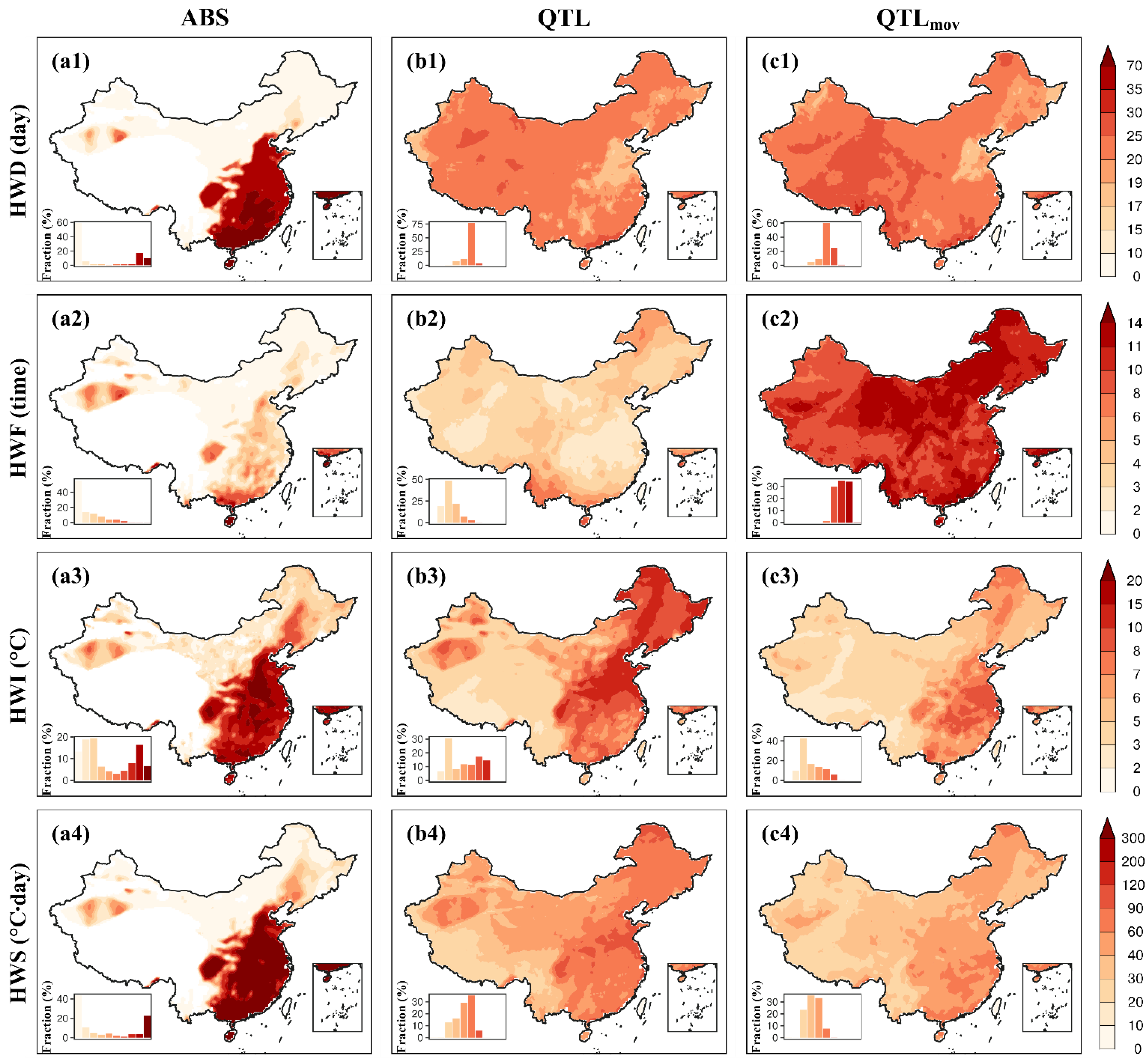
Regarding the spatial magnitude (Figure 3), except for , the magnitudes obtained with and are similar for all STHW characteristics. Because the method focuses only on the highest temperature period, while considers all periods in a year, detects more STHWs than , resulting in a higher (Figure 3b2,b3). Using the method, the derived spatial distribution of the multiannual average STHW characteristics is substantially different from those obtained with and . Most STHWs are detected in the North China Plain and South China, while no STHWs are detected on the Tibetan Plateau because of the low climatological temperatures there.
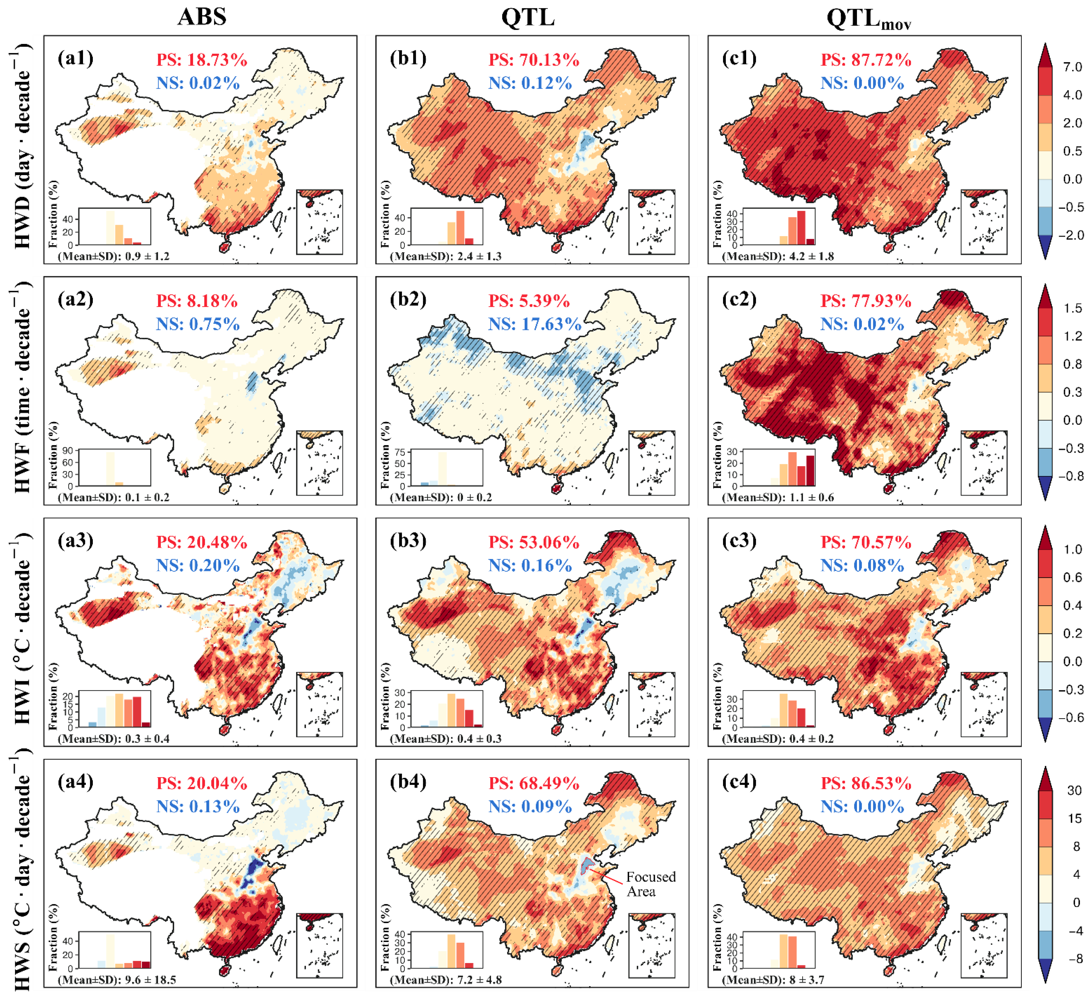
Regarding the spatial trend, the three analyzed methods show consistently increasing trends for all STHW spatial characteristics except (Figure 4). The STHWs become longer in duration, more widespread in impact, and more intense in intensity and severity. Regarding , , and , the ranking of the increase rates is > > . For , , and , there is a prevalent and consistent increasing trend among , and . However, for , the increasing trend is not significant in most regions of China (Figure 4a2,b2) and even becomes negative in North China (Figure 4b2). This is mainly because mild and moderate STHWs gradually turn into severe STHWs under the warming climate conditions. The frequency of mild and moderate STHWs decreases, while that of severe STHWs increased (Figures S1 and S2). Additionally, for , , and , noticeable decreasing trends arise in the middle of the North China Plain and across large parts of Northeast China.
3.2. HI-Based and -Based STHWs
Many researchers utilize rather than to measure HWs, though this may produce errors when attempting to accurately reflect HWs’ impacts on humankind. Moreover, the results may differ to a relatively great extent due to the addition of relative humidity. Hence, we compare the difference between -based and -based STHWs.
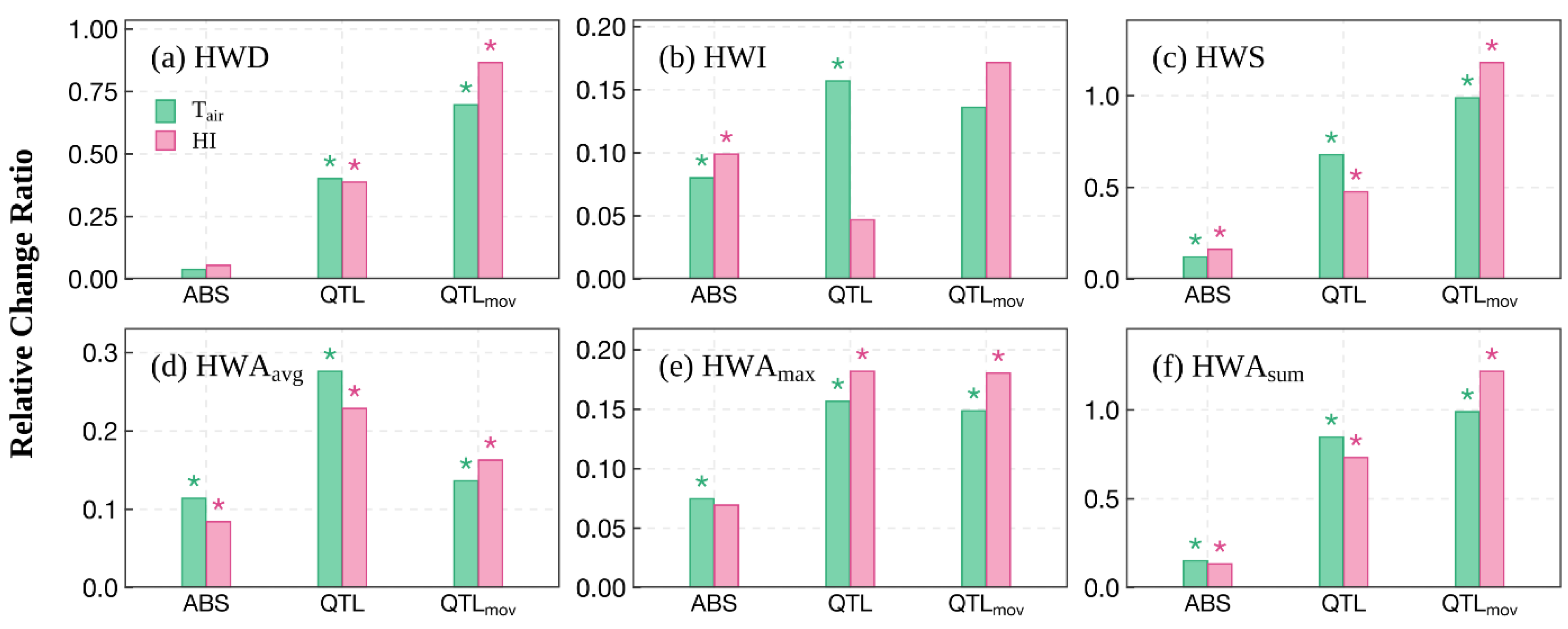
Figure 5 presents the difference between the -based and -based moderate daytime STHWs from the perspective of the relative change ratio between the present period of 1991–2017 and the historical period of 1961–1990 in China. Regarding the threshold, the relative change ratio of the -based STHW is approximately 20% higher than that of the -based STHW for all STHW characteristics (Figure 5). For the three threshold methods, the differences in the relative change ratio between the -based and -based STHWs are extremely small, especially when using the threshold. Moreover, regarding the method, the result is even reversed; the relative change ratio of the -based STHW is lower than that of the -based STHW. For threshold methods that do not consider any seasonal variation (i.e., and ), the spatial continuity of the -based exceedance is weaker than that of the -based exceedance, thus contributing to the weak and reversed phenomena observed when using the and threshold methods.
3.3. STHWs with Different Severity Levels
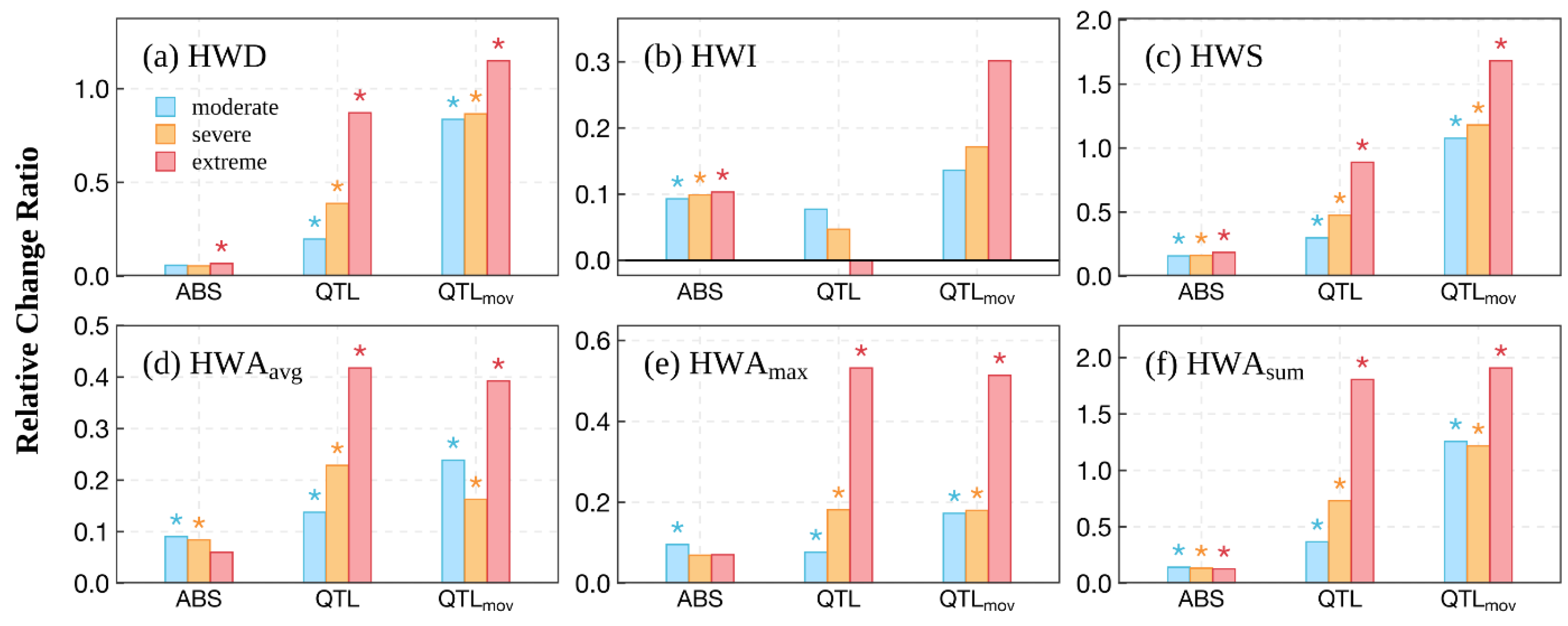
Figure 6 shows the relative change ratios of STHW characteristics between the present and historical periods under different HW severity levels in China. As the severity level rises, most characteristics show increased growth trends together with significance. Specifically, under extreme severity levels, the values obtained with the and threshold methods reach 0.51 and 0.53, respectively, with increases of nearly 50% and at least threefold compared to the mild and moderate levels (0.17 and 0.18 for the threshold, 0.08 and 0.18 for the threshold). Generally, compared to mild STHWs, the average relative change ratios of moderate and severe STHWs among different STHW characteristics are approximately 1.2 and 2.4 times higher, respectively, indicating that extreme STHWs increase much faster than mild and moderate STHWs; this finding is consistent with the results of previous HW studies performed at the grid scale [22]. However, when using the threshold method, these values are approximately 0.87 and 0.93 times smaller than those of mild STHWs, further confirming that the spatial continuity of the results obtained using the threshold method is weak and may be unsuitable for STHW detection. Because most nonsignificant trends occur in the results, we mainly focus on comparing the other five indexes. Among those five indexes, the relative changing ratio of is the highest, while that of ranks second, indicating that the impacted spatial areas of extreme STHWs increase much faster than their duration, intensity, and severity.
Figure 3.
Spatial distributions of the multiannual average daytime, moderate, -based STHW spatial characteristics from 1961–2017: the combination results of using (a) , (b) and (c) method and (1) , (2) , (3) and (4) characteristics. The frequency distribution is shown in the lower-left corner of each subplot.

Figure 4.
Spatial distribution of the annual trend of -based, moderate, daytime STHW characteristics from 1961–2017: the combination results of using (a) , (b) and (c) method and (1) , (2) , (3) and (4) characteristics. The filled color represents the value of Sen’s slope. The hatches denote trends that are significant at the 0.05 level. For each subplot, the percentages of positively significant (PS) and negatively significant (NS) trends are shown in the top-center, and a histogram of trends is plotted in the lower-left corner. The frequency distribution is shown in the lower-left corner of each subplot. In b4, the highlighted area is the focus area used to explain the negative trends in Section 4.1.

Figure 5.
The change ratios of temporal STHW characteristics between the present period of 1991–2017 and the historical period of 1961–1990: for (a) , (b) , (c) , (d) , (e) and (f) . Daytime, severe STHWs are used here. The change ratio equals , where and are the mean values of the considered STHW characteristics during the historical and present periods, respectively. The “*” symbol denotes that the Sen’s slopes of the STHW characteristics from 1961–2017 are significant at the 0.05 level.

Figure 6.
Same as Figure 5, but comparing different HW severity levels. The -based, daytime STHW results are used here.
Figure 6.
Same as Figure 5, but comparing different HW severity levels. The -based, daytime STHW results are used here.

3.4. Daytime and Nighttime STHWs
Figure 7 compares the differences in the relative change ratios of STHW characteristics between daytime and nighttime STHWs. Surprisingly, daytime STHWs show higher ratios only for but lower ratios for , , , , and . For instance, for the values identified by the threshold, the ratios corresponding to daytime and nighttime STHWs are 0.10 and 0.07, respectively. For the threshold method, daytime STHWs possess at least twofold higher (1.84 and 0.87), (0.36 and 0.16), (0.56 and 0.18), and (3.11 and 1.22) values than nighttime STHWs. Overall, the results show that the average increase in nighttime STHWs is approximately 60% faster than that of daytime STHWs when using the threshold, and approximately 120% faster when using the method.
4. Discussion
4.1. Explanation of Negative STHW Characteristic Trends in North China and Northeast China
Although prevalent increasing trends in spatial STHW characteristics (e.g., , , and ) are observed in most regions of China, significant decreasing trends are presented in parts of North China and Northeast China (Figure 4). Taking one representative region, North China, as an example, we further illustrate the underlying reasons for these decreasing trends (Figure 8 and Figure 9).
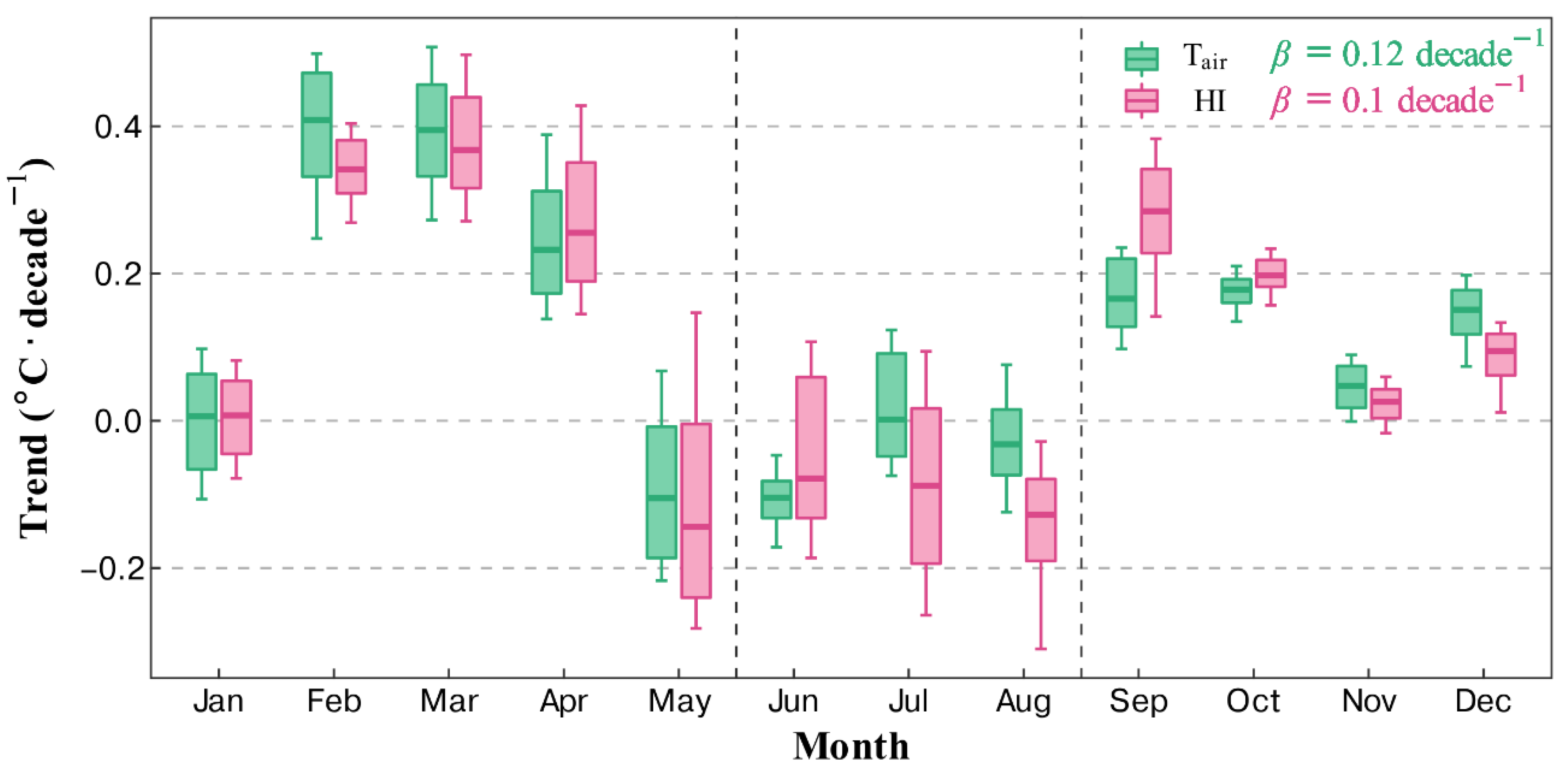
We found that negative STHW trends can be attributed to the following two aspects: (1) On the one hand, temperature warming is spatially asymmetric. Although increasing temperatures are prevalent in most regions of the globe [37], some regions are experiencing the inverse trend, with significant decreasing temperature trends. North China is one of these cases [38,39]. Undoubtedly, the decreasing local temperatures contribute to the decreasing STHW characteristics at the spatial level. (2) On the other hand, temperature warming is asymmetric over time. As shown in Figure 9, strong increasing temperature trends are observed in spring and autumn; a weak increasing trend is observed in winter; and reverse decreasing trends are observed in summer and at the end of spring. We also found that decreasing primarily contributes to the decreasing in summer (Figure 8) and, hence, to the asymmetric warming observed among different methods. This phenomenon directly leads to the decreasing trends of threshold-based STHW characteristics, as the threshold method mainly focuses on the hottest period each year (namely, summer), when significant decreasing trends occur. Moreover, regarding the threshold-based STHWs, this phenomenon weakens the increasing STHW trends. However, whether the trend direction becomes negative depends on the increasing STHW magnitudes in other seasons, as focuses on anomalies throughout the whole year.
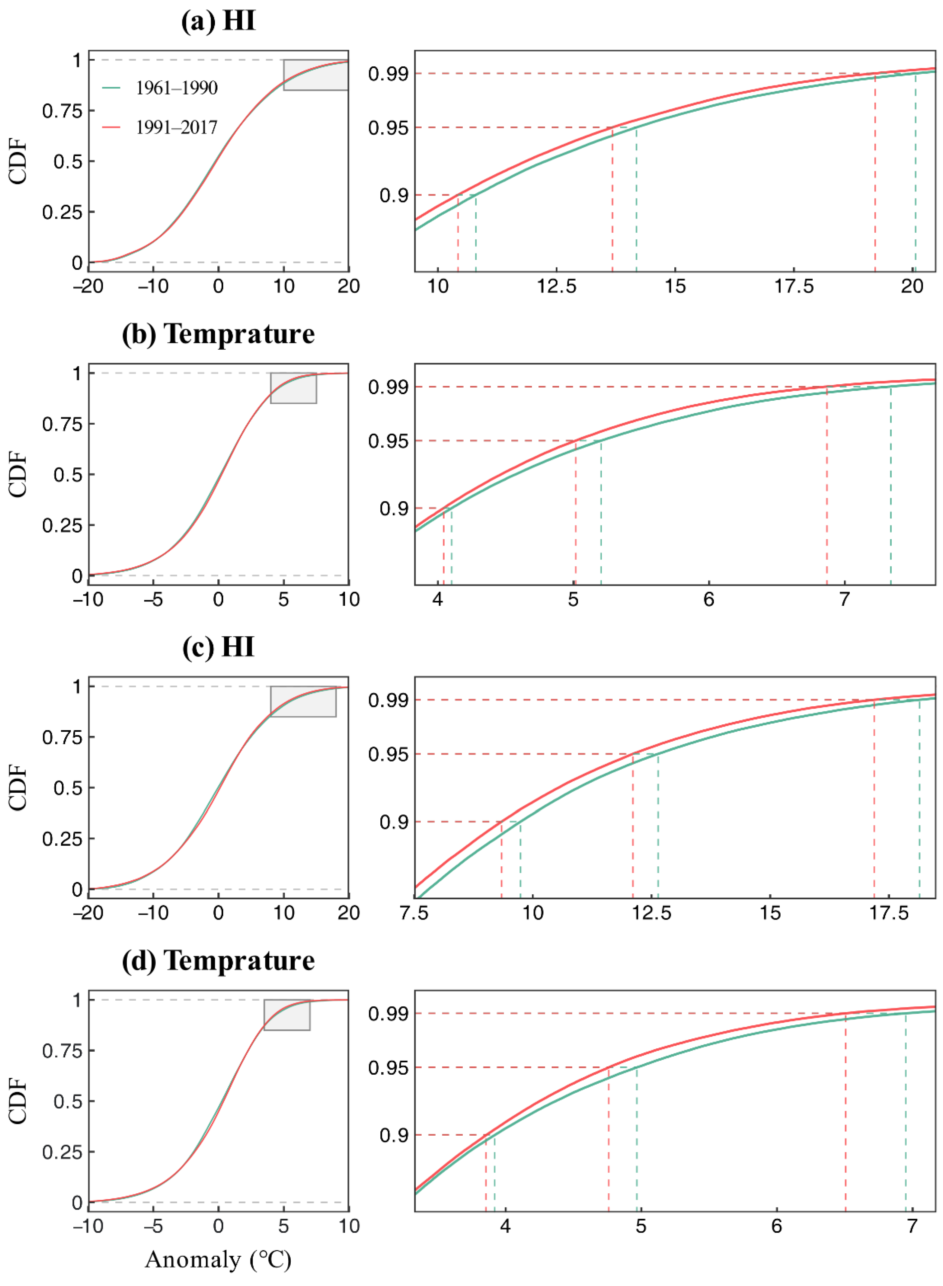
Figure 9 further investigates the offsetting effect of summertime cooling and warming in other seasons regarding the -based STHW results in North China. The figure shows that although the annual averaged and have positive trends, the 90%, 95% and 99% quantiles of their -based anomalies in the current period from 1991–2017 apparently decrease compared to those in the historical period from 1961–1990 (Figure 9). This indicates that summertime cooling has a stronger impact on the negative STHW trends in the spatial component than warming in other seasons in North China and explains the negative STHW characteristics trends derived in North China.
4.2. Possible Reasons for the STHW Characteristic Differences among Different STHW Definitions
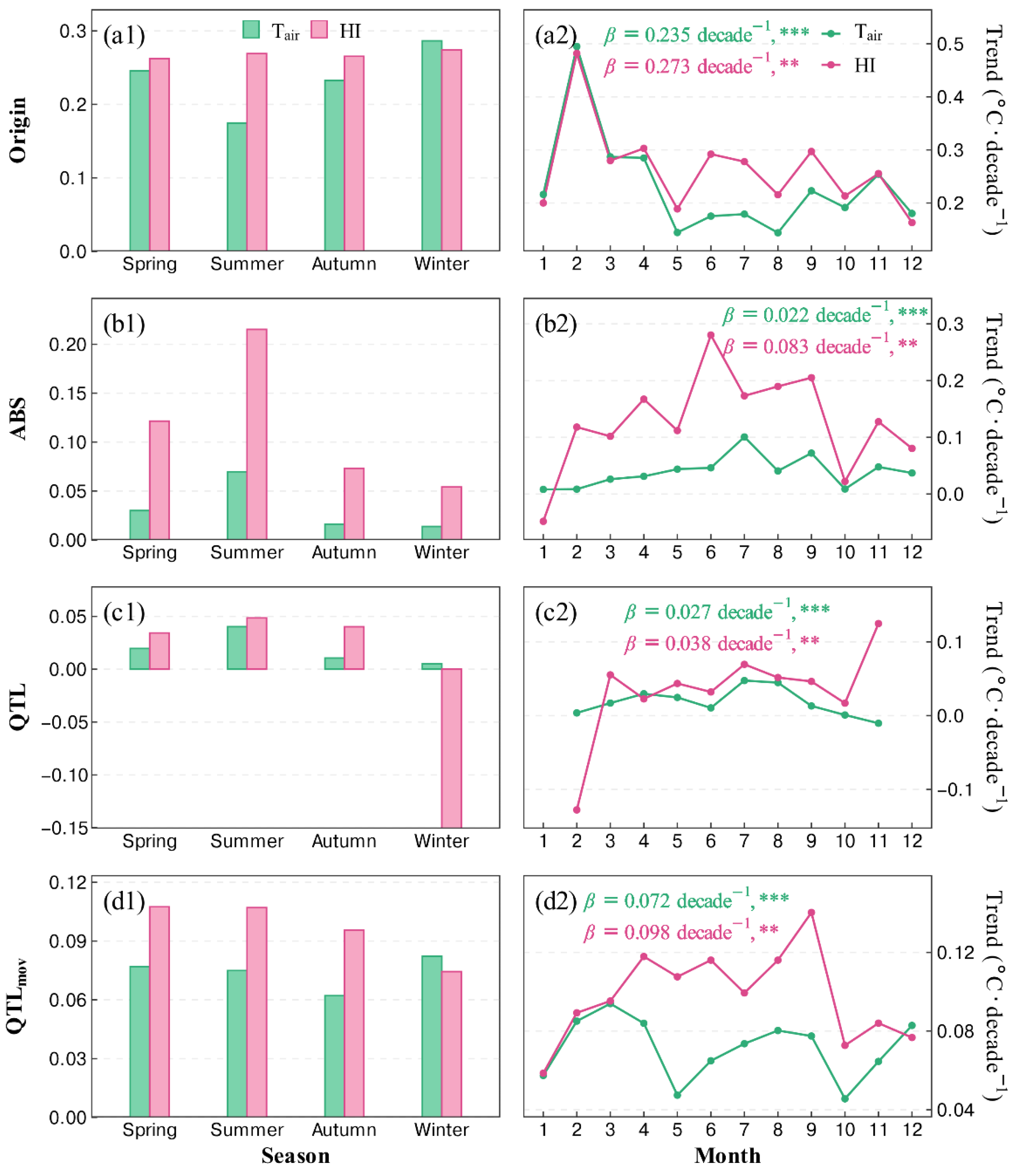
There is evidence that increases faster than regardless of the area-weighted original value or area-weighted anomaly (Figure 10a1–d1). This result is consistent with previous findings that the joint impact of reduced and increased temperatures leads to more unprecedented HWs [3,13,36]. However, only for the threshold do the -based STHW characteristics always present higher ratios than the -based characteristics (Figure 5). This result implies that the threshold is more suitable for STHW detection. For threshold methods that do not consider seasonal variations (i.e., and ), the spatial continuity of the exceedance is relatively weak, thus resulting in the increase rates of STHW characteristics being underestimated.
Regarding different HW severity levels, the averaged relative change ratios of moderate and severe STHWs among different STHW characteristics are approximately 1.2 and 2.4 times higher than those of the mild STHW for the and threshold methods, respectively, implying that extreme STHWs will increase much faster. Due to relatively the low numbers of STHW events identified as the severity level increases. The occurrence of fewer events will cause the extreme values to be more prominent, and more STHW events may “average” the results, resulting in relatively low change ratios.
Regarding daytime and nighttime STHWs, the increase in nighttime STHWs is approximately 60% faster than that in daytime STHWs using the threshold and approximately 120% faster using the method. In addition, the latter method usually results in a higher change ratio than the former. This finding is consistent with previous studies [17,40,41] and is mainly the result of intensified heating at nighttime compared to daytime (0.46 °C∙decade−1 at nighttime and 0.42 °C∙decade−1 at daytime) [17,42,43], further leading to an increasing tendency for nighttime HWs to replace the previously dominating independent daytime events [17]. As a further explanation, Luo [44] revealed that increased cloud cover can reduce the solar radiation received by the land surface, thus potentially increasing the downward longwave radiation emitted by the atmosphere and clouds at the surface at night and leading to reduced cooling of longwave radiation and increased nighttime temperatures. This may be the root cause of such rapid increases in nighttime HWs.
4.3. Significance and Limitations
Recently, Luo [25] proposed a 3D perspective to analyze the spatiotemporal patterns of HWs. In his result, the characteristic trends are 1.14 days/decade for the HW lifetime, 0.04 °C/decade for the HW intensity, 0.18 × 10⁶ km2/decade for the maximum area and 1.30 × 10⁶ km2/decade for the total area, while the corresponding metrics obtained in our study are 2.88 days/decade for , 0.06 °C/decade for , 0.19 × 10⁶ km2/decade for and 5.77 × 10⁶ km2/decade for . Compared to his approach, we focused on the most impactful STHW events regarding the temporal characteristics, resulting in relatively high increasing growth in and . Apart from these indexes, our results show a high degree of consistency. Despite the divergences among the analyzed methods, both results showed significantly positive trends, demonstrating the robustness of our results.
The study offers some important insights, outlined as follows:
- (1)
- An improved algorithm is used to detect STHWs. Instead of simply merging all temporally and spatially adjacent HW grids into a single STHW event, we set two thresholds: and . Compared to the ordinary 3D connection algorithm, this method considers the merging and splitting behaviors of STHW events during their development and diminution.
- (2)
- Past articles rarely used spatiotemporal clustering algorithms to compare the spatiotemporal patterns under different HW definitions. The majority of investigations of spatial or temporal variations focused only on the grid scale and ignored joint spatial and temporal evolution pattern. In addition, -based HWs are closely relevant to human perception, and while most past studies used either or , the difference among these variables remains largely unexplored. In our study, we compare these HW definitions as comprehensively as possible.
Due to practical constraints, this paper cannot provide a comprehensive review of the following considerations:
- (1)
- The data selection method may influence the results, especially for . According to our early study, using unhomogenized data can produce entirely different results. To ensure the objectivity of the results, we replaced the original with a homogenized . However, the differences introduced by different homogenization methods were not assessed. It is thus better to use multiple datasets to demonstrate the robustness of the results. In addition, the selection of temperature data may produce differences, as expressed in the trend magnitudes and the different distributions of spatial characteristics, but not to the same extent as the selection.
- (2)
- Different selections of the and thresholds were not investigated herein. Comparing the similarity of the results derived with different thresholds may enhance the robustness of our result.
Overall, our study can provide a more comprehensive understanding of the change patterns of STHW events in China and help researchers select a suitable HW definition in China in future research. However, the influence of the chosen data and and values remains unknown in this work, and this will be an important issue in future research.
5. Conclusions
In this study, we used a modern spatiotemporal clustering algorithm to detect spatiotemporally contiguous heatwaves (STHWs) from a 3-D perspective in China from 1961–2017. We systematically investigated the influence of various threshold methods (, , and ), variables ( and ), severity levels (mild, moderate, and severe), and time (daytime and nighttime) selections on the STHW change characteristics. The results suggest the following:
- (1)
- Although the trends’ magnitudes were divergent, all threshold methods showed a consistent phenomenon in most regions of China: STHWs have become longer-lasting, more severe, and have impacted larger areas spatially. However, the increasing trends identified in most cases are insignificant. Moreover, the of the moderate STHWs has decreased mainly because the transfer of mild and moderate STHWs to extreme STHWs decreased the frequency of the former events. In small parts of central-eastern and northeast China, some negative STHW trends were observed due to asymmetric warming in these areas, i.e., these regions experience negative trends in summer but positive trends in other seasons. For threshold methods that do not consider any seasonal variation (i.e., and ), the spatial continuity of the exceedance is relatively weak, resulting in the increase rates of STHW characteristics being underestimated. In addition, the method uses eastern China to calculate the threshold, and it is difficult to identify HWs for the lower-elevation areas in western China (e.g., the Tibetan Plateau). In comparison, performs much better and is more suitable for use across China.
- (2)
- Regarding -based and -based STHWs, when using the threshold, the relative change ratios of all -based STHW characteristics are approximately 20% higher than the -based STHW characteristics, suggesting that the contribution of to HW variability is visible and causes human-perceived HWs to increase rapidly, as hot temperatures are even more unbearable as the presence of humidity in the environment reduces the ability of the human body to cool itself. Therefore, -based STHW should be priorly used. alone without considering may underestimate the increasing STHW magnitudes. However, this phenomenon is weak when considering the threshold and is even reversed when using the method due to the weak spatial continuity of these two methods.
- (3)
- Regarding different HW severity levels, the averaged relative change ratios of moderate and severe STHWs among different STHW characteristics are approximately 1.2 and 2.4 times higher than those of mild STHWs when using and threshold methods, respectively, implying that extreme STHWs will increase much faster than mild or moderate STHWs; this finding is inextricably related to climate warming. Therefore, this phenomenon requires preparation and mitigation programs to avoid or mitigate the effects of the rapid growth of extreme weather events.
- (4)
- Regarding daytime and nighttime STHWs, the increase in nighttime STHWs is approximately 60% faster than that of daytime STHWs when applying the threshold and approximately 120% faster when applying the method. Increasing nighttime exposures may increase the risk of heat-related illnesses.
Our study provides a systematic investigation of different STHW definition methods and will benefit HW studies in the future.
Supplementary Materials
The following supporting information can be downloaded at: https://www.mdpi.com/article/10.3390/rs14164082/s1 and https://zenodo.org/record/7012026. Figure S1. Same as Figure 3, but the -based, daytime, mild STHW results are used here. Figure S2. Same as Figure 3, but the -based, daytime, severe STHW results are used here.
Author Contributions
Conceptualization, D.K.; software, H.S. and D.K.; data curation, L.X.; writing—original draft preparation, H.S. and D.K.; writing—review and editing, H.S., D.K., X.G. and J.L.; visualization, H.S. All authors have read and agreed to the published version of the manuscript.
Funding
This study was supported by the Natural Science Foundation of Hubei Province (Grant 2021CFB198), the National Natural Science Foundation of China (Grants 4210011820, 41901041, and 42001042), the Fundamental Research Funds for the Central Universities, China University of Geosciences (Wuhan) (Grant CUG2106107).
Data Availability Statement
The CN05.1 dataset can be available at http://ccrc.iap.ac.cn/resource/detail?id=228 (accessed on 28 March 2022). The homogenized data is available at https://www.scidb.cn/en/detail?dataSetId=633694461334913025 (accessed on 5 April 2022).
Acknowledgments
The authors thank Wu, J. for providing CN05.1 and Li, Z. for providing homogenized data.
Conflicts of Interest
The authors declare no conflict of interest.
Abbreviations
The following abbreviations are used in this paper:
| HW | Heatwave |
| STHW | Spatiotemporally continuous heatwave |
| Absolute threshold method | |
| Quantile-based threshold method | |
| Moving quantile-based threshold method | |
| Air temperature | |
| Daily maximum air temperature | |
| Daily minimum air temperature | |
| Relative humidity | |
| Heat index | |
| Day of year | |
| Heatwave duration | |
| Heatwave intensity | |
| Heatwave severity | |
| Heatwave mean occurrence area | |
| Heatwave maximum occurrence area | |
| Heatwave total occurrence area | |
| Heatwave frequency |
References
- Li, Y.; Ding, Y.; Li, W. Observed Trends in Various Aspects of Compound Heat Waves across China from 1961 to 2015. J. Meteorol. Res. 2017, 31, 455–467. [Google Scholar] [CrossRef]
- Meehl, G.A.; Tebaldi, C. More Intense, More Frequent, and Longer Lasting Heat Waves in the 21st Century. Science 2004, 305, 994–997. [Google Scholar] [CrossRef] [PubMed]
- Fischer, E.M.; Schär, C. Consistent Geographical Patterns of Changes in High-Impact European Heatwaves. Nat. Geosci. 2010, 3, 398–403. [Google Scholar] [CrossRef]
- Habeeb, D.; Vargo, J.; Stone, B. Rising Heat Wave Trends in Large US Cities. Nat. Hazards 2015, 76, 1651–1665. [Google Scholar] [CrossRef]
- Kenney, W.L.; Craighead, D.H.; Alexander, L.M. Heat Waves, Aging, and Human Cardiovascular Health. Med. Sci. Sports Exerc. 2014, 46, 1891–1899. [Google Scholar] [CrossRef]
- Mora, C.; Counsell, C.W.W.; Bielecki, C.R.; Louis, L.V. Twenty-Seven Ways a Heat Wave Can Kill You. Circ. Cardiovasc. Qual. Outcomes 2017, 10, e004233. [Google Scholar] [CrossRef]
- Yin, Q.; Wang, J. The Association between Consecutive Days’ Heat Wave and Cardiovascular Disease Mortality in Beijing, China. BMC Public Health 2017, 17, 223. [Google Scholar] [CrossRef]
- Carlson, C.J.; Albery, G.F.; Merow, C.; Trisos, C.H.; Zipfel, C.M.; Eskew, E.A.; Olival, K.J.; Ross, N.; Bansal, S. Climate Change Increases Cross-Species Viral Transmission Risk. Nature 2022, 607, 555–562. [Google Scholar] [CrossRef]
- Chung, U.; Gbegbelegbe, S.; Shiferaw, B.; Robertson, R.; Yun, J.I.; Tesfaye, K.; Hoogenboom, G.; Sonder, K. Modeling the Effect of a Heat Wave on Maize Production in the USA and Its Implications on Food Security in the Developing World. Weather Clim. Extrem. 2014, 5–6, 67–77. [Google Scholar] [CrossRef]
- Yuan, W.; Cai, W.; Chen, Y.; Liu, S.; Dong, W.; Zhang, H.; Yu, G.; Chen, Z.; He, H.; Guo, W.; et al. Severe Summer Heatwave and Drought Strongly Reduced Carbon Uptake in Southern China. Sci. Rep. 2016, 6, 18813. [Google Scholar] [CrossRef]
- Perkins, S.E. A Review on the Scientific Understanding of Heatwaves-Their Measurement, Driving Mechanisms, and Changes at the Global Scale. Atmos. Res. 2015, 164–165, 242–267. [Google Scholar] [CrossRef]
- Vogel, M.M.; Zscheischler, J.; Fischer, E.M.; Seneviratne, S.I. Development of Future Heatwaves for Different Hazard Thresholds. J. Geophys. Res. Atmos. 2020, 125, e2019JD032070. [Google Scholar] [CrossRef]
- You, Q.; Jiang, Z.; Kong, L.; Wu, Z.; Bao, Y.; Kang, S.; Pepin, N. A Comparison of Heat Wave Climatologies and Trends in China Based on Multiple Definitions. Clim. Dyn. 2016, 48, 3975–3989. [Google Scholar] [CrossRef]
- Brooke Anderson, G.; Bell, M.L. Heat Waves in the United States: Mortality Risk during Heat Waves and Effect Modification by Heat Wave Characteristics in 43 U.S. Communities. Environ. Health Perspect. 2011, 119, 210–218. [Google Scholar] [CrossRef] [PubMed]
- Su, Q.; Dong, B.W. Recent Decadal Changes in Heat Waves over China: Drivers and Mechanisms. J. Clim. 2019, 32, 4215–4234. [Google Scholar] [CrossRef]
- Wang, J.; Chen, Y.; Tett, S.F.B.; Yan, Z.; Zhai, P.; Feng, J.; Xia, J. Anthropogenically-Driven Increases in the Risks of Summertime Compound Hot Extremes. Nat. Commun. 2020, 11, 582. [Google Scholar] [CrossRef]
- Chen, Y.; Li, Y. An Inter-Comparison of Three Heat Wave Types in China during 1961–2010: Observed Basic Features and Linear Trends. Sci. Rep. 2017, 7, srep45619. [Google Scholar] [CrossRef]
- Li, J.; Chen, Y.D.; Gan, T.Y.; Lau, N.-C. Elevated Increases in Human-Perceived Temperature under Climate Warming. Nat. Clim. Chang. 2018, 8, 43–47. [Google Scholar] [CrossRef]
- Mora, C.; Dousset, B.; Caldwell, I.R.; Powell, F.E.; Geronimo, R.C.; Bielecki, C.R.; Counsell, C.W.W.; Dietrich, B.S.; Johnston, E.T.; Louis, L.V.; et al. Global Risk of Deadly Heat. Nat. Clim. Chang. 2017, 7, 501–506. [Google Scholar] [CrossRef]
- Russo, S.; Sillmann, J.; Sterl, A. Humid Heat Waves at Different Warming Levels. Sci. Rep. 2017, 7, 7477. [Google Scholar] [CrossRef]
- Luo, M.; Lau, N. Increasing Heat Stress in Urban Areas of Eastern China: Acceleration by Urbanization. Geophys. Res. Lett. 2018, 45, 13060–13069. [Google Scholar] [CrossRef]
- Kong, D.; Gu, X.; Li, J.; Ren, G.; Liu, J. Contributions of Global Warming and Urbanization to the Intensification of Human-Perceived Heatwaves Over China. J. Geophys. Res. Atmos. 2020, 125, e2019JD032175. [Google Scholar] [CrossRef]
- Diaz, V.; Corzo Perez, G.A.; Van Lanen, H.A.J.; Solomatine, D.; Varouchakis, E.A. An Approach to Characterise Spatio-Temporal Drought Dynamics. Adv. Water Resour. 2020, 137, 103512. [Google Scholar] [CrossRef]
- Samaniego, L.; Kumar, R.; Zink, M. Implications of Parameter Uncertainty on Soil Moisture Drought Analysis in Germany. J. Hydrometeorol. 2013, 14, 47–68. [Google Scholar] [CrossRef]
- Luo, M.; Lau, N.; Liu, Z.; Wu, S.; Wang, X. An Observational Investigation of Spatiotemporally Contiguous Heatwaves in China From a 3D Perspective. Geophys. Res. Lett. 2022, 49, e2022GL097714. [Google Scholar] [CrossRef]
- Lyon, B.; Barnston, A.G.; Coffel, E.; Horton, R.M. Projected Increase in the Spatial Extent of Contiguous US Summer Heat Waves and Associated Attributes. Environ. Res. Lett. 2019, 14, 114029. [Google Scholar] [CrossRef]
- Lo, S.H.; Chen, C.T.; Russo, S.; Huang, W.R.; Shih, M.F. Tracking Heatwave Extremes from an Event Perspective. Weather Clim. Extrem. 2021, 34, 100371. [Google Scholar] [CrossRef]
- Wu, J.; Gao, X.-J. A Gridded Daily Observation Dataset over China Region and Comparison with the Other Datasets. Chin. J. Geophys. 2013, 56, 1102–1111. [Google Scholar]
- Freychet, N.; Tett, S.F.B.; Yan, Z.; Li, Z. Underestimated Change of Wet-Bulb Temperatures over East and South China. Geophys. Res. Lett. 2020, 47, e2019GL086140. [Google Scholar] [CrossRef]
- Li, Z.; Yan, Z.; Zhu, Y.; Freychet, N.; Tett, S. Homogenized Daily Relative Humidity Series in China during 1960–2017. Adv. Atmos. Sci. 2020, 37, 318–327. [Google Scholar] [CrossRef]
- De Bono, A.; Peduzzi, P.; Kluser, S.; Giuliani, G. Impacts of Summer 2003 Heat Wave in Europe. Environ. Alert Bull. 2004, 2, 4. [Google Scholar]
- Steadman, R.G. A Universal Scale of Apparent Temperature. J. Clim. Appl. Meteorol. 1984, 23, 1674–1687. [Google Scholar] [CrossRef]
- Rothfusz, L.P.; NWS Southern Region Headquarters. The Heat Index Equation (or, More than You Ever Wanted to Know about Heat Index). Atmos. Clim. Sci. 1990, 4, 9023. [Google Scholar]
- Qi, L.; Wang, Y. Changes in the Observed Trends in Extreme Temperatures over China around 1990. J. Clim. 2012, 25, 5208–5222. [Google Scholar] [CrossRef]
- Lloyd-Hughes, B. A Spatio-Temporal Structure-Based Approach to Drought Characterisation. Int. J. Climatol. 2012, 32, 406–418. [Google Scholar] [CrossRef]
- Van der Walt, S.; Schönberger, J.L.; Nunez-Iglesias, J.; Boulogne, F.; Warner, J.D.; Yager, N.; Gouillart, E.; Yu, T. Scikit-Image: Image Processing in Python. PeerJ 2014, 2014, e453. [Google Scholar] [CrossRef]
- IPCC Summary for Policymakers. In Climate Change 2022: Mitigation of Climate Change. Contribution of Working Group III to the Sixth Assessment Report of the Intergovernmental Panel on Climate Change; Shukla, P.R.; Skea, J.; Slade, R.; al Khourdajie, A.; van Diemen, R.; McCollum, D.; Pathak, M.; Some, S.; Vyas, P.; Fradera, R.; et al. (Eds.) Cambridge University Press: Cambridge, UK; New York, NY, USA, 2022. [Google Scholar]
- Fu, D.; Ding, Y. The Study of Changing Characteristics of the Winter Temperature and Extreme Cold Events in China over the Past Six Decades. Int. J. Climatol. 2021, 41, 2480–2494. [Google Scholar] [CrossRef]
- Qian, W.; Lin, X. Regional Trends in Recent Temperature Indices in China. Clim. Res. 2004, 27, 119–134. [Google Scholar] [CrossRef]
- Zhang, Y.; Mao, G.; Chen, C.; Lu, Z.; Luo, Z.; Zhou, W. Population Exposure to Concurrent Daytime and Nighttime Heatwaves in Huai River Basin, China. Sustain. Cities Soc. 2020, 61, 102309. [Google Scholar] [CrossRef]
- An, N.; Zuo, Z. Changing Structures of Summertime Heatwaves over China during 1961–2017. Sci. China Earth Sci. 2021, 64, 1242–1253. [Google Scholar] [CrossRef]
- Du, Z.; Zhao, J.; Liu, X.; Wu, Z.; Zhang, H. Recent Asymmetric Warming Trends of Daytime versus Nighttime and Their Linkages with Vegetation Greenness in Temperate China. Environ. Sci. Pollut. Res. 2019, 26, 35717–35727. [Google Scholar] [CrossRef] [PubMed]
- Song, Z.; Yang, H.; Huang, X.; Yu, W.; Huang, J.; Ma, M. The Spatiotemporal Pattern and Influencing Factors of Land Surface Temperature Change in China from 2003 to 2019. Int. J. Appl. Earth Obs. Geoinf. 2021, 104, 102537. [Google Scholar] [CrossRef]
- Luo, M.; Lau, N.-C.; Liu, Z. Different Mechanisms for Daytime, Nighttime, and Compound Heatwaves in Southern China. Weather Clim. Extrem. 2022, 36, 100449. [Google Scholar] [CrossRef]
Figure 2.
Annual variations in daytime -based STHW temporal characteristics from 1961–2017: for (a) , (b) , (c) , (d) , (e) and (f) . The STHW characteristics were calculated at the event scale, and only the most serious annual STHW event was selected. The dashed lines represent the annual variations in STHW characteristics; the solid lines represent the corresponding Sen’s slope trends. In each subplot, Sen’s slope for each threshold method is labeled on the top right. The symbols “*”, “**” and “***” indicate that slopes are significant at the 0.05, 0.01 and 0.001 levels, respectively, while “ns” represents slopes that are not significant.

Figure 7.
Same as Figure 5 but comparing daytime and nighttime HWs. The -based, severe STHW results are used here.
Figure 7.
Same as Figure 5 but comparing daytime and nighttime HWs. The -based, severe STHW results are used here.

Figure 8.
Sen’s slope of from 1961–2017 in North China, exhibiting one representative region with significant decreasing STHW characteristics and as depicted in Figure 4b4. For each month, the values are averaged from all grid cells in the analyzed region. The lower and upper whiskers correspond to the 10th and 90th quantiles, respectively, and outliers are removed. on the top right is the annual trend averaged across all grid cells.

Figure 9.
The empirical cumulative distribution function (ECDF) results of the threshold-based anomalies of (a) and (b) and the threshold-based anomalies of (c) and (d) in North China, a representative region with significantly decreasing STHW characteristics as depicted in Figure 4b4. In each subplot, the right panel shows a zoomed image of the gray window in the left panel.

Figure 10.
The seasonal (left panel) and monthly (right panel) Sen’s slope values of the area-weighted original temperature variables (a1,a2) and different threshold-based area-weighted anomalies (b1–d2) from 1991–2017 in China. The annual trend and significance level are presented on the top in each subplot of the right panel. The symbols “**” and “***” indicate that the slopes are significant at the 0.01 and 0.001 levels, respectively.


Table 1.
The features of commonly used thresholds to define HWs.
| Threshold | Mathematics | Spatially Variable | Temporally Variable | Description |
|---|---|---|---|---|
| Custom | No | No | Custom defined, the thresholds are static both with different grids and on different dates | |
| Quantile | Yes | No | Calculated by quantile, the thresholds vary spatially, but are temporally static | |
| Quantile | Yes | Yes | Calculated by rolling quantile, the thresholds vary both spatially and temporally |
Table 2.
Temporal metrics used to characterize STHW events. In each STHW event, is the start date, is the end date, and refers to each grid cell.
Table 2.
Temporal metrics used to characterize STHW events. In each STHW event, is the start date, is the end date, and refers to each grid cell.
| Metric | Equation | Unit | Description |
|---|---|---|---|
| Duration | day | For an STHW event, the number of days from onset to demise | |
| Intensity | °C | For an STHW event, the average daily area-weighted average anomaly over all grid cells | |
| Severity | °C·day | For an STHW event, the aggregate daily area-weighted average anomaly over all grid cells | |
| Mean Area | 106 km2 | For an STHW event, the average daily areas over all grid cells | |
| Maximum Area | 106 km2 | For an STHW event, the maximum daily areas over all grid cells | |
| Total Area | 106 km2 | For an STHW event, the aggregate daily areas over all grid cells |
Table 3.
Spatial metrics used to characterize STHW events.
| Metric | Equation | Unit | Description |
|---|---|---|---|
| Duration | day | For each grid , the number of days over which STHW event occurred; is the number of HW events that take place annually | |
| Frequency | time | For each grid , the number of STHW events that take place annually | |
| Intensity | °C | For each grid, , the average mean anomaly across all STHW events; is the number of STHW events that take place annually | |
| Severity | °C·day | For each grid , the average total anomaly across all STHW events; is the number of STHW events that take place annually |
Publisher’s Note: MDPI stays neutral with regard to jurisdictional claims in published maps and institutional affiliations. |
© 2022 by the authors. Licensee MDPI, Basel, Switzerland. This article is an open access article distributed under the terms and conditions of the Creative Commons Attribution (CC BY) license (https://creativecommons.org/licenses/by/4.0/).
Share and Cite
MDPI and ACS Style
Song, H.; Kong, D.; Xiong, L.; Gu, X.; Liu, J. Inter-Comparison of Diverse Heatwave Definitions in the Analysis of Spatiotemporally Contiguous Heatwave Events over China. Remote Sens. 2022, 14, 4082. https://doi.org/10.3390/rs14164082
AMA Style
Song H, Kong D, Xiong L, Gu X, Liu J. Inter-Comparison of Diverse Heatwave Definitions in the Analysis of Spatiotemporally Contiguous Heatwave Events over China. Remote Sensing. 2022; 14(16):4082. https://doi.org/10.3390/rs14164082
Chicago/Turabian StyleSong, Heyang, Dongdong Kong, Li Xiong, Xihui Gu, and Jianyu Liu. 2022. "Inter-Comparison of Diverse Heatwave Definitions in the Analysis of Spatiotemporally Contiguous Heatwave Events over China" Remote Sensing 14, no. 16: 4082. https://doi.org/10.3390/rs14164082
Note that from the first issue of 2016, this journal uses article numbers instead of page numbers. See further details here.