Evaluation of the Consistency of the Vegetation Clumping Index Retrieved from Updated MODIS BRDF Data

Abstract

The clumping index (CI) quantifies the foliage grouping within distinct canopies relative to randomly distributed canopies, which plays an important role in the vegetation radiative regime. Among the vegetation structure parameters, the global CI map can be retrieved by using multiangle remote sensing observations. The bidirectional reflectance distribution function (BRDF)/Albedo product (MCD43) of the Moderate-Resolution Imaging Spectroradiometer (MODIS) is the crucial input data of the global CI product, which provides validated spatiotemporal continuous directional reflectance data. To determine the impacts of updating the MCD43 product on the consistency and performance of global CI products, CIs retrieved from different MCD43 versions (Collection V005/V006, C5/6) were compared on a global scale and validated with field-measured CI data. The results showed that the global and seasonal comparisons of C5 and C6 CI data are generally consistent. Compared to C5 CI data, C6 CI data have improved quality with more main algorithm retrievals and fewer case of missing data. The comparisons over the field measurements indicate that both versions of CI data agree with field-measured CI data in terms of values and seasonal variations, while C6 CI data (R² = 0.89, RMSE = 0.05, bias = 0.02) are closer to field CIs than C5 CI data (R² = 0.80, RMSE = 0.07, bias = 0.03), indicating a higher accuracy for C6 CI data. The monthly CI is recommended for characterizing the overall seasonal patterns of surface CIs.

1. Introduction

Naturally, vegetation leaves are not randomly distributed; they are organized to different degrees according to vegetation structures, such as the distribution of vegetation landscapes and the configuration of crowns, branches, and leaves. The clumping index (CI) quantifies the relative degree of leaf grouping compared with a random distribution [1]. The clumping of leaves impacts the interaction between radiation and vegetation [2,3,4], which in turn affects vegetation growth and its carbon and water cycles [5,6,7]. For remote sensing applications, the CI reflects additional information on vegetation structure for mono-angle observations, which is the most extensive data acquisition mode to date. It not only influences the estimation of the leaf area index (LAI) by using mono-observed gap fraction information [8,9,10,11], but also affects the separation of sunlit and shadowed leaves [12], which play important roles in the interpretation and estimation of vegetation photosynthesis and evapotranspiration [6,13,14]. The CI is also very useful for ecological and meteorological models [15,16].

The multiangle capability of remote sensing instruments provides a means to obtain surface anisotropic reflectance that embeds structural information of vegetation surfaces [12,17,18]. To explore the relationship between the CI and reflectance anisotropy, three main steps must be taken. First, multiangle surface reflectance data are acquired. The anisotropic reflectance of surface scattering is usually described by the bidirectional reflectance distribution function (BRDF) [19], which is determined by surface characteristics and the illumination and viewing positions [20]. Multiangle satellite observations can be coupled with semiempirical models to retrieve the BRDF of a locality [21]. Second, the surface anisotropic reflectance is characterized by fewer feature parameters. Several angular vegetation indexes were proposed by using BRDF models to capture anisotropic surface features, e.g., the anisotropic flat index (AFX) calculated by normalizing the net scattering magnitude with isotropic scattering describes the dome-bowl BRDF patterns of the surface [22], and the normalized difference between hotspots and dark spots (NDHD) highlights the mutual shadow information in forward scattering [23]. Third, establishing the relationship between the angular index and the CI. As the hotspot and dark spot are sensitive to the mutual shadowing of vegetation, the NDHD has been successfully related to the CI under the circumstances of both model simulations and field measurements [12,23]. This relationship is essential to retrieve the CI from remote sensing observations and has been applied to obtain CI maps at global and regional scales [24,25,26,27,28,29,30]. Additionally, the AFX has also been related to the CI for the dome-bowl BRDF shape information contained in this index, which is used as a backup algorithm for CI-NDHD equations [26].

The Moderate-Resolution Imaging Spectroradiometer (MODIS) BRDF/Albedo product (MCD43) is produced at a 500 m spatial resolution by inverting multidate, multi-angular, cloud-free, atmospherically corrected, surface reflectance observations acquired by MODIS instruments onboard the Terra and Aqua satellites over a 16-day period [21,31]. The product is derived using a kernel-driven semiempirical BRDF model consisting of isotropic scattering, volumetric scattering, and geometric-optical (GO) scattering components [32,33,34]. When the multiangle observations are sufficient to invert model parameters, a high-quality full inversion can be conducted; otherwise, a low-quality magnitude inversion is performed by using available observations and a priori BRDFs based on recent high-quality MODIS retrievals at the same location [35]. The MCD43 product has been produced since the launch of Terra in 2000 and has been updated in several versions. The first MODIS MCD43 product was produced in 2000 at a 1-km spatial resolution every 16 days [21], and Collection V005 (C5) product was retrieved at a 500 m spatial resolution every 8 days. Collection V006 (C6) MCD43 product was released in 2016 and this product version was produced daily by weighting 16-day period observations as a function of data quality, angular geometry, and temporal distance from the day of interest [36]. The C6 product is expected to benefit from the improvement in upstream inputs, such as the various calibration improvements of MODIS Level-1B products [37,38]. The improvements in the MCD43 product from C5 to C6 mainly include the upgrades of the temporal processing strategy (retrieved every 8 days to daily), snow/snow-free status determination, quality assurance, and uncertainty identification and a priori BRDF database updating of the backup algorithm [35].

The C5/C6 MODIS BRDF/Albedo products has been widely used for modeling other parameters [39,40,41,42] and monitoring environmental changes [43,44,45,46]. As a major upstream input, the MODIS BRDF/Albedo products have also been used to map global and regional CI data [7,25,26,28,29,30,47,48,49], and these satellite-derived CI maps have been used to estimate a number of biophysical parameters, such as LAI [50,51,52], the fraction of absorbed photosynthetically active radiation by vegetation (FAPAR) [53], fractional vegetation cover (FVC) [54], gross primary production (GPP) [55,56] and solar induced fluorescence (SIF) [57]. The CI data have also been used in land surface models for ecological and meteorological applications [13,58,59]. The C6 MODIS BRDF/Albedo product presents a major improvement for environmental modeling and monitoring with higher temporal-resolution and data quality than that of the C5 product [35]. Wei, et al. [30] used the C6 MODIS BRDF/Albedo product to estimate global CI map from 2001 to 2017 and explored the improved capability of the CI time series in modeling and monitoring vegetation structural characteristics on a global scale. Obviously, the updating of MODIS BRDF/Albedo product will influence downstream products’ subsequent applications. Several comparisons have been conducted between C5 and C6 data for directional reflectance [60], snow BRDF Atlas [61], and fractional cover product [62]. However, the potential influences on MODIS CI retrievals from the update of C5 to C6 MODIS BRDF/Albedo products have not been comprehensively explored, despite the demand for widespread and reasonable application of MODIS CI data. In this paper, CIs retrieved from two versions of MCD43 (C5/C6) were compared and validated on a global scale by using MODIS data and field measurements. Section 2 briefly introduces the CI retrieval algorithms and dataset used in this study. Section 3 details the consistency and performance of different versions of CI retrievals. Section 4 discusses the uncertainty of the results. The conclusions are presented in Section 5.

2. Materials and Methods

2.1. MODIS BRDF/Albedo Product

The MODIS instruments are onboard the sun-synchronous Terra (launched in 1999) and Aqua (launched in 2002) satellites. Terra passes the equator in the morning, while Aqua passes it in the afternoon. The view swath of MODIS is 2330 km wide and covers the Earth every 1–2 days. The ground track repeat cycle is every 16 days. Thus, MODIS instruments can accumulate multiangle observations of the Earth. The obtained raw data are then radiometrically calibrated and atmospherically corrected to yield surface reflectance. High-quality multidate, multiangle surface reflectance data over a 16-day retrieval period are used to obtain the MCD43 product by fitting a kernel-driven semiempirical BRDF model to establish the surface anisotropic reflectance. The number of high-quality observations available, the root mean square error (RMSE) of the fit, and the weight of determination (WOD), which indicates whether the observations over the viewing and illumination geometry are well distributed to capture the surface anisotropy, are used to generate a high-quality full inversion retrieval. A magnitude inversion, using available observations with an a priori BRDF database, is applied if a high-quality full inversion BRDF cannot be retrieved due to poor quality input or insufficient sampling of the viewing hemisphere. While this magnitude of inversion often provides reliable results, it is always flagged as a poor quality retrieval.

The RossThick-LiSparseReciprocal (RTLSR) kernel-driven semiempirical BRDF model is used in the MCD43 operational processing system [21]. This type of model basically consists of three components, i.e., isotropic scattering, volumetric scattering, and GO scattering, and each component presents the product of a weight f_i (i.e., f_iso, f_vol and f_geo) and a kernel K_i (i.e., K_iso, K_vol and K_geo) [32,33,63]. The kernels are functions of the viewing and illumination geometry, which indicates physically distinct BRDF shapes. The weights are the spectrally dependent parameters inversed by multi-angular observations.

$$R\left({\theta }_v,{\theta }_s,\Delta \phi ,\lambda \right)=f_{iso}\left(\lambda \right)+f_{vol}\left(\lambda \right)K_{vol}\left({\theta }_v,{\theta }_s,\Delta \phi \right)+f_{geo}\left(\lambda \right)K_{geo}\left({\theta }_v,{\theta }_s,\Delta \phi \right)$$

(1)

where R(θ_v,θ_s,Δφ,λ) refers to the bidirectional reflectance at the viewing and illumination geometry of view zenith θ_v, illumination zenith θ_s, and relative azimuth Δφ in the waveband λ. The RossThick kernel derived from a single scattering approximation to radiative transfer theory for the assumption of dense leaf canopies describes the volume scattering contribution [33,64]. The LiSparseReciprocal kernel derived from a geometric-optical mutual shadowing model for the assumption of a sparse distribution of surface objects describes the GO scattering component [34,65].

The MODIS C5 and C6 500 m BRDF model parameter product (MCD43A1) and its corresponding quality product (MCD43A2) were used to estimate the MODIS CI in this study. The C5 product is produced every eight days using high-quality surface reflectance observations acquired by both the Terra and Aqua satellites over a 16-day period (up to four observations per day from each sensor), while the C6 product is retrieved daily by weighting all clear-sky surface reflectance observations acquired over a 16-day period [21,31,66]. The day of interest for the C6 product is the middle day of the period, i.e., the 9th day, while the day of interest for the C5 product is the first day of the period.

The three model parameters (isotropic, volumetric, and geometric optical) of the red band (620–670 nm) in MCD43A1 and the band-dependent BRDF quality of the red band in MCD43A2 are used to estimate the MODIS CI. The BRDF_Albedo_Band_Quality layer of the C5 MCD43A2 product and the BRDF_Albedo_Band_Mandatory_Quality_Band1 layer of the C6 product are used to identify the different quality flags for the multiangle reflectance data and to construct the quality assurance (QA) index of CI retrievals. The Snow_BRDF_Albedo layer of the MCD43A2 product is used to distinguish snow and snow-free pixels. The MODIS product data were downloaded from the NASA Earthdata Search Site (https://search.earthdata.nasa.gov/, accessed on 5 November 2021). As the C6.1 product was not completely released until this study was completed, only the C5 and C6 products were involved in the global analysis in this study. The C6.1 product is recommended for users as soon as the update is completed.

2.2. MODIS Land Cover Product

The MODIS land cover type product (MCD12Q1) provides a suite of global land cover data with eight different classification schemes at 500 m resolution and annual time steps. This product is created using supervised classification based on reflectance data [67,68,69]. The International Geosphere-Biosphere Programme (IGBP) classification data of the MCD12Q1 product were used in this study to determine the type of canopy crown shape, which is required by the CI algorithm. The non-vegetation land cover types, such as barrens, snow, and ice, were masked in this study.

2.3. Retrieval Algorithm of the MODIS CI

The CI retrieval algorithm using the hotspot-adjusted BRDF model [70] was exploited to calculate different versions of MODIS CIs. This algorithm framework includes the main algorithm and backup algorithm and constrains the retrieved CIs to the closed interval [0.33, 1.0] according to the theory of BRDF variability for vegetation canopy in the principal plane and, based on the relationship of the NDHD and CI. There are three main steps to retrieving the CI from MODIS multiangle reflectance data. First, the hotspot-adjusted BRDF model with two optimized hotspot parameters (C1 and C2) was used to fit the BRFs. Then, the reflectances in the direction of the hotspot (45° in backward scattering) and dark spot (45° in forward scattering) were reconstructed to calculate the NDHD. Third, the CI was retrieved in conjunction with IGBP data based on the CI-NDHD linear relationships established by the 4-scale model [24,71,72]. Each retrieved CI value was assigned a CI quality flag that is closely associated with the MODIS BRDF quality scheme. In particular, if the derived CI is outside the closed interval [0.33, 1.0] regardless of the high-quality flag from the MODIS BRDF product, a backup algorithm based on the AFX is adopted to process the so-called outliers.

As the hotspot effect of surface anisotropic reflectance tends to be underestimated by the MODIS operational RTLSR model, a method has been developed to improve the estimation of the hotspot reflectance [73,74,75]. This method exploits an exponential approximation of the hotspot kernel to correct the hotspot effect of the volumetric scattering component for the RTLSR model. Two prior hotspot parameter values (i.e., C1 = 0.7, C2 = 3.2) were used in the improved model (i.e., the hotspot-adjusted version of the RTLSR model (RTCLSR)) to reconstruct the reflectance of hotspots (ρ_HS) and dark spots (ρ_DS). Then, the NDHD can be obtained by the following:

$$\mathrm{NDHD}=\frac{{\rho }_{HS}-{\rho }_{DS}}{{\rho }_{HS}+{\rho }_{DS}}$$

(2)

According to the linear CI-NDHD equations in the red band [24,71], the CI can be obtained in association with a priori classification information. For coniferous forests,

$$\mathrm{CI}=-0.47\times \mathrm{NDHD}+0.80$$

(3)

For the other vegetation classes,

$$\mathrm{CI}=-1.23\times \mathrm{NDHD}+1.34$$

(4)

For the backup algorithm, the AFX was used to find the most similar BRDF archetype of the same land cover type and provide a most likely estimation of the CI for pixels outside the close interval [0.33, 1.0] in terms of the main algorithm. The AFX is calculated using the BRDF model parameters as follows:

$$\mathrm{AFX}=\frac{WSA\left(\lambda \right)}{f_{iso}\left(\lambda \right)}=1+\frac{f_{vol}\left(\lambda \right)}{f_{iso}\left(\lambda \right)}\times H_{vol}+\frac{f_{geo}\left(\lambda \right)}{f_{iso}\left(\lambda \right)}\times H_{geo}$$

(5)

where WSA(λ) is the white sky albedo and H_vol and H_geo are bi-hemispherical integral values of volumetric and GO scattering kernels, respectively. The corresponding CI value of the backup algorithm can be found through a CI-AFX look-up table (LUT) established by using the CI-NDHD relationship based on the average BRDF shape (i.e., BRDF archetype) determined by the AFX.

To analyze the C5 and C6 CI products on a monthly scale, temporal compositing is utilized to select the best retrievals and generate monthly CIs from 8-day (C5) and daily (C6) retrievals. Compositing mainly consists of two steps. The first step is selecting retrievals according to quality flags: the main algorithm retrievals with the best quality MCD43A1 data have the highest priority, followed by the main algorithm retrievals with good-quality MCD43A1 data, and if no main algorithm retrievals are available, backup algorithm retrievals are selected. Then, the monthly CI is calculated as the average of the selected retrievals, and corresponding quality flags are used to identify monthly QA data.

2.4. Field-Measured CIs

To validate the two versions of CI retrievals, we compiled a series of field-measured CI data (Figure 1) from various land cover types.

First, 48 representative field-measured CIs (Table 1) were collected to validate the monthly MODIS CIs retrieved from the two product versions. These field-measured CIs were refined from the database of Jiao et al. [26], who compiled a series of references [25,49,76]. These field CI data were measured by the tracing radiation and architecture of canopies (TRAC) instrument along transects of tens to hundreds of meters [25,49,77], which are usually considered to be the relatively appropriate data for comparisons with satellite-derived CIs [26]. A spatial representativeness evaluation using the variogram model based on high-resolution ETM+ images [78] was conducted for the compiled database, and 48 CI field measurements were ultimately selected (Table 1) and used to evaluate the MODIS CIs in this study. The field-measured CIs from these 48 sites are spatially representative of the MODIS CIs at a 500-m spatial resolution.

Then, 7 sites with seasonal profiles of field-measured CIs (Table 2) were collected to validate the seasonal variation in the two versions of CI data. Two main sources of these field-measured sites are He et al. [47] and Fang [79]. The Tonzi site is located in California, USA, with rainfall that is typically concentrated between October and May. This site is classified as oak savanna woodland, with scattered blue oak trees (Quercus douglasii) in the overstory and grasses and herbs in the understory [80]. The Radiation transfer Model Intercomparison (RAMI) pine site is located in Järvselja, Estonia, with poor growth conditions. The dominant tree species is Scots pine (Pinus sylvestris), with herbs and moss in the understory [81]. The TP39 and TP74 sites are located in Norfolk, Ontario, Canada, and are dominated by white pine (Pinus strobus L.), which were planted in 1939 and 1974. TP39 trees were thinned in 1983, which caused lower tree density and more understory vegetation species in this stand [82]. The Yatir site is located at the edge of the Negev and Judean deserts, Israel, with rainfall events usually occurring between November and March. The dominant tree species of this site is Aleppo pine (Pinus halepensis Mill.), and the forest consists of individual canopies for limited available water [83]. In the understory, sparse vegetation usually develops during the rainy season and disappears shortly thereafter [84]. The Honghe and Hailun sites are located in Heilongjiang Province, China [85]. The Honghe site is covered with paddy rice (Oryza sativa L.) at Honghe farm, and the rice is usually transplanted in late May, with flowering in early July, grain filling in early August, and maturation in early September [86]. The Hailun site is planted with maize (Zea mays L.), soybean (Glycine max L.), and sorghum (Sorghum bicolor). Maize is usually planted in early May, with tasseling in late July, grouting in late August, and maturation in late September. Sorghum and soybean have similar growth patterns to maize, while the maturity stage of soybean normally occurs in early September [87]. The TRAC was used to measure field CIs along transects [77] at the TP39, TP74, and Yatir sites, while digital hemispherical photographs (DHP) taken by fisheye lens were used to retrieve field CIs at the Honghe [86], Hailun [87,88], and RAMI pine [89,90] sites. The upward-pointing digital images [91,92] were used to estimate field CIs at the Tonzi site.

Table 1. Characteristics of 48 validation sites and corresponding MODIS CIs. IGBP is the classification code of the International Geosphere-Biosphere Programme (IGBP) classification scheme. Ω_e denotes the clumping of foliage elements, and γ_e is the needle-to-shoot area ratio. CI_Field and CI_MOD refer to field-measured CIs and MODIS-derived monthly CIs, respectively.

ID	Sites	Lat.	Lon.	IGBP	Ωe	γe	CIField	CIMOD		Date	Source
								C5	C6
1	SRF	49.250	−82.050	1	0.88	1.71	0.51	0.52	0.49	June 2001	Leblanc et al. [90]
2	Krasnoyarsk2	57.233	91.583	1	0.85	1.53	0.56	0.60	0.58	Summers 2000, 2001	Leblanc et al. [90]
3	Okarito	−43.200	170.300	5	0.87	1.4	0.62	0.71	0.66	January 2003	Walcroft et al. [93]
4	SETRES	34.902	−79.486	1	0.9	1.21	0.74	0.80	0.79	August 2003	Iiames et al. [94]
5	Hertford	36.383	−77.001	1	0.94	1.21	0.78	0.77	0.68	August 2003	Iiames et al. [95]
6	SOJP	53.916	−104.692	1	0.85	1.42	0.6	0.60	0.57	Summers 2003–2005	Chen et al. [96]
7	HJP75	53.875	−104.045	1	0.93	1.44	0.65	0.67	0.67	Summers 2003–2005	Chen et al. [96]
8	SOBS	53.987	−105.117	1	0.9	1.36	0.66	0.60	0.65	Summers 2003–2005	Chen et al. [96]
9	Mer Bleue	45.400	−75.500	3	0.87	1.36	0.627	0.72	0.63	August 2005	Sonnentag et al. [97]
10	Howland ME	45.210	−68.740	1	0.98	1.6	0.61	0.68	0.55	June 2007	Richardson (unpublished)
11	RAMI spruce	58.295	27.256	1	0.84	1.42	0.59	0.58	0.56	July 2008	Pisek (unpublished)
12	Tonzi	38.431	−120.966	4	0.82	1	0.82	0.80	0.79	September 2008	Ryu et al. [98]
13	QYZ	26.751	115.060	1	0.81	1.45	0.56	0.59	0.47	April 2009	Zhu et al. [49]
14	QYZ	26.749	115.059	1	0.79	1.45	0.54	0.59	0.47	April 2009
15	QYZ	26.746	115.066	1	0.74	1.45	0.51	0.59	0.52	April 2009
16	QYZ	26.742	115.062	1	0.77	1.45	0.53	0.59	0.54	April 2009
17	QYZ	26.742	115.058	1	0.76	1.45	0.53	0.59	0.54	April 2009
18	QYZ	26.740	115.059	4	0.87	1	0.87	0.74	0.99	April 2009
19	MES	45.323	127.543	3	0.97	1.5	0.65	0.54	0.63	July 2009	Zhu et al. [49]
20	MES	45.322	127.548	3	0.93	1.5	0.62	0.54	0.63	July 2009
21	MES	45.308	127.553	4	0.86	1	0.86	0.69 *	0.61 *	July 2009
22	MES	45.297	127.541	4	0.76	1	0.76	0.62	0.76	July 2009
23	MES	45.297	127.544	4	0.89	1	0.89	0.74	0.76	July 2009
24	MES	45.297	127.496	5	0.97	1.3	0.75	0.56 *	0.61	July 2009
25	MES	45.296	127.540	4	0.81	1	0.81	0.68	0.76	July 2009
26	MES	45.295	127.499	1	0.95	1.5	0.63	0.51	0.59	July 2009
27	MES	45.294	127.515	1	0.97	1.5	0.65	0.64	0.59	July 2009
28	MES	45.267	127.577	3	0.97	1.5	0.65	0.57	0.66	July 2009
29	MES	45.266	127.578	3	0.93	1.5	0.62	0.62	0.59	July 2009
30	MES	45.308	127.559	4	0.89	1	0.89	0.81	0.80	July 2009
31	TTS	29.855	121.740	4	0.91	1	0.91	0.82	0.69 *	September 2009	Zhu et al. [49]
32	TTS	29.854	121.738	1	0.93	1.4	0.66	0.60	0.69	September 2009
33	TTS	29.854	121.696	2	0.88	1	0.88	0.81	0.62 *	September 2009
34	TTS	29.854	121.701	1	0.9	1.5	0.6	0.60	0.53	September 2009
35	TTS	29.853	121.707	4	0.88	1	0.88	0.81	0.81	September 2009
36	TTS	29.843	121.748	4	0.88	1	0.88	0.82	0.90	September 2009
37	TTS	29.842	121.746	4	0.78	1	0.78	0.82	0.90	September 2009
38	TTS	29.804	121.798	7	0.83	1	0.83	0.75	0.95	September 2009
39	TTS	29.802	121.788	2	0.75	1	0.75	0.81	0.68	September 2009
40	TTS	29.796	121.804	7	0.91	1	0.91	0.82	0.54 *	September 2009
41	TTS	29.796	121.732	4	0.8	1	0.8	0.81	0.36 *	September 2009
42	TTS	29.784	121.806	1	0.94	1.4	0.67	0.60	0.65	September 2009
43	TTS	29.784	121.802	1	0.81	1.5	0.54	0.60	0.57	September 2009
44	TTS	29.783	121.810	3	0.89	1.5	0.59	0.60	0.55	September 2009
45	TTS	29.810	121.789	4	0.84	1	0.84	0.81	0.57 *	September 2009
46	TTS	29.807	121.787	2	0.85	1	0.85	0.80	0.80	September 2009
47	TTS	29.785	121.808	7	0.84	1	0.84	0.80	0.79	September 2009
48	TTS	29.778	121.762	7	0.9	1	0.9	0.81	0.71 *	September 2009

* MODIS CI retrievals are somewhat underestimated relative to field-measured CIs.

Table 1. Characteristics of 48 validation sites and corresponding MODIS CIs. IGBP is the classification code of the International Geosphere-Biosphere Programme (IGBP) classification scheme. Ω_e denotes the clumping of foliage elements, and γ_e is the needle-to-shoot area ratio. CI_Field and CI_MOD refer to field-measured CIs and MODIS-derived monthly CIs, respectively.

ID	Sites	Lat.	Lon.	IGBP	Ωe	γe	CIField	CIMOD		Date	Source
								C5	C6
1	SRF	49.250	−82.050	1	0.88	1.71	0.51	0.52	0.49	June 2001	Leblanc et al. [90]
2	Krasnoyarsk2	57.233	91.583	1	0.85	1.53	0.56	0.60	0.58	Summers 2000, 2001	Leblanc et al. [90]
3	Okarito	−43.200	170.300	5	0.87	1.4	0.62	0.71	0.66	January 2003	Walcroft et al. [93]
4	SETRES	34.902	−79.486	1	0.9	1.21	0.74	0.80	0.79	August 2003	Iiames et al. [94]
5	Hertford	36.383	−77.001	1	0.94	1.21	0.78	0.77	0.68	August 2003	Iiames et al. [95]
6	SOJP	53.916	−104.692	1	0.85	1.42	0.6	0.60	0.57	Summers 2003–2005	Chen et al. [96]
7	HJP75	53.875	−104.045	1	0.93	1.44	0.65	0.67	0.67	Summers 2003–2005	Chen et al. [96]
8	SOBS	53.987	−105.117	1	0.9	1.36	0.66	0.60	0.65	Summers 2003–2005	Chen et al. [96]
9	Mer Bleue	45.400	−75.500	3	0.87	1.36	0.627	0.72	0.63	August 2005	Sonnentag et al. [97]
10	Howland ME	45.210	−68.740	1	0.98	1.6	0.61	0.68	0.55	June 2007	Richardson (unpublished)
11	RAMI spruce	58.295	27.256	1	0.84	1.42	0.59	0.58	0.56	July 2008	Pisek (unpublished)
12	Tonzi	38.431	−120.966	4	0.82	1	0.82	0.80	0.79	September 2008	Ryu et al. [98]
13	QYZ	26.751	115.060	1	0.81	1.45	0.56	0.59	0.47	April 2009	Zhu et al. [49]
14	QYZ	26.749	115.059	1	0.79	1.45	0.54	0.59	0.47	April 2009
15	QYZ	26.746	115.066	1	0.74	1.45	0.51	0.59	0.52	April 2009
16	QYZ	26.742	115.062	1	0.77	1.45	0.53	0.59	0.54	April 2009
17	QYZ	26.742	115.058	1	0.76	1.45	0.53	0.59	0.54	April 2009
18	QYZ	26.740	115.059	4	0.87	1	0.87	0.74	0.99	April 2009
19	MES	45.323	127.543	3	0.97	1.5	0.65	0.54	0.63	July 2009	Zhu et al. [49]
20	MES	45.322	127.548	3	0.93	1.5	0.62	0.54	0.63	July 2009
21	MES	45.308	127.553	4	0.86	1	0.86	0.69 *	0.61 *	July 2009
22	MES	45.297	127.541	4	0.76	1	0.76	0.62	0.76	July 2009
23	MES	45.297	127.544	4	0.89	1	0.89	0.74	0.76	July 2009
24	MES	45.297	127.496	5	0.97	1.3	0.75	0.56 *	0.61	July 2009
25	MES	45.296	127.540	4	0.81	1	0.81	0.68	0.76	July 2009
26	MES	45.295	127.499	1	0.95	1.5	0.63	0.51	0.59	July 2009
27	MES	45.294	127.515	1	0.97	1.5	0.65	0.64	0.59	July 2009
28	MES	45.267	127.577	3	0.97	1.5	0.65	0.57	0.66	July 2009
29	MES	45.266	127.578	3	0.93	1.5	0.62	0.62	0.59	July 2009
30	MES	45.308	127.559	4	0.89	1	0.89	0.81	0.80	July 2009
31	TTS	29.855	121.740	4	0.91	1	0.91	0.82	0.69 *	September 2009	Zhu et al. [49]
32	TTS	29.854	121.738	1	0.93	1.4	0.66	0.60	0.69	September 2009
33	TTS	29.854	121.696	2	0.88	1	0.88	0.81	0.62 *	September 2009
34	TTS	29.854	121.701	1	0.9	1.5	0.6	0.60	0.53	September 2009
35	TTS	29.853	121.707	4	0.88	1	0.88	0.81	0.81	September 2009
36	TTS	29.843	121.748	4	0.88	1	0.88	0.82	0.90	September 2009
37	TTS	29.842	121.746	4	0.78	1	0.78	0.82	0.90	September 2009
38	TTS	29.804	121.798	7	0.83	1	0.83	0.75	0.95	September 2009
39	TTS	29.802	121.788	2	0.75	1	0.75	0.81	0.68	September 2009
40	TTS	29.796	121.804	7	0.91	1	0.91	0.82	0.54 *	September 2009
41	TTS	29.796	121.732	4	0.8	1	0.8	0.81	0.36 *	September 2009
42	TTS	29.784	121.806	1	0.94	1.4	0.67	0.60	0.65	September 2009
43	TTS	29.784	121.802	1	0.81	1.5	0.54	0.60	0.57	September 2009
44	TTS	29.783	121.810	3	0.89	1.5	0.59	0.60	0.55	September 2009
45	TTS	29.810	121.789	4	0.84	1	0.84	0.81	0.57 *	September 2009
46	TTS	29.807	121.787	2	0.85	1	0.85	0.80	0.80	September 2009
47	TTS	29.785	121.808	7	0.84	1	0.84	0.80	0.79	September 2009
48	TTS	29.778	121.762	7	0.9	1	0.9	0.81	0.71 *	September 2009

* MODIS CI retrievals are somewhat underestimated relative to field-measured CIs.

Table 2. Characteristics of validation sites with seasonal profiles of field-measured CIs.

Site	Latitude	Longitude	IGBP	Species	Method	Measurement Dates	References
Tonzi	38.43	−120.96	8	Oak savanna woodland	DP 1	2009–2010	Baldocchi, et al. [80]
RAMI pine	58.311	27.297	1	Scots Pine	DHP 2	2011	Kuusk, et al. [81]
TP39	42.710	−80.357	1	White Pine	TRAC 3	2011, 2012	Peichl, et al. [82]
TP74	42.707	−80.348	1	White Pine	TRAC	2011, 2012	Peichl, et al. [82]
Yatir	31.35	35.03	1	Aleppo pine	TRAC	2005, 2012, 2013	Sprintsin, et al. [83]
Honghe	47.652	133.522	12	Rice	DHP	2012, 2013	Fang, et al. [86]
Hailun	47.415	126.818	12	Maize, soybean, sorghum	DHP	2016	Fang, et al. [87]

¹ DP: digital photography. ² DHP: digital hemispherical photography. ³ TRAC: tracing radiation and architecture of canopies instrument.

Table 2. Characteristics of validation sites with seasonal profiles of field-measured CIs.

Site	Latitude	Longitude	IGBP	Species	Method	Measurement Dates	References
Tonzi	38.43	−120.96	8	Oak savanna woodland	DP 1	2009–2010	Baldocchi, et al. [80]
RAMI pine	58.311	27.297	1	Scots Pine	DHP 2	2011	Kuusk, et al. [81]
TP39	42.710	−80.357	1	White Pine	TRAC 3	2011, 2012	Peichl, et al. [82]
TP74	42.707	−80.348	1	White Pine	TRAC	2011, 2012	Peichl, et al. [82]
Yatir	31.35	35.03	1	Aleppo pine	TRAC	2005, 2012, 2013	Sprintsin, et al. [83]
Honghe	47.652	133.522	12	Rice	DHP	2012, 2013	Fang, et al. [86]
Hailun	47.415	126.818	12	Maize, soybean, sorghum	DHP	2016	Fang, et al. [87]

¹ DP: digital photography. ² DHP: digital hemispherical photography. ³ TRAC: tracing radiation and architecture of canopies instrument.

2.5. Experimental Design

The experimental design is illustrated through the use of a general flow chart (Figure 2), which organizes the main components in this study. This design includes four main parts: (1) retrieval of global CI data from different product versions, (2) spatial distribution comparison based on global monthly CI data, (3) seasonal variation comparison between global C5 8-day CI data and C6 daily CI data, and (4) validation and comparison based on globally distributed field-measured CI data.

For data processing, the C5 CI data were retrieved in the local server by downloading the MODIS data to a local database, while C6 CI data were directly retrieved on the Google Earth Engine cloud-based platform without downloading large amounts of MODIS data input to the local machine. After the retrieved CI data were obtained, we compared the spatial distribution and seasonal variation of these two versions of CI data on a global scale. As a major improvement in the C6 BRDF product is the daily inversion rather than an 8-day inversion of the C5 product, the different temporal resolutions of these two versions of CI data are compared for temporal variation. Moreover, these two versions of CI data are synthesized into monthly data for a global distribution comparison in terms of CI value and retrieval quality. Finally, the MODIS CI data retrieved from different product versions are validated and compared based on the collected field-measured CI data. The monthly CI data are validated by comparison with 48 spatially representative field-measured CI data, and the seasonal variabilities in the 8-day and daily CI data are evaluated using 7 field data sites with seasonal profiles of field-measured CIs. These different versions of MODIS CI retrievals are geolocated at the surface in terms of latitude and longitude.

3. Results

3.1. Comparison of C5 and C6 CI Products

3.1.1. Spatial Evaluation

The worldwide spatial distribution of CIs in January and July 2015 retrieved from C5 and C6 MCD43 data is shown in Figure 3. Figure 3a–d present global maps of CIs, from green to yellow, indicating CI values from low (clumped distribution) to high (random distribution), and the white, blue, and gray colors denote excluded non-vegetation area, water, and missing value pixels, respectively. A comparison between the global maps of C5 and C6 CIs (Figure 3a–d) shows that these two data exhibit similar global spatial patterns that are somewhat related to the distribution of vegetation types [67,69]. Tropical forest regions and middle-high latitude forests of the Northern Hemisphere have lower CI values, while the grass, shrub, crop, and savanna regions display higher CI values [24,26,99]. In the Northern Hemisphere, the January CI is generally higher than that in July, especially in middle-high latitudes, where the CI responds significantly to mature and senescent vegetation stages. In the Southern Hemisphere, the CI in January is lower than that in July, particularly in southern Africa, where the predominant vegetation is shrubs. These results are confirmed against the latitudinal distributions of these two versions of CI data.

As shown in Figure 3e,f, the latitudinal distributions of the C5 and C6 CIs in January and July exhibit similar profiles. In the higher latitudes, both the C5 and C6 CIs present clear seasonal differences; in line with the vegetation phenology [45,46], the CI in the mature stage is lower than the CI in the senescent stage [30,47]. In the tropics, there is no obvious seasonal difference in these latitudinal belts for the year-around ample illumination, except that the C5 CI is slightly higher in January among 10°N–10°S, and the C6 CI is slightly higher in July within the 10°S latitude and the Tropic of Capricorn. Comparing the two data versions reveals that the C5 and C6 CI profiles in July match relatively well (R = 0.86 for July and R = 0.83 for January), while the C5 CI overestimates the C6 CI in January within the latitude range of 10°N–30°S. The higher C5 CI in January may result from the relatively large number of pixels retrieved when using the backup algorithm compared to the C6 data.

3.1.2. Spatial Coverage of the Main Algorithm

The quality flag data stored in the CI products indicate the retrieval status of each pixel. Comparing the quality flag data on the global scale can help us further understand the overall quality of the C5 and C6 CI products. Figure 4a–d display the global maps of CI QA data corresponding to the CI maps in Figure 3a–d. The quality flags of 0–1 indicate the main algorithm retrievals by using the best- and good-quality BRDF model parameters, respectively; flag 2 represents the backup algorithm retrievals obtained from CI-AFX LUT, while the main algorithm retrievals with good- and high-quality MCD43A1 data are out of the physical range of [0.33, 1.0]; flag 3 denotes pixels labeled in snow status according to the MCD43A2 data, and the backup algorithm retrievals are used to reduce the influence of cover-snow on the anisotropic reflectance [100]. Pixels of excluded non-vegetation, water, and missing values are the same as those on the CI maps, and the quality flag of the missing value refers to a lack of BRDF model parameters, which indicates a limited number of clear-sky observations for retrievals [21,35]. Figure 3e,f show the latitudinal distribution of the retrieval rates of different algorithm paths, including the main algorithm, backup algorithm and non-retrievals (missing value). In each bar chart, the left panel is for the C5 CI, and the right panel is for the C6 CI.

C5 and C6 show similar patterns for the latitudinal distribution of global CI QA, while more high-quality pixels are acquired in C6 on a global scale, indicating an improvement in the quality of C6 retrievals. The overall proportion of main algorithm retrievals is higher in July than January due to the large number of main retrievals in the Northern Hemisphere summer. The proportion of main algorithm retrievals is higher in the Southern Hemisphere in January and higher in the Northern Hemisphere in July. Pixels in mid and low latitudes (−30°–30°N) consist of relatively more missing values due to cloud and aerosol contamination. Pixels at high latitudes (60°–90°N) contain even more missing values due to their long-term snow or cloud cover and large solar zenith angle.

Compared to C5, C6 shows a higher rate of main algorithm retrieval and a lower rate of missing value in the summer hemisphere (Southern Hemisphere in January and Northern Hemisphere in July) overall, which benefits from the improved algorithm of the C6 MOD43 data. In the Southern Hemisphere in January, the rates of the main algorithm retrievals and missing value are 89% and 9% for C6 CI data, and 86% and 12% for C5 CI data, respectively. In the Northern Hemisphere in July, the rates of the main algorithm retrievals and missing value are 89% and 8% for C6 CI data, and 89% and 10% for C5 CI data, respectively. The C6 MODIS BRDF/Albedo products use all available clear-sky observations, rather than the four observations per day used by C5 products for the limitation of storage processing volume; thus, the former acquires more high-quality retrievals. On the other hand, the improvement in the cloud detection algorithm in MODIS C6 products, combined with the updated threshold of the quality of directional observations (measured by the RMSE and the WOD), partly leads to a lower rate of the main algorithm retrieval of C6 at low latitudes (−10°–10°N) in July. Moreover, the C6 CI shows a higher proportion of missing values than the C5 CI in high latitudes (50°–70°) in the winter hemisphere (Northern Hemisphere in January and Southern Hemisphere in July). In addition, 42% of the C6 CI data fail to be retrieved for the winter hemisphere in both January and July, while the corresponding proportions of C5 CI data are approximately 25% and 33% in the winter hemisphere in January and July, respectively. This difference may be attributed to the improved threshold of snow, cloud, and cloud shadow detection in the C6 BRDF/Albedo product.

The rate of backup algorithm retrieval of the C6 CI is lower than that of the C5 CI, except for pixels south of the Sahara in July. Most CIs retrieved by the main algorithm are larger than 1 in south of the Sahara from the C6 CI data in July, and the backup algorithm is adopted to generate the corresponding reasonable CI values for these pixels according to an averaged BRDF shape using the AFX. The retrieved CIs from the backup algorithm of the C6 data are generally consistent with the corresponding C5 CIs. The C5 BRDF data of these backup algorithm CIs consist of more full inversions and missing values than the C6 data, which is considered to be the main reason for the different performances of these two versions of CIs. The C6 BRDF/Albedo products use all available clear-sky observations for retrievals and result in fewer missing values. The updated thresholds for high-quality observations may lead to fewer full inversions at low latitudes with high aerosol or cloud contamination [35]. Previous studies reported that the accuracy of CI retrievals from the main algorithm is higher than that of the backup algorithm for snow-free surfaces [26,100]. Considering the higher rate of the main algorithm retrieval of the C6 CI mentioned above, the overall inversion quality of the C6 CI is higher than that of the C5 CI.

3.1.3. Temporal Evaluation

Figure 5 shows the seasonal variations in MODIS C5 and C6 CIs averaged over the Northern Hemisphere (NH, 30–90°N), Southern Hemisphere (SH, 30–90°S), and tropics (Trop, 30°S–30°N) for different IGBP land cover types. In general, the C5 and C6 CIs show similar seasonal variations in these three latitudinal zones, which is consistent with the regional vegetation phenology [45,46]. The CIs show opposite seasonal variations over the NH and SH, for both the C5 and C6 CIs, while the variations in the CIs in the Trop are relatively stable. In the NH, the CIs show relatively large values (less clumped) in January, reach a minimum (most clumped) in July, and exhibit relatively large values at the end of the year. In contrast, in the SH, the CIs show relatively small values in January, reach a maximum in June, and fall back to small values in December, except for the croplands that show a slight increase in October. These seasonal variations in the CIs are highly related to regional vegetation phenology, in which low CI values generally arise in the peak growing season with large LAIs and a closed canopy, while high CI values usually appear in the dormant period with lower LAIs and a sparse canopy [47,100].

The C5 and C6 CIs also show similar values and seasonal variations for different vegetation types, which are associated with the morphology and canopy properties, as well as the growing patterns of different types. For both the C5 and C6 CIs over these three latitude regions, the CIs of evergreen/deciduous needleleaf forests (ENF/DNF) are smallest (mostly clumped); the CIs of open shrublands (OSh) are largest (least clumped); the CIs of closed shrublands (CSh), grasslands (GL), croplands (CL), and cropland/natural vegetation mosaics (CVM) are relatively high; and the CIs of evergreen/deciduous broadleaf forests (EBF/DBF), woody savanna (WSa), and savanna (Sav) are relatively low. The shoots of coniferous trees enhance the clumping effect of needle leaves compared with other vegetation types with flat, broad leaves; thus, coniferous forests have lower CI values than other land cover types. Land cover types containing trees with high canopies (>2 m) show smaller CIs than shrubs, crops, and herbaceous vegetation. For seasonal variations, generally, broadleaf forests are more variable than needleleaf forests, and the variations in mixed forests (MF) are in the middle for both versions of the CIs. Most of the coniferous forests (~96%) that were distributed in the NH show relatively smooth seasonal variations in the low needle turnover rate [47,101]. EBFs are mainly distributed in the Trop (~95%), while DBFs are primarily in the NH (~71%), and broadleaf forests in mid and high latitudes are more variable than those in the Trop due to the more stable climate conditions in the tropics. The seasonal variations in shrubs and savannas are commonly smaller than those in broadleaf forests but larger than those in herbaceous vegetation (i.e., CL and GL).

Compared with 8-day and daily CIs, the monthly CIs could better characterize the overall seasonal patterns of surface CIs, especially for C6 daily data, which present more fluctuations due to a higher temporal resolution and uncertainty, most likely using the daily BRDF data. Through quality screening and averaging, monthly CIs smooth the fluctuations caused by poor quality data and background reflectance changes (e.g., ephemeral rainfall) [47] to provide relatively reasonable CIs of surface vegetation for ecological and meteorological modeling at global and regional scales. Compared with monthly data, the 8-day and daily CIs in the NH fluctuate more at the beginning and end of the year, and the SH CIs fluctuate more in the middle of the year. These small waves are largely related to the decline in the main algorithm retrievals in winter for increased snow/cloud cover. Temporal variations in the CIs in the Trop are relatively stable. The 8-day and daily CIs of shrublands and the CI in the Trop exhibit relatively larger fluctuations than the monthly CIs, especially during May to August, when the main algorithm retrievals decline for increased precipitation. The daily CIs of ENF and MF, mainly found in southeastern North America and southeastern Asia, present short-term increases during August and September. These short-term variations may be attributed to tropical storms at that time, which may affect the main algorithm retrievals by destroying tree canopies and influencing the background reflectance [102,103]. Although the C6 daily CI shows larger fluctuations than the C5 8-day CI, it provides more information to capture rapid surface changes, and the corresponding monthly CI exhibits better continuity than the C5 data. The temporal patterns of the C6 monthly CIs of the EBF in the NH, the MF/ENF in the Trop and the MF/DBF in the SH are more stable and reasonable than the C5 monthly CIs.

3.2. Comparison with Field Measurements

3.2.1. Direct Validation

Figure 6 compares the MODIS monthly C5 and C6 CIs with field measurements. All the field CI data (Table 1) are evaluated to be spatially representative for 500 m MODIS pixels by using a method developed by Román et al. (2009) [78] and Wang et al. (2012, 2014, 2017) [104,105,106], which rationalizes a direct comparison between field-measured CIs and the corresponding MODIS CIs [26].

In general, both versions of the MODIS CIs have a high correlation (R² ≥ 0.80) with the field CI data, while the C6 CI (R² = 0.89, RMSE = 0.051, bias = 0.02, MAE = 0.03) better agrees with the field measurements than the C5 CI (R² = 0.80, RMSE = 0.065, bias = 0.03, MAE = 0.05). Both CI versions slightly underestimate the surface CIs (bias = 0.02 and 0.03 for C6 and C5 CI), while the C6 CI shows an improvement over the C5 CI in the higher range of values (0.75–0.95). Much of the improvement in the C6 CI may be due to the improved data quality of the MODIS C6 BRDF/Albedo product. Compared with the MODIS C5 BRDF/Albedo product, the C6 implementation enhances the estimation of surface reflectance anisotropy and improves the inversion quality [35]. On the one hand, all valid clear-sky observations are used for each retrieval in the C6 BRDF/Albedo inversion algorithm, rather than up to four observations used for each retrieval with the C5 product [66]; thus, the C6 product provides more available observations for BRDF inversion. On the other hand, in the case of insufficient observations for a full inversion, the strategy of pixel-specific a priori knowledge updated daily is used to improve the magnitude inversion of the C6 BRDF/Albedo product, instead of the static seasonal land cover BRDFs strategy used in the C5 inversion algorithm [107].

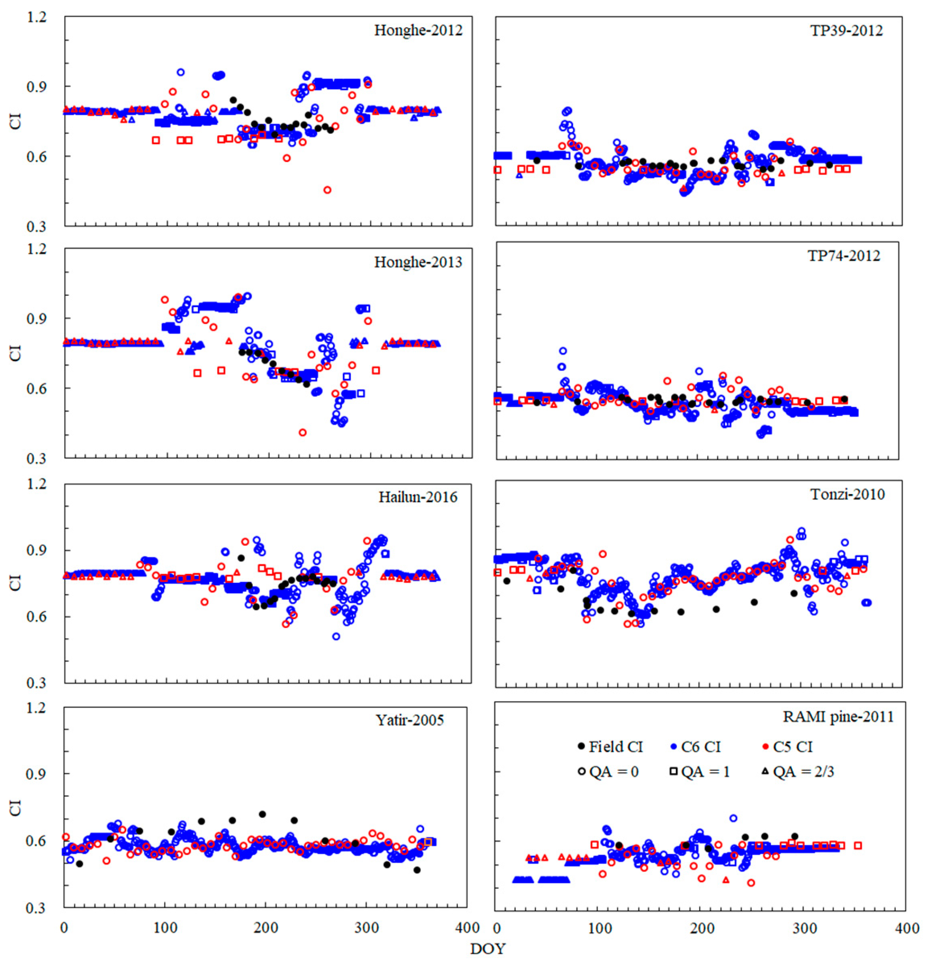
3.2.2. Evaluation of Seasonal Variability

Figure 7 shows the seasonal variabilities in the C5 8-day CI (red), C6 daily CI (blue), and field CI (black) data for the 7 field sites with seasonal profiles of field-measured CIs (Table 2). All valid MODIS CI values from the field sites during the field measurement year are shown, including the main algorithm (circles and squares denote retrievals of QA = 0 and 1, respectively) and backup algorithm (triangles) retrievals. Corresponding scatter plot for comparison of C5 8-day CI and C6 daily CI data with the field CI data can be found in Supplementary Materials (Figure S1).

In general, seasonal variations in the C5 and C6 MODIS CI data agree with the field-measured CIs, which reflect the states of vegetation growth and its intrinsic structures to some extent. The C6 CI data are closer overall to the field-measured CIs than the C5 CI data, while the C6 CI data present more temporal details and fluctuations due to their higher temporal resolutions. Both versions of the MODIS CI data and field-measured CI data show lower CI values (0.4–0.8) and small seasonal variations at evergreen conifer forest sites (i.e., TP39, TP74, Yatir, and RAMI pine) and higher CI values (0.5–1.0) and strong seasonal variations at cropland sites (i.e., Honghe and Hailun) and woody savanna sites (i.e., Tonzi), which are consistent with previous studies [30,47,89,100]. The relatively small seasonal change in the CIs for coniferous forests may be attributed to the low needle turnover rate [47,101]. For the TP39, TP74, and RAMI pine sites, the field-measured CIs are stable at approximately 0.55, while the C5 and C6 CIs fluctuate at approximately 0.55, and the C6 CIs are closer to the field-measured CIs than the C5 CIs. For the two cropland sites, field data were mainly collected in the growing season (days of year (DOYs) 170–240), and both the C5 and C6 CIs showed seasonal variations similar to the field-measured CI data, which exhibited lower CI values during the peak growing period and higher CI values at the beginning and end of the growing season [30]. At the Honghe site, paddy rice is usually transplanted in May (DOYs 120–150) with higher CI values, and subsequently, the CI values decrease with vegetation growth and return to higher values after the rice harvest in late August (DOYs 230–240). At the Hailun site, crops are generally sown in May with relatively high CI values, and then, the CI values decrease in June (DOYs 150–180) with vegetation growth and increase in July and August (DOYs 200–230) during the tasseling and milking stages; finally, they slightly increase in the mature stage in September (DOYs 240–270). In the fallow period, except for the freeze period (late October to April), the two versions of the MODIS CIs show relatively strong fluctuations before (DOYs 70–100) and after (DOYs 260–300) the growing season, which may be associated with the uncertainties in the corresponding MODIS BRDF data. The quality of MODIS BRDF data may be influenced by the increased heterogeneity of surface reflectivity before and after the growing season [108] and the poor angular sampling away from the principal plane in winter [109].

While the MODIS CIs generally follow the same trend as the field-measured CIs, there are some deviations in values, especially for the Yatir and Tonzi sites which have relatively sparse canopy distributions. The MODIS CIs mainly respond to the top structure of vegetation, while the field-measured CIs are usually influenced by understory vegetation [25,99]. At the Yatir sites, the field-measured CIs are higher (~0.7) in the middle of the year and lower (~0.5) at the beginning and end of the year, while the C5 and C6 CIs undulate at approximately 0.6. This site is located between arid and semiarid climatic zones, and the forest usually consists of individual canopies for the limited available water [83]. The relatively low field-measured CI values at the beginning and end of the year may be associated with the vegetation developed during the rainy season. At the Tonzi site, both versions of the MODIS CI data and field-measured CIs are lower from April to June and higher at the beginning and end of the year. This site generally consists of two layers of vegetation, a tree overstory and grass understory, that operate in and out of phase with each other over the course of a year [80,110]. The CI values decrease during DOYs 1–120, keeping pace with the growth of tree leaves, and the values increase slowly from the dry season until November (beginning of the rainy season). While the MODIS-derived CIs capture the overall trend of the seasonal variation caused by vegetation phenology, the satellite CI retrievals somewhat overestimate field-measured CIs [47,89]. The inconsistency between field-measured CIs and MODIS-derived CIs may be caused by the large difference in spatial scale between field measurements and satellite observations, as well as the influence of the change in background reflectance.

4. Discussion

4.1. Uncertainty in the MODIS CI Retrievals

The quality of MODIS-derived CI data relies heavily on the quality of input data (i.e., the MCD43A1/A2 and MCD12Q1 products) and the configuration of the retrieval algorithm. By using the improved MODIS C6 surface reflectance and cloud mask products and the enhanced daily retrieval algorithm, the C6 MCD43 products present improved data quality compared with the C5 products [35]. Correspondingly, the C6 CI data exhibit a higher proportion of main algorithm inversion and a lower proportion of missing values than the C5 CI data globally. The C6 CI data are also more consistent with the field-measured CI data than the C5 CI data are. Moreover, the input MCD12Q1 IGBP land cover data determine the crown shape in the retrieval algorithm and thus influence the accuracy of the CI data [25]. The land cover map provides the basic distribution pattern of the global CI data, as the needleleaf forest comprises shoot level clumping rather than the leaf element level clumping in broadleaf vegetation types. As the accuracy of the BRDF product has been implied by the CI QA data, caution should be exercised when determining the uncertainty of land cover data in the utilization of the CI product.

In addition to the uncertainties of the input data, the configuration of the retrieval algorithm is also crucial to the accuracy of the MODIS CI data. As the RTLSR BRDF model used in the operational MODIS BRDF inversion algorithm reportedly underestimates the reflectance at the hotspot [25,89], the RTCLSR model [74] is used in this study. The RTCLSR BRDF model rebuilds the hotspot magnitude and width with two parameters based on an exponential approximation of a physical hotspot kernel, which corrects the hotspot signatures with high accuracy and without distinct scale dependence [26]. The linear CI-NDHD equations have been widely used to retrieve global CI maps [25,28,29,30,111] and are considered to be the best guess for the surface CI [24,26]. As the CI-NDHD relationships are affected by sparse vegetation coverage and high background reflectance, uncertainties in the CI data in these circumstances should be treated with some caution [24,25,47]. Furthermore, terrain-induced shadows can also increase the uncertainty of CI retrievals, which deserves further investigation [24,49,111].

4.2. Uncertainty in Field-Measured CI Data

The field-measured CI data used in this study are collected from different sources, and uncertainties arising from different observational instruments and methods should be considered an error source in validating the MODIS CI data. The field measurement of CI data is usually based on observations of transmitted light of the canopy by using instruments, such as TRAC [77,112] and DHP [113,114]. Various methods have been developed to estimate the CI data from field measurements, such as the method based on gap size distribution [77] and its corrected method [112], the logarithmic average method [115], and the combined gap size and logarithm method [90]. While previous studies reported a high correlation among different methods, observations with different view zenith angles, the assumption of the leaf projection function and the segment size may influence the assessment of field CI values [76,116]. Moreover, the measurement conditions, such as sunlight, terrain, and observation height, may also influence the correct estimation of the field CI [76,117].

The different spatial scales of field-measured CI data and MODIS-derived CI data may introduce scaling errors when validating the MODIS CI data [25,78,89]. Generally, field-measured data are optimally integrated with high-resolution data to validate moderate-resolution products [118,119]. As there are no adequate high-resolution CI data to conduct this validation strategy, the homogeneity and representativeness of field sites are usually used to assess the field-measured CI data and reduce spatial scaling errors [25,26,29,49]. While these assessments of sites are limited by the use of high-resolution single-angular reflectance data, further studies with high-resolution multiangle data and retrieved CI data are urgently needed to perform comprehensive validations of moderate-resolution CI data.

4.3. Seasonal Variability in the CI

The results of this study indicate that the seasonal variability in the CI data has the potential to reflect the change in vegetation status, which confirms the results of previous studies [30,47,70,99,100]. While the variation in the CI is closely related to the LAI, which exhibits low CI values in the growing season and high values in the dormant period, the tree cover, canopy arrangement, understory vegetation, and background reflectance all contribute to the seasonal variation in the CI [7,30,47]. Compared with 8-day and daily CIs, the monthly CIs reduce the influence of poor-quality data and ephemeral background reflectance changes that can provide relatively reasonable surface CIs for ecological and meteorological modeling at global and regional scales.

Moreover, the spatial and temporal mismatch of field-measured CIs and retrieved MODIS CIs most likely lead to inconsistencies in the evaluation of seasonal variabilities. As seen in 7 sites with seasonal profiles of field-measured CIs, compared to field-measured CI data, satellite-derived CIs with larger spatial extents are more susceptible to changes in the surrounding and background reflectance in theory [47]. In addition, satellite data mainly respond to the top structure of vegetation, while the field-measured CIs are probably influenced by understory vegetation. Field-measured CIs influenced by understory vegetation may overestimate the forest CIs, as the CIs of shrubs are usually higher than those of trees [25,99]. These issues propose a huge challenge for the validation of satellite CI retrievals using field CI measurements.

The different temporal scales of the C5 8-day CIs, C6 daily Cis, and field-measured CIs should be considered sources of uncertainty in the comparison of seasonal variability. The temporal resolutions of the C5 8-day and C6 daily CI data are the same as those of the corresponding BRDF products. Both the C5 and C6 BRDF products are produced by using observations accumulated in a 16-day period, while the C5 algorithm retrieves data every 8 days with the first day being the day of interest, and the C6 algorithm retrieves data every day with the central day being the day of interest [35]. These temporal differences between the C5 CIs, C6 CIs, and field CIs may introduce temporal bias in the comparison of CI seasonal variations.

5. Conclusions

The CI is a crucial vegetation structure parameter that plays an important role in LAI estimations and the building of ecological, hydrological, and land surface models. Its seasonality is also critical in LAI mapping and ecosystem modeling. The MODIS BRDF/Albedo product is the most widely used input data for CI retrieval. As the newly released C6 product presents significant improvements in data quality and temporal resolution, it is imperative for the application of MODIS CI products to determine the impacts of updating the MCD43 product as an important input for the consistency and performance of CI retrievals. In this study, CI retrievals from the C5 and C6 MCD43 products were compared and validated in terms of spatial distributions and seasonal variations. The results are described as follows:

(1)

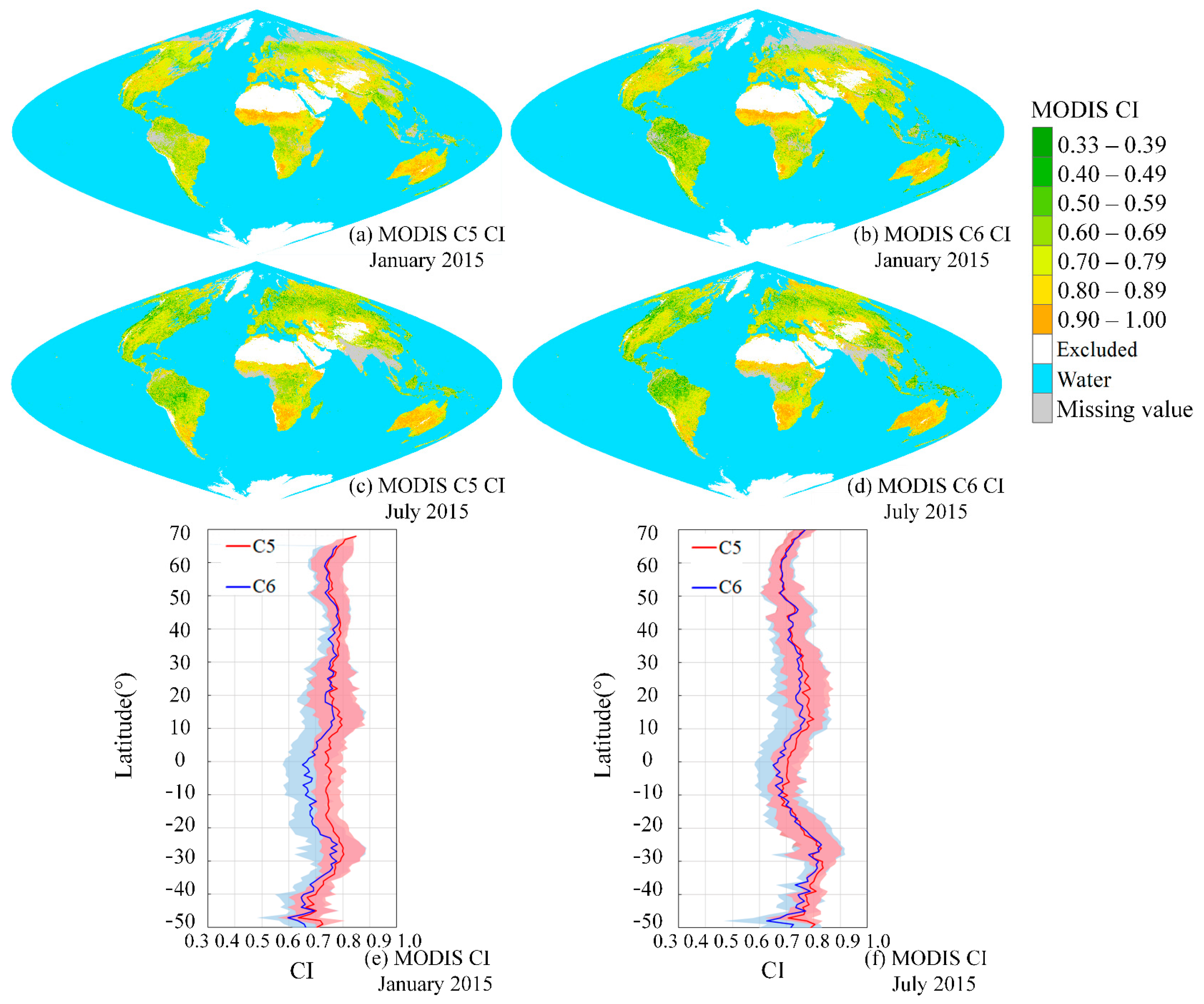
The C5 and C6 CI data show similar spatial distributions globally. These two versions of data exhibit similar spatial patterns and latitudinal distributions globally in January and July, which relate to the distribution of vegetation types and leaf-on/leaf-off seasons. Forest areas have lower CI values, while grass, shrub, crop, and savanna regions display higher CI values. In the Northern Hemisphere, the January CI is generally higher than that in July, and the opposite is true in the Southern Hemisphere.

(2)

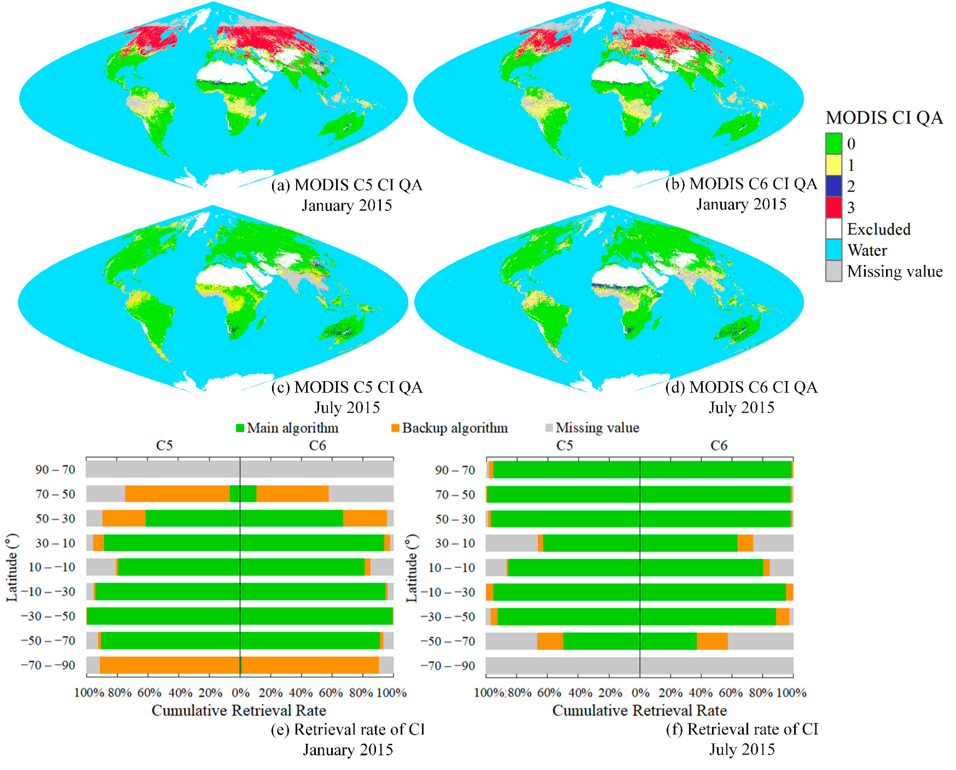
The C5 and C6 CI QA data show similar patterns globally, while the C6 CI data have an improved quality with more main algorithm retrievals and fewer missing values. For both versions of data, the overall proportion of main algorithm retrievals is higher in July than in January, while the C6 data show a higher rate of main algorithm retrievals and a lower rate of missing value in the summer hemisphere and a lower rate of backup algorithm retrieval in most of the world.

(3)

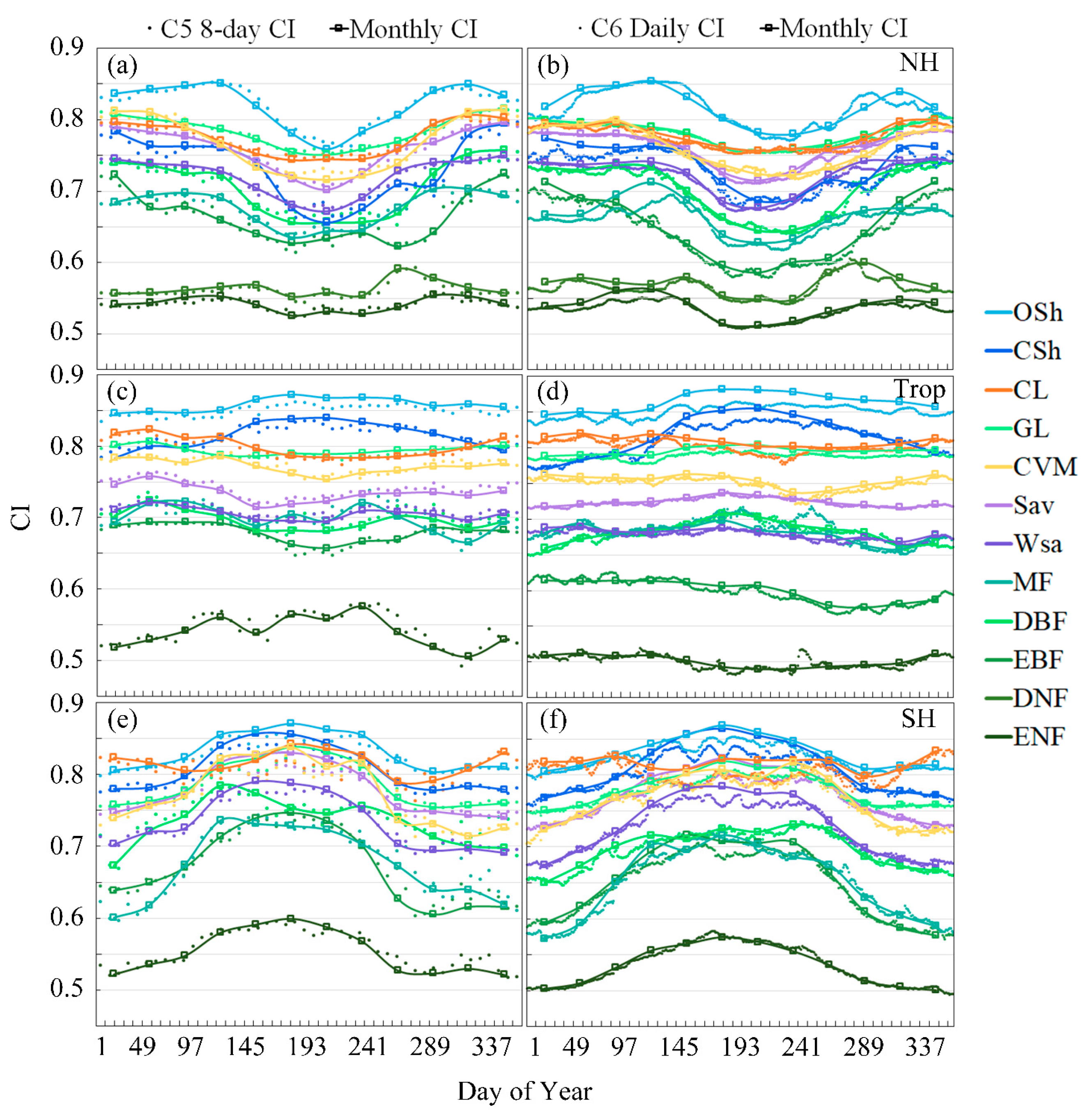
In general, the C5 and C6 CI data show similar seasonal variations in the three latitude zones (NH, SH, and Trop) and different land cover types, which is consistent with the vegetation phenology. Through quality screening and averaging, the monthly CI data have higher data quality and are recommended to characterize the overall seasonal patterns of the surface CIs well, with less uncertainty than using C5 8-day, monthly, and C6 daily CI data.

(4)

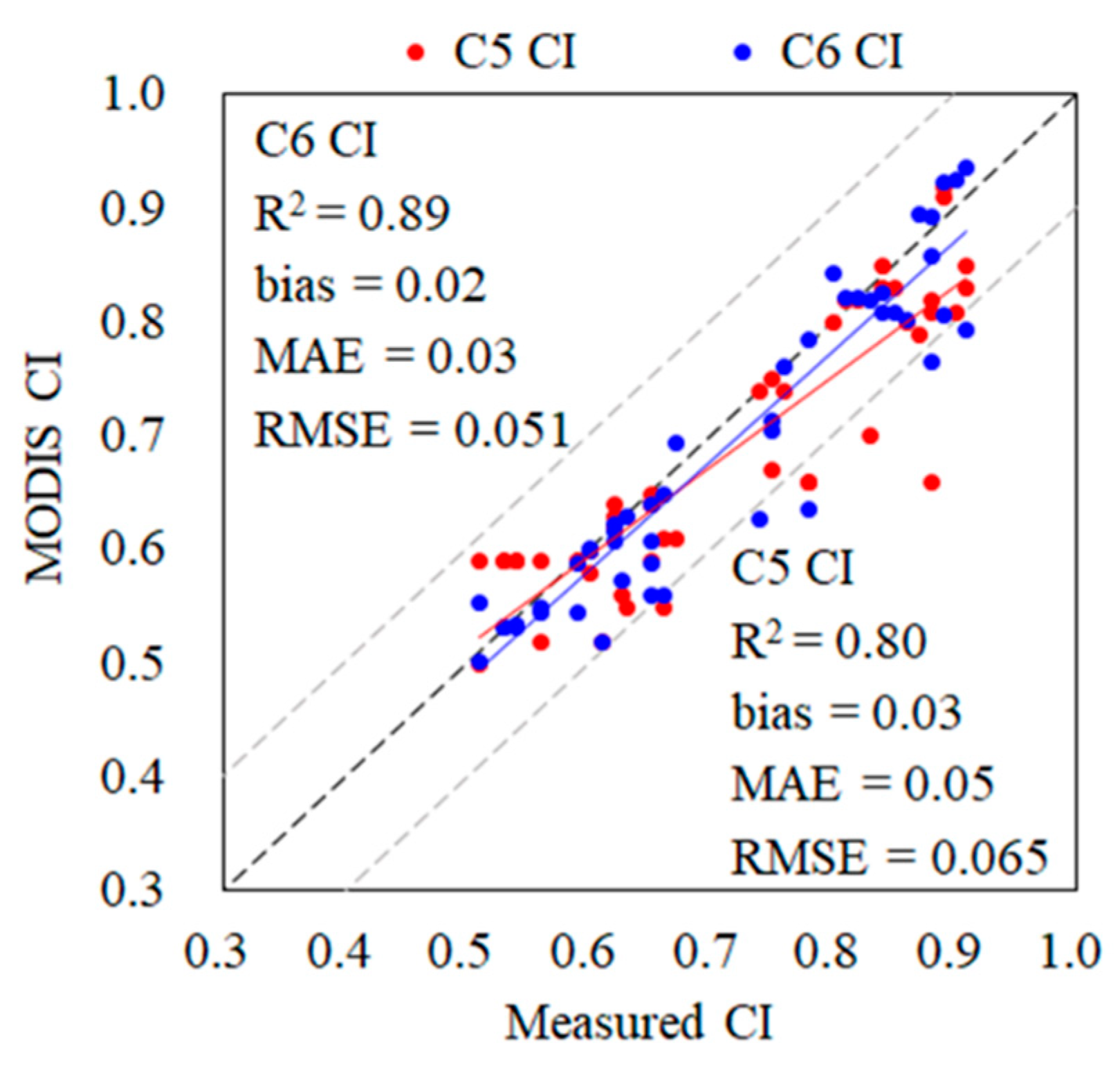
Through a comparison with field-measured CI data, both versions of the MODIS CI data agree with the field-measured CIs and their seasonal variations, while the C6 CI data (R² = 0.89, RMSE = 0.05, bias = 0.02) show better consistency with the field measurements than the C5 CI data (R² = 0.80, RMSE = 0.07, bias = 0.03).

Remote sensing CI retrieval products are susceptible to the performance of upstream data. Comprehensive evaluation and analysis of updated derived data as input are crucial for choosing the correct and reasonable CI products for downstream applications for user communities. As improvements in remote sensing instruments and processing algorithms are ongoing, further studies are needed for updated products, such as the MODIS C6.1 product and even the Visible Infrared Imaging Radiometer Suite (VIIRS) BRDF/Albedo product [120]. In addition, the within-pixel variability of CI measurements in satellite CI product validation and the influence of spatial resolution on CI retrievals from different satellite sensors deserve to be further explored in near future.

References

1. Chen, J.M.; Black, T.A. Foliage area and architecture of plant canopies from sunfleck size distributions. Agric. For. Meteorol. 1992, 60, 249–266. [Google Scholar] [CrossRef]
2. Nilson, T. Theoretical analysis of frequency of gaps in plant stands. Agric. Meteorol. 1971, 8, 25–38. [Google Scholar] [CrossRef]
3. Wilson, J.W. Analysis of the spatial distribution of foliage by two-dimensional point quadrats. New Phytol. 1959, 58, 92–99. [Google Scholar] [CrossRef]
4. Duthoit, S.; Demarez, V.; Gastellu-Etchegorry, J.P.; Martin, E.; Roujean, J.L. Assessing the effects of the clumping phenomenon on BRDF of a maize crop based on 3D numerical scenes using DART model. Agric. For. Meteorol. 2008, 148, 1341–1352. [Google Scholar] [CrossRef]
5. Chen, B.; Liu, J.; Chen, J.M.; Croft, H.; Gonsamo, A.; He, L.; Luo, X. Assessment of foliage clumping effects on evapotranspiration estimates in forested ecosystems. Agric. For. Meteorol. 2016, 216, 82–92. [Google Scholar] [CrossRef]
6. Chen, J.M.; Mo, G.; Pisek, J.; Liu, J.; Deng, F.; Ishizawa, M.; Chan, D. Effects of foliage clumping on the estimation of global terrestrial gross primary productivity. Glob. Biogeochem. Cycles 2012, 26, 18. [Google Scholar] [CrossRef]
7. Hill, M.J.; Roman, M.O.; Schaaf, C.B.; Hutley, L.; Brannstrom, C.; Etter, A.; Hanan, N.P. Characterizing vegetation cover in global savannas with an annual foliage clumping index derived from the MODIS BRDF product. Remote Sens. Environ. 2011, 115, 2008–2024. [Google Scholar] [CrossRef]
8. Chen, J.M.; Black, T.A. Measuring Leaf-Area Index of Plant Canopies with Branch Architecture. Agric. For. Meteorol. 1991, 57, 1–12. [Google Scholar] [CrossRef]
9. Pisek, J.; Chen, J.M.; Alikas, K.; Deng, F. Impacts of including forest understory brightness and foliage clumping information from multiangular measurements on leaf area index mapping over North America. J. Geophys. Res.-Biogeosci. 2010, 115, 13. [Google Scholar] [CrossRef]
10. Zhu, X.; Skidmore, A.K.; Wang, T.J.; Liu, J.; Darvishzadeh, R.; Shi, Y.F.; Premier, J.; Heurich, M. Improving leaf area index (LAI) estimation by correcting for clumping and woody effects using terrestrial laser scanning. Agric. For. Meteorol. 2018, 263, 276–286. [Google Scholar] [CrossRef]
11. Stenberg, P. Correcting LAI-2000 estimates for the clumping of needles in shoots of conifers. Agric. For. Meteorol. 1996, 79, 1–8. [Google Scholar] [CrossRef]
12. Chen, J.M.; Liu, J.; Leblanc, S.G.; Lacaze, R.; Roujean, J.L. Multi-angular optical remote sensing for assessing vegetation structure and carbon absorption. Remote Sens. Environ. 2003, 84, 516–525. [Google Scholar] [CrossRef]
13. Chen, B.; Lu, X.H.; Wang, S.Q.; Chen, J.M.; Liu, Y.; Fang, H.L.; Liu, Z.H.; Jiang, F.; Arain, M.A.; Chen, J.H.; et al. Evaluation of Clumping Effects on the Estimation of Global Terrestrial Evapotranspiration. Remote Sens. 2021, 13, 4075. [Google Scholar] [CrossRef]
14. Chen, J.M.; Ju, W.M.; Ciais, P.; Viovy, N.; Liu, R.G.; Liu, Y.; Lu, X.H. Vegetation structural change since 1981 significantly enhanced the terrestrial carbon sink. Nat. Commun. 2019, 10, 7. [Google Scholar] [CrossRef]
15. Anderson, M.C.; Norman, J.M.; Kustas, W.P.; Li, F.Q.; Prueger, J.H.; Mecikalski, J.R. Effects of vegetation clumping on two-source model estimates of surface energy fluxes from an agricultural landscape during SMACEX. J. Hydrometeorol. 2005, 6, 892–909. [Google Scholar] [CrossRef]
16. Chen, H.Y.; Niu, Z.; Huang, W.J.; Feng, J.L. Predicting leaf area index in wheat using an improved empirical model. J. Appl. Remote Sens. 2013, 7, 073577. [Google Scholar] [CrossRef]
17. Roujean, J.L.; Lacaze, R. Global mapping of vegetation parameters from POLDER multiangular measurements for studies of surface-atmosphere interactions: A pragmatic method and its validation. J. Geophys. Res.-Atmos. 2002, 107, 20. [Google Scholar] [CrossRef]
18. Gobron, N.; Pinty, B.; Verstraete, M.M.; Widlowski, J.L.; Diner, D.J. Uniqueness of multiangular measurements—Part II: Joint retrieval of vegetation structure and photosynthetic activity from MISR. IEEE Trans. Geosci. Remote Sens. 2002, 40, 1574–1592. [Google Scholar] [CrossRef]
19. Strahler, A.H. Vegetation canopy reflectance modeling—Recent developments and remote sensing perspectives. Remote Sens. Rev. 1997, 15, 179–194. [Google Scholar] [CrossRef]
20. Nicodemus, F.E.; Richmond, J.C.; Hsia, J.J.; Ginsberg, I.W.; Limperis, T. Geometrical Considerations and Nomenclature for Reflectance; U.S. Department of Commerce: Washington, DC, USA, 1977. [CrossRef]
21. Schaaf, C.B.; Gao, F.; Strahler, A.H.; Lucht, W.; Li, X.W.; Tsang, T.; Strugnell, N.C.; Zhang, X.Y.; Jin, Y.F.; Muller, J.P.; et al. First operational BRDF, albedo nadir reflectance products from MODIS. Remote Sens. Environ. 2002, 83, 135–148. [Google Scholar] [CrossRef]
22. Jiao, Z.T.; Hill, M.J.; Schaaf, C.B.; Zhang, H.; Wang, Z.S.; Li, X.W. An Anisotropic Flat Index (AFX) to derive BRDF archetypes from MODIS. Remote Sens. Environ. 2014, 141, 168–187. [Google Scholar] [CrossRef]
23. Leblanc, S.G.; Chen, J.M.; White, H.P.; Cihlar, J.; Lacaze, R.; Roujean, J.-L.; Latifovic, R. Mapping vegetation Clumping index from directional satellite measurements. In Proceedings of the 8th International Symposium Physical Measurements & Signatures in Remote Sensing, Aussois, France, 8–12 January 2001; pp. 450–459. [Google Scholar]
24. Chen, J.M.; Menges, C.H.; Leblanc, S.G. Global mapping of foliage clumping index using multi-angular satellite data. Remote Sens. Environ. 2005, 97, 447–457. [Google Scholar] [CrossRef]
25. He, L.M.; Chen, J.M.; Pisek, J.; Schaaf, C.B.; Strahler, A.H. Global clumping index map derived from the MODIS BRDF product. Remote Sens. Environ. 2012, 119, 118–130. [Google Scholar] [CrossRef]
26. Jiao, Z.T.; Dong, Y.D.; Schaaf, C.B.; Chen, J.M.; Roman, M.; Wang, Z.S.; Zhang, H.; Ding, A.X.; Erb, A.; Hill, M.J.; et al. An algorithm for the retrieval of the clumping index (CI) from the MODIS BRDF product using an adjusted version of the kernel-driven BRDF model. Remote Sens. Environ. 2018, 209, 594–611. [Google Scholar] [CrossRef]
27. Leblanc, S.G.; Chen, J.M.; White, H.P.; Latifovic, R.; Lacaze, R.; Roujean, J.-L. Canada-wide foliage clumping index mapping from multiangular POLDER measurements. Can. J. Remote Sens. 2005, 31, 364–376. [Google Scholar] [CrossRef]
28. Pisek, J.; Chen, J.M.; Nilson, T. Estimation of vegetation clumping index using MODIS BRDF data. Int. J. Remote Sens. 2011, 32, 2645–2657. [Google Scholar] [CrossRef]
29. Wei, S.S.; Fang, H.L. Estimation of canopy clumping index from MISR and MODIS sensors using the normalized difference hotspot and darkspot (NDHD) method: The influence of BRDF models and solar zenith angle. Remote Sens. Environ. 2016, 187, 476–491. [Google Scholar] [CrossRef]
30. Wei, S.S.; Fang, H.L.; Schaaf, C.B.; He, L.M.; Chen, J.M. Global 500 m clumping index product derived from MODIS BRDF data (2001–2017). Remote Sens. Environ. 2019, 232, 15. [Google Scholar] [CrossRef]
31. Schaaf, C.B.; Wang, Z.; Strahler, A.H. Commentary on Wang and Zender-MODIS snow albedo bias at high solar zenith angles relative to theory and to in situ observations in Greenland. Remote Sens. Environ. 2011, 115, 1296–1300. [Google Scholar] [CrossRef]
32. Lucht, W.; Schaaf, C.B.; Strahler, A.H. An algorithm for the retrieval of albedo from space using semiempirical BRDF models. IEEE Trans. Geosci. Remote Sens. 2000, 38, 977–998. [Google Scholar] [CrossRef]
33. Roujean, J.L.; Leroy, M.; Deschamps, P.Y. A bidirectional reflectance model of the earths surface for the correction of remote-sensing data. J. Geophys. Res.-Atmos. 1992, 97, 20455–20468. [Google Scholar] [CrossRef]
34. Wanner, W.; Li, X.; Strahler, A.H. On the derivation of kernels for kernel-driven models of bidirectional reflectance. J. Geophys. Res.-Atmos. 1995, 100, 21077–21089. [Google Scholar] [CrossRef]
35. Wang, Z.S.; Schaaf, C.B.; Sun, Q.S.; Shuai, Y.M.; Roman, M.O. Capturing rapid land surface dynamics with Collection V006 MODIS BRDF/NBAR/Albedo (MCD43) products. Remote Sens. Environ. 2018, 207, 50–64. [Google Scholar] [CrossRef]
36. Schaaf, C. MODIS User Guide V006 and V006.1. Available online: https://www.umb.edu/spectralmass/terra_aqua_modis/v006 (accessed on 16 December 2021).
37. Xiong, X.X.; Angal, A.; Li, Y.H.; Twedt, K. Improvements of on-orbit characterization of Terra MODIS short-wave infrared spectral bands out-of-band responses. J. Appl. Remote Sens. 2020, 14, 14. [Google Scholar] [CrossRef]
38. Toller, G.; Xiong, X.X.; Sun, J.Q.; Wenny, B.N.; Geng, X.; Kuyper, J.; Angal, A.; Chen, H.D.; Madhavan, S.; Wu, A.S. Terra and Aqua moderate-resolution imaging spectroradiometer collection 6 level 1B algorithm. J. Appl. Remote Sens. 2013, 7, 17. [Google Scholar] [CrossRef]
39. Cui, L.; Jiao, Z.T.; Dong, Y.D.; Sun, M.; Zhang, X.N.; Yin, S.Y.; Ding, A.X.; Chang, Y.X.; Guo, J.; Xie, R. Estimating Forest Canopy Height Using MODIS BRDF Data Emphasizing Typical-Angle Reflectances. Remote Sens. 2019, 11, 2239. [Google Scholar] [CrossRef]
40. Pisek, J.; Rautiainen, M.; Nikopensius, M.; Raabe, K. Estimation of seasonal dynamics of understory NDVI in northern forests using MODIS BRDF data: Semi-empirical versus physically-based approach. Remote Sens. Environ. 2015, 163, 42–47. [Google Scholar] [CrossRef]
41. Zhang, X.N.; Jiao, Z.T.; Zhao, C.S.; Yin, S.Y.; Cui, L.; Dong, Y.D.; Zhang, H.; Guo, J.; Xie, R.; Li, S.J.; et al. Retrieval of Leaf Area Index by Linking the PROSAIL and Ross-Li BRDF Models Using MODIS BRDF Data. Remote Sens. 2021, 13, 4911. [Google Scholar] [CrossRef]
42. Zhang, H.; Zhao, M.; Jiao, Z.; Lian, Y.; Chen, L.; Cui, L.; Zhang, X.; Liu, Y.; Dong, Y.; Qian, D.; et al. Reflectance Anisotropy from MODIS for Albedo Retrieval from a Single Directional Reflectance. Remote Sens. 2022, 14, 3627. [Google Scholar] [CrossRef]
43. Hu, P.B.; Sharifi, A.; Tahir, M.N.; Tariq, A.; Zhang, L.L.; Mumtaz, F.; Shah, S. Evaluation of Vegetation Indices and Phenological Metrics Using Time-Series MODIS Data for Monitoring Vegetation Change in Punjab, Pakistan. Water 2021, 13, 2550. [Google Scholar] [CrossRef]
44. Sarvia, F.; De Petris, S.; Borgogno-Mondino, E. Exploring Climate Change Effects on Vegetation Phenology by MOD13Q1 Data: The Piemonte Region Case Study in the Period 2001–2019. Agronomy 2021, 11, 555. [Google Scholar] [CrossRef]
45. Zhang, X.Y.; Friedl, M.A.; Schaaf, C.B.; Strahler, A.H.; Hodges, J.C.F.; Gao, F.; Reed, B.C.; Huete, A. Monitoring vegetation phenology using MODIS. Remote Sens. Environ. 2003, 84, 471–475. [Google Scholar] [CrossRef]
46. Zhang, X.Y.; Friedl, M.A.; Schaaf, C.B. Global vegetation phenology from Moderate Resolution Imaging Spectroradiometer (MODIS): Evaluation of global patterns and comparison with in situ measurements. J. Geophys. Res.-Biogeosci. 2006, 111, 14. [Google Scholar] [CrossRef]
47. He, L.M.; Liu, J.; Chen, J.M.; Croft, H.; Wang, R.; Sprintsin, M.; Zheng, T.R.; Ryu, Y.; Piseke, J.; Gonsamo, A.; et al. Inter- and intra-annual variations of clumping index derived from the MODIS BRDF product. Int. J. Appl. Earth Obs. Geoinf. 2016, 44, 53–60. [Google Scholar] [CrossRef]
48. Hill, M.J.; Averill, C.; Jiao, Z.; Schaaf, C.B.; Armston, J.D. Relationship of MISR RPV parameters and MODIS BRDF shape indicators to surface vegetation patterns in an Australian tropical savanna. Can. J. Remote Sens. 2008, 34, S247–S267. [Google Scholar] [CrossRef]
49. Zhu, G.; Ju, W.; Chen, J.M.; Gong, P.; Xing, B.; Zhu, J. Foliage Clumping Index Over China’s Landmass Retrieved From the MODIS BRDF Parameters Product. IEEE Trans. Geosci. Remote Sens. 2012, 50, 2122–2137. [Google Scholar] [CrossRef]
50. Liu, Y.; Liu, R.G.; Chen, J.M. Retrospective retrieval of long-term consistent global leaf area index (1981–2011) from combined AVHRR and MODIS data. J. Geophys. Res.-Biogeosci. 2012, 117, 14. [Google Scholar] [CrossRef]
51. Xiao, Z.Q.; Liang, S.L.; Wang, J.D.; Chen, P.; Yin, X.J.; Zhang, L.Q.; Song, J.L. Use of General Regression Neural Networks for Generating the GLASS Leaf Area Index Product From Time-Series MODIS Surface Reflectance. IEEE Trans. Geosci. Remote Sens. 2014, 52, 209–223. [Google Scholar] [CrossRef]
52. Gonsamo, A.; Chen, J.M. Improved LAI Algorithm Implementation to MODIS Data by Incorporating Background, Topography, and Foliage Clumping Information. IEEE Trans. Geosci. Remote Sens. 2014, 52, 1076–1088. [Google Scholar] [CrossRef]
53. Liu, L.; Zhang, X.; Xie, S.; Liu, X.; Song, B.; Chen, S.; Peng, D. Global White-Sky and Black-Sky FAPAR Retrieval Using the Energy Balance Residual Method: Algorithm and Validation. Remote Sens. 2019, 11, 1004. [Google Scholar] [CrossRef]
54. Zhao, J.; Li, J.; Liu, Q.; Xu, B.; Yu, W.; Lin, S.; Hu, Z. Estimating fractional vegetation cover from leaf area index and clumping index based on the gap probability theory. Int. J. Appl. Earth Obs. Geoinf. 2020, 90, 102112. [Google Scholar] [CrossRef]
55. Ryu, Y.; Baldocchi, D.D.; Kobayashi, H.; van Ingen, C.; Li, J.; Black, T.A.; Beringer, J.; van Gorsel, E.; Knohl, A.; Law, B.E.; et al. Integration of MODIS land and atmosphere products with a coupled-process model to estimate gross primary productivity and evapotranspiration from 1 km to global scales. Glob. Biogeochem. Cycles 2011, 25, 24. [Google Scholar] [CrossRef]
56. Zhang, F.; Chen, J.M.; Chen, J.; Gough, C.M.; Martin, T.A.; Dragoni, D. Evaluating spatial and temporal patterns of MODIS GPP over the conterminous U.S. against flux measurements and a process model. Remote Sens. Environ. 2012, 124, 717–729. [Google Scholar] [CrossRef]
57. He, L.M.; Chen, J.M.; Liu, J.; Mo, G.; Joiner, J. Angular normalization of GOME-2 Sun-induced chlorophyll fluorescence observation as a better proxy of vegetation productivity. Geophys. Res. Lett. 2017, 44, 5691–5699. [Google Scholar] [CrossRef]
58. Pu, J.B.; Yan, K.; Zhou, G.H.; Lei, Y.Q.; Zhu, Y.X.; Guo, D.H.; Li, H.L.; Xu, L.L.; Knyazikhin, Y.; Myneni, R.B. Evaluation of the MODIS LAI/FPAR Algorithm Based on 3D-RTM Simulations: A Case Study of Grassland. Remote Sens. 2020, 12, 3391. [Google Scholar] [CrossRef]
59. Verhoef, W. Bi-hemispherical Canopy Reflectance Model with Surface Heterogeneity Effects for the Estimation of LAI and fAPAR from MODIS White-Sky Spectral Albedo Data. Remote Sens. 2021, 13, 1976. [Google Scholar] [CrossRef]
60. Che, X.H.; Feng, M.; Sexton, J.O.; Channan, S.; Yang, Y.P.; Sun, Q. Assessment of MODIS BRDF/Albedo Model Parameters (MCD43A1 Collection 6) for Directional Reflectance Retrieval. Remote Sens. 2017, 9, 1123. [Google Scholar] [CrossRef]
61. Vidot, J.; Brunel, P.; Dumont, M.; Carmagnola, C.; Hocking, J. The VIS/NIR Land and Snow BRDF Atlas for RTTOV: Comparison between MODIS MCD43C1 C5 and C6. Remote Sens. 2018, 10, 21. [Google Scholar] [CrossRef]
62. Guerschman, J.P.; Hill, M.J. Calibration and validation of the Australian fractional cover product for MODIS collection 6. Remote Sens. Lett. 2018, 9, 696–705. [Google Scholar] [CrossRef]
63. Lucht, W.; Lewis, P. Theoretical noise sensitivity of BRDF and albedo retrieval from the EOS-MODIS and MISR sensors with respect to angular sampling. Int. J. Remote Sens. 2000, 21, 81–98. [Google Scholar] [CrossRef]
64. Ross, J. The Radiation Regime and Architecture of Plant Stands; Springer Science & Business Media: Hague, The Netherlands, 1981. [Google Scholar]
65. Li, X.W.; Strahler, A.H. Geometric-optical bidirectional refelectance modeling of the disctrete crown vegetation canopy—Effect of crown shape and mutual shadowing. IEEE Trans. Geosci. Remote Sens. 1992, 30, 276–292. [Google Scholar] [CrossRef]
66. Wolfe, R.E.; Roy, D.P.; Vermote, E. MODIS land data storage, gridding, and compositing methodology: Level 2 grid. IEEE Trans. Geosci. Remote Sens. 1998, 36, 1324–1338. [Google Scholar] [CrossRef]
67. Friedl, M.A.; Sulla-Menashe, D.; Tan, B.; Schneider, A.; Ramankutty, N.; Sibley, A.; Huang, X.M. MODIS Collection 5 global land cover: Algorithm refinements and characterization of new datasets. Remote Sens. Environ. 2010, 114, 168–182. [Google Scholar] [CrossRef]
68. Friedl, M.A.; McIver, D.K.; Hodges, J.C.F.; Zhang, X.Y.; Muchoney, D.; Strahler, A.H.; Woodcock, C.E.; Gopal, S.; Schneider, A.; Cooper, A.; et al. Global land cover mapping from MODIS: Algorithms and early results. Remote Sens. Environ. 2002, 83, 287–302. [Google Scholar] [CrossRef]
69. Sulla-Menashe, D.; Gray, J.M.; Abercrombie, S.P.; Friedl, M.A. Hierarchical mapping of annual global land cover 2001 to present: The MODIS Collection 6 Land Cover product. Remote Sens. Environ. 2019, 222, 183–194. [Google Scholar] [CrossRef]
70. Jiao, Z.T.; Zhang, X.N.; Breon, F.M.; Dong, Y.D.; Schaaf, C.B.; Roman, M.; Wang, Z.S.; Cui, L.; Yin, S.Y.; Ding, A.X.; et al. The influence of spatial resolution on the angular variation patterns of optical reflectance as retrieved from MODIS and POLDER measurements. Remote Sens. Environ. 2018, 215, 371–385. [Google Scholar] [CrossRef]
71. Chen, J.M.; Leblanc, S.G. A four-scale bidirectional reflectance model based on canopy architecture. IEEE Trans. Geosci. Remote Sens. 1997, 35, 1316–1337. [Google Scholar] [CrossRef]
72. Leblanc, S.G.; Bicheron, P.; Chen, J.M.; Leroy, M.; Cihlar, J. Investigation of directional reflectance in boreal forests with an improved four-scale model and airborne POLDER data. IEEE Trans. Geosci. Remote Sens. 1999, 37, 1396–1414. [Google Scholar] [CrossRef]
73. Chen, J.M.; Cihlar, J. A hotspot function in a simple bidirectional reflectance model for satellite applications. J. Geophys. Res.-Atmos. 1997, 102, 25907–25913. [Google Scholar] [CrossRef]
74. Jiao, Z.T.; Schaaf, C.B.; Dong, Y.D.; Roman, M.; Hill, M.J.; Chen, J.M.; Wang, Z.S.; Zhang, H.; Saenz, E.; Poudyal, R.; et al. A method for improving hotspot directional signatures in BRDF models used for MODIS. Remote Sens. Environ. 2016, 186, 135–151. [Google Scholar] [CrossRef]
75. Maignan, F.; Breon, F.M.; Lacaze, R. Bidirectional reflectance of Earth targets: Evaluation of analytical models using a large set of spaceborne measurements with emphasis on the Hot Spot. Remote Sens. Environ. 2004, 90, 210–220. [Google Scholar] [CrossRef]
76. Pisek, J.; Lang, M.; Nilson, T.; Korhonen, L.; Karu, H. Comparison of methods for measuring gap size distribution and canopy nonrandomness at Jarvselja RAMI (RAdiation transfer Model Intercomparison) test sites. Agric. For. Meteorol. 2011, 151, 365–377. [Google Scholar] [CrossRef]
77. Chen, J.M.; Cihlar, J. Plant canopy gap-size analysis theory for improving optical measurements of leaf-area index. Appl. Opt. 1995, 34, 6211–6222. [Google Scholar] [CrossRef] [PubMed]
78. Román, M.O.; Schaaf, C.B.; Woodcock, C.E.; Strahler, A.H.; Yang, X.Y.; Braswell, R.H.; Curtis, P.S.; Davis, K.J.; Dragoni, D.; Goulden, M.L.; et al. The MODIS (Collection V005) BRDF/albedo product: Assessment of spatial representativeness over forested landscapes. Remote Sens. Environ. 2009, 113, 2476–2498. [Google Scholar] [CrossRef]
79. Fang, H. Vegetation Structural Field Measurement Data for Northeastern China Crops (NECC); PANGAEA: Bremerhaven, Germany, 2021. [Google Scholar] [CrossRef]
80. Baldocchi, D.D.; Xu, L.; Kiang, N. How plant functional-type, weather, seasonal drought, and soil physical properties alter water and energy fluxes of an oak–grass savanna and an annual grassland. Agric. For. Meteorol. 2004, 123, 13–39. [Google Scholar] [CrossRef]
81. Kuusk, A.; Lang, M.; Kuusk, J. Database of optical and structural data for the validation of forest radiative transfer models. In Light Scattering Reviews 7: Radiative Transfer and Optical Properties of Atmosphere and Underlying Surface; Kokhanovsky, A.A., Ed.; Springer: Berlin/Heidelberg, Germany, 2013; pp. 109–148. [Google Scholar]
82. Peichl, M.; Arain, M.A.; Brodeur, J.J. Age effects on carbon fluxes in temperate pine forests. Agric. For. Meteorol. 2010, 150, 1090–1101. [Google Scholar] [CrossRef]
83. Sprintsin, M.; Cohen, S.; Maseyk, K.; Rotenberg, E.; Grunzweig, J.; Karnieli, A.; Berliner, P.; Yakir, D. Long term and seasonal courses of leaf area index in a semi-arid forest plantation. Agric. For. Meteorol. 2011, 151, 565–574. [Google Scholar] [CrossRef]
84. Grünzweig, J.M.; Lin, T.; Rotenberg, E.; Schwartz, A.; Yakir, D. Carbon sequestration in arid-land forest. Glob. Chang. Biol. 2003, 9, 791–799. [Google Scholar] [CrossRef]
85. Fang, H.L.; Zhang, Y.H.; Wei, S.S.; Li, W.J.; Ye, Y.C.; Sun, T.; Liu, W.W. Validation of global moderate resolution leaf area index (LAI) products over croplands in northeastern China. Remote Sens. Environ. 2019, 233, 19. [Google Scholar] [CrossRef]
86. Fang, H.L.; Li, W.J.; Wei, S.S.; Jiang, C.Y. Seasonal variation of leaf area index (LAI) over paddy rice fields in NE China: Intercomparison of destructive sampling, LAI-2200, digital hemispherical photography (DHP), and AccuPAR methods. Agric. For. Meteorol. 2014, 198, 126–141. [Google Scholar] [CrossRef]
87. Fang, H.L.; Ye, Y.C.; Liu, W.W.; Wei, S.S.; Ma, L. Continuous estimation of canopy leaf area index (LAI) and clumping index over broadleaf crop fields: An investigation of the PASTIS-57 instrument and smartphone applications. Agric. For. Meteorol. 2018, 253, 48–61. [Google Scholar] [CrossRef]
88. Weiss, M.; Baret, F. CAN-EYE V6.313 User Manual. Available online: http://www6.paca.inra.fr/can-eye/Documentation-Publications/Documentation (accessed on 23 September 2017).
89. Pisek, J.; Ryu, Y.; Sprintsin, M.; He, L.M.; Oliphant, A.J.; Korhonen, L.; Kuusk, J.; Kuusk, A.; Bergstrom, R.; Verrelst, J.; et al. Retrieving vegetation clumping index from-Multi-angle Imaging SpectroRadiometer (MISR) data at 275 m resolution. Remote Sens. Environ. 2013, 138, 126–133. [Google Scholar] [CrossRef]
90. Leblanc, S.G.; Chen, J.M.; Fernandes, R.; Deering, D.W.; Conley, A. Methodology comparison for canopy structure parameters extraction from digital hemispherical photography in boreal forests. Agric. For. Meteorol. 2005, 129, 187–207. [Google Scholar] [CrossRef]
91. Ryu, Y.; Verfaillie, J.; Macfarlane, C.; Kobayashi, H.; Sonnentag, O.; Vargas, R.; Ma, S.; Baldocchi, D.D. Continuous observation of tree leaf area index at ecosystem scale using upward-pointing digital cameras. Remote Sens. Environ. 2012, 126, 116–125. [Google Scholar] [CrossRef]
92. Macfarlane, C.; Hoffman, M.; Eamus, D.; Kerp, N.; Higginson, S.; McMurtrie, R.; Adams, M. Estimation of leaf area index in eucalypt forest using digital photography. Agric. For. Meteorol. 2007, 143, 176–188. [Google Scholar] [CrossRef]
93. Walcroft, A.S.; Brown, K.J.; Schuster, W.S.F.; Tissue, D.T.; Turnbull, M.H.; Griffin, K.L.; Whitehead, D. Radiative transfer and carbon assimilation in relation to canopy architecture, foliage area distribution and clumping in a mature temperate rainforest canopy in New Zealand. Agric. For. Meteorol. 2005, 135, 326–339. [Google Scholar] [CrossRef]
94. Iiames, J.S.; Congalton, R.; Pilant, A.; Lewis, T. Validation of an integrated estimation of loblolly pine (Pinus taeda L.) leaf area index (LAI) using two indirect optical methods in the southeastern United States. South. J. Appl. For. 2008, 32, 101–110. [Google Scholar] [CrossRef]
95. Iiames, J.S.; Pilant, A.; Lewis, T. In Situ Estimates of Forest LAI for MODIS Data Validation. In Remote Sensing and GIS Accuracy Assessment; CRC Press: Boca Raton, FL, USA, 2004; pp. 41–57. [Google Scholar]
96. Chen, J.M.; Govind, A.; Sonnentag, O.; Zhang, Y.Q.; Barr, A.; Amiro, B. Leaf area index measurements at Fluxnet-Canada forest sites. Agric. For. Meteorol. 2006, 140, 257–268. [Google Scholar] [CrossRef]
97. Sonnentag, O.; Talbot, J.; Chen, J.M.; Roulet, N.T. Using direct and indirect measurements of leaf area index to characterize the shrub canopy in an ombrotrophic peatland. Agric. For. Meteorol. 2007, 144, 200–212. [Google Scholar] [CrossRef]
98. Ryu, Y.; Sonnentag, O.; Nilson, T.; Vargas, R.; Kobayashi, H.; Wenk, R.; Baldocchi, D.D. How to quantify tree leaf area index in an open savanna ecosystem: A multi-instrument and multi-model approach. Agric. For. Meteorol. 2010, 150, 63–76. [Google Scholar] [CrossRef]
99. Pisek, J.; Govind, A.; Arndt, S.K.; Hocking, D.; Wardlaw, T.J.; Fang, H.; Matteucci, G.; Longdoz, B. Intercomparison of clumping index estimates from POLDER, MODIS, and MISR satellite data over reference sites. ISPRS J. Photogramm. Remote Sens. 2015, 101, 47–56. [Google Scholar] [CrossRef]
100. Dong, Y.D.; Jiao, Z.T.; Yin, S.Y.; Zhang, H.; Zhang, X.N.; Cui, L.; He, D.D.; Ding, A.X.; Chang, Y.X.; Yang, S.T. Influence of Snow on the Magnitude and Seasonal Variation of the Clumping Index Retrieved from MODIS BRDF Products. Remote Sens. 2018, 10, 1194. [Google Scholar] [CrossRef]
101. He, L.; Chen, J.M.; Pan, Y.; Birdsey, R.; Kattge, J. Relationships between net primary productivity and forest stand age in U.S. forests. Glob. Biogeochem. Cycles 2012, 26, GB3009. [Google Scholar] [CrossRef]
102. Van Stan II, J.T.; Coenders-Gerrits, M.; Dibble, M.; Bogeholz, P.; Norman, Z. Effects of phenology and meteorological disturbance on litter rainfall interception for a Pinus elliottii stand in the Southeastern United States. Hydrol. Process. 2017, 31, 3719–3728. [Google Scholar] [CrossRef]
103. Gao, Y.; Wang, W.; Liu, X.; Zhang, L.; Dend, F.; Yang, C.; Sun, Q. Evaluation of Carbon Sequestration of Forest Ecosystem in Xiamen City. Res. Environ. Sci. 2019, 32, 2001–2007. [Google Scholar]
104. Wang, Z.S.; Schaaf, C.B.; Chopping, M.J.; Strahler, A.H.; Wang, J.D.; Roman, M.O.; Rocha, A.V.; Woodcock, C.E.; Shuai, Y.M. Evaluation of Moderate-resolution Imaging Spectroradiometer (MODIS) snow albedo product (MCD43A) over tundra. Remote Sens. Environ. 2012, 117, 264–280. [Google Scholar] [CrossRef]
105. Wang, Z.S.; Schaaf, C.B.; Strahler, A.H.; Chopping, M.J.; Roman, M.O.; Shuai, Y.M.; Woodcock, C.E.; Hollinger, D.Y.; Fitzjarrald, D.R. Evaluation of MODIS albedo product (MCD43A) over grassland, agriculture and forest surface types during dormant and snow-covered periods. Remote Sens. Environ. 2014, 140, 60–77. [Google Scholar] [CrossRef]
106. Wang, Z.S.; Schaaf, C.B.; Sun, Q.S.; Kim, J.; Erb, A.M.; Gao, F.; Roman, M.O.; Yang, Y.; Petroy, S.; Taylor, J.R.; et al. Monitoring land surface albedo and vegetation dynamics using high spatial and temporal resolution synthetic time series from Landsat and the MODIS BRDF/NBAR/albedo product. Int. J. Appl. Earth Obs. Geoinf. 2017, 59, 104–117. [Google Scholar] [CrossRef]
107. Strugnell, N.C.; Lucht, W. An algorithm to infer continental-scale albedo from AVHRR data, land cover class, and field observations of typical BRDFs. J. Clim. 2001, 14, 1360–1376. [Google Scholar] [CrossRef]
108. Jin, Y.F.; Schaaf, C.B.; Woodcock, C.E.; Gao, F.; Li, X.W.; Strahler, A.H.; Lucht, W.; Liang, S.L. Consistency of MODIS surface bidirectional reflectance distribution function and albedo retrievals: 2. Validation. J. Geophys. Res.-Atmos. 2003, 108, 15. [Google Scholar] [CrossRef]
109. Jin, Y.F.; Schaaf, C.B.; Gao, F.; Li, X.W.; Strahler, A.H.; Lucht, W.; Liang, S.L. Consistency of MODIS surface bidirectional reflectance distribution function and albedo retrievals: 1. Algorithm performance. J. Geophys. Res.-Atmos. 2003, 108, 13. [Google Scholar] [CrossRef]
110. Griffin, J.R. Oak woodland. In Terrestrial Vegetation of California; Barbour, M.G., Major, J., Eds.; California Native Plant Society: London, UK, 1988; pp. 383–415. [Google Scholar]
111. Pisek, J.; Chen, J.M.; Lacaze, R.; Sonnentag, O.; Alikas, K. Expanding global mapping of the foliage clumping index with multi-angular POLDER three measurements: Evaluation and topographic compensation. ISPRS J. Photogramm. Remote Sens. 2010, 65, 341–346. [Google Scholar] [CrossRef]
112. Leblanc, S.G. Correction to the plant canopy gap-size analysis theory used by the Tracing Radiation and Architecture of Canopies instrument. Appl. Opt. 2002, 41, 7667–7670. [Google Scholar] [CrossRef]
113. Chen, J.M.; Black, T.A.; Adams, R.S. Evaluation of hemispherical photography for determining plant-area index and geometry of a forest stand. Agric. For. Meteorol. 1991, 56, 129–143. [Google Scholar] [CrossRef]
114. Demarez, V.; Duthoit, S.; Baret, F.; Weiss, M.; Dedieu, G. Estimation of leaf area and clumping indexes of crops with hemispherical photographs. Agric. For. Meteorol. 2008, 148, 644–655. [Google Scholar] [CrossRef]
115. Lang, A.R.G.; Xiang, Y.Q. Estimation of leaf-area index from transmission of direct sunlight in discontinuous canopies. Agric. For. Meteorol. 1986, 37, 229–243. [Google Scholar] [CrossRef]
116. Fang, H.L.; Liu, W.W.; Li, W.J.; Wei, S.S. Estimation of the directional and whole apparent clumping index (ACI) from indirect optical measurements. ISPRS J. Photogramm. Remote Sens. 2018, 144, 1–13. [Google Scholar] [CrossRef]
117. Leblanc, S.G.; Chen, J.M.; Kwong, M. Tracing Radiation and Architecture of Canopies (TRAC) Manual. TRAC MANUAL Version 2.1.4; Natural Resources Canada: Saint-Hubert, QC, Canada, 2005; pp. 12–13.
118. Fernandes, R.; Plummer, S.; Nightingale, J.; Baret, F.; Camacho, F.; Fang, H.; Garrigues, S.; Gobron, N.; Lang, M.; Lacaze, R.; et al. Global leaf area index product validation good practices. In Best Practice for Satellite-Derived Land Product Validation; Version 2.0; Schaepman-Strub, G., Román, M., Nickeson, J., Eds.; Land Product Validation Subgroup (WGCV/CEOS): Washington, DC, USA, 2014; p. 76. [Google Scholar]
119. Morisette, J.T.; Baret, F.; Privette, J.L.; Myneni, R.B.; Nickeson, J.E.; Garrigues, S.; Shabanov, N.V.; Weiss, M.; Fernandes, R.A.; Leblanc, S.G. Validation of global moderate-resolution LAI products: A framework proposed within the CEOS land product validation subgroup. IEEE Trans. Geosci. Remote Sens. 2006, 44, 1804–1817. [Google Scholar] [CrossRef]
120. Justice, C.O.; Roman, M.O.; Csiszar, I.; Vermote, E.F.; Wolfe, R.E.; Hook, S.J.; Friedl, M.; Wang, Z.S.; Schaaf, C.B.; Miura, T.; et al. Land and cryosphere products from Suomi NPP VIIRS: Overview and status. J. Geophys. Res.-Atmos. 2013, 118, 9753–9765. [Google Scholar] [CrossRef]
Figure 1. Distribution of collected field CI measurements for all IGBP classes at the global scale. The dots indicate 48 field-measured sites labeled with IDs listed in Table 1. The stars denote sites with seasonal profiles of field-measured CIs labeled with names in Table 2.
Remotesensing 14 03997 g001
Figure 2. Flow chart of the comparison of CI retrievals using two versions of MODIS BRDF products between C5 (red rectangles) and C6 (blue rectangles).
Remotesensing 14 03997 g002
Figure 3. Global distribution of CI retrieved from MODIS C5 and C6 MCD43 products in January and July 2015. Panels (ad) are color-coded global maps of the MODIS C6 and C5 CIs. The sinusoidal projection is used here. Panels (e) and (f) show the latitudinal distribution of the MODIS C5 and C6 CIs, respectively. The red and blue lines indicate C5 and C6 CIs, respectively, and the corresponding shaded area indicates the one standard deviation range.
Remotesensing 14 03997 g003
Figure 4. Global distribution of CI quality assurance (QA) data of the MODIS C5 and C6 CI products in January and July 2015. Panels (ad) are global maps of the CI quality flags corresponding to the CI maps in Figure 2 (see Section 3.1.2 for more details). Panels (e,f) show the latitudinal distribution of the retrieval rates of different algorithm paths in January (e) and July (f) 2015. Possible algorithm paths include the main algorithm (green), backup algorithm (red), and missing value (not retrieved, gray). These statistics exclude non-vegetation areas (15-Snow and Ice, 16-Barren) according to the MODIS IGBP land cover data.
Remotesensing 14 03997 g004
Figure 5. Seasonal variations in the MODIS C5 (a,c,e) and C6 (b,d,f) CIs averaged over the Northern Hemisphere (NH, 30–90°N), Southern Hemisphere (SH, 30–90°S), and tropics (Trop, 30°S–30°N) for different IGBP land cover types in 2015. The dots indicate variations in the C5 8-day CI and C6 daily CI, while the line with squares denotes variations in the monthly CI. ENF: evergreen needleleaf forests; DNF: deciduous needleleaf forests; EBF: evergreen broadleaf forests; DBF: deciduous broadleaf forests; MF: mixed forests; CSh: closed shrublands; OSh: open shrublands; WSa: woody savannas; Sav: savannas; GL: grasslands; CL: croplands; CVM: cropland/natural vegetation mosaics.
Remotesensing 14 03997 g005
Figure 6. Comparison between the monthly C5 and C6 CI retrievals and field measurements. Details of the field CI data are shown in Table 1. The red and blue dots indicate the C5 and C6 CIs, respectively. Solid regression lines represent the linear fits of the field-measured CIs with the MODIS CIs, which shows a higher accuracy acquired by using the updated version of upstream MODIS BRDF/albedo products.
Remotesensing 14 03997 g006
Figure 7. Comparison of seasonal variabilities in the C5 8-day CI and C6 daily CI with the field CI data. Details of the field CI data are shown in Table 2. Black dots denote the field CI data. Red and blue symbols indicate the C5 and C6 CIs, respectively. Circle, square, and triangle symbols represent the quality of the MODIS CIs (i.e., C5 and C6 CIs), which are the best quality (QA = 0), good quality (QA = 1), and backup algorithm retrievals (QA = 2/3), respectively.
Remotesensing 14 03997 g007
Publisher’s Note: MDPI stays neutral with regard to jurisdictional claims in published maps and institutional affiliations.