
Coherence of Eddy Kinetic Energy Variation during Eddy Life Span to Low-Frequency Ageostrophic Energy
by
 , , ,
, , ,
Zhisheng Zhang
1, 
Lingling Xie
1,2,3,*,
Quanan Zheng
4,
Mingming Li
1,2,3 ,
,
Junyi Li
1,2,3 and
Min Li
1,2,3 1
Laboratory of Coastal Ocean Variation and Disaster Prediction, College of Ocean and Meteorology, Guangdong Ocean University, Zhanjiang 524088, China
2
Key Laboratory of Climate, Resources and Environments in Continent Shelf Sea and Deep Ocean (LCRE), Zhanjiang 524088, China
3
Key Laboratory of Space Ocean Remote Sensing and Applications (LORA), Ministry of Natural Resources, Beijing 100081, China
4
Department of Atmospheric and Oceanic Science, University of Maryland, College Park, MD 20742, USA
*
Author to whom correspondence should be addressed.
Remote Sens. 2022, 14(15), 3793; https://doi.org/10.3390/rs14153793
Submission received: 10 July 2022
/
Revised: 30 July 2022
/
Accepted: 4 August 2022
/
Published: 6 August 2022
Abstract
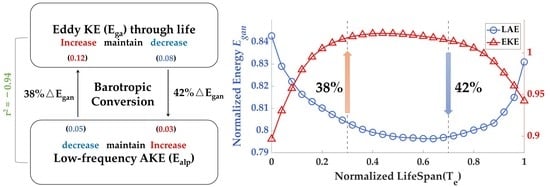
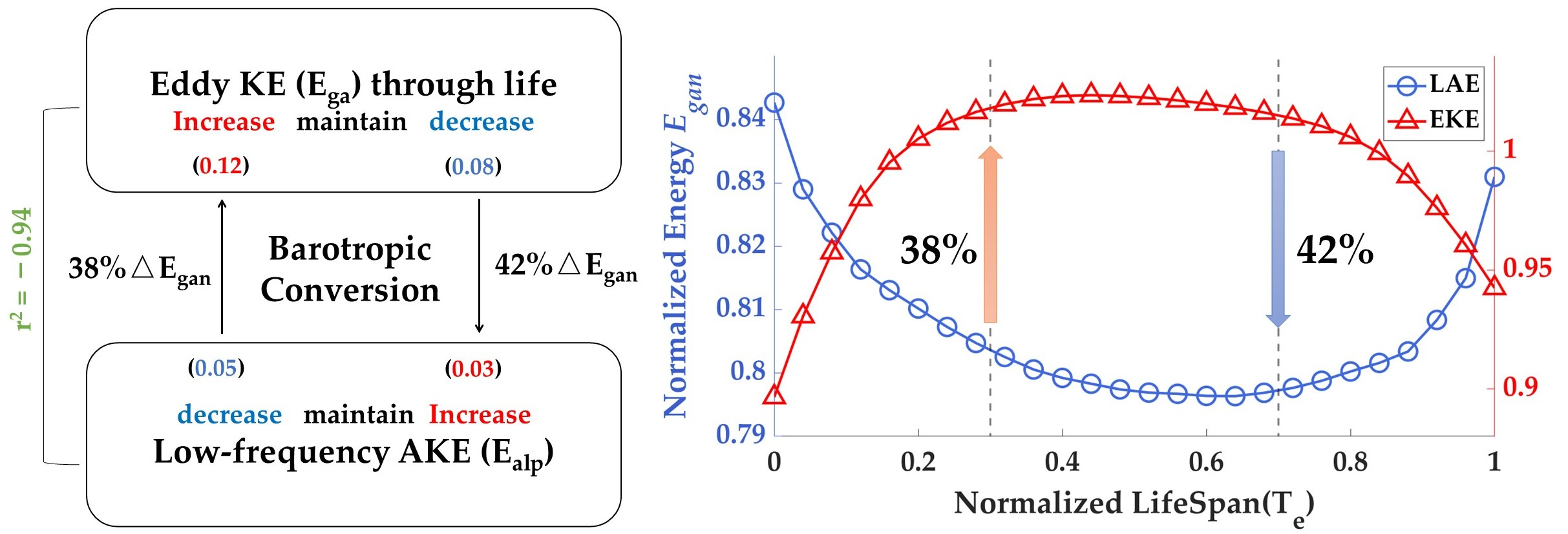
:The evolution of mesoscale eddies is crucial for understanding the ocean energy cascade. In this study, using global reanalysis sea surface velocity data and a mesoscale eddy trajectory product tracked by satellite altimeters, we aimed to reveal the coherence of eddy kinetic energy (EKE) variation to low-frequency ageostrophic energy during the eddy life span. The variation in EKE throughout the eddy life span was highly coherent to that of the seven-day low-passed ageostrophic kinetic energy, with a correlation coefficient of −0.94. The low-frequency ageostrophic motions supplied 38% of the EKE variation in the growing stage of mesoscale eddies and absorbed 42% in the decaying stage. The evolution rate of the EKE during the eddy life span was consistent with the barotropic conversion rate of the low-frequency ageostrophic motions, further confirming the dominant role of low-frequency ageostrophic motions in eddy growth and decay.
1. Introduction
Mesoscale eddies are broadly distributed in the global ocean, transporting and regulating the ocean’s physical and biogeochemical properties [1,2,3,4,5,6,7,8]. They have a spatial scale of tens to hundreds of kilometers and contain about 90% of the sea surface kinetic energy [9,10]. Mesoscale eddies play crucial roles in the ocean energy cascade. The eddies generally obtain energy from large-scale background currents by barotropic and baroclinic conversion and transfer energy down to submesoscale and smaller scale processes due to ageostrophic instabilities, surface and bottom frictions, and turbulent dissipation [11,12,13,14,15,16,17,18].
Previous studies have revealed the spatiotemporal variations of the EKE in the global ocean using intensive satellite altimeter data and numerical models [18,19,20,21,22,23,24,25]. The variation in kinetic energy throughout the eddy life span has also been derived from sea surface drifters and Argo floats [14]. In climatology, the variation in mesoscale eddy energy is generally divided into three stages over the whole eddy life, i.e., growing, mature, and decaying stages. The EKE rises in the growing stage, sustains a flat plateau in the mature stage, and then falls in the decaying stage [14,26,27,28]. In addition, the mean EKE of cyclonic eddies (CEs) is generally higher than that of anticyclonic eddies (AEs) [29].
Zhang and Qiu [14] analyzed the variation in submesoscale ageostrophic energy and proposed that submesoscale motions play a critical role in the EKE variation throughout the eddy life span. On the other hand, Huang et al. [30] found that the variation of eddy rotational speed is negatively correlated with that of the current-regulating eddy propagation velocity, indicating the role of background currents in eddy energy variation. Previous ocean energy analysis has shown that energy conversion can occur between mesoscale eddies and large-scale currents through barotropic and baroclinic instabilities [13,31,32,33,34,35]. However, the quantitative effect of large-scale and low-frequency motions on mesoscale eddy kinetic energy variation throughout the eddy life span remains unclear.
In this study, we aim to quantitatively analyze the contribution of low-frequency ageostrophic motions to the EKE variation throughout the eddy life span in the global ocean, using the eddy trajectory dataset, geostrophic velocity anomaly, and reanalysis current data. The data and methods are described in Section 2. The energy variations of mesoscale eddies and low-frequency ageostrophic motions are compared, and the mechanism of the energy conversion due to barotropic instability (BT) is analyzed in Section 3. Discussion and conclusions are given in Section 4 and Section 5, respectively.
2. Data and Methods
2.1. Satellite Altimetry Data and Eddy Tracking Dataset
The Archiving Validation and Interpretation of Satellite Oceanographic (AVISO) datasets provided the global gridded geostrophic velocity anomaly data Uga used in this study, which were accessed from the Copernicus Marine Environment Monitoring Service (CMEMS) website. The datasets were merged products derived from Topography Experiment (TOPEX) Poseidon (T/P), Jason-1/2 (French–US altimeter satellites), ERS-1/2 (European Remote Sensing satellites), and Envisat (European Remote Sensing satellite) altimeters. The gridded data were geophysically/meteorologically corrected (tides, ionosphere, wet, and dry troposphere) and interpolated onto Mercator grids of 0.25° horizontal resolution with global ocean coverage except for high latitude oceans [36]. The temporal resolution of the data is one day, and the time coverage is from 1 January 1993 to 31 December 2019.
The AVISO 27-year mesoscale eddy trajectories atlas product (version 2.0 delayed-time) derived from the satellite altimeter observations is used as a baseline for the study [37]. The daily eddy trajectory data include seven eddy parameters, i.e., tracking number, eddy center position (latitude and longitude), tracking day, polarity information, maximum circum-averaged speed, and eddy radius R. The eddy life span Tspan is calculated from the track day of eddies with the same tracking number. The data span the period from 1 January 1993 to 31 December 2019 as the geostrophic velocity anomaly Uga.
The numbers, radius, and lifespan of CEs and AEs in the global ocean are listed in Table 1. One can see that a total of 378,513 eddies are used for energy analysis in this study, of which the number of CEs is slightly higher (3.6%) than that of AEs. In fact, there are generally more CEs than AEs in each ocean, except in the North Atlantic, where the number of CEs is 2.1% lower than AEs. The eddies have a median (mean) lifespan of 51 (73.38) days and a median (mean) radius of 74.20 (82.33) km in total, while the AEs have a larger radius and a longer lifespan than the CEs.
2.2. Reanalysis Dataset of Total Current Velocity
The total current velocity U, including geostrophic and ageostrophic components, is derived from the global ocean eddy-resolving reanalysis dataset (GLORYS12V1) provided by Copernicus Marine Environment Monitoring Service (CMEMS). The model component is the NEMO (Nucleus for European Modeling of the Ocean) platform, driven at the surface by ECMWF (European Centre for Medium-Range Weather Forecasts) ERA-Interim then ERA5 reanalyzes for recent years. A reduced-order Kalman filter was used to assimilate observations, including along track altimeter data, Satellite Sea Surface Temperature, Sea Ice Concentration, and in situ temperature and salinity (T/S) vertical Profiles. Moreover, a 3D-VAR scheme corrects for temperature and salinity biases that are slowly evolving on a large scale. The spatial and temporal resolutions of the dataset are (1/12)° and one day, respectively. The time coverage is from 1 January 1993 to 31 December 2019, the same as that of Uga.
We compare the reanalysis current velocity to that from surface six-hourly drifter observations; the derived kinetic energy along eddy tracks is similar to each other (not shown), indicating the reliability of the reanalysis velocity. Furthermore, the reanalysis data have suitable continuity and concurrence with the satellite eddy observations.
2.3. Calculation of Geostrophic and Ageostrophic Kinetic Energy
The total current velocities U include all velocity components induced by different dynamic processes, of which the geostrophic velocity can be provided by the satellite observations. Here, we decompose the total velocity at each grid U into three components: climatologic mean velocity U0 from time-averaged U, geostrophic current velocity anomaly Uga from satellite observations, and ageostrophic velocity Uag:
where i and j are the zonal and meridional grids, respectively, and t is the time. Thus, eddy kinetic energy (EKE) Ega, and ageostrophic kinetic energy (AKE) Eag are calculated as follows:
We use a moving average filter to obtain the low-frequency part of ageostrophic velocity Ualp from the time series of Uag at each data grid point; the remaining part of Uag, subtracting Ualp, is the high-frequency ageostrophic velocity Uahp, i.e., Uahp = Uag − Ualp. Considering the periods of the submesoscale motions, a seven-day cutoff frequency is used, as in previous studies [14,38,39]. Since the temporal and spatial scales of ocean motions are generally coherent, the low-frequency ageostrophic motions are generally overlapped by the large-scale motions. Similar to the calculation of Eag, the high-frequency ageostrophic energy (HAE) Eahp and the low-frequency ageostrophic energy (LAE) Ealp are calculated from Uahp and Ualp, respectively.
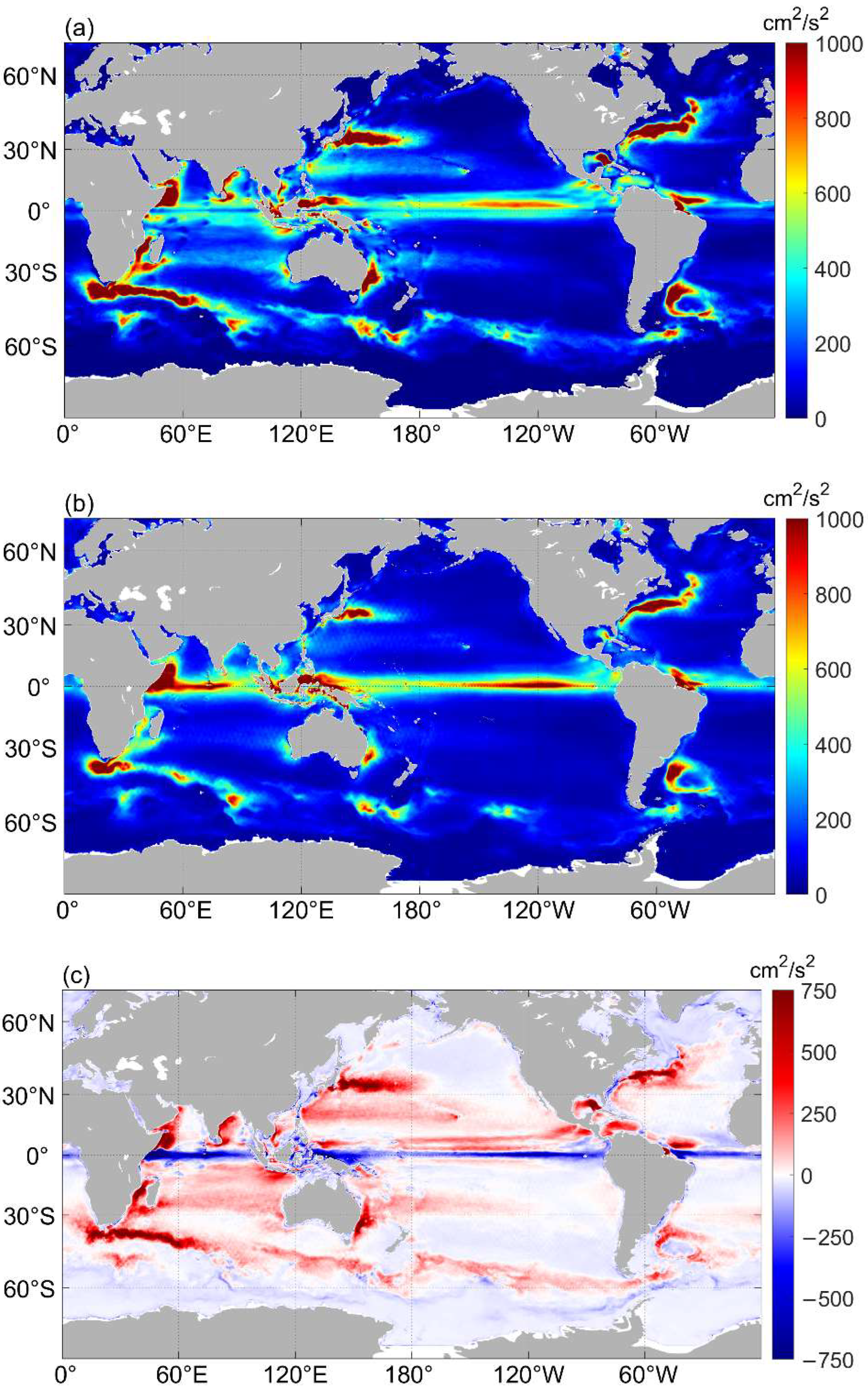
Figure 1a,b show the global distributions of climatological mean EKE and AKE and , respectively. One can see that the high values of above 600 cm2/s2 are mainly distributed in the western boundary current, the Antarctic circumpolar current (ACC), and the equatorial current regions, where maximum values are even higher than 1000 cm2/s2. Mesoscale eddies are frequently active in regions with strong currents due to barotropic and baroclinic instabilities of the background currents, while ageostrophic motions could be enhanced due to active nonlinear eddy–eddy interactions and eddy–current interactions. In addition, ageostrophic forces, such as buoyancy fluxes and wind forcing, are generally large in these areas and induce high ageostrophic energy [40,41,42]. In shallow shelf waters, bottom friction may also contribute to the ageostrophic motions [15,43]. Though high values of and are in close regions, they are dislocated in detail since high ageostrophic motions are prone to appear around mesoscale eddies. have more coverage of high values than indeed.
The difference between and is shown in Figure 1c. The positive values represent stronger geostrophic activities, which are mainly distributed in the western boundary current region and the ACC region, while higher ageostrophic kinetic energy are mainly concentrated in the equatorial region and continental shelf seas, where large winds or bottom friction occurs. The distributions of climatologic LAE and HAE are similar to that of , but is four times greater than (not shown). In other words, low-frequency motions are the dominant components in ageostrophic motions.
2.4. Matching Gridded Data and Normalization
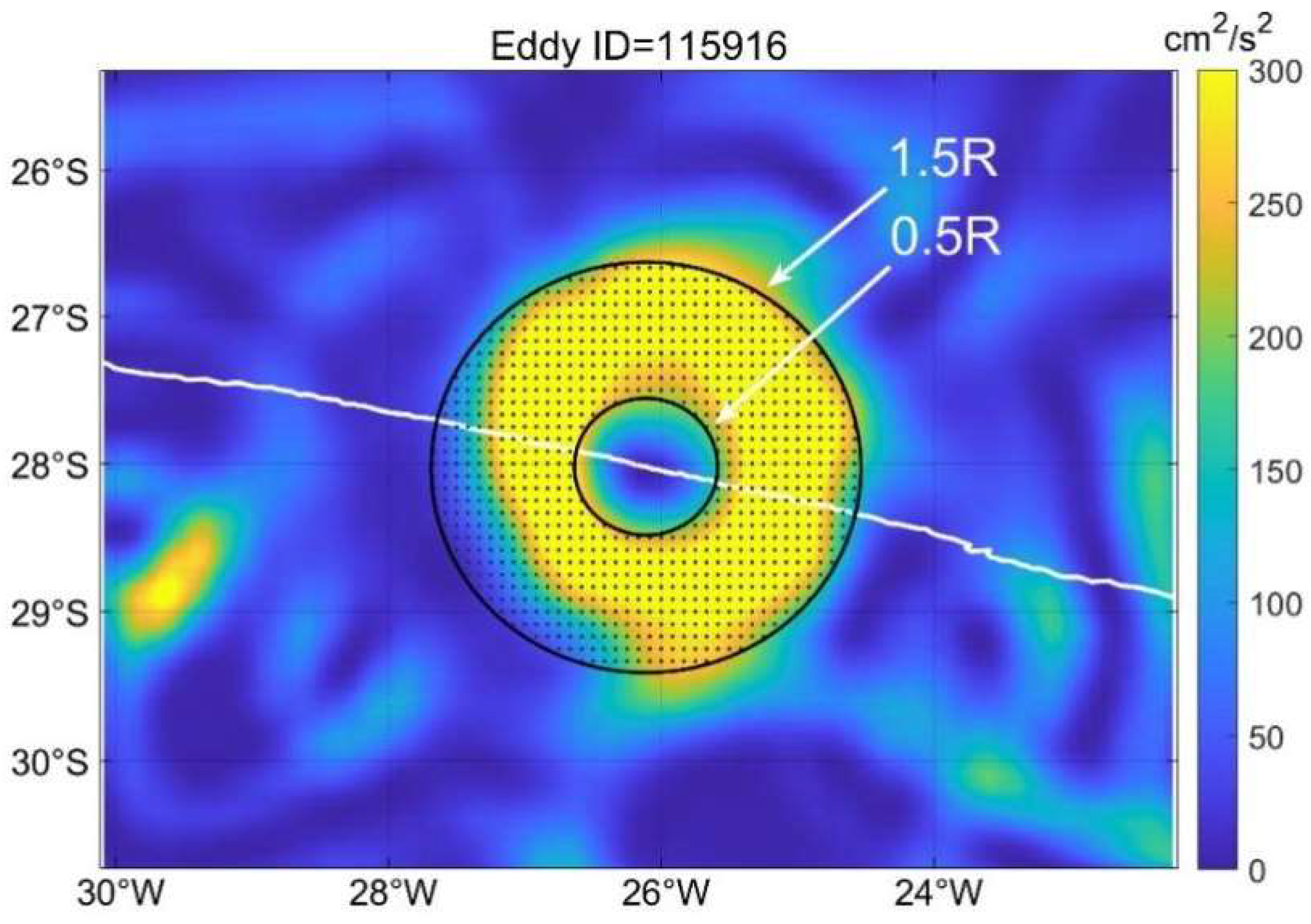
The daily center position and corresponding radius R of the eddies are derived from the eddy-tracking dataset. The area within 0.5–1.5 R around the eddy center is chosen as the main contribution area of the EKE, as in a previous study [14]. The gridded Ega within this area is averaged to represent the EKE of mesoscale eddies at time t, as shown in Figure 2. As a result, Ega(eddy,t) for a certain eddy can be captured along the eddy track on each day t of the eddy life span. In fact, the variation of Ega(eddy,t) here within 0.5–1.5 R is consistent with that derived from the maximum speed of eddies (not shown), although the mean Ega within 0.5–1.5 R is smaller than that from the maximum speed.
The life span of each eddy is then normalized by its total lifespan Tspan, i.e., Te = t/Tspan. Averaging all energy curves along the eddy track in the normalized life span, we could gain the direct mean energy curve Exx (Te) from all eddies, i.e.,
where N is the number of eddy samples, and the subscript xx represents the energy categories, such as ga, ag, alp and ahp.
In order to clarify the portion of energy variation, we normalize the energies on each day of the life cycle Exx(eddy, Te) by its life-mean EKE :
Finally, Exxn(eddy, Te) along the track in the normalized life span for all mesoscale eddies are averaged to obtain the mean curve of Exxn(Te) throughout the eddy life cycle, i.e., . Therefore, the variation curves of EKE Eagn, AKE Eagn, LKE Ealpn, and HKE Eahpn are derived. The mean standard error, std/N1/2, is used to measure the deviation of the mean curves, where std is the standard deviation of the data and N is the number of averaged eddy samples.
3. Results
3.1. Eddy Kinetic Energy Variation during Eddy Life Span
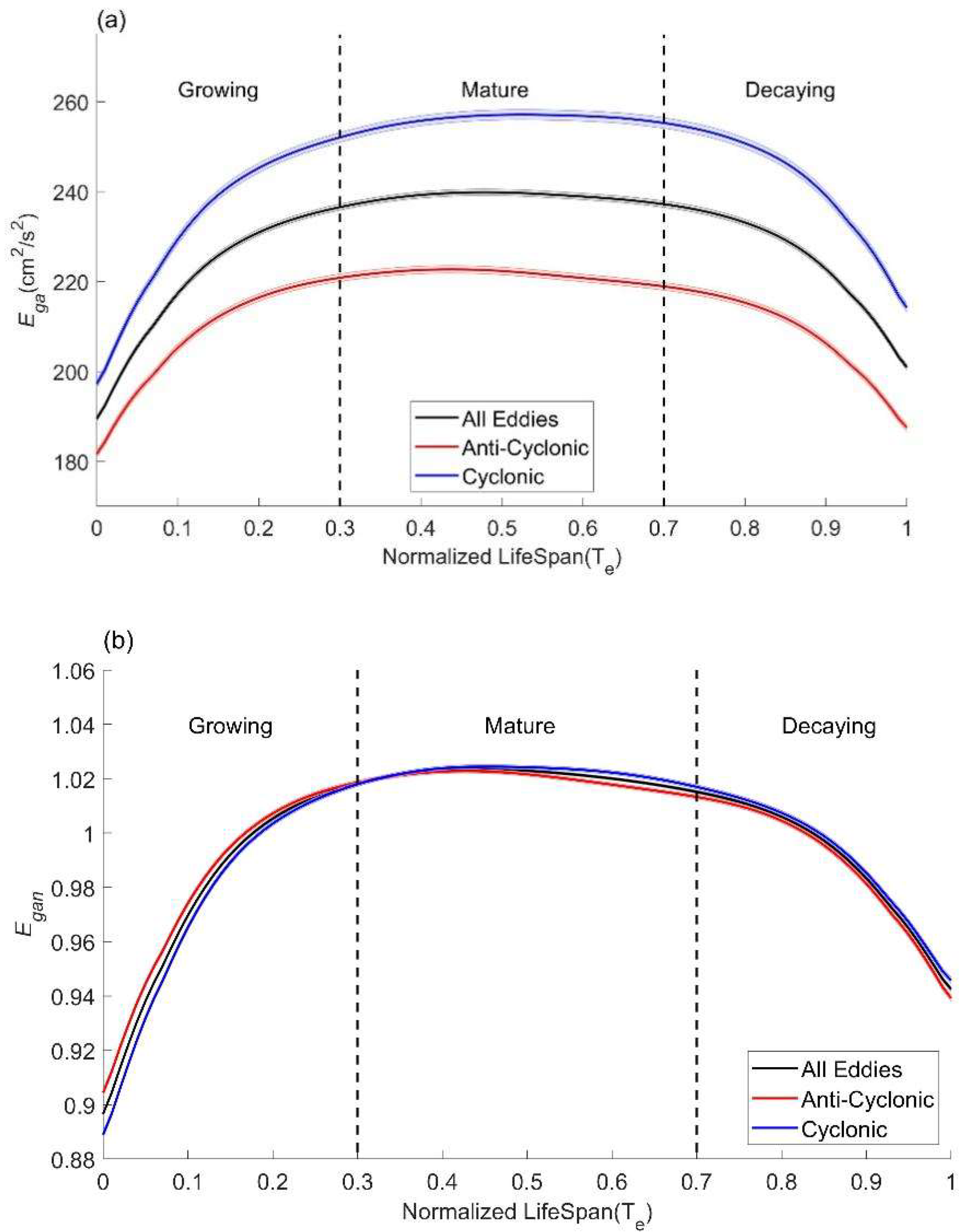
Figure 3a shows the variation of the direct mean EKE Ega for all eddies (black curve), AEs (red curve), and CEs (blue curve) along their tracks during their normalized life span. One can see that the three curves show a similar pattern, i.e., increasing at the beginning, maintaining in the middle, and decreasing at the end. Specifically, Ega for all eddies increases from 190 cm2/s2 at the beginning of the life span to 237 cm2/s2 at 0.3 Te. Subsequently, Ega maintains around 240 cm2/s2 until 0.7 Te and decreases rapidly to 200 cm2/s2 at the end of the life span (black line). The mean Ega over the life span is 229 cm2/s2, lower than 245 cm2/s2 for CEs, and higher than 213 cm2/s2 for AEs.
According to the changing rate of Ega(Te) for total eddies with time, we divide the whole eddy life span into three stages with a critical slope of 0.35 cm2/s2 per 0.01 Te: the growing stage from 0 to 0.3 Te, the mature stage from 0.3 to 0.7 Te, and the decaying stage from 0.7 to 1 Te, as shown in Figure 3a. The energy curves of AEs (red line) and CEs (blue line) have similar patterns to the total one (black line), while the EKE values of CEs are systematically higher than those of AEs, as also observed by Chen and Han [29]. Note that the curves of Ega(Te) are not symmetric. The energy values at the beginning are 5–15 cm2/s2 smaller than that at the end of the eddy life span. The differences between the curves of CEs and AEs in the growing stage are also smaller than that in the decaying stage.
The global mean of the normalized EKE Egan(Te) curve is shown in Figure 3b. One can see that the mean Egan(Te) was 1.02 in the mature stage, while the minimum values are 0.90 and 0.94 at the beginning and the end of the eddy life span, respectively. In contrast to the higher Ega(Te) for CEs in Figure 3a, the normalized Egan(Te) of AEs is generally close to that of CEs, and the Egan(Te) of AEs has larger values in the growing stage. The difference may be attributed to more strong CEs than AEs. The statistics reveal 25.7% of CEs have a larger than 240 cm2/s2, while the ratio is only 23.2% for AEs. In the direct mean of Ega(Te), strong eddies contribute more to the mean value, while the normalized mean curve Egan(Te) reveals the real portion of energy variation over the life span for each eddy. On the other hand, the asymmetry of the curve in the beginning and ending are enhanced in the normalized curve since the eddies are weaker in the growing and decaying stages.
Table 2 lists the energy increments of individual components, in the growing stage and in the decaying stage for all eddies. One can see that = 0.12 and = −0.08, i.e., Egan increases by 12.1% of in the growing stage and decreases by 8% of in the decaying stage.
3.2. Ageostrophic Kinetic Energy Variation during Eddy Life Span
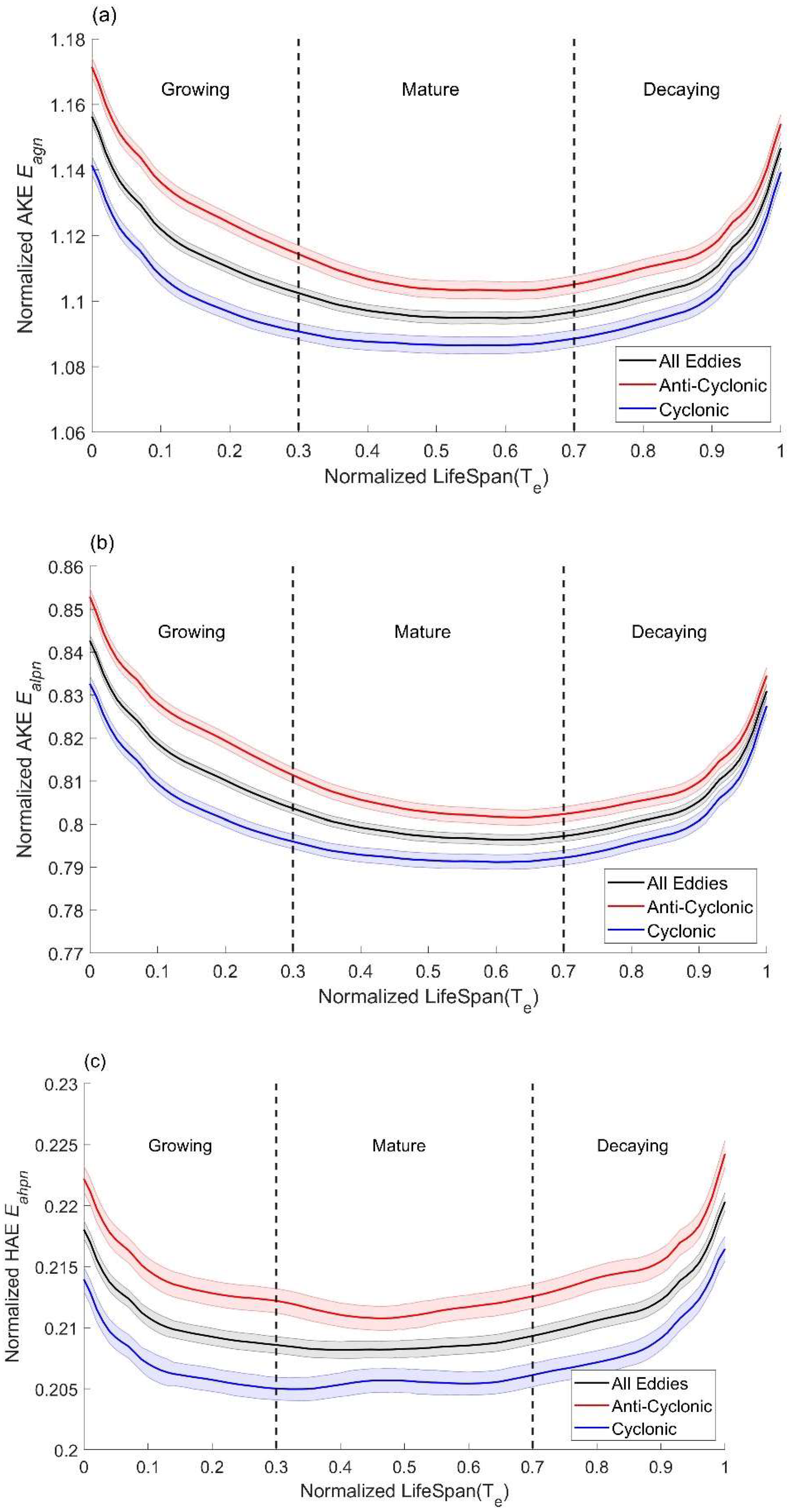
Figure 4a shows the mean curve of the normalized AKE Eagn(Te) during the eddy life span. One can see that the Eagn of total eddies has a maximum value of 1.16 in the growing stage, a minimum value of 1.09 in the mature stage, and 1.15 in the decaying stage. It has an upside-down variation trend compared to the curve of Egan shown in Figure 3b. As listed in Table 2, Eagn decreased by 0.07 in the eddy growing stage and increased by 0.06 in the decaying stage, which accounted for 57% and 75% of |∆Egan| in the two stages, respectively. CEs and AEs both have similar variation trends in the normalized AKE, while the values of AEs are higher than that of CEs, probably due to stronger geostrophic strain in AEs [14].
The mean curves of the normalized LAE Ealpn (>7 d) and the normalized HAE Eahpn (<7 d) during the eddy life span are further shown in Figure 4b,c. One can see that the energy curves of both Ealpn and Eahpn are similar to that of the total ageostrophic energy Eagn shown in Figure 4a. The maximum and minimum values of Ealpn are 0.84, 0.80, and 0.83 in the three stages, accounting for 62% of the values of total ageostrophic energy Eagn. On the other hand, the extreme values of Eahpn for all eddies are only 0.22, 0.21, and 0.22 in the three stages. They are four times lower than those of Ealpn, indicating that Ealpn is the dominant component in Ean.
3.3. Analysis of Coherence of EKE Variation to Low-Frequency Ageostrophic Motions
As shown in Figure 4, the curves of Ealpn and Eahpn are highly coherent with that of Egan during the eddy life span. The correlation coefficient reaches −0.94 and −0.89 with a confidence level of 99% for Ealpn and Eahpn, respectively. This indicates that both low-frequency and high-frequency ageostrophic motions contribute to EKE variation during the eddy life span, while the low-frequency ageostrophic motions are more closely correlated to the EKE variation.
Table 2 lists the ratios of the contribution. One can see that in the growing stage, Ealpn decreases by 0.05 from 0.84 to 0.79, contributing 38% of . On the other hand, Ealpn increases by 0.03 (42% of ) in the decaying stage. On average, the energy provided by the low-frequency ageostrophic motions contributes 40% of the total variation of Egan. For comparison, the contributions of high-frequency ageostrophic motions to the variation of Egan are also listed in Table 2. The ratios are only 8% and 15% in the growing and decaying stages, respectively, 3–5 times lower than the ratio of Ealpn to Egan. The low-frequency ageostrophic motions are a major contributor.
3.4. Barotropic Conversion Rate
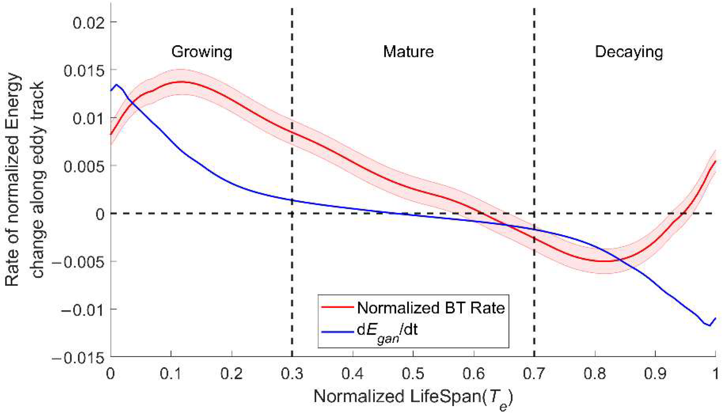
In order to investigate the interactions among eddies and low-frequency ageostrophic motions, we performed energy analysis to quantify the barotropic (BT) conversion rate between the EKE and the LAE. We first integrate the EKE within the range of 0.5–1.5 R and obtain the integrated-EKE (iEKE) curve for each eddy. Then, the integrated-EKE curve for each eddy is normalized by its life-mean EKE , and the global mean of the normalized iEKE curve is obtained, which has similar patterns to the EKE Ega curve (not shown). We calculate the time derivative dEgan/dt of the mean normalized iEKE curve in the eddy life span. The resulted dEgan/dt is shown by the blue curve in Figure 5.
For the eddy energy variation, the total derivative of eddy kinetic energy without external forcing depends on four dynamic terms, i.e., the shear production of the background current (i.e., BT conversion rate), the buoyant production (i.e., BC conversion rate), the viscosity dissipation, and the energy flux divergence [13,44]. In which the BT conversion rate represents the energy transfer from the background current to the eddy geostrophic current. It is calculated as follows [13]:
We calculate the BT rate for data grids first and then select values along the eddy track to calculate the integrated BT rate within the range of 0.5–1.5 R during the eddy life span. Then, the integrated BT rate curve is also normalized by its life-mean EKE for each eddy. Finally, the curves of all global eddies are averaged to obtain the red curve shown in Figure 5. One can see that the normalized BT rate is positive in the eddy growing and mature stage, indicating that the energy transfers from low-frequency motions to eddies, while the BT rate is negative in the decaying stage, where the energy transfers inversely from EKE to LAE.
Comparing the BT rate to the change rate of EKE along the eddy track (dEgan/dt, blue line in Figure 5), one can see that the two rates have the same decreasing trend during the eddy life span and change the sign of variation rate in the mature stage. Their correlation coefficient reaches 0.73 with 99% significance, indicating that the BT rate is the dominant term in the eddy energy variation. The BT rate is generally larger than the EKE variation rate dEgan/dt. In the eddy growing stage, EKE increases with a positive dE/dt as LAE transfers to EKE with a positive BT rate; EKE varies little with |dEgan/dt| less than 1.5 × 10⁻³ as the BT rate decrease rapidly in the mature stage. Then, EKE decreases with a negative rate in the decaying stage, as the BT rate becomes negative. It is clear that low-frequency ageostrophic motions serve as the energy sources for eddy growth and the energy sink for eddy decay. Furthermore, the BT rate was positive between 0 and 0.62 Te, while dEgan/dt becomes negative after 0.47 Te, implying EKE loss possibly probably due to high-frequency ageostrophic motions, viscous dissipation, wind killing, and energy transfer to potential energy [32,45,46]. The positive anomaly after 0.95 Te may be caused by eddy shape deforming or eddy–mean flow interaction at the western boundary [47,48].
4. Discussion
Previous investigators found a high correlation between the high-passed ageostrophic kinetic energy and eddy geostrophic kinetic energy during the eddy life span and proposed the importance of submesoscale processes in eddy kinetic energy variation [14]. In this study, we found close coherence in the EKE variation to low-frequency ageostrophic motions such as slowly varying wind-driven flow and planet waves because of their shared frequency band with mesoscale eddies rather than submesoscale processes.
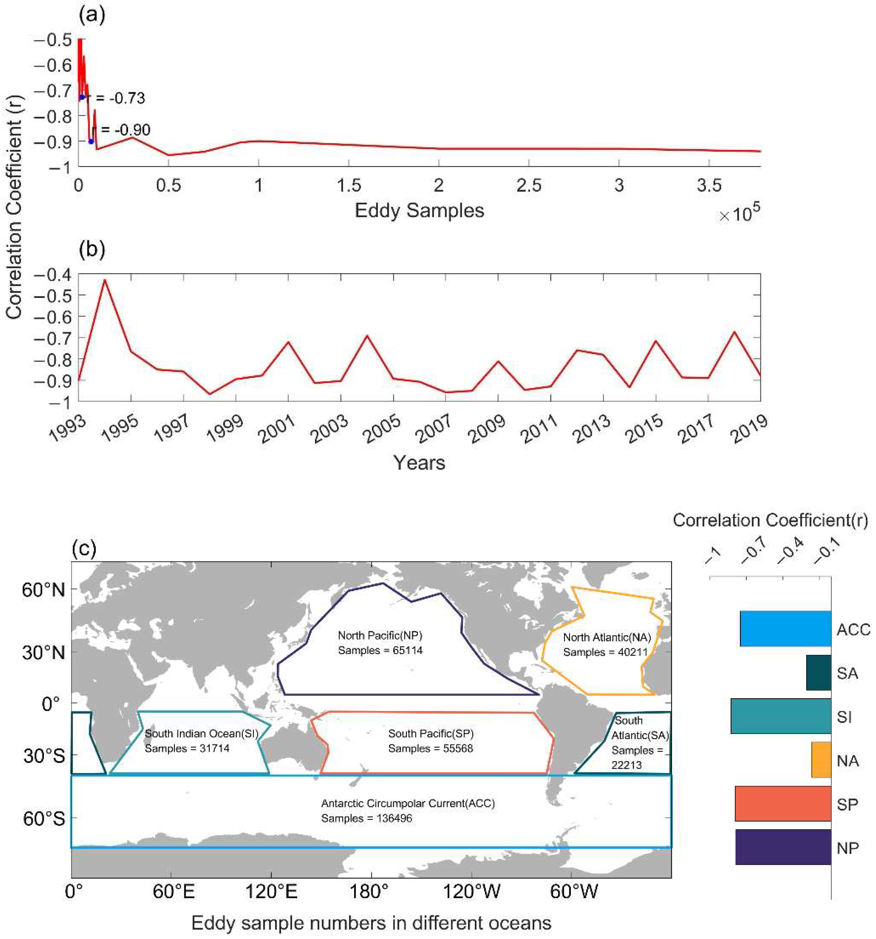
It should be noted that the high coherence of variations of EKE and LAE in this study are a composite result of total eddies in the global ocean. The number of eddy samples N, as well as the locations and occurrence time of eddies, may have an influence on the coherence between EKE and LAE. Figure 6a shows the variation of the correlation coefficient between Egn and Ealpn, marked as r, with different numbers of random eddy samples in the global ocean. One can see that r oscillates around 0 as the number of eddy samples N is less than 2000, increases gradually from about −0.73 at N = 2000 to −0.90 as N reaches 7000, and keeps to a little more than −0.92 with N > 10,000. It indicates that the coherence between the curves of EKE and LAE could be established if there were more than 2000 eddies. We further calculate r between Egn and Ealpn of the eddies in each year. As shown in Figure 6b, r has the largest value of −0.95 in 1998 and then varies between −0.7 and −0.94 with a 2–3 year period in the recent 20 years, which seems to be related to the interannual variability of eddies and background currents influenced by ENSO [23,49,50]. For spatial variability of the coherence shown in Figure 6c, the correlation r between Egn and Ealpn is larger than −0.8 in most oceans except in the Atlantic, probably due to the narrow and asymmetric ocean basin. Mechanisms about the coherence variation need further pursuing.
We find three-stage variations of eddy energy during eddy life for global ocean eddies. In fact, such composite three-stage evolution has been reported for eddies both in the open ocean [2,14,27,29] and in regional seas [26,28,29,51], though the variation rates and the span of each stage may be different in different seas in different years. It should be noted that the three-stage pattern is also the composite result of large amounts of eddies. For a single eddy, the energy curve during its life cycle may be complicated due to various forcing [52,53]. The interaction between eddies, such as merging and splitting, could also cause eddy energy variation during their lives [54,55]. In addition, only eddies with a life cycle of more than 30 days are considered in this study due to data limitations. It will be helpful to comprehensively understand the evolution of mesoscale eddies by separating eddies within different ranges of radius and life span. Furthermore, only sea surface current energy and BT conversion rate are analyzed; the baroclinic instability process and eddy energy conversion to ageostrophic current could be further explored.
5. Conclusions
Using satellite altimetry data and reanalysis current velocity data from 1993 to 2019, this study analyzes the role of low-frequency ageostrophic motions in the variation of eddy kinetic energy during eddy life span in global ocean. The quantitative analysis showed that the Egan curve and the Ealpn curve throughout the eddy life span have a correlation coefficient of −0.94. Low-frequency ageostrophic motion contributes about 38% of the EKE variation in the eddy generation phase and 42% in the decaying phase. Thus, it is the low-frequency ageostrophic motions that are closely coherent with the EKE variation during the eddy life span. In addition, the BT conversion rate analysis confirmed the relationship between the energy transfer between LAE and EKE. Moreover, the EKE decrease in the decaying stage may also be attributed to other processes such as wind work, submesoscale processes, and topography effect.
The new findings in this study may help to improve the understanding of the mechanisms involved in the generation and dissipation of mesoscale eddies and the role of mesoscale eddies in the global ocean energy cascade. Meanwhile, the results in the ocean may also provide a reference for the other geophysical fluid on the Earth, the atmosphere. Different from the same-order geo- and ageostrophic energies in the ocean (Figure 1c), the ageostrophic energy in the atmosphere is weaker than that of geostrophic motion [5,14,56]. Nonetheless, ageostrophic motion is still important in weather-scale processes in the atmosphere and contributes to the enhancement of the geostrophic field [15,57]. The role of ageostrophic motions in the atmospheric energy cascade could be compared to that in the ocean in further studies.
Author Contributions
Z.Z.: data analysis; writing—original draft; L.X.: study design; writing—review and editing. Q.Z.: concepts discussed; writing—review and editing; M.L. (Mingming Li), J.L. and M.L. (Min Li): concepts discussed; suggestions provided. All authors have read and agreed to the published version of the manuscript.
Funding
This research was funded by the National Natural Science Foundation of China (41776034 and 411706025), the Project of Enhancing School with Innovation of Education Department of Guangdong Province (2019KCXTF021), and the Guangdong Province First-Class Discipline Plan (080503032101 and 231420003).
Data Availability Statement
The mesoscale eddy trajectories atlas product META 2.0 DT is distributed by AVISO at: https://www.aviso.altimetry.fr/en/data/products/value-added-products/global-mesoscale-eddy-trajectory-product.html, (accessed on 22 July 2020). The global gridded current velocity can be accessed at: https://resources.marine.copernicus.eu/product-detail/GLOBAL_MULTIYEAR_PHY_001_030/ (accessed on 6 September 2021). The global altimeter satellite gridded geostrophic velocities anomalies are available at: https://resources.marine.copernicus.eu/product-detail/SEALEVEL_GLO_PHY_L4_MY_008_047/ (accessed on 22 July 2020).
Acknowledgments
The authors thank Zhengguang Zhang for discussion and data processing.
Conflicts of Interest
The researchers declare no conflict of interest.
References
- Roemmich, D.; Gilson, J. Eddy Transport of Heat and Thermocline Waters in the North Pacific: A Key to Interannual/Decadal Climate Variability? J. Phys. Oceanogr. 2001, 31, 675–687. [Google Scholar] [CrossRef]
- Chelton, D.B.; Schlax, M.G.; Samelson, R.M. Global observations of nonlinear mesoscale eddies. Prog. Oceanogr. 2011, 91, 167–216. [Google Scholar] [CrossRef]
- Dong, C.; McWilliams, J.C.; Liu, Y.; Chen, D. Global heat and salt transports by eddy movement. Nat. Commun. 2014, 5, 3294. [Google Scholar] [CrossRef] [PubMed] [Green Version]
- Zhang, Z.; Wang, W.; Qiu, B. Oceanic mass transport by mesoscale eddies. Science 2014, 345, 322–324. [Google Scholar] [CrossRef] [PubMed]
- Zhang, Z.; Qiu, B.; Klein, P.; Travis, S. The influence of geostrophic strain on oceanic ageostrophic motion and surface chlorophyll. Nat. Commun. 2019, 10, 2838. [Google Scholar] [CrossRef] [PubMed] [Green Version]
- Adams, D.K.; McGillicuddy, D.J., Jr.; Zamudio, L.; Thurnherr, A.M.; Liang, X.; Rouxel, O.; German, C.R.; Mullineaux, L.S. Surface-generated mesoscale eddies transport deep-sea products from hydrothermal vents. Science 2011, 332, 580–583. [Google Scholar] [CrossRef] [Green Version]
- Hausmann, U.; Czaja, A. The observed signature of mesoscale eddies in sea surface temperature and the associated heat transport. Deep Sea Res. Part I Oceanogr. Res. Pap. 2012, 70, 60–72. [Google Scholar] [CrossRef]
- Kamenkovich, I.; Berloff, P.; Haigh, M.; Sun, L.; Lu, Y. Complexity of Mesoscale Eddy Diffusivity in the Ocean. Geophys. Res. Lett. 2021, 48, e2020GL091719. [Google Scholar] [CrossRef]
- Ferrari, R.; Wunsch, C. Ocean Circulation Kinetic Energy: Reservoirs, Sources, and Sinks. Annu. Rev. Fluid Mech. 2009, 41, 253–282. [Google Scholar] [CrossRef] [Green Version]
- Huang, R.X. Ocean Circulation: Wind-Driven and Thermohaline Processes; Cambridge University Press: Cambridge, UK, 2010; p. 195. [Google Scholar]
- Chen, R.; Flierl, G.R.; Wunsch, C. A Description of Local and Nonlocal Eddy–Mean Flow Interaction in a Global Eddy-Permitting State Estimate. J. Phys. Oceanogr. 2014, 44, 2336–2352. [Google Scholar] [CrossRef] [Green Version]
- Vallis, G.K. Atmospheric and Oceanic Fluid Dynamics; Cambridge University Press: Cambridge, UK, 2017. [Google Scholar]
- Kang, D.; Curchitser, E.N. Energetics of Eddy–Mean Flow Interactions in the Gulf Stream Region. J. Phys. Oceanogr. 2015, 45, 1103–1120. [Google Scholar] [CrossRef]
- Zhang, Z.; Qiu, B. Evolution of Submesoscale Ageostrophic Motions Through the Life Cycle of Oceanic Mesoscale Eddies. Geophys. Res. Lett. 2018, 45, 11847–11855. [Google Scholar] [CrossRef] [Green Version]
- McWilliams, J.C. Submesoscale currents in the ocean. Proc. Math. Phys. Eng. Sci. 2016, 472, 20160117. [Google Scholar] [CrossRef] [PubMed]
- Xu, C.; Shang, X.-D.; Huang, R.X. Estimate of eddy energy generation/dissipation rate in the world ocean from altimetry data. Ocean Dyn. 2011, 61, 525–541. [Google Scholar] [CrossRef]
- Yang, Z.; Zhai, X.; Marshall, D.P.; Wang, G. An Idealized Model Study of Eddy Energetics in the Western Boundary “Graveyard”. J. Phys. Oceanogr. 2021, 51, 1265–1282. [Google Scholar] [CrossRef]
- Xu, C.; Zhai, X.; Shang, X.-D. Work done by atmospheric winds on mesoscale ocean eddies. Geophys. Res. Lett. 2016, 43, 12174–112180. [Google Scholar] [CrossRef] [Green Version]
- Chelton, D.B.; Gaube, P.; Schlax, M.G.; Early, J.J.; Samelson, R.M. The influence of nonlinear mesoscale eddies on near-surface oceanic chlorophyll. Science 2011, 334, 328–332. [Google Scholar] [CrossRef]
- Chen, G.; Wang, D.; Hou, Y. The features and interannual variability mechanism of mesoscale eddies in the Bay of Bengal. Cont. Shelf Res. 2012, 47, 178–185. [Google Scholar] [CrossRef]
- Zhai, X.; Marshall, D.P. Vertical Eddy Energy Fluxes in the North Atlantic Subtropical and Subpolar Gyres. J. Phys. Oceanogr. 2013, 43, 95–103. [Google Scholar] [CrossRef]
- Trott, C.B.; Subrahmanyam, B.; Chaigneau, A.; Delcroix, T. Eddy Tracking in the Northwestern Indian Ocean During Southwest Monsoon Regimes. Geophys. Res. Lett. 2018, 45, 6594–6603. [Google Scholar] [CrossRef]
- Zheng, S.; Feng, M.; Du, Y.; Meng, X.; Yu, W. Interannual Variability of Eddy Kinetic Energy in the Subtropical Southeast Indian Ocean Associated With the El Niño-Southern Oscillation. J. Geophys. Res. Ocean. 2018, 123, 1048–1061. [Google Scholar] [CrossRef]
- Li, J.; Roughan, M.; Kerry, C. Dynamics of Interannual Eddy Kinetic Energy Modulations in a Western Boundary Current. Geophys. Res. Lett. 2021, 48, e2021GL094115. [Google Scholar] [CrossRef]
- Chen, S.; Qiu, B. Variability of the Kuroshio Extension Jet, Recirculation Gyre, and Mesoscale Eddies on Decadal Time Scales. J. Phys. Oceanogr. 2005, 35, 2090–2103. [Google Scholar]
- Liu, Y.; Dong, C.; Guan, Y.; Chen, D.; McWilliams, J.; Nencioli, F. Eddy analysis in the subtropical zonal band of the North Pacific Ocean. Deep Sea Res. Part I Oceanogr. Res. Pap. 2012, 68, 54–67. [Google Scholar] [CrossRef]
- Chelton, D.B.; Schlax, M.G.; Samelson, R.M. Randomness, Symmetry, and Scaling of Mesoscale Eddy Life Cycles. J. Phys. Oceanogr. 2014, 44, 1012–1029. [Google Scholar]
- Ji, J.; Dong, C.; Zhang, B.; Liu, Y.; Zou, B.; King, G.P.; Xu, G.; Chen, D. Oceanic Eddy Characteristics and Generation Mechanisms in the Kuroshio Extension Region. J. Geophys. Res. Ocean. 2018, 123, 8548–8567. [Google Scholar] [CrossRef]
- Chen, G.; Han, G. Contrasting Short-Lived With Long-Lived Mesoscale Eddies in the Global Ocean. J. Geophys. Res. Ocean. 2019, 124, 3149–3167. [Google Scholar] [CrossRef]
- Huang, R.; Xie, L.; Zheng, Q.; Li, M.; Bai, P.; Tan, K. Statistical analysis of mesoscale eddy propagation velocity in the South China Sea deep basin. Acta Oceanol. Sin. 2021, 39, 91–102. [Google Scholar] [CrossRef]
- Zhai, X.; Johnson, H.L.; Marshall, D.P. Significant sink of ocean-eddy energy near western boundaries. Nat. Geosci. 2010, 3, 608–612. [Google Scholar] [CrossRef]
- Kang, D.; Curchitser, E.N.; Rosati, A. Seasonal Variability of the Gulf Stream Kinetic Energy. J. Phys. Oceanogr. 2016, 46, 1189–1207. [Google Scholar] [CrossRef]
- Macdonald, H.S.; Roughan, M.; Baird, M.E.; Wilkin, J. The formation of a cold-core eddy in the East Australian Current. Cont. Shelf Res. 2016, 114, 72–84. [Google Scholar] [CrossRef]
- Geng, W.; Xie, Q.; Chen, G.; Zu, T.; Wang, D. Numerical study on the eddy–mean flow interaction between a cyclonic eddy and Kuroshio. J. Oceanogr. 2016, 72, 727–745. [Google Scholar] [CrossRef]
- Yang, H.; Wu, L.; Liu, H.; Yu, Y. Eddy energy sources and sinks in the South China Sea. J. Geophys. Res. Ocean. 2013, 118, 4716–4726. [Google Scholar] [CrossRef]
- Pujol, M.-I.; Faugère, Y.; Taburet, G.; Dupuy, S.; Pelloquin, C.; Ablain, M.; Picot, N. DUACS DT2014: The new multi-mission altimeter data set reprocessed over 20 years. Ocean Sci. 2016, 12, 1067–1090. [Google Scholar] [CrossRef] [Green Version]
- Schlax, M.G.; Chelton, D.B. The “Growing Method” of Eddy Identification and Tracking in Two and Three Dimensions; College of Earth, Ocean and Atmospheric Sciences, Oregon State University: Corvallis, OR, USA, 2016; pp. 1–8. Available online: https://www.aviso.altimetry.fr/fileadmin/documents/data/products/value-added/Schlax_Chelton_2016.pdf (accessed on 14 December 2021).
- Thomas, L.N.; Tandon, A.; Mahadevan, A. Submesoscale processes and dynamics. In Ocean Modeling in an Eddying Regime; Geophysical Monograph Series; Wiley-Blackwell Publishing: Hoboken, NJ, USA, 2008; pp. 17–38. [Google Scholar]
- Lévy, M.; Ferrari, R.; Franks, P.J.S.; Martin, A.P.; Rivière, P. Bringing physics to life at the submesoscale. Geophys. Res. Lett. 2012, 39. [Google Scholar] [CrossRef] [Green Version]
- Colas, F.; Capet, X.; McWilliams, J.C.; Li, Z. Mesoscale Eddy Buoyancy Flux and Eddy-Induced Circulation in Eastern Boundary Currents. J. Phys. Oceanogr. 2013, 43, 1073–1095. [Google Scholar] [CrossRef]
- Stammer, D.; Böning, C.; Dieterich, C. The role of variable wind forcing in generating eddy energy in the North Atlantic. Prog. Oceanogr. 2001, 48, 289–311. [Google Scholar] [CrossRef] [Green Version]
- Hogg, A.M.; Meredith, M.P.; Chambers, D.P.; Abrahamsen, E.P.; Hughes, C.W.; Morrison, A.K. Recent trends in the Southern Ocean eddy field. J. Geophys. Res. Ocean. 2015, 120, 257–267. [Google Scholar] [CrossRef] [Green Version]
- Semtner, A.J.; Mintz, Y. Numerical Simulation of the Gulf Stream and Mid-Ocean Eddies. J. Phys. Oceanogr. 1977, 7, 208–230. [Google Scholar] [CrossRef] [Green Version]
- Kundu, P.K.; Cohen, I.M. Fluid Mechanics; Elsevier Science: Amsterdam, The Netherlands, 2010. [Google Scholar]
- Rai, S.; Hecht, M.; Maltrud, M.; Aluie, H. Scale of oceanic eddy killing by wind from global satellite observations. Sci. Adv. 2021, 7, eabf4920. [Google Scholar] [CrossRef]
- Yang, Q.; Nikurashin, M.; Sasaki, H.; Sun, H.; Tian, J. Dissipation of mesoscale eddies and its contribution to mixing in the northern South China Sea. Sci. Rep. 2019, 9, 556. [Google Scholar] [CrossRef] [PubMed] [Green Version]
- Jan, S.; Mensah, V.; Andres, M.; Chang, M.H.; Yang, Y.J. Eddy-Kuroshio Interactions: Local and Remote Effects. J. Geophys. Res. Ocean. 2017, 122, 9744–9764. [Google Scholar] [CrossRef] [Green Version]
- Chern, C.-S.; Wang, J. Interactions of Mesoscale Eddy and Western Boundary Current: A Reduced-Gravity Numerical Model Study. J. Oceanogr. 2005, 61, 271–282. [Google Scholar] [CrossRef]
- Kuo, Y.-C.; Tseng, Y.-H. Influence of anomalous low-level circulation on the Kuroshio in the Luzon Strait during ENSO. Ocean Model. 2021, 159, 101759. [Google Scholar] [CrossRef]
- Langlais, C.E.; Rintoul, S.R.; Zika, J.D. Sensitivity of Antarctic Circumpolar Current Transport and Eddy Activity to Wind Patterns in the Southern Ocean. J. Phys. Oceanogr. 2015, 45, 1051–1067. [Google Scholar] [CrossRef] [Green Version]
- Zhang, N.; Liu, G.; Liu, Q.; Zheng, S.; Perrie, W. Spatiotemporal Variations of Mesoscale Eddies in the Southeast Indian Ocean. J. Geophys. Res. Ocean. 2020, 125, e2019JC015712. [Google Scholar] [CrossRef]
- Ayouche, A.; De Marez, C.; Morvan, M.; L’Hegaret, P.; Carton, X.; Le Vu, B.; Stegner, A. Structure and Dynamics of the Ras al Hadd Oceanic Dipole in the Arabian Sea. Oceans 2021, 2, 105–125. [Google Scholar] [CrossRef]
- Gnevyshev, V.G.; Malysheva, A.A.; Belonenko, T.V.; Koldunov, A.V. On Agulhas eddies and Rossby waves travelling by forcing effects. Russ. J. Earth Sci. 2021, 21, 3. [Google Scholar] [CrossRef]
- Laxenaire, R.; Speich, S.; Blanke, B.; Chaigneau, A.; Pegliasco, C.; Stegner, A. Anticyclonic Eddies Connecting the Western Boundaries of Indian and Atlantic Oceans. J. Geophys. Res. Ocean. 2018, 123, 7651–7677. [Google Scholar] [CrossRef]
- Keppler, L.; Cravatte, S.; Chaigneau, A.; Pegliasco, C.; Gourdeau, L.; Singh, A. Observed Characteristics and Vertical Structure of Mesoscale Eddies in the Southwest Tropical Pacific. J. Geophys. Res. Ocean. 2018, 123, 2731–2756. [Google Scholar] [CrossRef] [Green Version]
- Errico, R.M. The Strong Effects of Non-Quasigeostrophic Dynamic Processes on Atmospheric Energy Spectra. J. Atmos. Sci. 1982, 39, 961–968. [Google Scholar]
- Straub, D.N.; Bartello, P.; Ngan, K. Dissipation of Synoptic-Scale Flow by Small-Scale Turbulence. J. Atmos. Sci. 2008, 65, 766–791. [Google Scholar]
Figure 1.
Global distributions of climatological kinetic energy. (a) Eddy geostrophic kinetic energy , (b) ageostrophic kinetic energy , (c) differences between and .
Figure 1.
Global distributions of climatological kinetic energy. (a) Eddy geostrophic kinetic energy , (b) ageostrophic kinetic energy , (c) differences between and .

Figure 2.
Matching gridded data along eddy track. The background image shows the EKE field, the white curve represents the eddy trajectory, the black circles give the range of the eddy 0.5–1.5 R, and the scatters between the two concentric circles represent the data points used in the energy calculation for each eddy.

Figure 3.
Curves of global mean eddy kinetic energy along the eddy track throughout the eddy life span. (a) EKE Ega, (b) Normalized EKE Egan. Black curves represent the energy curves for total eddies. Red and blue curves represent the energy curves for AEs and CEs, respectively. Shadows around the energy curves represent the mean standard error.

Figure 4.
Variation curves of global mean ageostrophic kinetic energy along the eddy track throughout the eddy life span. (a) Normalized AKE Eagn, (b) normalized LAE Ealpn (with period > 7 d), and (c) normalized HAE Eahpn (with period < 7 d). Black curves represent the energy curves for total eddies. Red and blue curves represent the energy curves for AEs and CEs, respectively. Shadows around the energy curves represent the mean standard error.

Figure 5.
Time derivative of normalized iEKE (blue line) and normalized barotropic conversion rate (BTn) (red line) throughout the eddy life span. Shadows around the BTn curves represent the mean standard error.
Figure 5.
Time derivative of normalized iEKE (blue line) and normalized barotropic conversion rate (BTn) (red line) throughout the eddy life span. Shadows around the BTn curves represent the mean standard error.

Figure 6.
Variation of correlation coefficient between Egan and Ealpn curves with (a) eddy samples, (b) eddy occurrence years, and (c) ocean basins.
Figure 6.
Variation of correlation coefficient between Egan and Ealpn curves with (a) eddy samples, (b) eddy occurrence years, and (c) ocean basins.


Table 1.
The numbers, radius, and lifespan of mesoscale eddies in the global ocean.
| All | AEs | CEs | |
|---|---|---|---|
| Eddy number | 378,513 | 185,937 | 192,577 |
| Eddy radius (km) median (mean ± std) | 74.20 (82.33 ± 35.93) | 74.95 (83.13 ± 36.23) | 73.45 (81.53 ± 35.60) |
| Eddy lifespan (day) median (mean ± std) | 51.00 (73.38 ± 66.40) | 51.00 (74.43 ± 69.62) | 51.00 (72.60 ± 63.33) |
Table 2.
Increments of Egn, Ean, Ealpn, and Eahpn and contributions to Egn in the growing and decaying stages.
Table 2.
Increments of Egn, Ean, Ealpn, and Eahpn and contributions to Egn in the growing and decaying stages.
| Egn | Ean | Ealpn | Eahpn | |
|---|---|---|---|---|
| Growing stage | 0.12 (100%) | −0.07 (57%) | −0.05 (38%) | −0.01 (8%) |
| Decaying stage | −0.08 (100%) | 0.06 (75%) | 0.03 (42%) | 0.01 (15%) |
Publisher’s Note: MDPI stays neutral with regard to jurisdictional claims in published maps and institutional affiliations. |
© 2022 by the authors. Licensee MDPI, Basel, Switzerland. This article is an open access article distributed under the terms and conditions of the Creative Commons Attribution (CC BY) license (https://creativecommons.org/licenses/by/4.0/).
Share and Cite
MDPI and ACS Style
Zhang, Z.; Xie, L.; Zheng, Q.; Li, M.; Li, J.; Li, M. Coherence of Eddy Kinetic Energy Variation during Eddy Life Span to Low-Frequency Ageostrophic Energy. Remote Sens. 2022, 14, 3793. https://doi.org/10.3390/rs14153793
AMA Style
Zhang Z, Xie L, Zheng Q, Li M, Li J, Li M. Coherence of Eddy Kinetic Energy Variation during Eddy Life Span to Low-Frequency Ageostrophic Energy. Remote Sensing. 2022; 14(15):3793. https://doi.org/10.3390/rs14153793
Chicago/Turabian StyleZhang, Zhisheng, Lingling Xie, Quanan Zheng, Mingming Li, Junyi Li, and Min Li. 2022. "Coherence of Eddy Kinetic Energy Variation during Eddy Life Span to Low-Frequency Ageostrophic Energy" Remote Sensing 14, no. 15: 3793. https://doi.org/10.3390/rs14153793
Note that from the first issue of 2016, this journal uses article numbers instead of page numbers. See further details here.