
Evaluation of CYGNSS Observations for Snow Properties, a Case Study in Tibetan Plateau, China
by
 , ,
, ,
Wenxiao Ma
1,2,† ,
,
Lingyong Huang
3,4,5,†,
Xuerui Wu
6,*,
Shuanggen Jin
1,7,
Weihua Bai
2,3,4,5 and
Xuanran Li
6 1
Shanghai Astronomical Observatory, Chinese Academy of Sciences, Shanghai 200030, China
2
School of Astronomy and Space Science, University of Chinese Academy of Sciences, Beijing 100049, China
3
National Space Science Center, Chinese Academy of Sciences (NSSC/CAS), Beijing 100190, China
4
Beijing Key Laboratory of Space Environment Exploration, Chinese Academy of Sciences, Beijing 100190, China
5
Key Laboratory of Science and Technology on Space Environment Situational Awareness, Chinese Academy of Sciences (CAS), Beijing 100190, China
6
School of Resources, Environment and Architectural Engineering, Chifeng University, Chifeng 024000, China
7
School of Surveying and Land Information Engineering, Henan Polytechnic University, Jiaozuo 454000, China
*
Author to whom correspondence should be addressed.
†
These authors contributed equally to this work.
Remote Sens. 2022, 14(15), 3772; https://doi.org/10.3390/rs14153772
Submission received: 21 June 2022
/
Revised: 30 July 2022
/
Accepted: 1 August 2022
/
Published: 5 August 2022
(This article belongs to the Special Issue Space-Geodetic Techniques)
Abstract
:Snow plays an important role in the water cycle and global climate change, and the accurate monitoring of changes in snow depth is an important task. However, monitoring snow properties is still challenging and unclear, particularly in the Tibetan Plateau, which has rough land and uneven terrain. The traditional monitoring methods have some limitations in monitoring snow depth changes, and the Global Navigation Satellite System-Reflectometry (GNSS-R) provides a new opportunity for snow monitoring. This paper employed data from the Cyclone Global Navigation Satellite System (CYGNSS) to discover the effect of snow properties. Firstly, the observations of CYGNSS were used to find the sensitive to snow properties, and the relationships between signal to noise ratio (SNR), leading edge slope (LES), surface reflectivity (SR), and snow depth were studied and analyzed, respectively. It is found that the correlation between the first two parameters and snow depth is poor, while SR can indicate the changes in snow depth, and is proposed as an indicator of SR change, namely, surface reflectivity–difference ratio factor (SR–DR factor). Furthermore, the long-time series data in the Tibetan Plateau (2018–2019) are used to analyze its effects on the time series of the SR–DR factor, while the influences of the soil freeze/thaw (F/T) process and soil moisture are excluded during the analysis. The results indicate that the SR–DR factor can be a good indicator and discriminator for snow depth. Our work shows that space-borne GNSS-R has the potential for the monitoring of snow properties.
1. Introduction
One of the fundamental components of the water cycle and global energy is the change in snow, which is of great importance for regional climate change, water use, and natural disaster monitoring [1]. The Tibetan Plateau is a sensitive area, and an ecologically fragile zone at risk of climate change, due to its harsh climate and environment, fragile ecology, and frequent snow disasters. It is the region with the highest average elevation in the world. The Tibetan Plateaus is rich in glaciers, snow, and underground ice resources [2], including the headwaters of many rivers in China, and snowmelt water is an important supplementary source of rivers. In the last few years, due to the climate change, the melting of snow and ice on the Tibetan Plateau has accelerated, and the accumulated total amount of snow is also decreasing. The snow on the Tibetan Plateau has an influence not only on the climate of the Chinese mainland, but also on the water circulation and climate systems of the East Asian region. Therefore, the research on snowpack in this area is of great hydrological and climatic importance [3,4]. The Tibetan Plateau is one of the main snow distribution areas in China, and is also an important pastoral area in China. The development of local agriculture and animal husbandry is also closely related to the change in snow cover. As a result, the study of snow cover on the Tibetan Plateau is of great significance for the sustainable development of the regional ecological environment, and agriculture and animal husbandry [5,6,7].
The Tibetan Plateau is a rough land, and has uneven terrain with an average altitude of more than 4000 m. The ground observation stations are rare with the uneven spatial distribution, and the observation time is discontinuous, which cannot meet the needs of research on large-scale snow distribution characteristics [8].
Satellite observations are an effective way to monitor snow cover. Space-borne optical passive sensors provide useful information for monitoring snow cover, but cannot work in high altitude and cloudy areas, due to the limitation of cloud cover [9,10]. Passive microwave remote sensing data are one of the main means of monitoring snow changes, as this method can penetrate through the porous soil layer, cloud, fog, and so on. It can penetrate a certain depth of surface to obtain information on the surface physical parameters. Therefore, microwave remote sensing is the best technology to obtain regional snow depth and snow water equivalent monitoring [11,12,13].
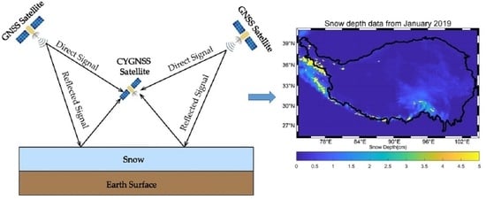
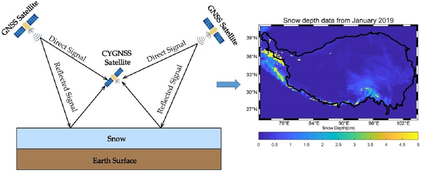
Global Navigation Satellite System-Reflectometry (GNSS-R), using the reflected signals from navigation satellites, was used for remote sensing in recent years [14,15,16]. This method mainly works in the L-band, with strong penetrability, so it is essentially a microwave remote sensing technology. It has the advantages of low cost, low power consumption, and high spatial and temporal resolution, due to the continuous use of navigation satellite signals as a signal source, which does not require the development of a special transmitter. It is a useful supplement to the traditional polar orbit satellites [17].
In 2004 and 2014, the United Kingdom Disaster Monitoring Constellation (UK-DMC) and Techdemosat-1 (TDS-1) test satellites were launched for GNSS-R remote sensing research [18]. In December 2016, the Cyclone Global Navigation Satellite System (CYGNSS) was launched by the National Aeronautics and Space Administration (NASA). The main scientific goal of the system is to measure the ocean surface wind field information during tropical storms and hurricanes [19]. It also provides an important opportunity for the study of land surface parameters, such as soil moisture, vegetation, flood inundation, and wetland monitoring [20,21,22,23]. To the best of our knowledge, there is no reported research on snow cover using CYGNSS data. In this study, the CYGNSS data in the Tibetan Plateau from 1 January 2018 to 31 December 2019 are selected for snow cover analysis. This provides a new method for expanding the research field of satellite-borne CYGNSS, and provides a unique remote sensing method for the study of snow characteristics on the Tibetan Plateau. With the advantages of CYGNSS, using it in the remote sensing of the surface snow depth will improve the temporal resolution of snow depth data, and reduce the effects of background brightness temperature and radio frequency interference (RFI).
2. Method
2.1. Data Description
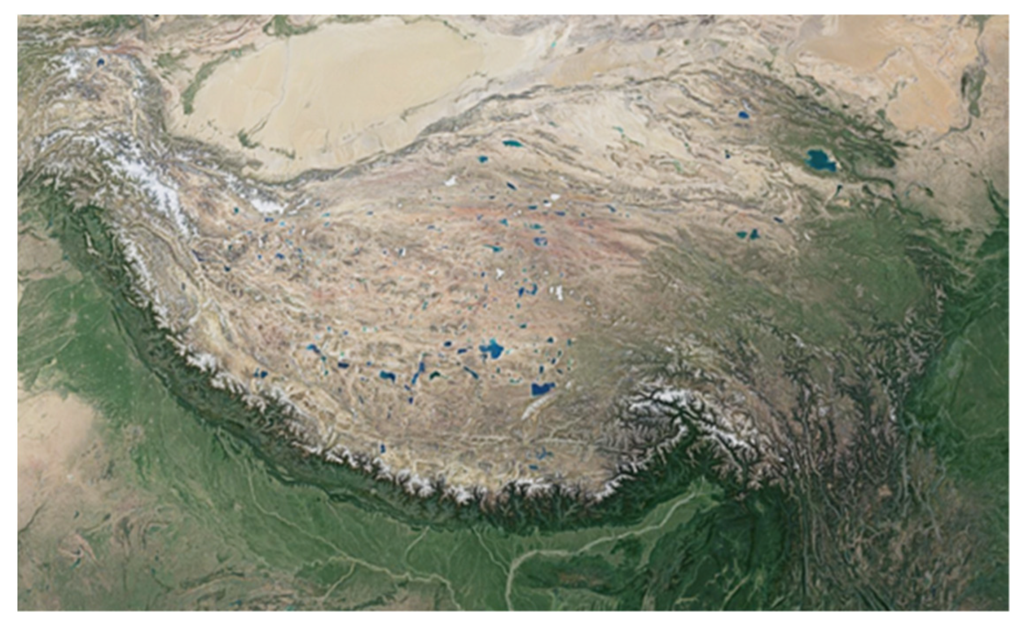
The Tibetan Plateau is the highest plateau in the world, located between 26°N to 39°47′N latitude and 73°19′E to 104°47′E longitude. The topography is complex, and it has large altitude differences in various regions (Figure 1). The average annual temperature decreases from 20 °C in the southeast to below −6 °C in the northwest. In this study, we employed five public datasets to investigate the potential of CYGNSS for the study of snow cover on the Tibetan Plateau: (1) CYGNSS Level-1 (L1) data [24], (2) the Terra and Aqua combined Moderate Resolution Imaging Spectroradiometer (MODIS) Land Cover Climate Modeling Grid (CMG) (MCD12C1) version 6 data (0.05 °C) [25], (3) long-time series dataset of snow depth in China (1979–2019) [26], (4) Soil Moisture Active and Passive (SMAP) L3 radiometer global daily 36 km EASE-grid soil moisture, version 7 [27], (5) European Centre for Medium-Range Weather Forecasts Reanalysis v5 (ERA5) soil temperature data [28].
2.1.1. CYGNSS Data
CYGNSS was successfully launched in December 2016. Eight small satellites carrying GNSS reflection signal receivers make up its constellation. Each CYGNSS satellite is equipped with four delay-Doppler map instruments (DDMI), and each DDMI includes two left-hand circularly polarized (LHCP) antenna and one right-hand circularly polarized (RHCP) antenna. The LHCP antenna receives GNSS signals from specular and scattering points on the Earth’s surface. The RHCP antenna receives GNSS signals directly, to calculate its position and velocity. Each CYGNSS satellite can measure and observe reflections in four directions simultaneously, which means that the CYGNSS system can obtain data from 32 reflection points [29]. The delay-Doppler mapping (DDM) obtained by the receiver is a function of the surface medium, antenna gain, distance, statistical properties, and scattering geometry. The CYGNSS data used in this study were from level 1, version 2.1.
At present, most studies consider that the receiver primarily collects the coherent scattered energy in the first Fresnel region. When only the coherent energy is considered, we can calculate the DDM based on the Friis transmission formula and the Fresnel reflection coefficient of an equivalent smooth surface [30].
- : The transmitted power of GNSS satellite;
- : The GNSS satellite antenna gain at specular point direction;
- : The receiver antenna gain;
- : The GNSS equivalent isotopically radiated power (EIRP);
- : The wavelength;
- and : The distance between the receiver and the specular point and the distance between the transmitter and the specular point, respectively.
According to Equation (1), the reflectivity can be expressed as:
where is the surface rms height, which can characterize the surface roughness, is the incidence angle and the dielectric constant of the geophysical parameters. Surface reflectivity (SR) is usually a small positive value, which is converted to decibel for visualization and data analysis according to Equation (3). Table 1 shows the main parameters for the L1 data used in this study.
It is worth noting that the treatment of the coherent and incoherent scattering is an open issue when dealing with the CYGNSS data [31]. When using CYGNSS data for soil moisture retrieval, the coherent energy comes primarily from specular reflections of water inland within the GNSS-R footprint, which leads to the increase in DDM peak value. The peak energy of the coherent part is many times greater than that in the non-coherent portion. The satellite-based GNSS-R receiver mainly receives coherent scattered signals from the first Fresnel zone around the specular reflection point [32]. In fact, the signals received by GNSS-R receivers, in most cases, contain signals from both coherent and incoherent scattered fields, due to variations in surface roughness. Most of the currently available studies on satellite-based GNSS-R remote sensing of surface soil moisture simplify the scattering mechanism of the L-band on the actual surface, assuming that only coherent scattering occurs on the terrestrial surface, and incoherent scattering is ignored [31]. We removed data with SNRdB less than 2 dB and CYGNSS antenna gain of less than 0 dB. The elevation angle of the specular points is less than 65°.
2.1.2. IGBP Land Cover Classification
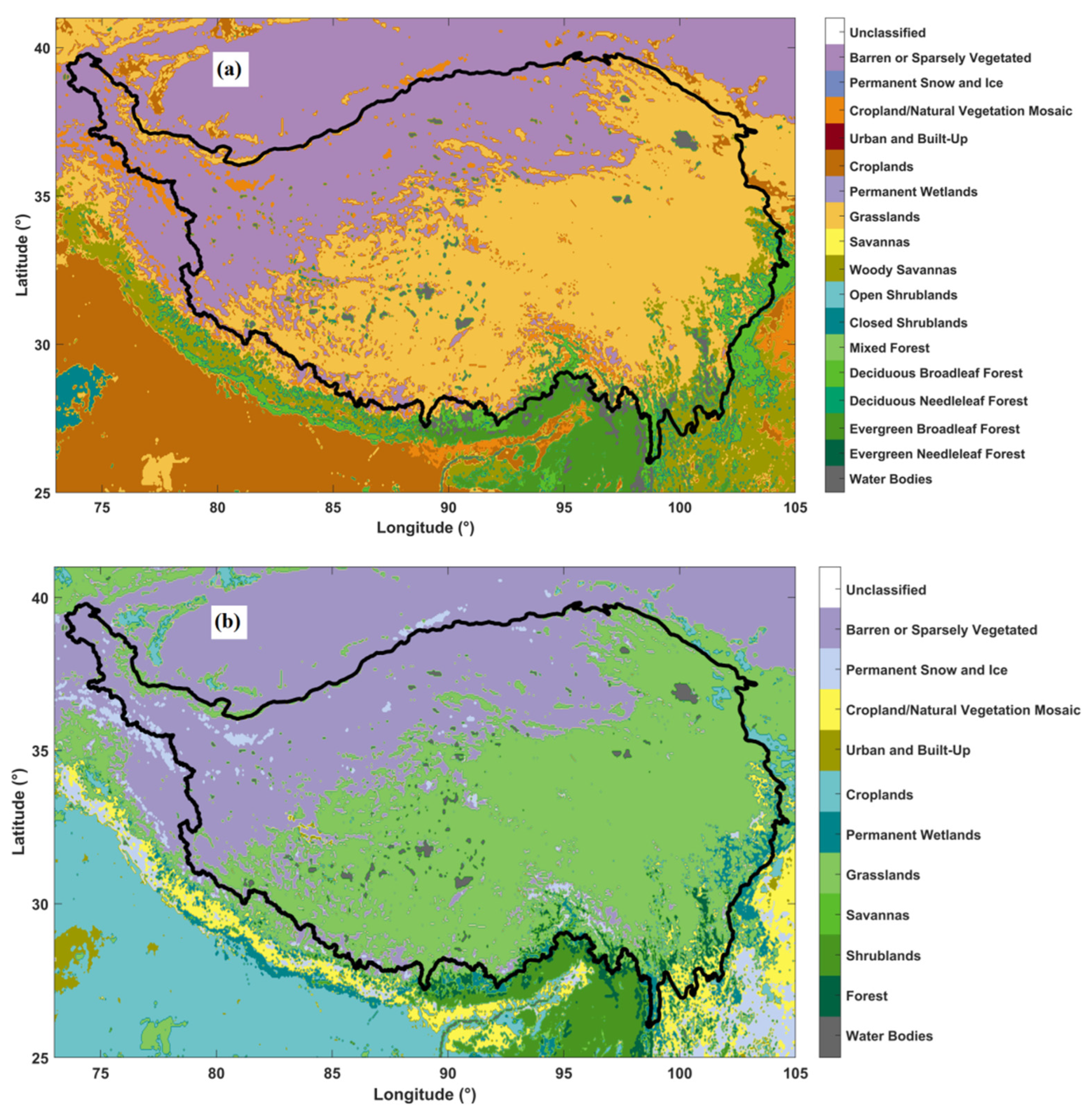
The land surface scattering process is complex. In addition to the influence of surface roughness, the surface scattering signals received directly by GNSS-R receivers are also impacted by other factors such as vegetation layer and topography. There are various types of land cover on the Tibetan plateau, and different vegetation covers have different effects on the received signals. In order to reduce their influence on the received signal power, the consequent analysis is performed in relatively uniform land cover categories. In this way, we can ensure that the features in each zone are comparatively unified, so that the differences in the CYGNSS observations caused by various types of surface coverage can be considered.
The MODIS Land Cover Climate Modeling Grid Product (MCD12C1) provided are the sub-pixel proportions of each land cover class in each 0.05° pixel and the aggregated quality assessment information for the IGBP scheme [25]. Here, we have employed the IGBP of 2020 to obtain the land cover information of the Tibetan Plateau region (Figure 2a). The Tibetan Plateau region is dominated by four categories: high-vegetation-covered area; moderate-vegetation-covered area, low-vegetation-covered area, and barren or desert area (Figure 2b). In this paper, we conducted the analysis of snowpack characteristics within the same land cover type, as far as was possible.
2.1.3. Long Time Series Dataset of Snow Depth in China
The long-term series of daily snow depth dataset in China (1979–2019), released by the National Tibetan Plateau Data Center (NTPDC), provides daily snow depth distribution data for China from 1 January 1979 to 31 December 2019. The raw data used to invert this snow depth dataset are from the scanning multichannel microwave radiometer (SMMR) (1979–1987), the special sensor microwave imager (SSM/I) (1987–2007), and the special sensor microwave imager/sounder (SSMI/S) (2008–2019) daily passive microwave bright temperature data (EASE-grid), processed by the National Snow and Ice Data Center (NSIDC). It has a spatial resolution of 25 km, which can be used for climate analysis, hydrological modeling, and water management on a large scale and in long time series [33,34,35]. During the processing of the data, the brightness temperatures of different sensors are first cross-calibrated, and the observations affected by the snow depth observation errors of ground stations, the surface water, and the liquid water content in the snow layer are removed before the inversion of the snow depth.
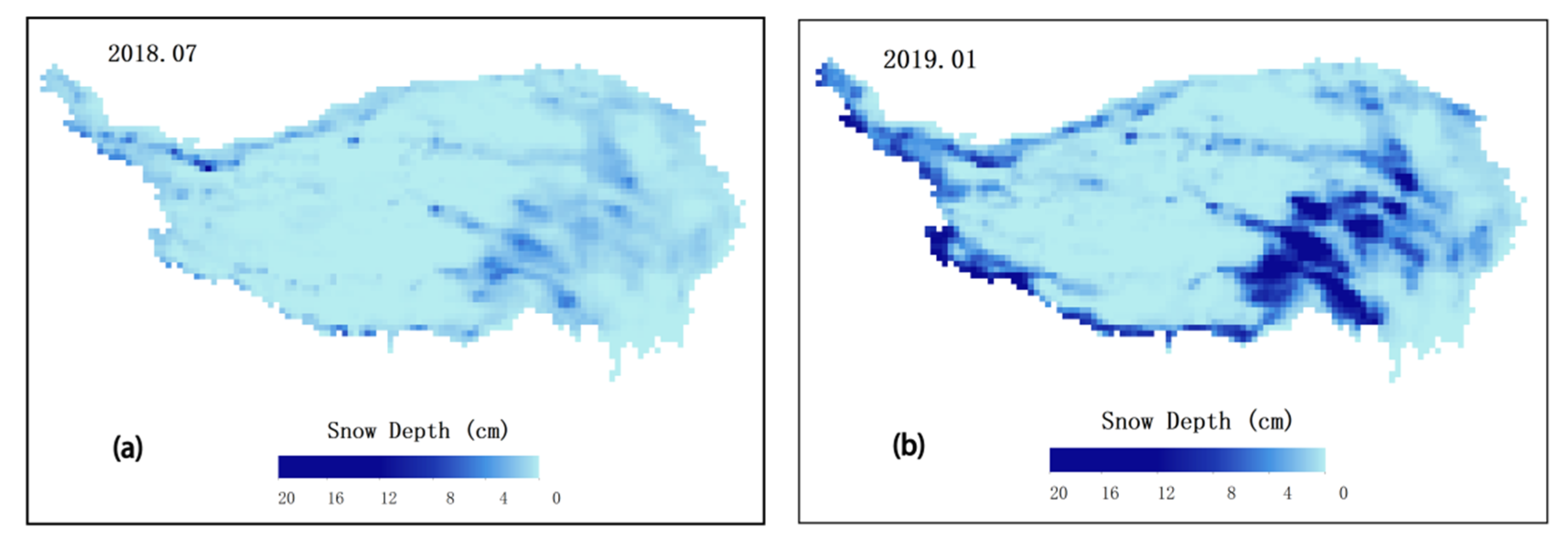
Using this dataset, we calculated the snow cover change in the Tibetan Plateau between January 2018 and December 2019, and the corresponding snow depth changes for four different land cover types. The snow accumulation trend under different land cover types is similar. From October every year, the Tibetan Plateau gradually enters the snowfall period, reaching the peak of snowpack in January and February of the following year. The snow gradually melts after April as the temperature rises. Figure 3 shows the snow depth map of the Tibetan Plateau for one month in summer and winter using this dataset.
By comparing the values with the daily reflectivity data of CYGNSS in the same region, the correlation between snow depth and reflectivity can be inferred, and the potential of CYGNSS in snow feature research can be verified.
2.1.4. SMAP L3 Radiometer Global Daily 36 km EASE-Grid Soil Moisture, Version 7
Previous studies show that GNSS signals reflected from the surface are sensitive to changes in soil moisture, and the soil moisture also changes the SR [22]. This soil moisture product provides a composite of daily estimates of global land surface conditions retrieved by the Soil Moisture Active Passive (SMAP) passive microwave radiometer. The data are on a regular latitude/longitude grid, with predictable disparities in space and time. We used the soil moisture data to plot a time series of mean snow depth with SMAP mean soil moisture with different land cover types on the Tibetan Plateau. For more detail, please see the following. By analyzing the variations in soil moisture over the same period, the effect of SR changes due to soil moisture can be excluded; thus, we believe that the variations of SR are due to the changes of snow coverage.
2.1.5. ERA5 Soil Temperature Data
The dataset is the soil temperature at level 1 (in the middle of layer 1). The European Centre for Medium-Range Weather Forecasts (ECMWF) Integrated Forecasting System (IFS) has a four-layer indication for the soil, where layer 1 ranges from 0 cm to 7 cm. Soil temperature is measured in the middle of each layer. When a freeze–thaw transition occurs in soil, the water in the soil changes from solid ice to liquid water. The dielectric constants of water and ice differ significantly, so the reflectivity changes accordingly. By analyzing the changes in snow depth and SR during the period when the surface temperature does not change from positive to negative (or from negative to positive), we assessed whether the snow depth can be monitored by CYGNSS.
2.2. Calculation of the Surface Reflectivity
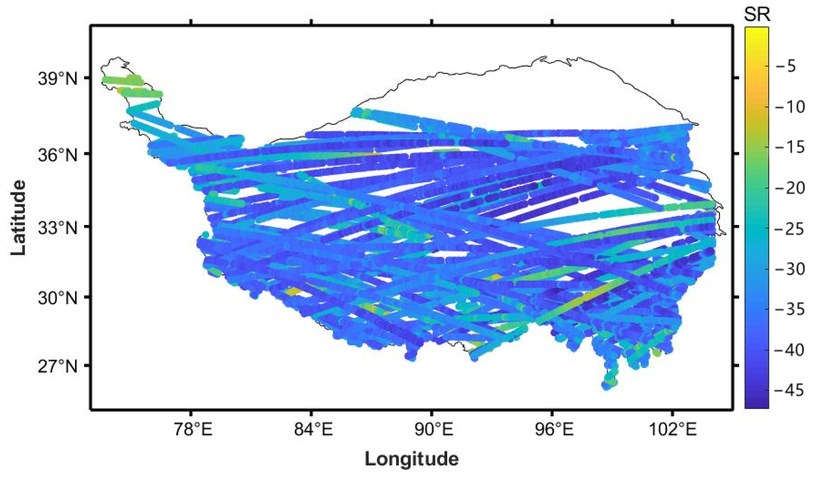
The incidence angle is an important factor affecting the reflectivity of GNSS constellation; the incidence angle of CYGNSS ranges from 0 to 70°. To improve data quality, the incidence angle greater than 60° is eliminated and the data in the direction of the lowest point are used for normalization. Based on the data of CYGNSS L1 from 1 January 2018 to 31 December 2019 in the Tibetan plateau, we calculated and converted all the values to the dB scale, according to Equations (1)–(3). In this paper, we assume that the energy of CYGNSS data is coherent, and incoherent scattering is not considered in the analysis. The effective sampling range of CYGNSS is between approximately 38°N to 38°S, while the latitude range of the Tibetan Plateau is about 26°N to 40°N, so some areas in the north lack data [29]. Figure 4 shows the surface reflectivity of CYGNSS specular points in the Tibetan Plateau on 1 March 2018. Comparing with the satellite image in Figure 1, we can see that the SR is higher in the area with water and snow. In order to exclude the influence of water bodies on the results, these data should be removed from the analysis.
In order to be consistent with the time series analysis, the raw SR of the specular points was transformed into gridded data. Considering the study area and the spatial resolution of snow data (Section 2.1.3), a grid was generated with a resolution of 0.25 along the geodetic latitude and longitude. The data values for each grid cell were defined as the average value of the specular points falling into that grid.
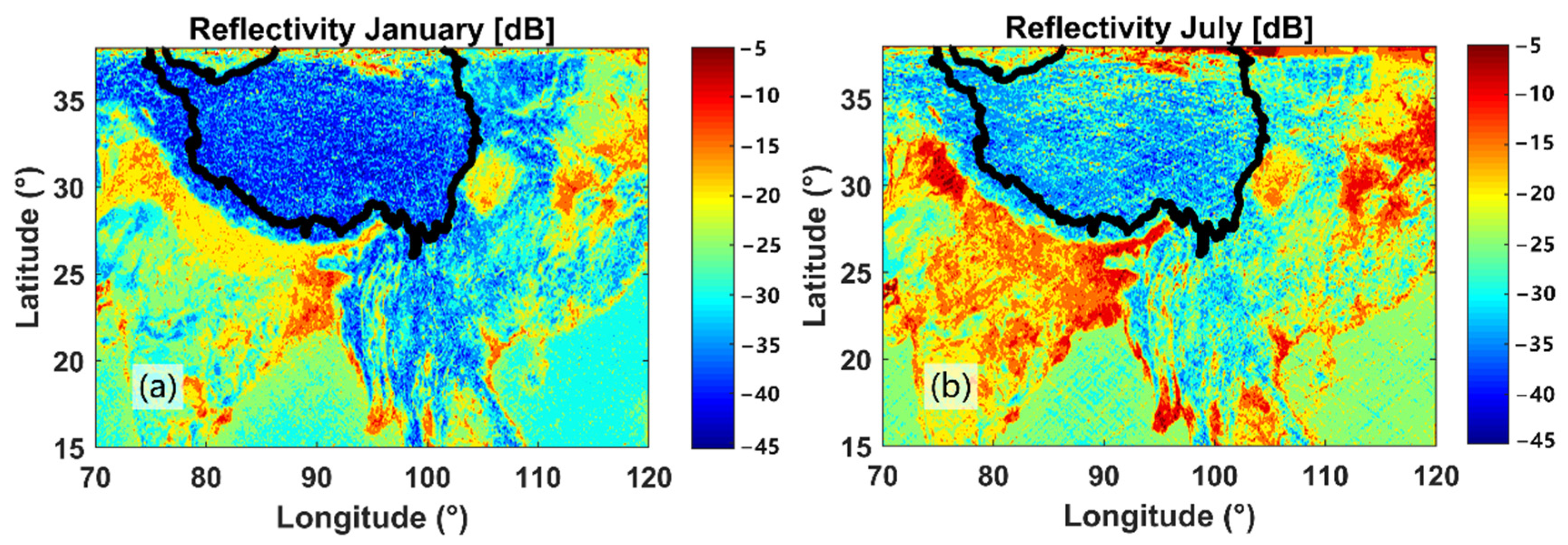
To test the reaction of SR to the changes in surface parameters on the Tibetan Plateau, the SR at the CYGNSS specular reflection points for January 2019 and July 2019 are given in Figure 5a,b. As seen in the figure, the reflectivity increases in the whole region in July compared to January. To exclude differences in CYGNSS observations due to different ground cover types, the variation in SR in response to surface snow depth is analyzed under the same ground cover types.
3. Results and Analysis
3.1. Comparison of Surface Reflectivity and Parameters on the Tibetan Plateau
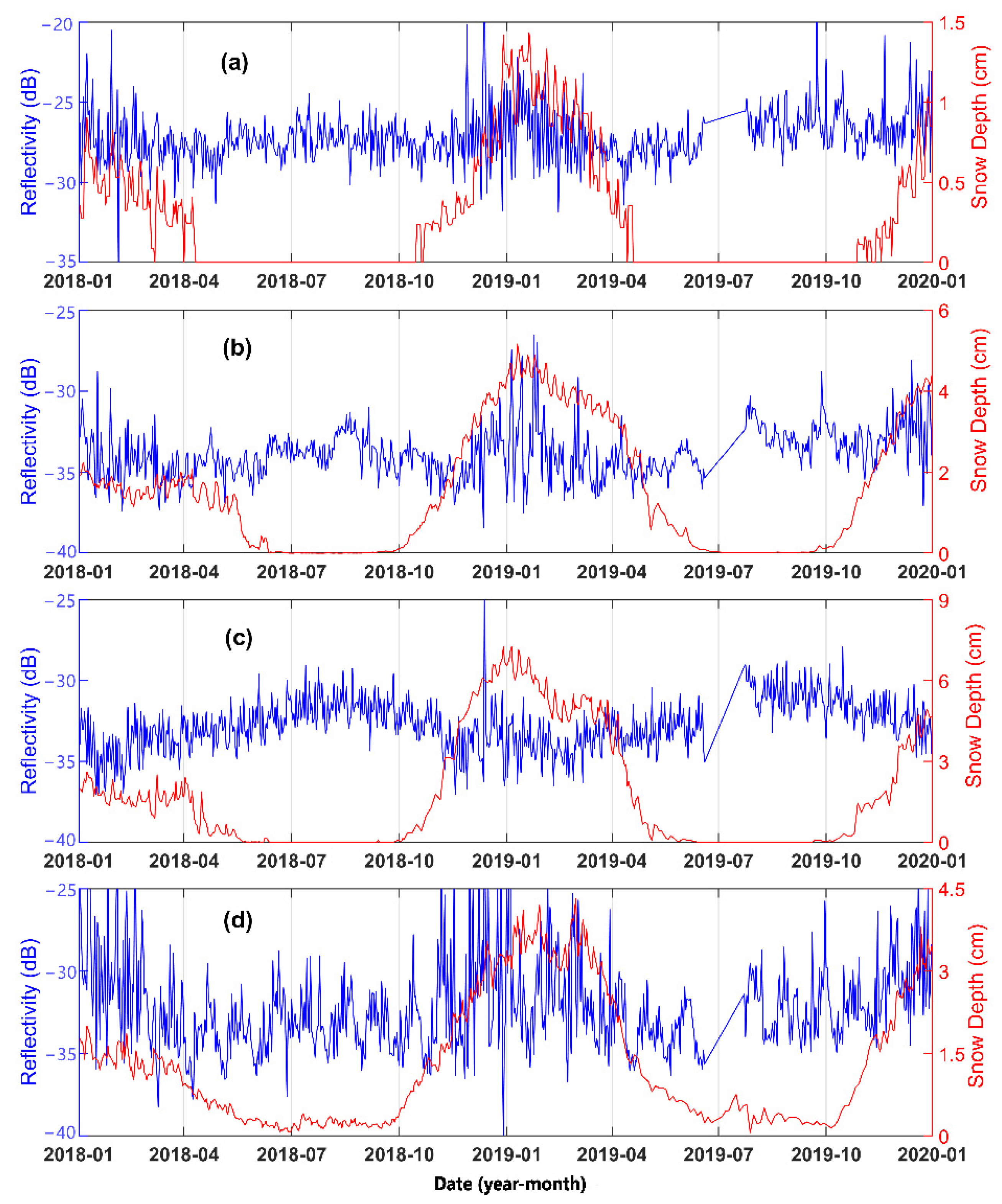
The CYGNSS daily SR and snow depth were analyzed and compared under different land cover types. The snow depth in the Tibetan Plateau region was calculated using the long-term series of daily snow depth dataset in China (1979–2019). Figure 6 shows the time series of CYGNSS SR and snow depth, and we assess the ability of CYGNSS data to monitor changes in snow cover depth by comparing them.
The SR varies with the surface dielectric constant, so there are differences in SR for different ground objects. The snow on the Tibetan Plateau is mainly produced from October to April each year, during which the Tibetan region enters a period of high snow frequency, and SR increases as the snow depth increases. A portion of the SMAP data was lost between June 2019 and July 2019, due to data sampling issues with the satellite. Figure 6 shows the variation of CYGNSS reflectivity (blue left axis), which is consistent with the oscillation of snow depth (red right axis) during the months with snow accumulation. In addition, the part of the anomalous oscillation is mainly caused by the attenuation and volume scattering of vegetation. The change trend of SR and snow depth is closest in the high-vegetation-covered area. In the low-vegetation-covered area and barren/desert area, the CYGNSS time series fluctuates more by the noise, but shows an overall increasing trend. The analysis results show that the CYGNSS SR has a certain correlation with the variation in snow depth, which can be used for snow monitoring on the Tibetan Plateau.
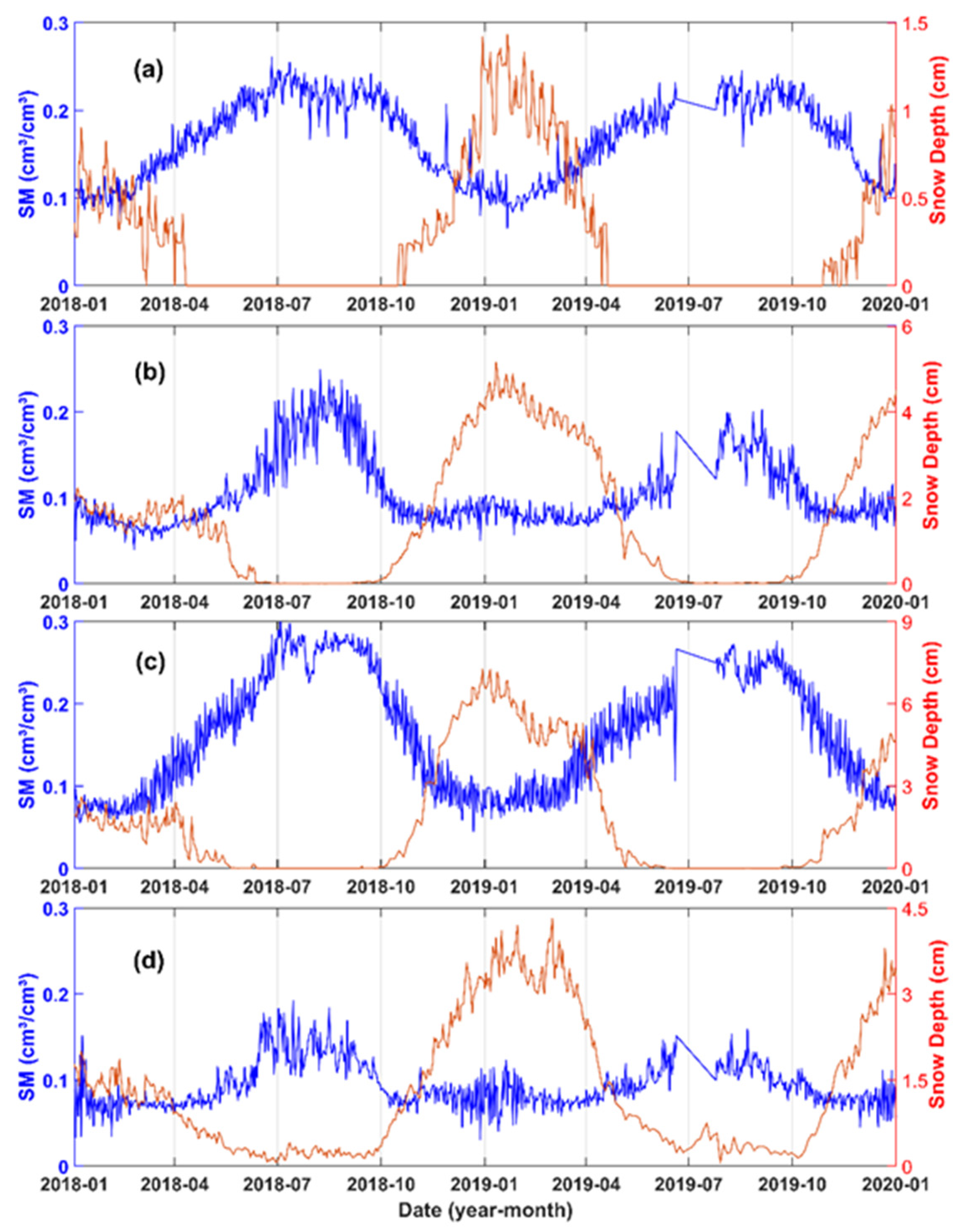
Soil moisture is an important factor affecting SR. To exclude its influence on the results, we plotted the time series of soil moisture using the SMAP surface soil moisture data and examined it with the variation of snow depth over time, in order to investigate the correlation between them. It can be seen from Figure 7 that the interannual variation of soil moisture is closely related to the variation in snow cover, and the soil moisture content fluctuates greatly when the snow cover melts. The low-vegetation-covered area has the largest change in soil moisture. In addition, when the snow cover on Tibetan Plateau is obvious (November 2018–February 2019), the value of soil moisture under different land cover types fluctuates around 0.1 cm³/cm³, and does not change significantly. Therefore, we learn that it is not the change in soil moisture that causes the oscillation of SR.
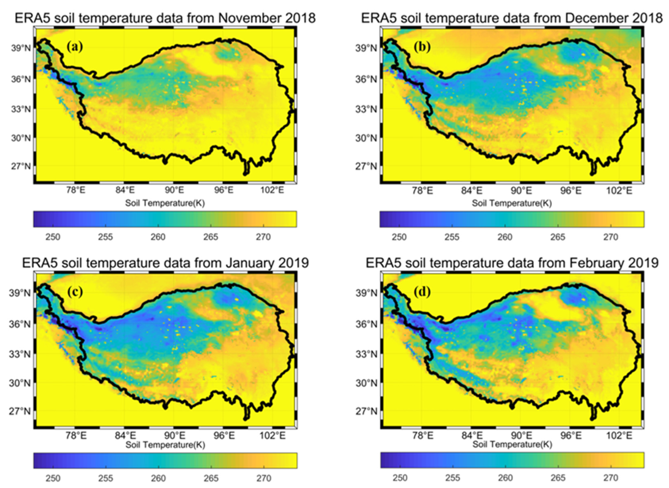
To further verify the effect of snow depth on the SR, we also used the ERA5 soil temperature data to obtain the monthly average soil temperature over this four month period (Figure 8). We found that there is no inversion from negative to positive values of surface temperature in most areas of the Tibetan Plateau during this period. The northern region shows the relatively large temperature variation. However, as this region is beyond the detection zone of CYGNSS, we exclude the effect of surface temperature variations.
Table 2 shows the mean values of snow depth, SR, and soil temperature for the four different land cover types over a four month period. It can be seen that the trends of snow depth and SR over time are approximately the same when the soil temperature is negative without more significant changes. For other commonly used evaluation metrics, such as leading edge slope (LES) and signal to noise ratio (SNR), we provide a brief discussion in Appendix A.
3.2. Surface Reflectivity Difference Ration Factor
In Section 3.1, we evaluated the effects of snow depth on surface reflectivity, and find that it is more sensitive than the other GNSS-R observables, i.e., SNR and LES (Appendix A). Therefore, we provide an indicator in this section to illustrate its effect on the detection of snow properties. Here, we define this indicator as surface reflectivity–difference ratio factor (SR–DR factor) [36]. The factor SR–DR is defined as follows:
where Γ(t) is the SR at time t, and and are the maximum and minimum SR in the time range, respectively. It should be noted that within the form of this equation, the snow water equivalent (SWE) can be achieved when the SWE is in quite good relationship with snow depth.
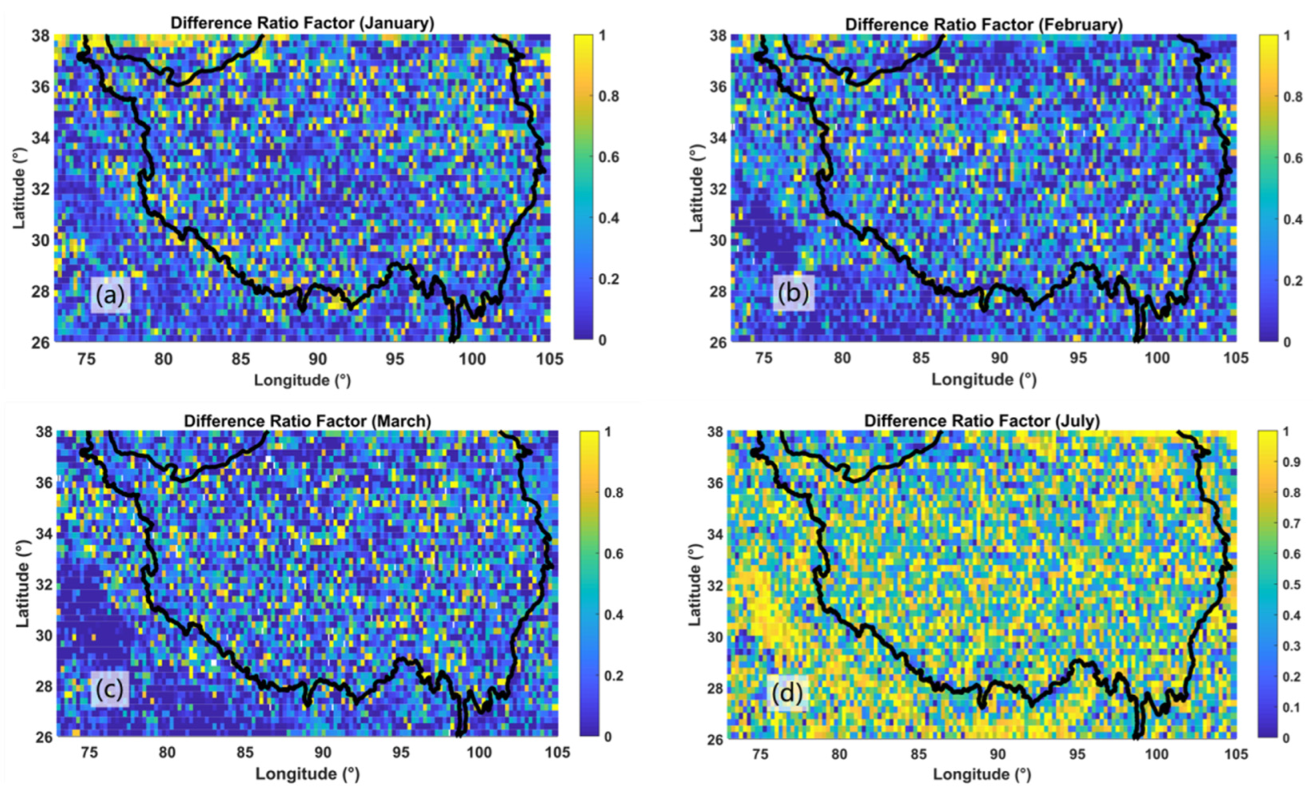
The CYGNSS data for 2019 was studied as a case study. Figure 9 shows the SR–DR factor for the Tibetan Plateau in January, February, March, and July 2019, which has the same resolution of 25 km as SR. Analyzing the factor for the Tibetan Plateau in 2019, we found that the SR–DR factor increases in summer compared to winter for the whole region. It also changes with snow depth in winter when there is snow cover on the Tibetan Plateau.
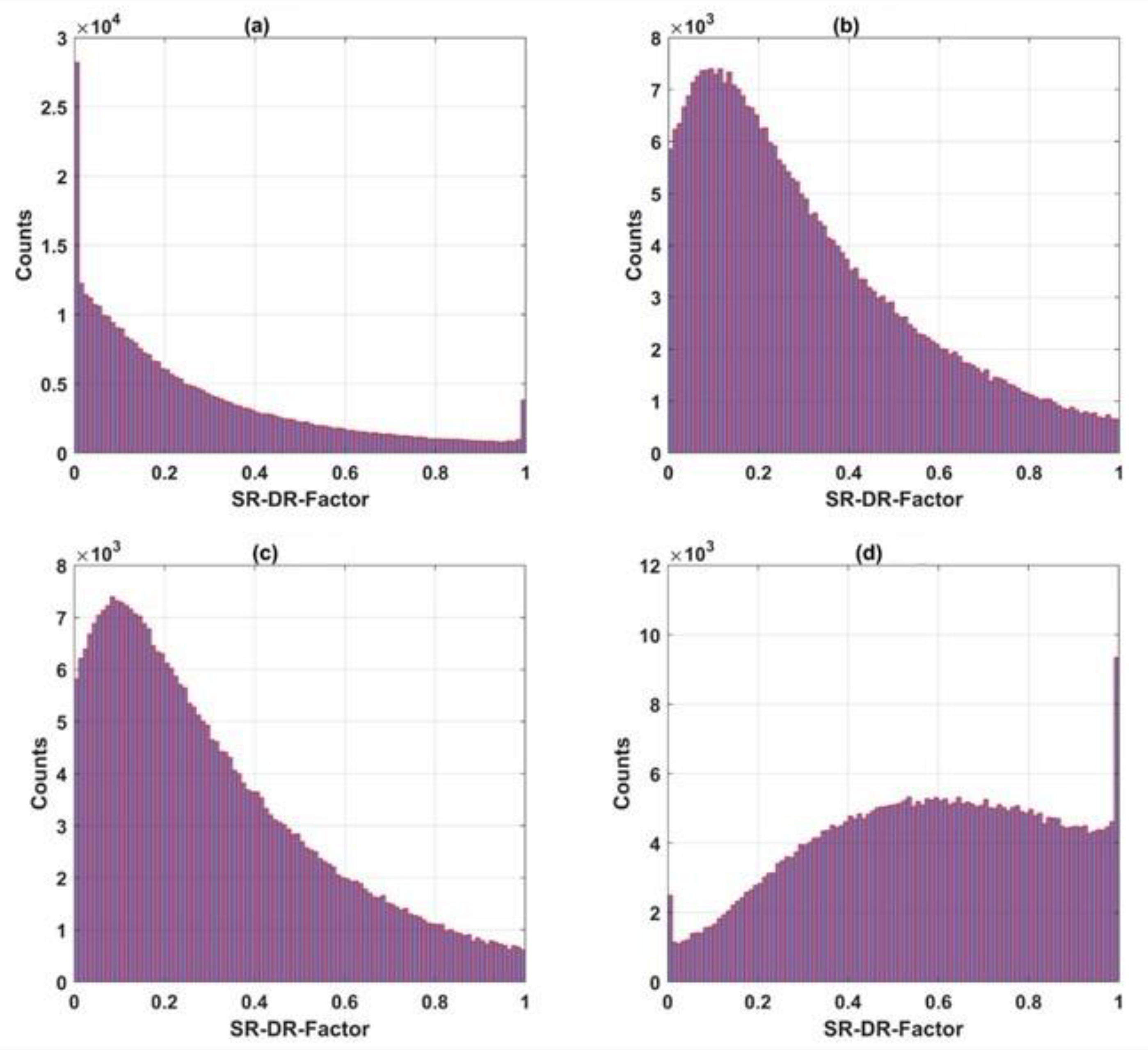
Figure 10 shows that the SR–DR factor for January 2019 is mainly concentrated between 0 and 0.4. In February and March 2019, SR–DR factor shows an increase, without a large change in soil moisture during this period. In July, it shows a higher value, mostly greater than 0.4. The snow depth is also lower at this time, due to the arrival of summer.
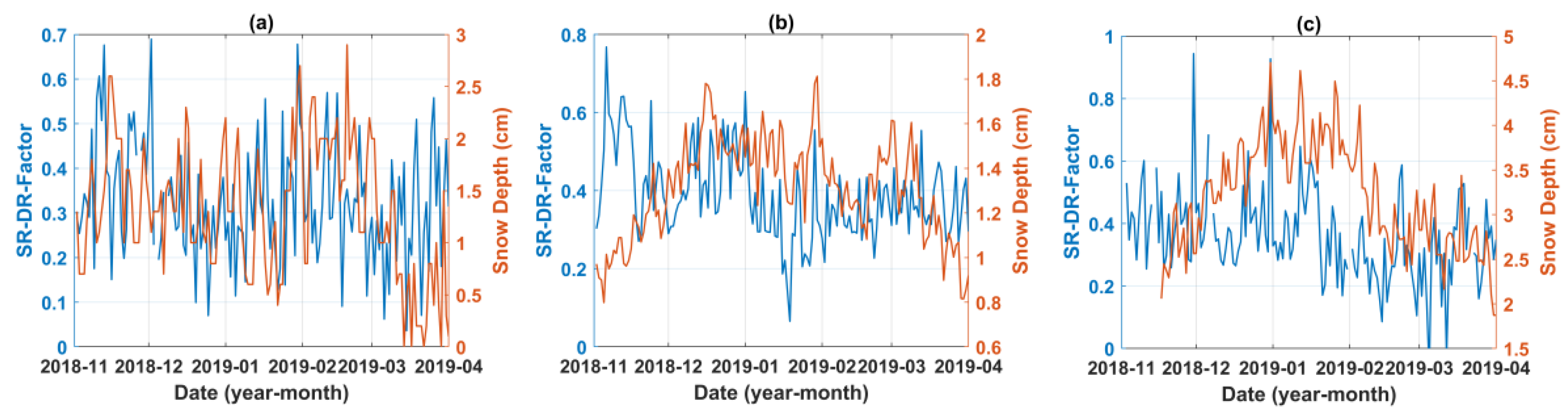
We selected a 1° × 1° size area with different land cover types for the analysis of the relationship between the SR–DR factor and snow depth as follows: (a) barren or desert area (79°–80°E, 33°–34°N); (b) low-vegetation-covered area (81.5°–82.5°E, 31.5°–32.5°N); and (c) moderate-vegetation-covered area (95°–96°E, 29°–30°N). We removed the high-vegetation-covered area because this part of the Tibetan Plateau is small and mostly concentrated in mountainous areas with complex topography. The topographic relief and vegetation roughness may have a great impact on the effective surface reflectivity, which will make the results inaccurate. The time with snow cover on the Tibetan Plateau is concentrated from November to March of the following year, so we choose CYGNSS data from November 2018 to March 2019, and the snow depth at the coordinates of the center point of the area is used to express the change in snow accumulation. Figure 11 presents the time series of SR–DR factor versus snow depth in the research area. From the simulation, we can see that the oscillation of the snow depth in the barren area is, in general, consistent with the daily CYGNSS SR–DR factor. The differences become progressively larger as the vegetation cover level increases.
4. Conclusions
Since the launch of GNSS-R satellites, many scholars have used them to study the parameters of wetland dynamics, sea surface wind speed, and soil freeze/thaw. This paper takes CYGNSS as an example to study its potential application in snow monitoring on the Tibetan Plateau. The CYGNSS data collected from January 2018 to December 2019 were processed and analyzed to calculate surface reflectivity and compare it with snow depth. Soil moisture from SMAP and temperature data from ERA5 were used to study the changes in both when the snow depth varied significantly.
With the help of typical GNSS-R observables (LES, SNR, and SR), we found that SR can be a good potential parameter to indicate the snow depth. Therefore, based on the SR, the finally developed indicator, which is the SR–DR factor, shows an apparent good relationship with snow depth. This factor can represent the snow water equivalent to some extent through the ratio form in the equation.
Compared with conventional remote sensing satellites, the sampled data from CYGNSS have high spatial and temporal resolution. This demonstrates the potential of satellite-based GNSS-R to monitor snow depth at a high spatial resolution.
In the analysis of GNSS-R data, it is generally believed that the signal received by the receiver is mainly composed of coherent scattering along the mirror direction, but, in fact, the incoherent scattering affects the results, and their relative contribution depends on the receiver height, surface roughness, and vegetation coverage. In this paper, only the case of coherent scattering is considered.
The CYGNSS was originally intended for sea surface wind field research, and many of its applications on land are exploratory studies. This paper qualitatively proves that satellite-based GNSS-R can be used for snow monitoring, but still lacks a quantitative evaluation to determine the specific value of snow depth as retrieved from SR. It can be further analyzed with other estimators in future research. In addition, the coverage of CYGNSS is mainly concentrated in the middle and low latitudes, so there is a lack of effective data in some areas of the northern Tibetan Plateau. In practical application, it may be necessary to combine the traditional remote sensing satellite data to achieve high-precision snow monitoring.
Author Contributions
W.M. analyzed and interpreted the data and materials, and wrote the original manuscript. L.H. provided the data analysis and interpretation. X.W. conducted the conceptualization suggestions, review, and funding. S.J. performed the suggestion and inspection. W.B. and X.L. conducted the suggestions and funding. All authors have read and agreed to the published version of the manuscript.
Funding
This research was funded by the National Natural Science Foundation of China (No. 42061057&42074042&72004017), Chifeng University, the Laboratory of National Land Space Planning and Disaster Emergency Management of Inner Mongolia (CFXYZD202006), and Innovative Teams of Studying Environmental Evolution and Disaster Emergency Management of Chifeng University in China under grant number cfxykycxtd202006.
Data Availability Statement
The datasets analyzed during the current study are available from NASA, https://podaac.jpl.nasa.gov/dataset/CYGNSS_L1_CDR_V1.0 (accessed on 12 March 2021). The datasets analyzed during the current study are available in the Land Processes Distributed Active Archive Center, https://lpdaac.usgs.gov/products/mcd12c1v006/ (accessed on 13 January 2022). The datasets analyzed during the current study are available in the National Tibetan Plateau Data Center repository, http://data.tpdc.ac.cn/zh-hans/data/df40346a-0202-4ed2-bb07-b65dfcda9368/ (accessed on 10 August 2020). The datasets analyzed during the current study are available in the National Snow and Ice Data Center (NSIDC), https://nsidc.org/data/SPL3SMP/versions/7 (accessed on 22 December 2021). O’Neill, P.E.; Chan, S.; Njoku, E.G.; Jackson, T.; Bindlish, R.; Chaubell, J. 2020. SMAP L3 radiometer global daily 36 km EASE-grid soil moisture, version 7. [Indicate subset used]. Boulder, CO, USA. NASA National Snow and Ice Data Center Distributed Active Archive Center. https://doi.org/10.5067/HH4SZ2PXSP6A (accessed on 23 December 2021). The datasets analyzed during the current study are available in the ECMWF Reanalysis v5—Land, https://www.ecmwf.int/en/forecasts/dataset/ecmwf-reanalysis-v5-land (accessed on 6 January 2021) [25].
Acknowledgments
The authors acknowledge Zhounan Dong in the Shanghai Astronomical Observatory, Chinese Academy of Sciences, and Andrés Calabia in Nanjing University of Information Science and Technology for their help during the data processing.
Conflicts of Interest
The authors declare no conflict of interest.
Appendix A
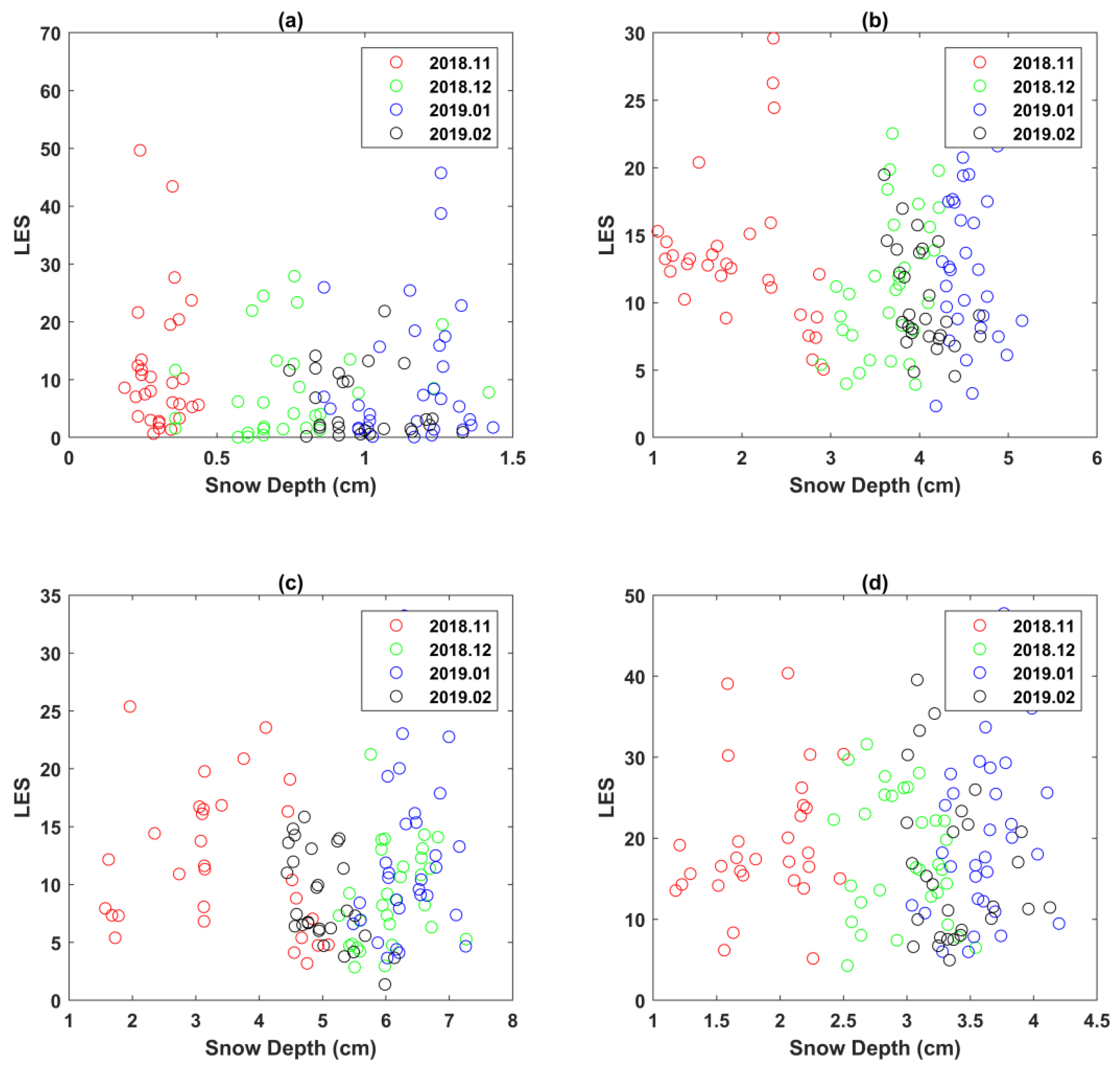
In addition to the qualitative analysis, we also investigated the relationship between the LES of the delayed power waveform commonly used in satellite-based GNSS-R surveys and the snow depth. The LES-SD scatterplot drawn from November 2018 to February 2019 without limiting the satellite observation angle shows there is some relationship between snow properties and LES or SNR. However, the results are not as obvious as SR; therefore, for we employ SR for our analysis.
Appendix A.1. LES and Snow Properties
LES is one of the most important CYGNSS observables. Figure A1 presents the relationship between LES and snow depth. Figure A1a–c are the corresponding relationships for high-, moderate-, and low-vegetation-covered area, while subfigure d is for the barren or desert area. At present, from the relationship shown in Figure A1, we can see that LES has a poor relationship with the snow depth. Since LES is one of parameters that reflects the surface roughness condition, it cannot present the snow depth information in the CYGNSS pixel, which has a spatial resolution of 7 × 2.5 km. However, it isa potential good indicator of snow depth for complex mountain terrain.
Figure A1.
The LES of CYGNSS observations in relation to snow depth in winter. (a) High-vegetation-covered area; (b) moderate-vegetation-covered area; (c) low-vegetation-covered area; (d) barren or desert area.
Figure A1.
The LES of CYGNSS observations in relation to snow depth in winter. (a) High-vegetation-covered area; (b) moderate-vegetation-covered area; (c) low-vegetation-covered area; (d) barren or desert area.

Appendix A.2. SNR with the Snow Properties
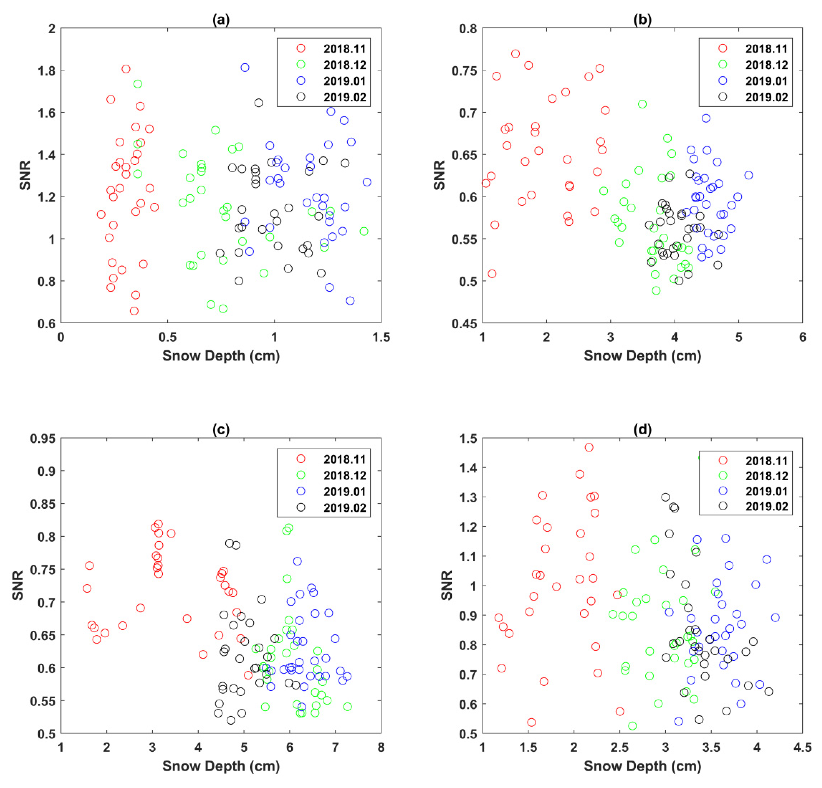
SNR is also one of the most important output parameters of the CYGNSS observables. During our analysis, we also compared the relationship between snow depth and SNR (Figure A2). In order to reduce the influence of different land geophysical parameters, we also plotted the relationship for four different surface types, i.e., high-vegetation-covered area (a); moderate-vegetation-covered area (b); low-vegetation-covered area; (d) barren or desert area (c). We can see that the SNR also cannot reveal the relationship between the two parameters. More detailed analysis to retrieve this information for the detection of snow properties will occur on in our future research.
Figure A2.
The SNR of CYGNSS observations in relation to snow depth in winter. (a) High-vegetation-covered area; (b) moderate-vegetation-covered area; (c) low-vegetation-covered area; (d) barren or desert area.
Figure A2.
The SNR of CYGNSS observations in relation to snow depth in winter. (a) High-vegetation-covered area; (b) moderate-vegetation-covered area; (c) low-vegetation-covered area; (d) barren or desert area.

References
- Brown, R.D. Northern Hemisphere Snow Cover Variability and Change, 1915–1997. J. Clim. 2000, 13, 2339–2355. [Google Scholar] [CrossRef]
- Qiu, J. China: The third pole. Nature 2008, 454, 393–396. [Google Scholar] [CrossRef] [Green Version]
- Cheng, G.D.; Wu, T.H. Responses of permafrost to climate change and their environmental significance, Qinghai-Tibet Plateau. J. Geophys. Res. Atmos. 2007, 112, F02S03. [Google Scholar] [CrossRef] [Green Version]
- Senan, R.; Orsolini, Y.J.; Weisheimer, A. Impact of springtime Himalayan–Tibetan Plateau snowpack on the onset of the Indian summer monsoon in coupled seasonal forecasts. Clim. Dyn. 2016, 47, 2709–2725. [Google Scholar] [CrossRef] [Green Version]
- Bormann, K.J.; Brown, R.D.; Derksen, C. Estimating snow-cover trends from space. Nat. Clim. Change 2018, 8, 924–928. [Google Scholar] [CrossRef]
- Cui, Y.; Chuan, X.; Lemmetyinen, J.; Shi, J.; Jiang, L.; Peng, B. Estimating snow water equivalent with backscattering at X and Ku band based on absorption loss. Remote Sens. 2016, 6, 505. [Google Scholar] [CrossRef] [Green Version]
- Zhou, J.; Kinzelbach, W.; Cheng, G. Monitoring and modeling the influence of snow pack and organic soil on a permafrost active layer, Qinghai–Tibetan Plateau of China. Cold Reg. Sci. Technol. 2013, 90, 38–52. [Google Scholar] [CrossRef]
- Struzik, P. Japan Aerospace Exploration Agency GCOM-W1 satellite snow depth product: Outcome of the first winter. J. Appl. Remote Sens. 2014, 8, 4480–4494. [Google Scholar] [CrossRef] [Green Version]
- Hall, D.K.; Riggs, G.A.; Salomonson, V.V. MODIS snow cover products. Remote Sens. Environ. 2002, 83, 181–194. [Google Scholar] [CrossRef] [Green Version]
- Gafurov, A.; Bárdossy, A. Cloud removal methodology from MODIS snow cover product. Hydrol. Earth Syst. Sci. 2009, 13, 1361–1373. [Google Scholar] [CrossRef] [Green Version]
- Wulder, M.A.; Nelson, T.A.; Derksen, C. Snow cover variability across central Canada (1978–2002) derived from satellite passive microwave data. Clim. Change 2007, 82, 113–130. [Google Scholar] [CrossRef]
- Kim, S.; van Zyl, J.; McDonald, K.; Njoku, E. Monitoring surface soil moisture and freeze-thaw state with the high-resolution radar of the Soil Moisture Active/Passive (SMAP) mission. In Proceedings of the IEEE Radar Conference, Washington, DC, USA, 10–14 May 2010; pp. 735–739. [Google Scholar]
- Derksen, C.; Xu, X.; Dunbar, R.S.; Colliander, A.; Kim, Y.; Kimball, J.S.; Black, T.A.; Euskirchen, E.; Langlois, A.; Loranty, M.M. Retrieving landscape freeze/thaw state from Soil Moisture Active Passive (SMAP) radar and radiometer measurements. Remote Sens. Environ. 2017, 194, 48–62. [Google Scholar] [CrossRef]
- Martin-Neira, M. A passive reflectometry and interferometry system (PARIS): Application to ocean altimetry. ESA J. 1993, 17, 331–355. [Google Scholar]
- Small, E.E.; Larson, K.M.; Braun, J.J. Sensing vegetation growth with reflected GPS signals. Geophys. Res. Lett. 2010, 37, L12401. [Google Scholar] [CrossRef]
- Boyd, D. Inversion Study of Simulated and Physical Soil Moisture Profiles using Multifrequency Soop-Sources. In Proceedings of the IGARSS 2019—2019 IEEE International Geoscience and Remote Sensing Symposium, Yokohama, Japan, 28 July–2 August 2019; pp. 5259–5262. [Google Scholar]
- Masters, D.; Axelrad, P.; Katzberg, S. Initial results of land-reflected GPS bistatic radar measurements in SMEX02. Remote Sens. Environ. 2004, 92, 507–520. [Google Scholar] [CrossRef]
- Comite, D.; Cenci, L.; Colliander, A.; Pierdicca, N. Monitoring Freeze-Thaw State by Means of GNSS Reflectometry: An Analysis of TechDemoSat-1 Data. IEEE J. Sel. Top. Appl. Earth Obs. Remote Sens. 2020, 13, 2996–3005. [Google Scholar] [CrossRef]
- Steve, P. NASA Intensifies Hurricane Studies with CYGNSS. Earth Obs. 2013, 25, 13–21. [Google Scholar]
- Ruf, C.S.; Chew, C.; Lang, T.; Morris, M.G.; Nave, K.; Ridley, A.; Balasubramaniam, R. A New Paradigm in Earth Environmental Monitoring with the CYGNSS Small Satellite Constellation. Sci. Rep. 2018, 8, 8782. [Google Scholar] [CrossRef] [Green Version]
- Chew, C.; Reager, J.T.; Small, E. CYGNSS data map flood inundation during the 2017 Atlantic hurricane season. Sci. Rep. 2018, 8, 9336. [Google Scholar] [CrossRef]
- Kim, H.; Lakshmi, V. Use of Cyclone Global Navigation Satellite System (CyGNSS) Observations for Estimation of Soil Moisture. Geophys. Res. Lett. 2018, 45, 8272–8282. [Google Scholar] [CrossRef] [Green Version]
- Wu, X.R.; Dong, Z.D.; Jin, S.G. First Measurement of Soil Freeze/Thaw Cycles in the Tibetan Plateau Using CYGNSS GNSS-R Data. Remote Sens. 2020, 12, 2361. [Google Scholar] [CrossRef]
- CYGNSS. CYGNSS Level 1 Climate Data Record Version 1.0. Ver. 1.0. PO. DAAC, CA, USA; 2020. Available online: https://podaac.jpl.nasa.gov/dataset/CYGNSS_L1_CDR_V1.0 (accessed on 12 March 2021). [CrossRef]
- Friedl, M.; Sulla-Menashe, D. MCD12C1 MODIS/Terra+Aqua Land Cover Type Yearly L3 Global 0.05Deg CMG V006. 2015, Distributed by NASA EOSDIS Land Processes DAAC. Available online: https://lpdaac.usgs.gov/products/mcd12c1v006/ (accessed on 13 January 2022). [CrossRef]
- Che, T. Long-Term Series of Daily Snow Depth Dataset in China (1979–2020). National Tibetan Plateau Data Center, 2015. Available online: https://data.tpdc.ac.cn/en/data/df40346a-0202-4ed2-bb07-b65dfcda9368/ (accessed on 10 August 2020). [CrossRef]
- O’Neill, E.P.; Chan, S.; Njoku, E.G.; Jackson, T.; Bindlish, R.; Chaubell, J. SMAP L3 Ra-Diometer Global Daily 36 km EASE-Grid Soil Moisture, Version 7. [Soil Moisture]. NASA National Snow and Ice Data Center Distributed Active Archive Center: Boulder, CO, USA, 2020. Available online: https://nsidc.org/data/spl3smp/versions/7 (accessed on 22 December 2021). [CrossRef]
- Muñoz Sabater, J.; ERA5-Land Hourly Data from 1981 to Present. Copernicus Climate Change Service (C3S) Climate Data Store (CDS). 2019. Available online: https://cds.climate.copernicus.eu/cdsapp#!/dataset/10.24381/cds.e2161bac (accessed on 6 January 2021). [CrossRef]
- Ruf, C.; Chang, P.S.; Clarizia, M.P.; Gleason, S.; Jelenak, Z. CYGNSS Handbook; Michigan Pub: Ann Arbor, MI, USA, 2016; p. 154. [Google Scholar]
- Al-Khaldi, M.M. Time-Series Retrieval of Soil Moisture Using CYGNSS. IEEE Trans. Geosci. Remote Sens. 2019, 57, 4322–4331. [Google Scholar] [CrossRef]
- Munoz-Martin, J.F.; Onrubia, R.; Pascual, D.; Park, H.; Camps, A.; Rüdiger, C.; Walker, J.; Monerris, A. Untangling the Incoherent and Coherent Scattering Components in GNSS-R and Novel Applications. Remote Sens. 2020, 12, 1208. [Google Scholar] [CrossRef] [Green Version]
- Garrison, J.L.; Katzberg, S.J.; Howell, C.T. Detection of ocean reflected GPS signals: Theory and experiment. In Proceedings of the IEEE SOUTHEASTCON’97.’Engineering the New Century’, Blacksburg, VA, USA, 12–14 April 1997. [Google Scholar]
- Che, T.; Li, X.; Jin, R.; Armstrong, R.; Zhang, T.J. Snow depth derived from passive microwave remote-sensing data in China. Ann. Glaciol. 2008, 49, 145–154. [Google Scholar] [CrossRef] [Green Version]
- Dai, L.Y.; Che, T.; Ding, Y.J. Inter-calibrating SMMR, SSM/I and SSMI/S data to improve the consistency of snow-depth products in China. Remote Sens. 2015, 7, 7212–7230. [Google Scholar] [CrossRef] [Green Version]
- Dai, L.Y.; Che, T.; Ding, Y.J.; Hao, X.H. Evaluation of snow cover and snow depth on the Qinghai–Tibetan Plateau derived from passive microwave remote sensing. Cryosphere 2017, 11, 1933–1948. [Google Scholar] [CrossRef] [Green Version]
- Carreno-Luengo, H.; Ruf, C.S. Retrieving Freeze/Thaw Surface State From CYGNSS Measurements. IEEE Trans. Geosci. Remote Sens. 2022, 60, 1–13. [Google Scholar] [CrossRef]
Figure 1.
The satellite image of the Tibetan Plateau, Landsat/Copernicus.

Figure 2.
(a) The IGBP land cover type on the Tibetan Plateau; (b) the land cover types on the Tibetan Plateau are reclassified into four types.
Figure 2.
(a) The IGBP land cover type on the Tibetan Plateau; (b) the land cover types on the Tibetan Plateau are reclassified into four types.

Figure 3.
(a) The snow depth map of Tibetan Plateau in summer (July 2018); (b) the snow depth map of Tibetan Plateau in winter (January 2019).
Figure 3.
(a) The snow depth map of Tibetan Plateau in summer (July 2018); (b) the snow depth map of Tibetan Plateau in winter (January 2019).

Figure 4.
CYGNSS specular point surface reflectivity in the Tibetan Plateau on 1 March 2018.

Figure 5.
CYGNSS-derived reflectivity at specular points on Tibetan Plateau in January (a) and July (b) of 2019.
Figure 5.
CYGNSS-derived reflectivity at specular points on Tibetan Plateau in January (a) and July (b) of 2019.

Figure 6.
The time series of SR (blue left axis) versus snow depth (red right axis) compared under different land cover type on Tibetan Plateau. (a) High-vegetation-covered area; (b) moderate-vegetation-covered area; (c) low-vegetation-covered area; (d) barren or desert area.
Figure 6.
The time series of SR (blue left axis) versus snow depth (red right axis) compared under different land cover type on Tibetan Plateau. (a) High-vegetation-covered area; (b) moderate-vegetation-covered area; (c) low-vegetation-covered area; (d) barren or desert area.

Figure 7.
The time series of soil moisture (blue left axis) versus snow depth (red right axis) compared under different land cover type on Tibetan Plateau. (a) High-vegetation-covered area; (b) moderate-vegetation-covered area; (c) low-vegetation-covered area; (d) barren or desert area.
Figure 7.
The time series of soil moisture (blue left axis) versus snow depth (red right axis) compared under different land cover type on Tibetan Plateau. (a) High-vegetation-covered area; (b) moderate-vegetation-covered area; (c) low-vegetation-covered area; (d) barren or desert area.

Figure 8.
The November 2018 to February 2019 monthly average soil temperature on Tibetan Plateau. (a) November 2018, (b) December 2018, (c) January 2019, (d) February 2019.
Figure 8.
The November 2018 to February 2019 monthly average soil temperature on Tibetan Plateau. (a) November 2018, (b) December 2018, (c) January 2019, (d) February 2019.

Figure 9.
The SR–DR factor on Tibetan Plateau in January (a), February (b), March (c), and July (d) of 2019.
Figure 9.
The SR–DR factor on Tibetan Plateau in January (a), February (b), March (c), and July (d) of 2019.

Figure 10.
Histogram of the SR–DR factor distribution on the Tibetan Plateau in January (a), February (b), March (c), and July (d) of 2019.
Figure 10.
Histogram of the SR–DR factor distribution on the Tibetan Plateau in January (a), February (b), March (c), and July (d) of 2019.

Figure 11.
The time series of SR–DR factor versus snow depth. (a) Barren or desert area; (b) low-vegetation-covered area; (c) moderate-vegetation-covered area.
Figure 11.
The time series of SR–DR factor versus snow depth. (a) Barren or desert area; (b) low-vegetation-covered area; (c) moderate-vegetation-covered area.


Table 1.
The Cyclone Global Navigation Satellite System (CYGNSS) level 1 data variables.
| Name | Comment |
|---|---|
| ddm_timestamp_utc | DDM sample time |
| sp_lat | Specular point latitude, in degrees north |
| sp_lon | Specular point longitude, in degrees east |
| sp_inc_angle | The specular point incidence angle, in degrees |
| sp_rx_gain | The receive antenna gain in the direction of the specular point, in dBi |
| gps_eirp | The effective isotropic radiated power (EIRP) of the L1 C/A code signal within ± 1 MHz of the L1 carrier radiated by space vehicle, sv_num, in the direction of the specular point, in Watts |
| rx_to_sp_range | The distance between the CYGNSS spacecraft and the specular point, in meters |
| tx_to_sp_range | The distance between the GPS spacecraft and the specular point, in meters |
| power_analog | 17 × 11 array of DDM bin analog power, Watts |
Table 2.
The mean values of snow depth, SR, and soil temperature for the four different land cover types over a four month period.
Table 2.
The mean values of snow depth, SR, and soil temperature for the four different land cover types over a four month period.
| Time | Snow Depth (cm) | Surface Reflectivity (dB) | Soil Temperature (°C) |
|---|---|---|---|
| (a) Mixed–Forest | |||
| 2018.11 | 0.30817 | –27.36039 | –0.43541 |
| 2018.12 | 0.75975 | –26.51822 | –0.72392 |
| 2019.01 | 1.15806 | –25.96435 | –1.34392 |
| 2019.02 | 0.99447 | –27.32706 | –0.82510 |
| (b) Open–Shrubland (Desert) | |||
| 2018.11 | 1.98258 | –35.25758 | –3.73655 |
| 2018.12 | 3.66645 | –33.51377 | –7.68061 |
| 2019.01 | 4.54840 | –32.83397 | –9.16413 |
| 2019.02 | 4.04246 | –34.33123 | –7.49004 |
| (c) Grassland | |||
| 2018.11 | 3.38779 | –34.03826 | –2.11510 |
| 2018.12 | 6.08088 | –33.24549 | –4.36104 |
| 2019.01 | 6.35053 | –33.78475 | –5.42212 |
| 2019.02 | 5.02427 | –34.37498 | –4.49595 |
| (d) Barren/Desert | |||
| 2018.11 | 1.86681 | –31.47885 | –1.29014 |
| 2018.12 | 2.97565 | –30.19818 | –7.56332 |
| 2019.01 | 3.60599 | –31.14914 | –8.23865 |
| 2019.02 | 3.38220 | –30.62580 | –4.55624 |
Publisher’s Note: MDPI stays neutral with regard to jurisdictional claims in published maps and institutional affiliations. |
© 2022 by the authors. Licensee MDPI, Basel, Switzerland. This article is an open access article distributed under the terms and conditions of the Creative Commons Attribution (CC BY) license (https://creativecommons.org/licenses/by/4.0/).
Share and Cite
MDPI and ACS Style
Ma, W.; Huang, L.; Wu, X.; Jin, S.; Bai, W.; Li, X. Evaluation of CYGNSS Observations for Snow Properties, a Case Study in Tibetan Plateau, China. Remote Sens. 2022, 14, 3772. https://doi.org/10.3390/rs14153772
AMA Style
Ma W, Huang L, Wu X, Jin S, Bai W, Li X. Evaluation of CYGNSS Observations for Snow Properties, a Case Study in Tibetan Plateau, China. Remote Sensing. 2022; 14(15):3772. https://doi.org/10.3390/rs14153772
Chicago/Turabian StyleMa, Wenxiao, Lingyong Huang, Xuerui Wu, Shuanggen Jin, Weihua Bai, and Xuanran Li. 2022. "Evaluation of CYGNSS Observations for Snow Properties, a Case Study in Tibetan Plateau, China" Remote Sensing 14, no. 15: 3772. https://doi.org/10.3390/rs14153772
Note that from the first issue of 2016, this journal uses article numbers instead of page numbers. See further details here.