
Inverse Synthetic Aperture Radar Imaging Using an Attention Generative Adversarial Network


1
Institute of Information and Navigation, Air Force Engineering University, Xi’an 710077, China
2
Collaborative Innovation Center of Information Sensing and Understanding, Xi’an 710077, China
3
Key Laboratory for Information Science of Electromagnetic Waves (Ministry of Education), Fudan University, Shanghai 200433, China
*
Author to whom correspondence should be addressed.
Remote Sens. 2022, 14(15), 3509; https://doi.org/10.3390/rs14153509
Submission received: 15 June 2022
/
Revised: 15 July 2022
/
Accepted: 19 July 2022
/
Published: 22 July 2022
Abstract
:The traditional inverse synthetic aperture radar (ISAR) imaging uses matched filtering and pulse accumulation methods. When improving the resolution and real-time performance, there are some problems, such as the high sampling rate and large amount of data. Although the compressed sensing (CS) method can realize high-resolution imaging with small sampling data, the sparse reconstruction algorithm has high computational complexity and is time-consuming. The imaging result is limited by the model and sparsity hypothesis. We propose a novel CS-ISAR imaging method using an attention generative adversarial network (AGAN). The generator of AGAN is a modified U-net consisting of both spatial and channel-wise attention. The trained generator can learn the imaging operation from down-sampling data to high-resolution ISAR images. Simulations and measured data experiments are given to validate the advantage of the proposed method.
1. Introduction
Inverse synthetic aperture radar (ISAR) can continuously observe the target of interest without being limited by weather, light, and other conditions [1]. Therefore, it has become an important detection means for military reconnaissance and intelligence acquisition. The range and azimuth resolution of ISAR imaging is related to the radar system bandwidth and imaging accumulation angle. Transmitting a large-bandwidth signal can improve the range resolution, but it is limited in practical application. A large signal spectrum width would increase the amount of echo data, resulting in the complexity of radar system design. Increasing the imaging accumulation angle can improve the azimuth resolution, but it requires a long observation time and is vulnerable to external interference. Moreover, the movement of the ISAR target is generally unstable during a long observation time, which increases the imaging complexity [2,3]. There are also some limitations in the acquisition of ISAR data [4]. For example, data may be polluted or lost in the process of radar measurement, and some pulses or frequencies may be interfered with or used for other functions (such as target search and tracking). Due to the mobility of the target, it is sometimes difficult to obtain sufficient observation data, which cannot meet the needs of traditional high-resolution imaging. CS can reconstruct the signal by using less data than Nyquist sampling, which is widely used in the field of radar signal processing [5]. The CS theory mainly includes three core parts: sparse representation, incoherent observation, and optimal reconstruction. The CS-ISAR imaging method is based on the sparsity of the target echo signal. It can reconstruct the radar target image through nonlinear optimization by using a small number of incoherent measurements of radar data. Many scholars have researched signal sparse representation, measurement matrix design, and reconstruction algorithms, achieving many results [4,5,6,7,8,9]. These methods can be classified as model-driven methods.
CS-ISAR imaging can be considered an inverse problem [10]. The method based on deep learning (DL) has shown its advantages in the field of inverse problem solving such as signal reconstruction [11], image denoising [12], and image restoration [13]. Combining model-based sparse reconstruction and data-driven deep learning, scholars have proposed a “data-model-driven” ISAR imaging method. The first application of this method for radar imaging was the recurrent auto-encoder network based on the iterative shrinkage thresholding algorithm (ISTA) that incorporates SAR modelling [14]. It can be used to form focused images in the presence of phase uncertainties. A deep-learning architecture dubbed the 2D-ADMM-Net (2D-ADN) was proposed. It can achieve effective high-resolution 2D ISAR imaging results under the scenarios of low signal-to-noise ratio (SNR) and incomplete data [15]. A deep learning approach was proposed by mapping autofocus approximate message-passing algorithm into a deep network, dubbed AF-AMPNet. It can achieve well-focused imaging results of better performance and higher efficiency [16]. For data-driven methods, a complex-valued convolutional neural network (CV-CNN)-based image reconstruction network was applied to CS radar imaging [17]. Scholars later proposed a full CNN (FCNN) for ISAR imaging, which could yield high-quality results with limited training data [18].
In summary, the traditional RD algorithm is limited by the integrity of the echoes. Imaging results will be defocused when the echo is uncompleted. The CS algorithm can achieve well-focused imaging using few echoes. The tradeoff between computational complexity and the optimal solution is required. The performance of the reconstructed algorithm is influenced by some parameters that need to be adjusted artificially. The “data-model-driven” methods, such as ADMM-net, can learn from the data to get the optimal parameters. However, they are still restricted by sparse prior hypotheses.
In this paper, we propose an AGAN to achieve CS-ISAR imaging. First, we analyze the mapping relationship between the down-sampling echoes and high-resolution imaging on the basis of the approximate observation model and establish the sparse imaging model. Then, the AGAN is designed to solve the sparse regularization problem. The imaging optimization process is realized by using deep learning methods. Online optimization is turned into offline training which greatly reduces time consumption. In order to improve the imaging quality, we design the multistage decomposition architecture to include inception modules and U-Net. The inception can exact the multiscale feature in each convolution layer. The U-Net can exact the multiscale feature across the whole network. the multiscale feature can be divided into two categories: contribution to the imaging, such as position and amplitude of the scattering points, and interference to the imaging, such as noise and clutter. It is difficult to find and locate the information represented by these features accurately. The adjustable weight coefficients are distributed to each feature. The weight coefficients can be estimated by minimizing the loss function through backpropagation.
The main contributions of the paper are as follows: (i) a deep learning method is proposed to solve the sparse regularization problem. The proposed method is trained offline and reduces the time consumption compared to the iterative optimization algorithms; (ii) a novel structure of a generator is designed to improve the quality of CS-ISAR imaging. The single-scale convolution kernels in U-NET are replaced by several convolution kernels with different scales which enhance the ability to extract multiscale features. Each feature is given a learnable weight, and the useful features of imaging are adaptively selected by minimizing the loss function.
2. Strategy of Generative Adversarial Network
CS radar imaging technology uses the sparsity of radar target echoes in high-frequency areas to reduce the data rate of the radar imaging system. Compared with the direct sampling based on Nyquist theory, it is better to acquire and store data. For CS radar imaging, the quality of the reconstruction algorithm directly affects its practicability. The current reconstruction algorithms mainly have the problem of low computational efficiency and sensitivity to the imaging model. Radar imaging not only needs to ensure imaging accuracy but also usually needs to meet certain real-time requirements. In CS imaging algorithms, reconstruction accuracy and calculation efficiency are a pair of contradictions. It is difficult to solve this contradiction when the radar imaging method based on compressed sensing is used in practice.
After translation compensation, the ISAR imaging model can be represented by a turntable model.
The radar transmitted linear frequency modulation (LFM) signal with a bandwidth of B is
where is the rectangular pulse envelope, is the signal pulse width, is the carrier frequency, and is frequency modulation. is the fast time, is the number of transmitted pulses, T is the pulse repetition period (PRI), and is the slow time.
The echo signal received by the radar can be expressed as
where is the number of scattering points of the target, is the target reflection coefficient of i-th scattering point, and is the corresponding delay. Among them, we ignore the influence of target motion within the pulse duration.
The reference LFM signal is
where is the delay of the reference point.
The echo signal after de-chirp can be expressed as
The Fourier transform of is a frequency-domain sparse signal that contains the distance information we need. After sampling , , and , we can obtain the vectors ,, and . We set as the sparsity coefficient of in the frequency domain, which represents the distribution characteristics of target scattering points in the spatial domain.
The CS imaging model can be expressed as
where is the normalized DFT matrix. is a diagonal matrix composed of . The radar echo can be expressed after compression measurement as
where is the measurement matrix, and is the reconstruction matrix. We use to reduce the data volume needed for imaging.
According to the CS theory, the solution of can be expressed as
According to the RD theory, the solution of can be expressed as
We can use a nonlinear reconstruction algorithm to solve Equation (8), such as CS-OMP [19] and sparse Bayesian [20]. The computational complexity of the CS method is higher than that of the traditional RD method [21]. CS obtains higher-resolution images with fewer measurements in the time domain and space domain.
The purpose of the proposed AGAN is to learn the mapping relationship from to , where is the input of the generator and is the label. From Equation (9), we know that can be obtained by multiplied with two fixed value matrices and . We can set two fixed value matrices as the first and second layers of the network. For convenience, we use as the input data. is the output of the generator.
The purpose of the generator is to generate images infinitely close to the real image, and the purpose of the discriminator is to correctly judge the input that comes from the real image or from the generator. The objective function of the GAN can be expressed as
where represents the operation of expectation, represents the discrimination result of the output of the generator, and represents the discrimination result of the label.
The generator and discriminator use alternating iterative training to continuously improve their performance. First, we initialize the parameters of the generator and discriminator. Then, we put and into the discriminator to calculate the loss function . Next, we update the parameters of the discriminator by using an adaptive momentum (ADAM) algorithm. After that, we put the simulated data into the generator to calculate the loss function . Finally, we update the parameters of the generator using the ADAM algorithm. We repeat the above steps to improve the performance of the generator.
3. Structure of Attention Generative Adversarial Network
The proposed ISAR imaging method is based on AGAN. AGAN is a generative model. The core idea of GAN comes from the game theory. The main structure of GAN is composed of a generator and a discriminator.
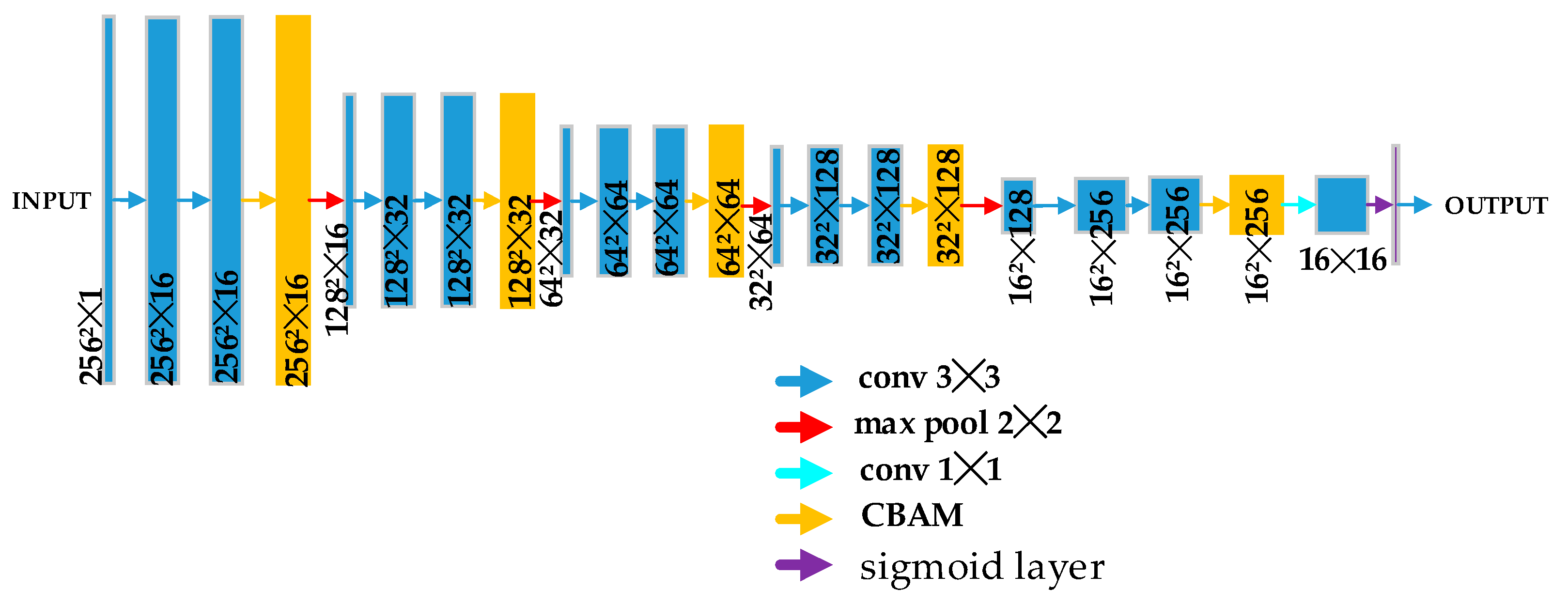
3.1. Generator Architecture
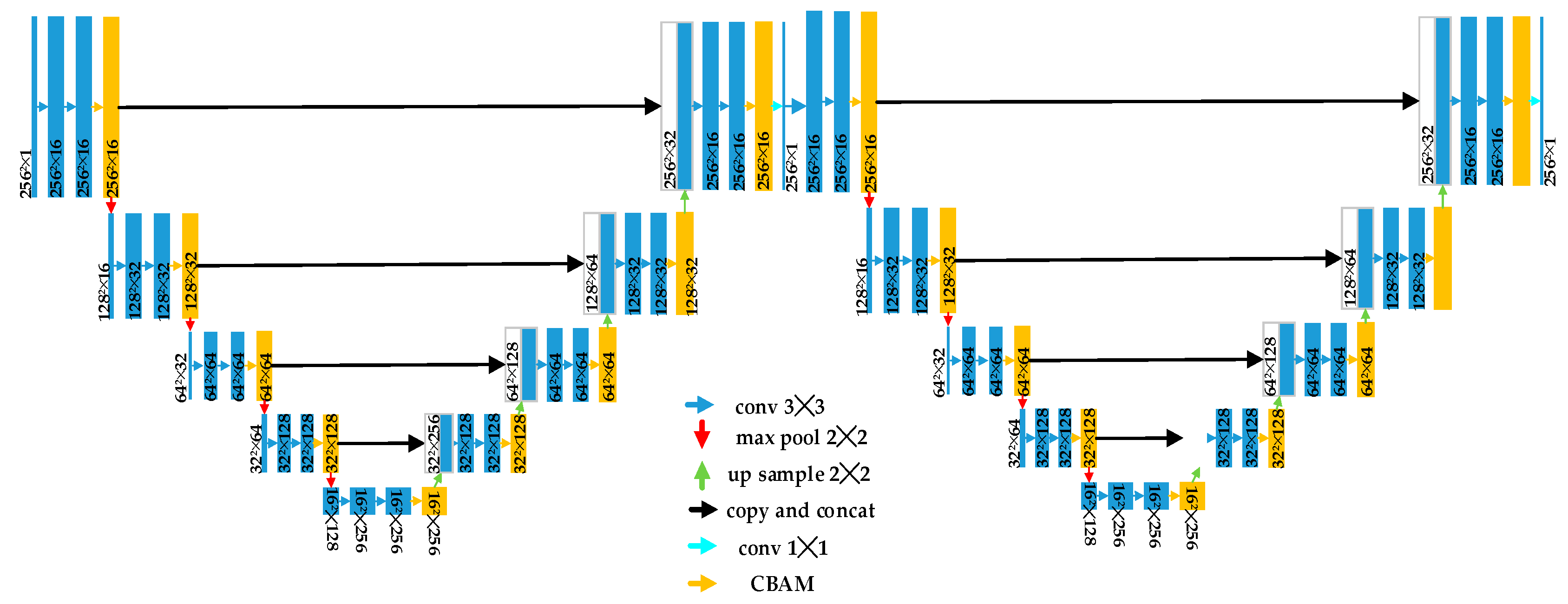
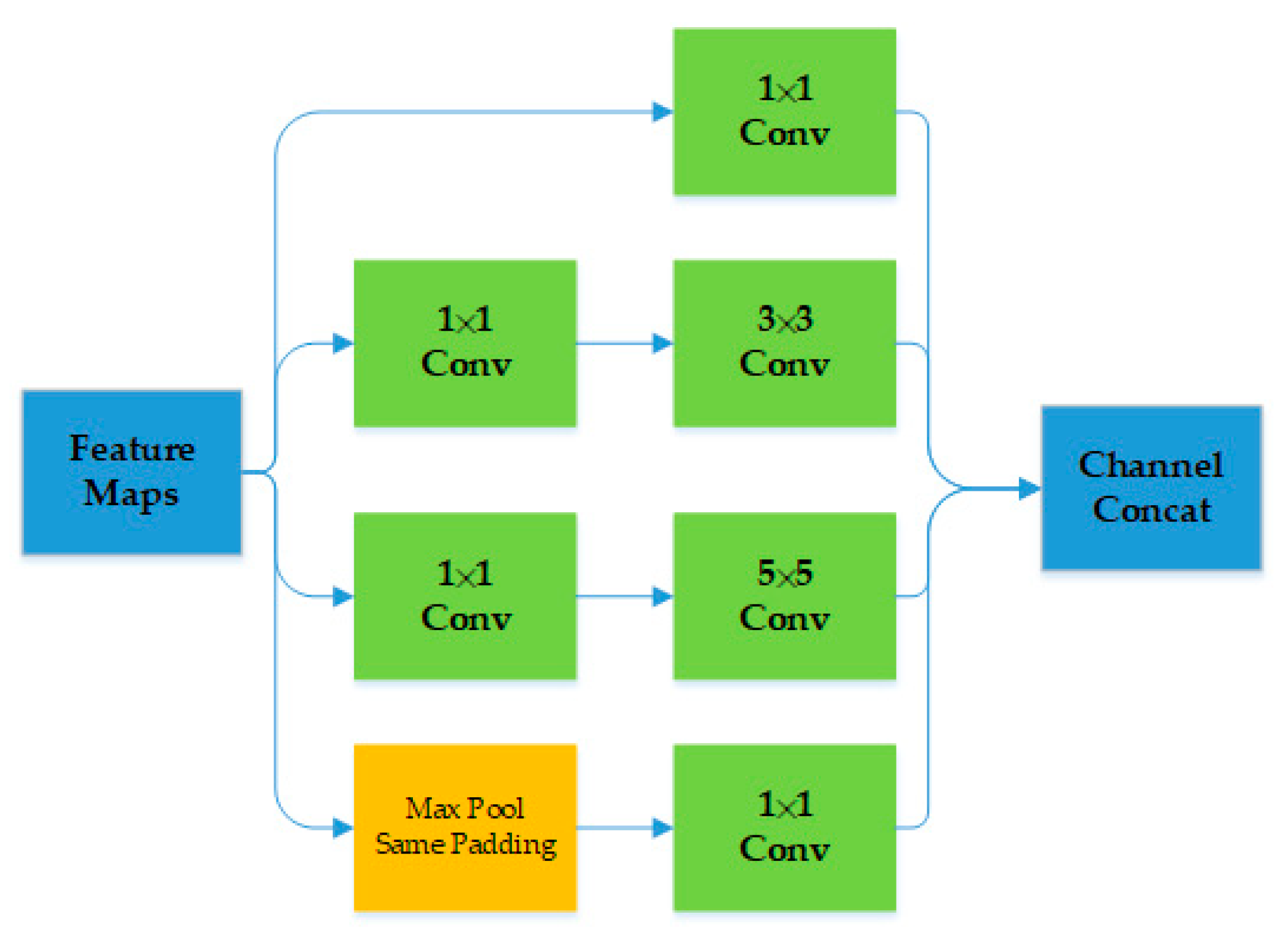
The mapping relationship between the down-sampling echoes and high-resolution imaging is nonlinear and complex. The unique multistage decomposition architecture of U-net has the ability to extract multiscale features compared to the traditional CNN. The skip connection of the U-net combines the local features with the global features through concatenation. The multiscale features fusion is beneficial to the overall image quality, but also retains the details of scattering points. The authors of [18] validated that the U-net has a better performance than the CNN by using a few training samples. As shown in Figure 1, the generator of our method is composed of two modified U-net modules. The structure of both U-net modules is the same. Each module consists of feature extraction blocks, up-sample blocks, skip-connection blocks, and a convolutional block attention module (CBAM). The feature extraction block is used to extract the feature maps from the input. It is composed of two convolution layers and a down-sampling layer. The inception module is used in the convolution layer. As shown in Figure 2, there are convolution kernels of 1 × 1, 3 × 3, and 5 × 5, as well as a max pooling of 3 × 3 with the same padding. The parallel structure increases the width of the network, i.e., the number of neurons in each layer. Using convolution kernels with different sizes means that we can obtain features of different scales, and then better image representation can be obtained by fusing information from different scales. The up-sample block is used to recover the resolution. The bilinear interpolation method is used to achieve up-sampling. The skip-connection block is used to contact the feature. U-net combines shallow and deep features in the channel dimension to form more features. Each feature extraction block and up-sample block has a CBAM module. The CBAM module is composed of a channel attention module (CAM) and a spatial attention module (SAM). The inception and the skip-connection combine the feature maps in the channel dimension. CAM is used to choose feature maps that have a great contribution to imaging. SAM is used to pay more attention to strong scattering points. Using the CBAM module, we can possibly improve the quality of imaging.
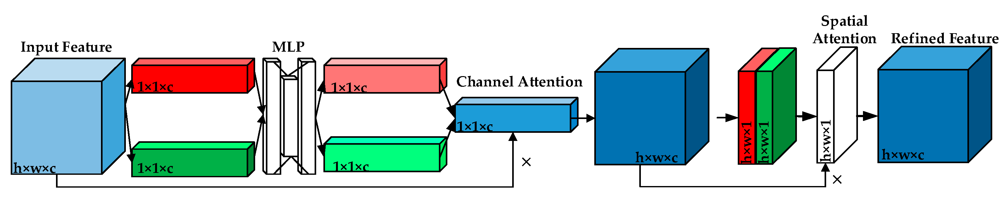
3.2. Convolutional Block Attention Module
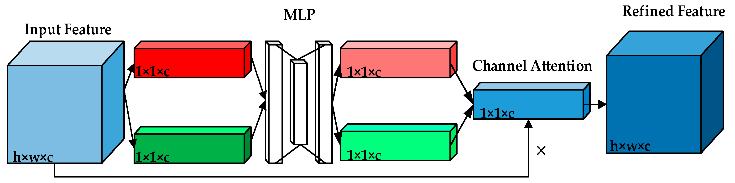
Channel-wise attention: As shown in Figure 3, two feature maps are obtained from the original feature maps Θ through maximum pooling and average pooling, where is the width, h is the height, and c is the number of channels. Then, two feature maps pass through the multilayer perceptron (MLP) module. In this module, they first compress the number of channels and then expand to the original number of channels. Two activated results are obtained through the ReLu activation function [22]. Adding the output results element by element, we can obtain the output result of channel attention through the sigmoid activation function. Finally, we multiply the channel attention to the original feature maps and change it back to the size of . Thus, the channel-wise attention can be expressed as Θ
where represents the original feature, represents the average pooling of , represents the max pooling of , represents the multiplication of the corresponding elements in the two matrices, and is the sigmoid activation function. represent the first- and second-layer weight coefficients of MLP, respectively.
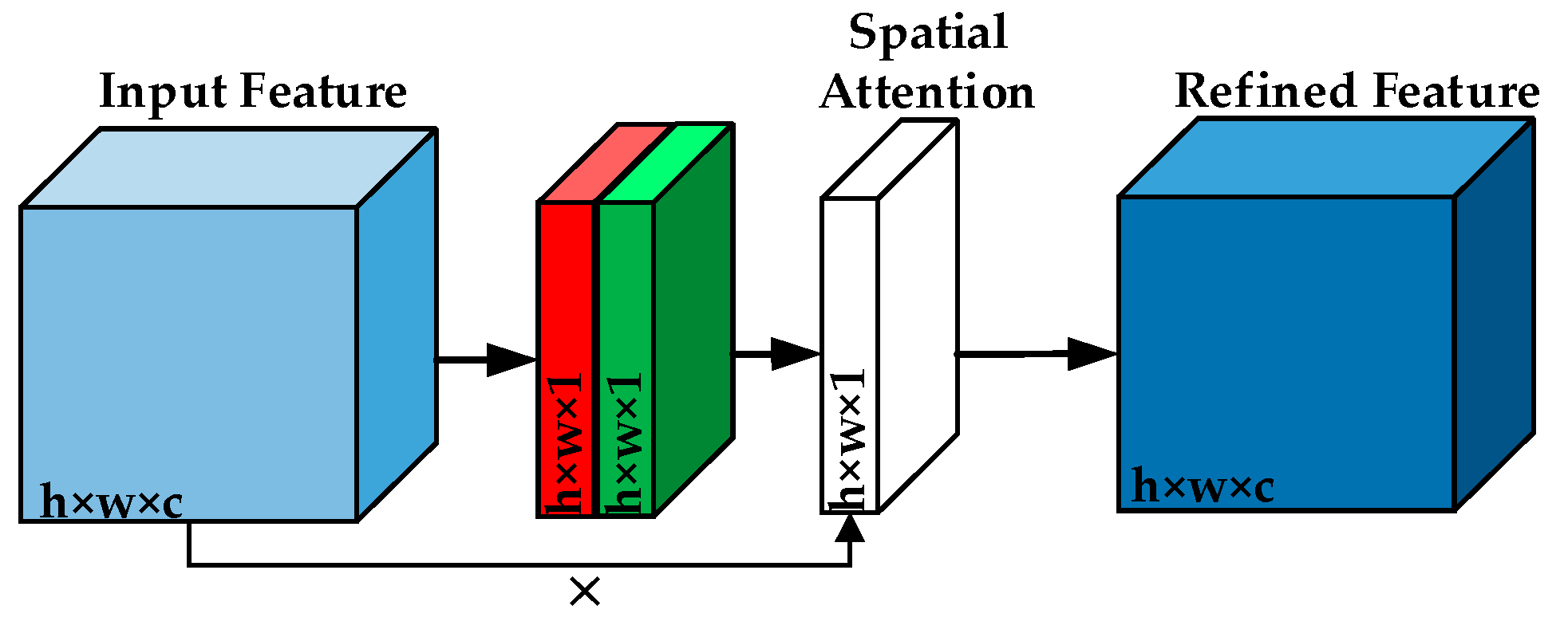
Spatial attention: As shown in Figure 4, two feature maps are obtained from the original feature maps through maximum pooling and average pooling, where w is the width, h is the height, and c is the number of channels. Then, the two feature maps are combined through concatenation operation. 3 × 3 convolution is used to transform the feature map into a feature map. Then the feature map of spatial attention is obtained through a sigmoid. Finally, the output results are multiplied by the spatial attention to original feature maps. Thus, the spatial attention can be expressed as follows:
where represents the original feature, represents the average pooling of , represents the max pooling of , represents the multiplication of the corresponding elements in the two matrices, and is the sigmoid activation function.
Spatial-channel attention: As shown in Figure 5, two submodules of channel attention and spatial attention can be combined in parallel or serial connection. There are also different choices in the sequence of CAM and SAM. In follow-up experiments, the result of the series method with channel attention first was shown to be the best.
3.3. Discriminator Architecture
As shown in Figure 6, the discriminator D is a convolutional network which consists of seven layers. The first five layers use the same structure as the feature extraction block of generator G. The sixth layer is a 1 × 1 convolution layer. The last layer is a sigmoid layer.
4. Experimental Results
In this section, experimental results based on simulated and measured data are presented to demonstrate the effectiveness of the proposed algorithm. The proposed imaging method is compared with the ADMM-net, U-net, CS-OMP, and RD methods.
4.1. Simulated Data
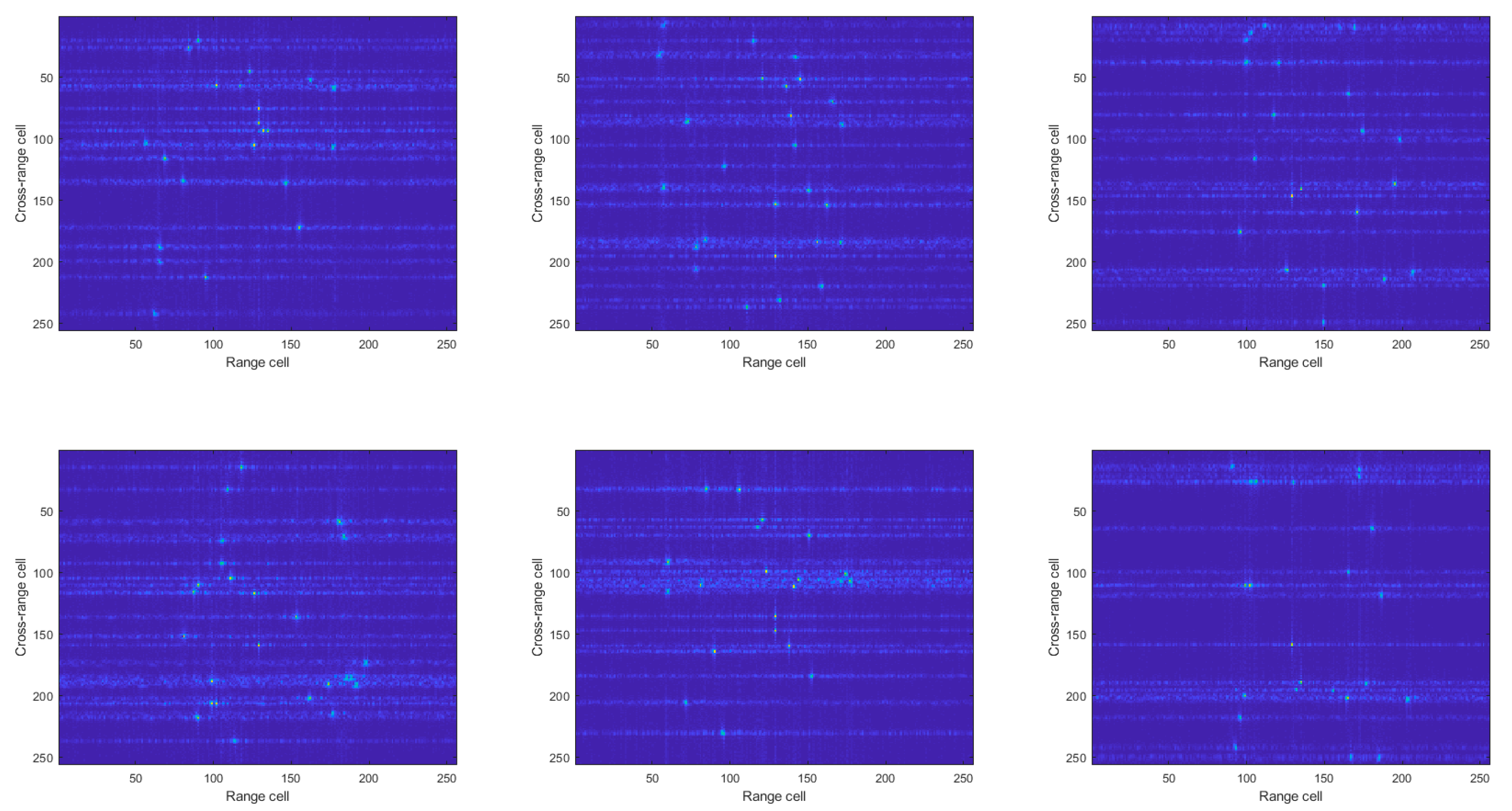
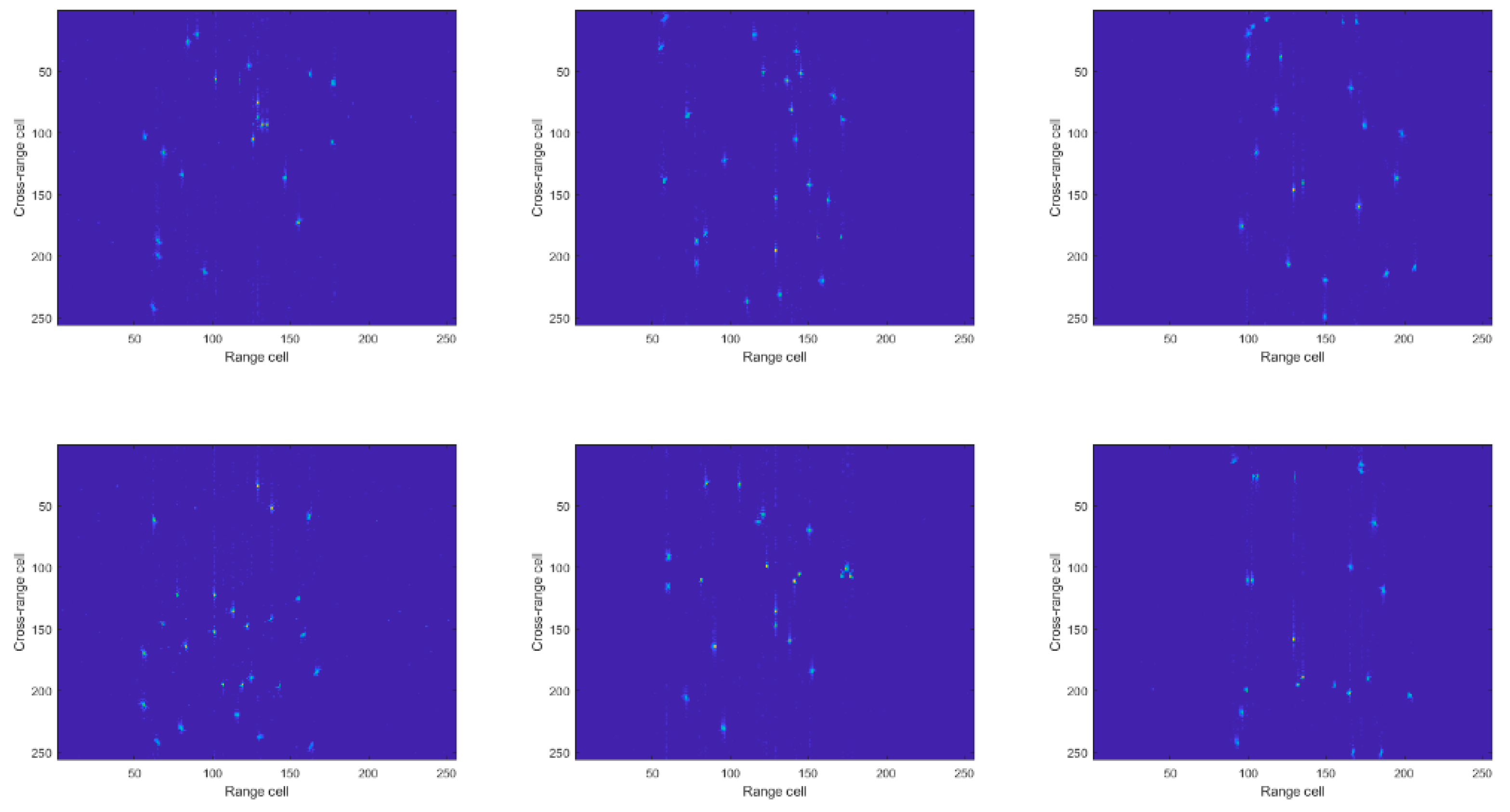
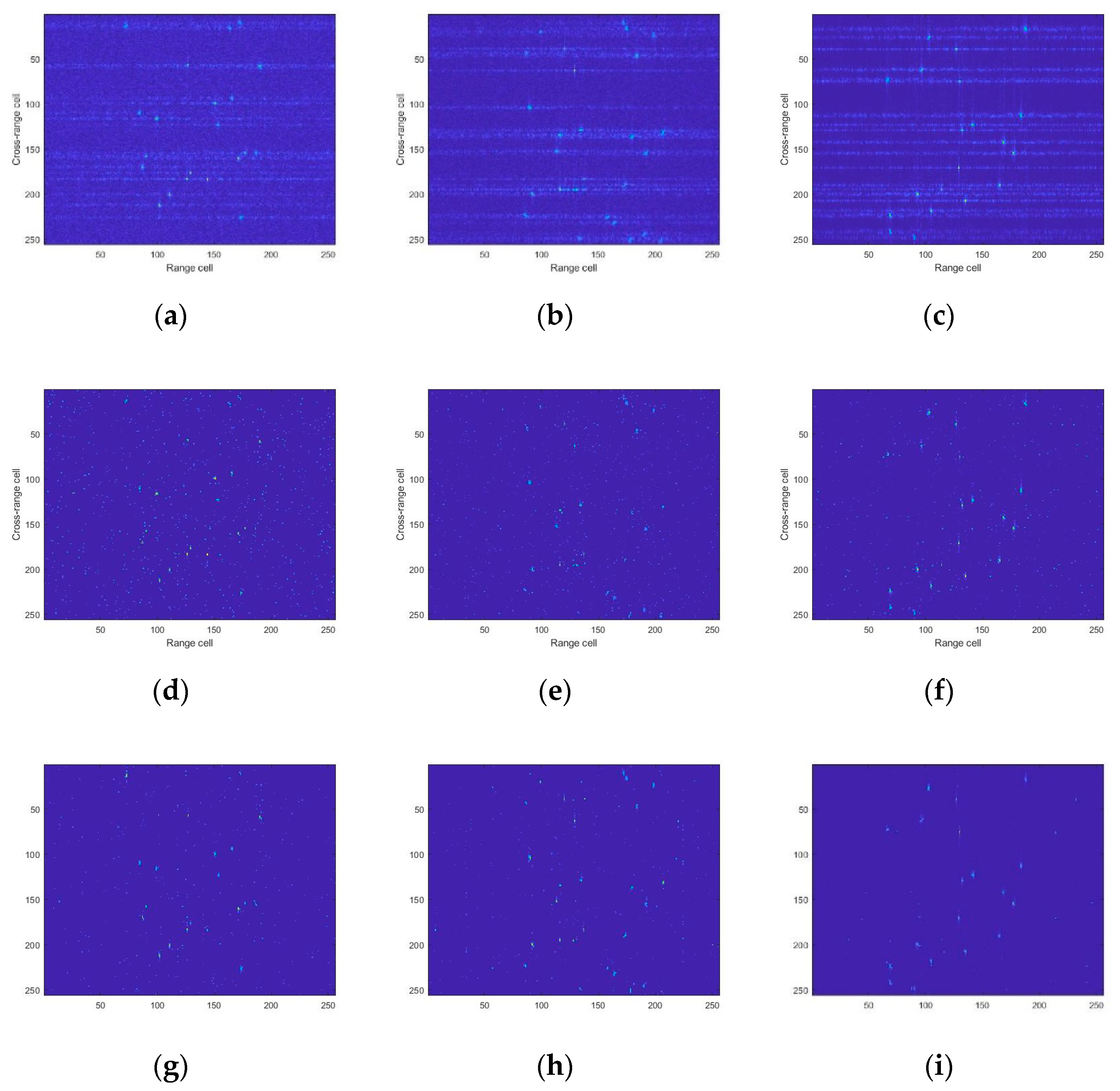
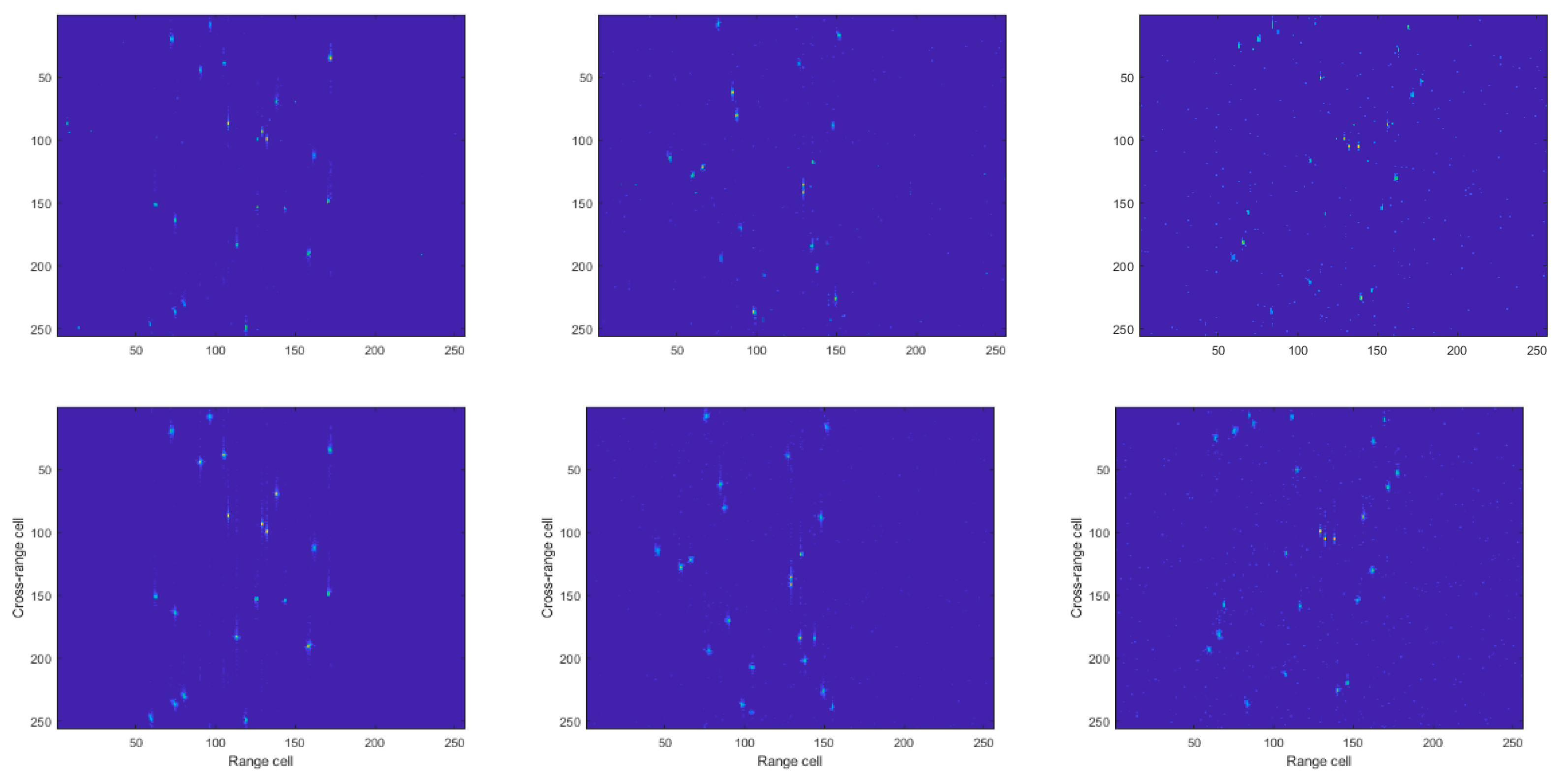
We created an imaging scene in which there were some randomly distributed scattering points. The LFM signal was used to generate echoes. Each echo had 256 slow-time sequences, and each sequence had 256 samples. A total of 5000 different echoes were generated with different scenes. Sparse data were generated using the 30% down-sampling echo based on the RD algorithm, as shown in Figure 7. Labels were generated using full aperture data based on the CS-OMP algorithm, as shown in Figure 8. The simulated radar parameters are shown in Table 1.
4.2. Experiment Results
In order to indicate the performance of algorithms numerically, image entropy (ENT), peak signal-to-noise ratio (PSNR), root-mean-square error (RMSE), and imaging time were used to evaluate the imaging quality.
As shown in Figure 9, the performances of RD, CS, U-net, ADMM-net, and the proposed method were compared. The images generated by the RD algorithm were defocused due to the down-sampled data. The images reconstructed by CS-OMP missed some scattering points. ADMM-net, U-net, and the proposed method achieved well-focused results. The focused performance of ADMM-net method was better than that of U-net. The reconstructed performance of U-net was better than that of ADMM-net. The proposed method produced well-focused images with a clear background and less MSE. The imaging time consumption of the proposed method was 20–30 ms. Compared to CS-OMP, it could significantly reduce time consumption. Table 2 gives the measurements of ENT, MSE, PSNR, and imaging time.
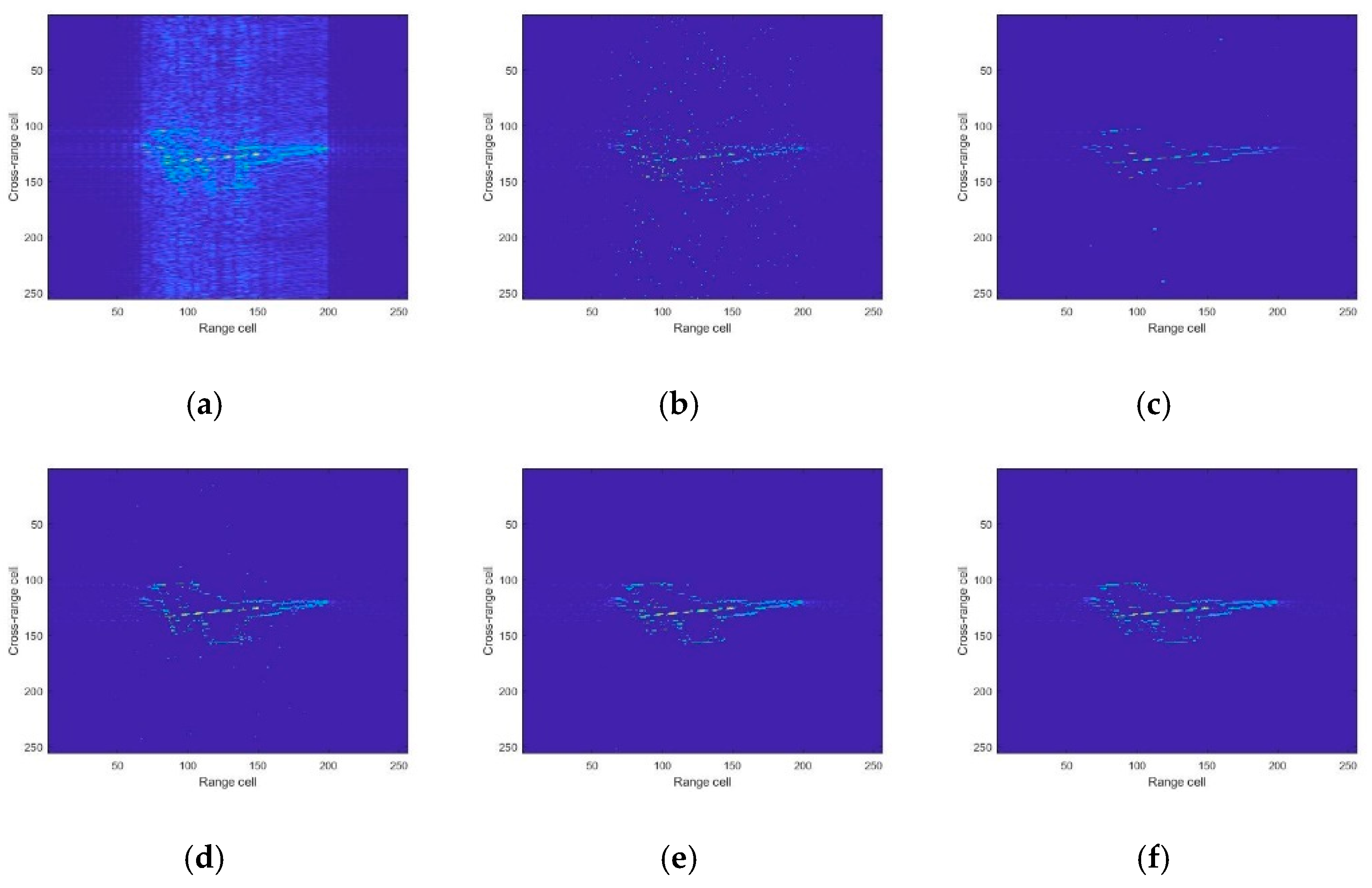
Experiments were also carried out on the measured data of Yak-42 and Mig-25 aircraft. The echoes were expanded to 256 slow-time pulses and 256 samples by interpolation. The image results of Yak-42 and Mig-25 were similar. As shown in Figure 10 and Figure 11, the image of the RD algorithm was defocused. The traditional CS-OMP algorithm could not get well-focused results. ADMM-net, U-net, and the proposed method could all achieve good imaging performance. ADMM-net could learn the key parameters of the CS reconstruction algorithm. The proposed method could get a less noisy background. Compared of two other deep learning methods, the proposed method could get the minimum MSE and maximum PSNR.
In order to further verify the better performance of the proposed method, ablation experiments were conducted.
As shown in Table 3, the best combination was achieved with the channel attention module in the front and the spatial attention module in the back, as indicated in Section 3.2.
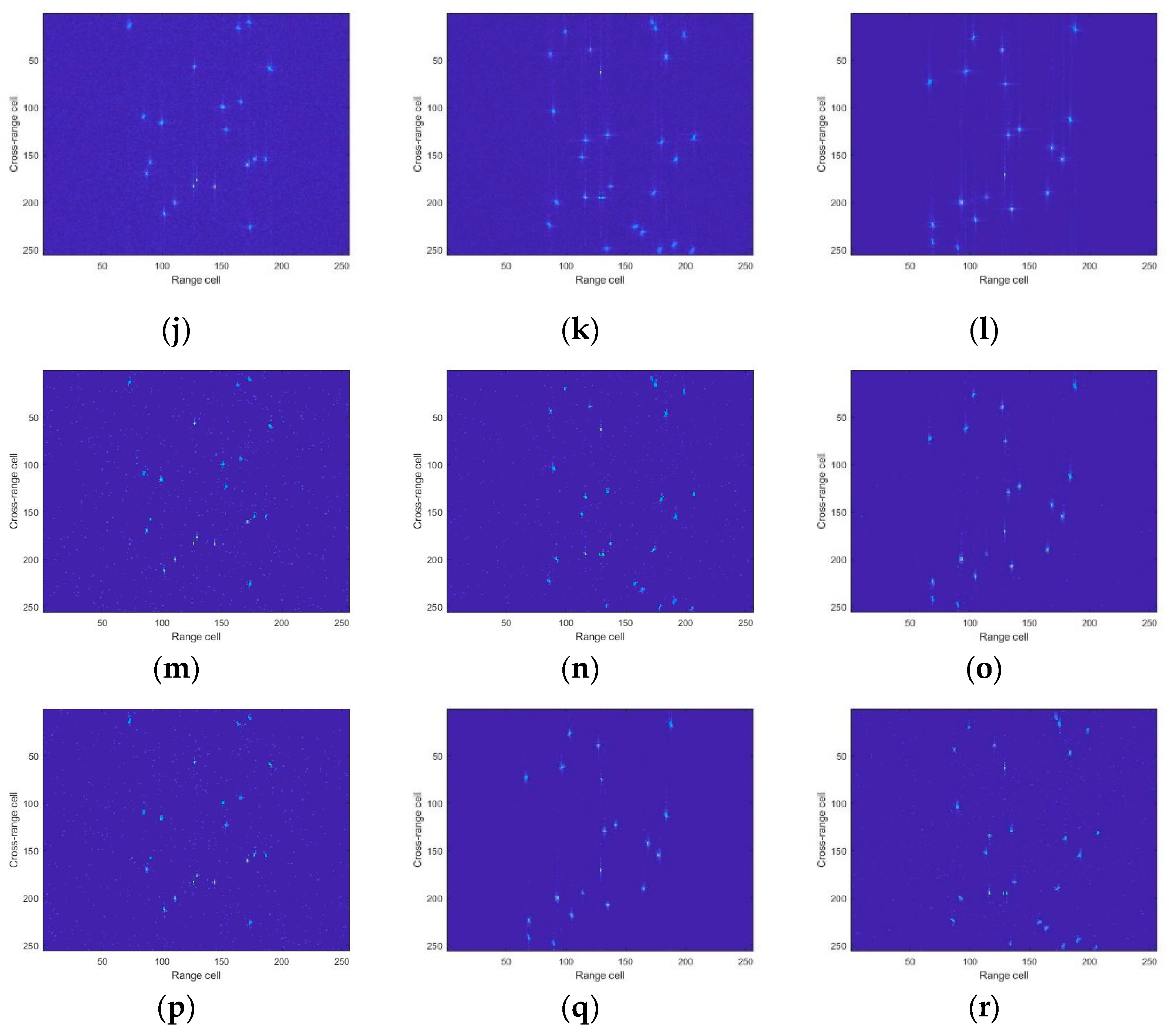
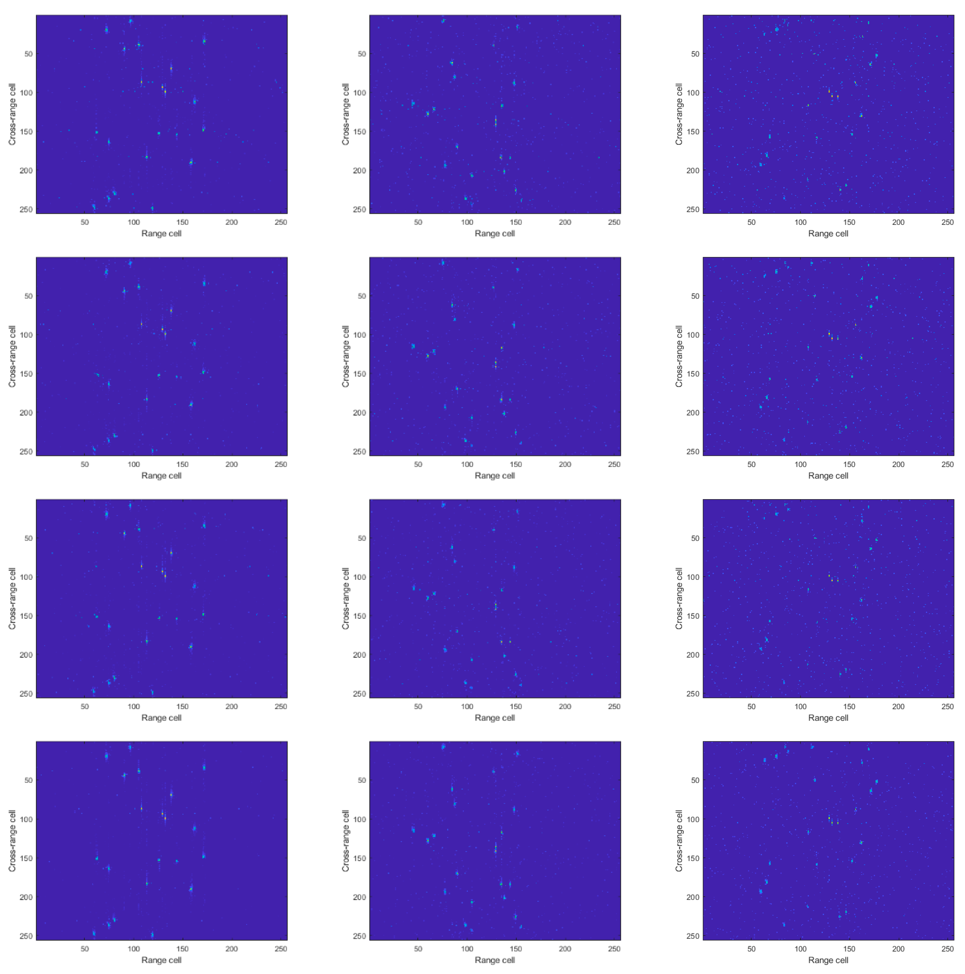
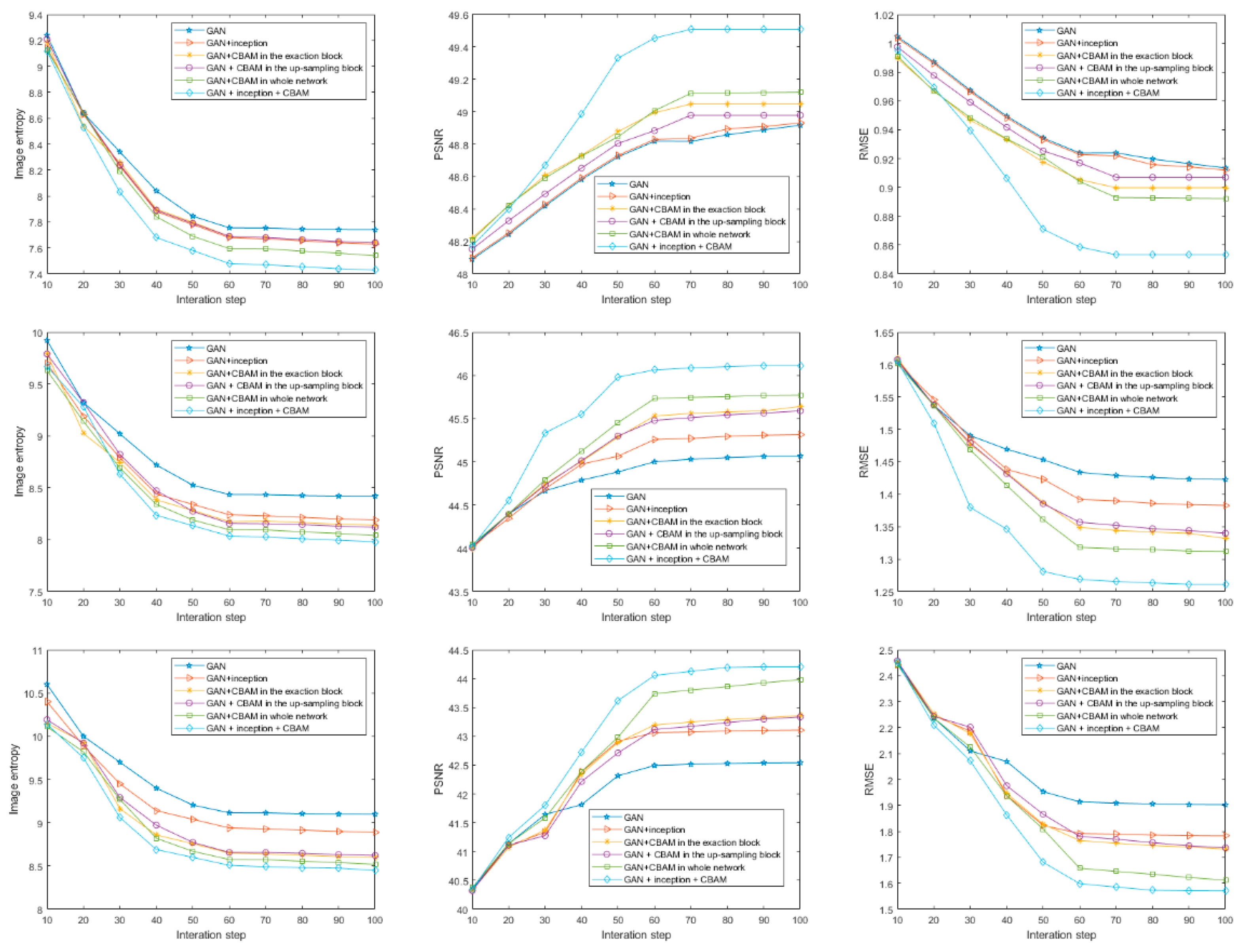
As shown in Figure 12, the performances of GAN, GAN with inception, GAN with CBAM in the exaction block, GAN with CBAM in the up-sampling block, GAN with CBAM in whole network, and the proposed method were compared. From the first to the sixth row, the imaging results of the above methods are shown, respectively. From the first to the third columns, the imaging results with SNR = 10 dB, 5 dB, and 0 dB, respectively, are shown. In Figure 13, from the first to the third rows, the training results with SNR = 10 dB, 5 dB, and 0 dB, respectively, are shown. The simulated data and measured data were used to test the different networks. The test results are shown in Table 4. The proposed method achieved the best imaging result with focused scattering points and a clear background.
The inception structure exacts different features by using convolution kernels of different sizes. The large convolution kernel can extract more global features, which may contribute to scene reconstruction accuracy, while a small convolution kernel can extract more local features, which may contribute to scattering point reconstruction accuracy. The image results of GAN with inception were better than those of GAN and U-net. A low RMSE means that the results have low reconstructed error. A low ENT means that the results have a less noisy background and good focused performance of scattering points. The CBAM module was used to pay different attention to different features. U-Net has a skip-connection structure, which can confuse the features of each layer. Inception can also get different features and compose them using concatenation. When echo SNR is high, the background is clearer. To get a good, reconstructed image, more attention needs to be paid to some special local features. The imaging scene used needs to be sparse. Special attention should be paid to the scattering points. Simulated data can be used to train the network to learn the parameters of CBAM. As shown in Table 4, we can see that using CBAM can improve the quality of reconstructed images. The proposed modified GAN could obtain more different features of input echo and adaptively select features, thus contributing greatly to imaging through training. The simulated and measured experiments demonstrated that the proposed method could get clear, accurate, and well-focused imaging results.
5. Conclusions
In this study, we designed an attention generative adversarial network called AGAN for CS-ISAR imaging. In order to learn more abundant features from the echoes, we used a modified U-net as the generator of the AGAN. The modified U-net had CBAM modules and inception modules, which could select multiscale features, thus contributing to higher-quality imaging results. This method could reconstruct high-resolution images with a less noisy background and good focused performance of scattering points. Furthermore, the proposed method can be trained offline, reducing the time consumption compared to iterative optimization algorithms. The experimental results demonstrated that the AGAN, trained with a small number of samples generated from the point-scattering model, obtained the best reconstruction performance and met the requirement of real-time processing.
Future work will focus on the methods of combining deep learning and Bayesian theory to design a novel network, as well as further improving the imaging performance and anti-jamming ability.
Author Contributions
Y.Y. proposed the method, designed the experiment, and wrote the manuscript; Y.L., Q.Z. and J.N. revised the manuscript. All authors have read and agreed to the published version of the manuscript.
Funding
This paper was funded in part by the National Natural Science Foundation of China, grant numbers 62131020, 62001508, and 61971434.
Conflicts of Interest
The authors declare no conflict of interest.
References
- Chen, V.; Martorella, M. Inverse Synthetic Aperture Radar; SciTech Publishing: Raleigh, NC, USA, 2014; p. 56. [Google Scholar]
- Luo, Y.; Ni, J.C.; Zhang, Q. Synthetic Aperture Radar Learning-imaging Method Based on Data-driven Technique and Artificial Intelligence. J. Radars. 2020, 9, 107–122. [Google Scholar]
- Bai, X.R.; Zhou, X.N.; Zhang, F.; Wang, L.; Zhou, F. Robust pol-ISAR target recognition based on ST-MC-DCNN. IEEE Trans. Geosci. Remote Sens. 2019, 57, 9912–9927. [Google Scholar] [CrossRef]
- Wu, M.; Xing, M.D.; Zhang, L. Two Dimensional Joint Super-resolution ISAR Imaging Algorithm Based on Compressive Sensing. J. Electron. Inf. Technol. 2014, 36, 187–193. [Google Scholar]
- Donoho, D.L. Compressed sensing. IEEE Trans. Inf. Theory 2006, 52, 1289–1306. [Google Scholar] [CrossRef]
- Hu, C.Y.; Wang, L.; Loffeld, O. Inverse synthetic aperture radar imaging exploiting dictionary learning. In Proceedings of the IEEE Radar Conference, Oklahoma City, OK, USA, 23–27 April 2018. [Google Scholar]
- Bai, X.R.; Zhou, F.; Hui, Y. Obtaining JTF-signature of space-debris from incomplete and phase-corrupted data. IEEE Trans. Aerosp. Electron. Syst. 2017, 53, 1169–1180. [Google Scholar] [CrossRef]
- Bai, X.R.; Wang, G.; Liu, S.Q.; Zhou, F. High-Resolution Radar Imaging in Low SNR Environments Based on Expectation Propagation. IEEE Trans. Geosci. Remote Sens. 2020, 59, 1275–1284. [Google Scholar] [CrossRef]
- Li, S.Y.; Zhao, G.Q.; Zhang, W.; Qiu, Q.W.; Sun, H.J. ISAR imaging by two-dimensional convex optimization-based compressive sensing. IEEE Sens. J. 2016, 16, 7088–7093. [Google Scholar] [CrossRef]
- Xu, Z.B.; Yang, Y.; Sun, J. A new approach to solve inverse problems: Combination of model-based solving and example-based learning. Sci. Sin. Math. 2017, 10, 1345–1354. [Google Scholar]
- Chang, J.H.R.; Li, C.L.; Póczos, B.; Vijaya Kumar, B.V.K.; Sankaranarayanan, A.C. One network to solve them all-solving linear inverse problems using deep projection models. In Proceedings of the 2017 IEEE International Conference on Computer Vision (ICCV), Venice, Italy, 24–27 October 2017. [Google Scholar]
- Shah, V.; Hegde, C. Solving linear inverse problems using GAN priors: An algorithm with provable guarantees. In Proceedings of the 2018 IEEE International Conference on Acoustics, Speech and Signal Processing (ICASSP), Calgary, AB, Canada, 15–20 April 2018. [Google Scholar]
- Zhang, K.; Zuo, W.; Chen, Y.; Meng, D.; Zhang, L. Beyond a Gaussian denoiser: Residual learning of deep CNN for image denoising. IEEE Trans. Image Process. 2017, 26, 3142–3155. [Google Scholar] [CrossRef] [PubMed] [Green Version]
- Mason, E.; Yonel, B.; Yazici, Y.B. Deep learning for SAR image formation. In Proceedings of the SPIE 10201, Algorithms for Synthetic Aperture Radar Imagery XXIV, Anaheim, CA, USA, 28 April 2017. [Google Scholar]
- Li, X.; Bai, X.; Zhou, F. High-resolution ISAR imaging and autofocusing via 2D-ADMM-Net. Remote Sens. 2021, 13, 2326. [Google Scholar] [CrossRef]
- Borgerding, M.; Schniter, P.; Rangan, S. AMP-Inspired Deep Networks for Sparse Linear Inverse Problems. IEEE Trans. Signal Process. 2016, 65, 4293–4308. [Google Scholar] [CrossRef]
- Gao, J.; Deng, B.; Qin, Y.; Wang, H.; Li, X. Enhanced radar imaging using a complex-valued convolutional neural network. IEEE Geosci. Remote Sens. Lett. 2019, 1, 35–39. [Google Scholar] [CrossRef] [Green Version]
- Hu, C.; Wang, L.; Li, Z.; Zhu, D. Inverse synthetic aperture radar imaging using a fully convolutional neural network. IEEE Geosci. Remote Sens. Lett. 2020, 7, 1203–1207. [Google Scholar] [CrossRef]
- Cai, T.T.; Wang, L. Orthogonal matching pursuit for sparse signal recovery with noise. IEEE Trans. Inf. Theory 2011, 57, 4680–4688. [Google Scholar] [CrossRef]
- Zhang, S.; Liu, Y.; Li, X.; Bi, G. Joint sparse aperture ISAR autofocusing and scaling via modified Newton method-based variational Bayesian inference. IEEE Trans. Geosci. Remote Sens. 2019, 57, 4857–4869. [Google Scholar] [CrossRef]
- Chen, C.-C.; Andrews, H. Target-motion-induced radar imaging. IEEE Trans. Aerosp. Electron. Syst. 1980, 16, 2–14. [Google Scholar] [CrossRef]
- Glorot, X.; Bordes, A.; Bengio, Y. Deep Sparse Rectifier Neural Networks. J. Mach. Learn. Res. 2011, 15, 315–323. [Google Scholar]
Figure 1.
Architecture of generator G.

Figure 2.
Architecture of inception.

Figure 3.
The architecture of the channel attention module.

Figure 4.
The architecture of the spatial attention module.

Figure 5.
The architecture of the CBAM module in this paper.

Figure 6.
Architecture of discriminator D.

Figure 7.
Sparse data.

Figure 8.
Labels.

Figure 9.
The image results on random scatterer points for different SNRs. From the first to the fifth row, the imaging results of RD, CS, U-net, ADMM-net, and AGAN, respectively, are presented. The sixth row features the labels. From the first to the third columns, the imaging results with SNR = 0 dB, 5 dB, and 10 dB, respectively, are presented. (a,d,g,j,m,p) SNR=0dB; (b,e,h,k,n,q) SNR=5dB; (c,f,i,l,o,r) SNR=10dB; (a–c) RD; (d–f) CS; (g–i) U-net; (j–l) ADMM-net; (m–o) AGAN; (p–r) label.


Figure 10.
The image results on Yak-42: (a) RD; (b) CS-OMP; (c) ADMM-net; (d) U-net; (e) AGAN; (f) ground truth.
Figure 10.
The image results on Yak-42: (a) RD; (b) CS-OMP; (c) ADMM-net; (d) U-net; (e) AGAN; (f) ground truth.

Figure 11.
The image results on Mig-25: (a) RD; (b) CS-OMP; (c) ADMM-net; (d) U-net; (e) AGAN; (f) ground truth.
Figure 11.
The image results on Mig-25: (a) RD; (b) CS-OMP; (c) ADMM-net; (d) U-net; (e) AGAN; (f) ground truth.

Figure 12.
The image results using different architecture of the network with different SNRs.


Figure 13.
The values of evaluating indicators using different methods with different SNRs.


Table 1.
Parameters of simulated radar.
| Parameters | Symbol | Value |
|---|---|---|
| Carrier frequency | fc | 10 GHz |
| Bandwidth | B0 | 300 MHz |
| Pulse width | Tp | 1.58 × 10⁻⁷ s |
| Pulse repetition interval | PRI | 2.5 × 10⁻³ s |
| Accumulate pulse numbers | N | 256 |
| Down-sampling rate | M | 30% |
| Angular speed | w_x | 0.05 rad/s |
Table 2.
Measurements of methods using simulated data with different SNRs.
| SNR (dB) | Method | ENT | PSNR (dB) | RMSE | Time (s) |
|---|---|---|---|---|---|
| 0 | RD | 16.3345 | 25.2238 | 13.9749 | 0.99 |
| CS-OMP | 9.2312 | 36.5938 | 3.7744 | 25.26 | |
| AMDD-net | 8.8465 | 39.9535 | 2.5637 | 0.26 | |
| U-net | 9.0644 | 42.5274 | 1.9062 | 0.02 | |
| AGAN | 8.7498 | 44.7656 | 1.4732 | 0.03 | |
| 5 | RD | 14.3242 | 28.2860 | 9.8229 | 0.89 |
| CS-OMP | 8.3762 | 41.4228 | 2.1647 | 24.48 | |
| AMDD-net | 8.0964 | 43.4036 | 1.7233 | 0.26 | |
| U-net | 8.3343 | 45.0490 | 1.4259 | 0.02 | |
| AGAN | 8.0034 | 46.5305 | 1.2023 | 0.03 | |
| 10 | RD | 12.1105 | 29.2630 | 8.7779 | 0.86 |
| CS-OMP | 7.8545 | 45.5138 | 1.3516 | 24.11 | |
| AMDD-net | 7.6532 | 47.1892 | 1.1145 | 0.25 | |
| U-net | 7.8049 | 48.3347 | 0.9768 | 0.02 | |
| AGAN | 7.5498 | 49.2956 | 0.8745 | 0.03 |
Table 3.
Comparison of different channel and spatial combining methods.
| Methods | ENT | PSNR (dB) | RMSE |
|---|---|---|---|
| Channel + spatial | 7.6047 | 49.2976 | 0.8743 |
| Spatial + channel | 7.7754 | 48.6185 | 0.9454 |
| Spatial and channel in parallel | 7.8987 | 46.8747 | 1.1556 |
Table 4.
Comparison of different architectures of the network.
| Architecture | ENT | PSNR (dB) | RMSE |
|---|---|---|---|
| U-net | 7.8264 | 48.3347 | 0.9768 |
| GAN | 7.7439 | 48.9166 | 0.9135 |
| GAN + inception | 7.6389 | 48.9270 | 0.9124 |
| GAN + CBAM in the exaction block | 7.6486 | 48.9786 | 0.9070 |
| GAN + CBAM in the up-sampling block | 7.6455 | 49.0478 | 0.8998 |
| GAN + CBAM in whole network | 7.5463 | 49.1205 | 0.8923 |
| GAN + inception + CBAM | 7.4387 | 49.5087 | 0.8533 |
Publisher’s Note: MDPI stays neutral with regard to jurisdictional claims in published maps and institutional affiliations. |
© 2022 by the authors. Licensee MDPI, Basel, Switzerland. This article is an open access article distributed under the terms and conditions of the Creative Commons Attribution (CC BY) license (https://creativecommons.org/licenses/by/4.0/).
Share and Cite
MDPI and ACS Style
Yuan, Y.; Luo, Y.; Ni, J.; Zhang, Q. Inverse Synthetic Aperture Radar Imaging Using an Attention Generative Adversarial Network. Remote Sens. 2022, 14, 3509. https://doi.org/10.3390/rs14153509
AMA Style
Yuan Y, Luo Y, Ni J, Zhang Q. Inverse Synthetic Aperture Radar Imaging Using an Attention Generative Adversarial Network. Remote Sensing. 2022; 14(15):3509. https://doi.org/10.3390/rs14153509
Chicago/Turabian StyleYuan, Yanxin, Ying Luo, Jiacheng Ni, and Qun Zhang. 2022. "Inverse Synthetic Aperture Radar Imaging Using an Attention Generative Adversarial Network" Remote Sensing 14, no. 15: 3509. https://doi.org/10.3390/rs14153509
Note that from the first issue of 2016, this journal uses article numbers instead of page numbers. See further details here.