Remote Sensing of Marine Phytoplankton Sizes and Groups Based on the Generalized Addictive Model (GAM)

Abstract

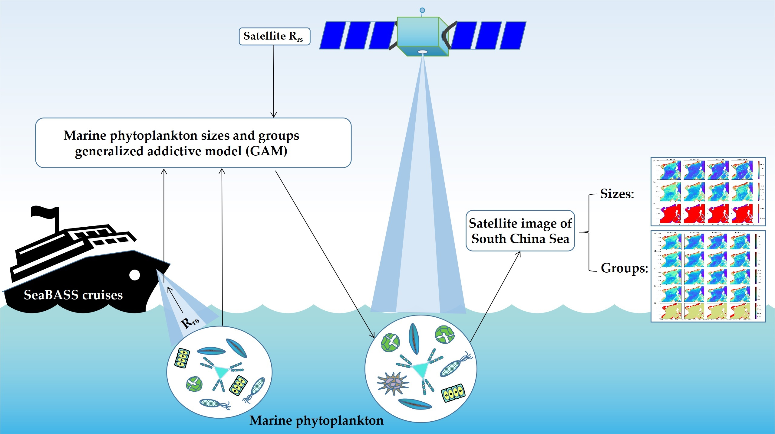
Marine phytoplankton are the basis of the whole marine ecosystem, and different groups of phytoplankton play different roles in the biogeochemical cycle. Satellite remote sensing is widely used in the retrieval of marine phytoplankton over a wide range and long time series, but not yet for taxonomical composition. In this study, we used coincident in situ measurement data from high-performance liquid chromatography (HPLC) and remote sensing reflectance (R_rs) to investigate the empirical relationships between phytoplankton groups and satellite measurements. A nonparametric model, generalized additive model (GAM), is introduced to establish inversion models of various marine phytoplankton groups. Seven inversion models (two sizes classes among the microphytoplankton and nanophytoplankton and four groups among the diatoms, dinoflagellates, chrysophytes, and cryptophytes) are applied to the South China Sea (SCS) for 2020, and satellite images of phytoplankton sizes and groups are presented. Microphytoplankton prevails in the coastal and continental shelf, and nanophytoplankton prevails in oligotrophic oceans. Among them, the dominant contribution of microphytoplankton comes from diatoms, and nanophytoplankton comes from chrysophytes. Diatoms (nearshore) and chrysophytes (outside the continental shelf) are the dominant groups in the SCS throughout the year. Dinoflagellates only become dominant in some coastal areas, while cryptophytes rarely become dominant.

1. Introduction

The ocean plays an important role in the earth’s carbon cycle, and marine phytoplankton, which uses dissolved inorganic carbon to photosynthesize organic matter, are the main primary producer in the marine ecosystem [1]. Generating approximately half of the planetary primary productivity, marine phytoplankton affects the abundance and diversity of marine organisms, drive marine energy flow and the material cycle, and promote the work of marine ecosystems [1,2,3]. In the contemporary ocean, photosynthetic carbon fixation by marine phytoplankton leads to the formation of 45 gigatons of organic carbon every year, of which 16 gigatons are exported to the ocean interior [1]. For such a huge productivity output, the variation in marine phytoplankton can affect global climate change [2,3,4].

In recent decades, the most commonly used indicator of phytoplankton biomass has been the total chlorophyll a concentration (Chl a, mg·m⁻³) [5]. However, phytoplankton often consist of hundreds of species, and different groups have different roles in biogeochemical processes (such as silicon absorption and carbon and nitrogen fixation). Thus, it is not sufficient to quantify the composition information of the phytoplankton community structure by total chlorophyll a concentration [6].

To better understand the role of different phytoplankton groups in the global carbon cycle, researchers have proposed the concept of phytoplankton functional types (PFTs) [7,8]. The division of PFTs is not necessarily related to physiological characteristics but is based on the common biogeochemical function or other characteristics of phytoplankton in the food web [9]. At present, the division of PFTs is mainly based on size class and biogeochemical function [10]. According to size class, PFTs can be partitioned into three size classes: microphytoplankton (>20 µm), nanophytoplankton (2–20 µm), and picophytoplankton (<2 µm) [11]. PFT measurements in situ can be determined by a variety of methods, including microscopy, flow cytometry, spectral fluorescence, and high-performance liquid chromatography (HPLC). Although these methods are time-consuming and laborious for field survey and sample analyses and unsuitable for continuous spatial observation, they can provide an accurate data basis on the phytoplankton composition for satellite water color remote sensing.

At present, most current knowledge of the geographical distribution and seasonal cycle of photosynthesis of marine organisms at the global scale mainly comes from satellite observations [12,13]. The algorithm based on a spectral ratio of remote sensing reflectance (R_rs) historically has been used as the default algorithm formulation to produce global chlorophyll a products from measurements made by satellite instruments [14]. In the field of ocean color remote sensing, there are two approaches to retrieve phytoplankton groups from space. One is to perform a large number of in-water radiative computations with various amounts on phytoplankton cells of different sizes. The size, shape, and pigment composition of the cells are used to simulate the inherent optical properties (IOPs) of phytoplankton and interpret their variability in the biological state of the phytoplankton population [15,16]. The other is to establish an empirical relationship between a large amount of in situ pigment data and simultaneously measured ocean water color spectrum data [12,16,17]. Compared with the in-water radiative computations approach, the empirical approach has the advantages of simple operation and quick application. As a kind of empirical approach, a generalized additive model (GAM) also can describe complex and non-linear relationship between response and predictor variables and do not require prior knowledge of the shape of the response function [3,18]. Here, we use a set of in situ HPLC data and R_rs data between 2001 and 2021 from multiple cruises of the SeaWiFS Bio-optical Archive and Storage System (SeaBASS system). Then, we introduce the nonparametric regression analysis model, GAM, to establish an empirical relationship between marine phytoplankton sizes and groups and R_rs. It explores the applicability of GAM in remote sensing inversion of marine phytoplankton sizes and groups. Furthermore, the models are applied to the South China Sea (SCS) to analyze the spatial distribution and seasonal variation of different phytoplankton groups.

2. Materials and Methods

2.1. Data Sources

High-quality in situ measurements are a prerequisite for satellite data product validation, algorithm development, and many climate-related inquiries. As such, the NASA Ocean Biology Processing Group (OBPG) maintains a repository of in situ oceanographic and atmospheric data (SeaWiFS biooptical archive and storage system, SeaBASS) to support regular scientific analyses [19,20]. The archived data of SeaBASS include measurements of apparent and inherent optical properties (AOPs & IOPs), phytoplankton pigments, and other relevant marine and atmospheric data, such as water temperature, salinity, and aerosol optical thickness. The download website of SeaBASS data is https://seabass.gsfc.nasa.gov/search_results#job_table_div (accessed on 24 May 2022).

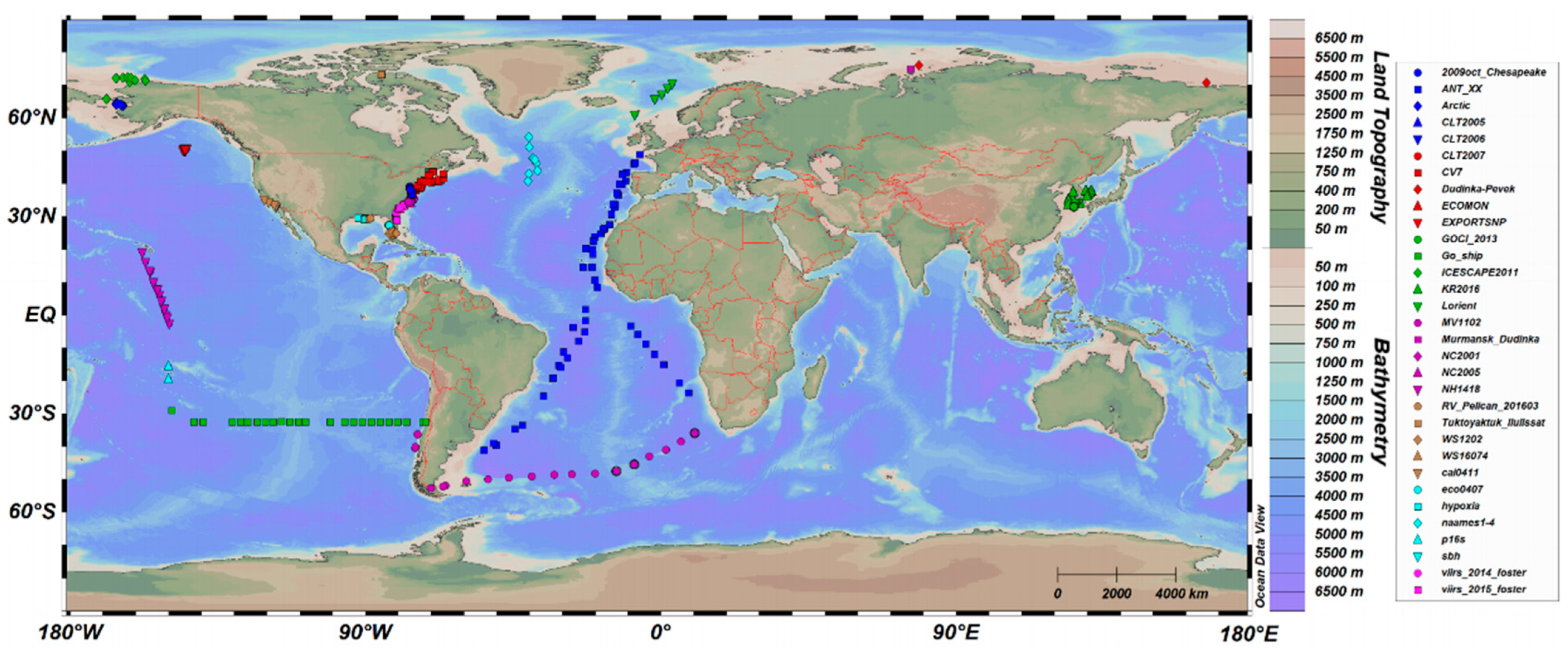
HPLC and R_rs data of the past 20 years (2001–2021) were downloaded from the SeaBASS system (https://seabass.gsfc.nasa.gov/search_results#job_table_div (accessed on 24 May 2022)). Then, 669 coincident in situ data were collected at different depths. The locations are shown in Figure 1.

Among the 669 coincident data, the time range includes 2001, 2005–2010, 2012–2014, and 2016–2017. The matching stations are mainly located in the Pacific Ocean and the Atlantic Ocean, including both Case I and Case II waters.

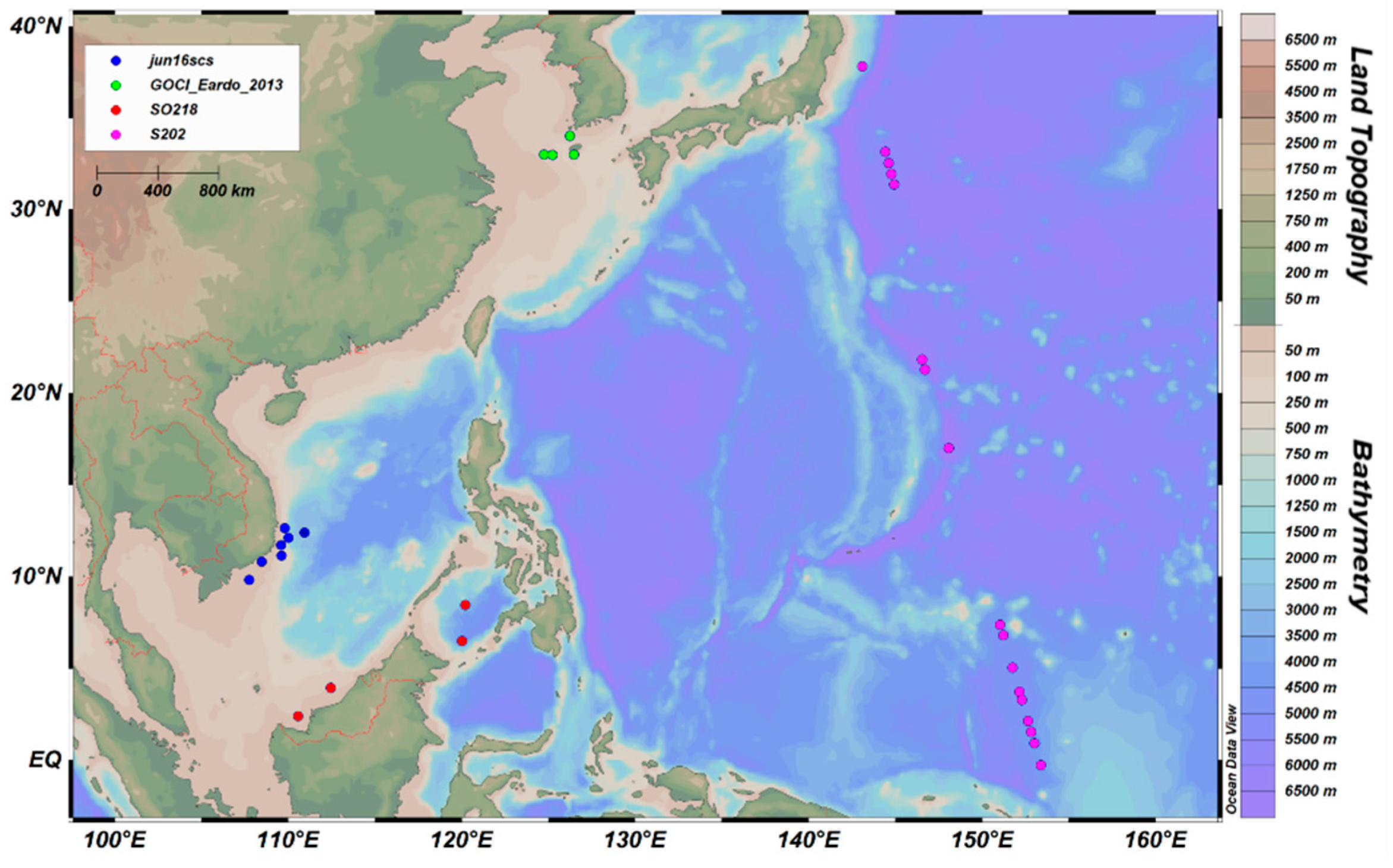
In addition, there were four cruises with HPLC data but without synchronized in situ R_rs data in the western Pacific Ocean. Therefore, Moderate Resolution Imaging Spectroradiometer (MODIS)-Terra Level 3 binned daily products with a spatial resolution of 4 km were used to obtain the synchronous R_rs at 412, 443, 488, 555, and 667 nm. The MODIS Level 3 product used in this study was atmospheric corrected by the data distributor. The atmospheric correction process removes atmospheric signal impacts. MODIS remote sensing reflectance has been validated by Zhao et al. [21]. The synchronous R_rs is coincident with these four cruises’ HPLC data. Finally, 32 coincident satellite data were selected at near-surface depths (<10 m) using the nearest method, as shown in Figure 2. The time range includes 2009, 2011, 2013, and 2016.

2.2. Phytoplankton Taxonomy from HPLC Pigments

2.2.1. Diagnostic Pigment Analysis (DPA)

Phytoplankton pigments can be divided into three categories: chlorophyll (a, b, and c), carotenoids, and phycobiliprotein (phycoerythrin, phycocyanin, and allophycocyanin). Except for chlorophyll a, a pigment ubiquitous in all phytoplankton, some pigments only exist in one or several groups. Many of these pigments are thus used as biomarker pigments of specific phytoplankton groups [22].

To identify the three size classes (Micro, Nano, and Pico) and quantify their relative proportions, Vidussi et al. [23] selected seven major pigments as diagnostic pigments (DPs) for distinct phytoplankton groups. These seven pigments are fucoxanthin (Fuco), peridinin (Perid), 19′-hexanoyloxyfucoxanthin (Hex-Fuco), 19′-butanoyloxyfucoxanthin (But-Fuco), alloxanthin (Allo), chlorophyll b (Chl b), and zeaxanthin (Zea). The proportion of the three size classes is represented by the ratio of concentrations:

[Micro] = ([Fuco] + [Perid])/DP

(1)

[Nano] = ([Hex-Fuco] + [But-Fuco] + [Allo])/DP

(2)

[Pico] = ([Chl b] + [Zea])/DP

(3)

DP = [Fuco] + [Perid] + [Hex-Fuco] + [But-Fuco] + [Allo] + [Chl b] + [Zea]

(4)

However, this is based on the fact that each taxonomic pigment has the same contribution to chlorophyll a. Obviously, this does not strictly reflect the true size of the phytoplankton communities, because some taxonomic pigments might be shared by various phytoplankton groups. Therefore, Uitz et al. [11] combined the multiple regression approach of Gieskes et al. [24] to determine the weight of seven pigments in chlorophyll a, ∑DP_w, according to

∑DP_w = 1.41 × ([Fuco] + [Perid]) + 1.27 × [Hex-Fuco] + 0.35 × [But-Fuco] + 0.6 × [Allo] + 1.01 × [Chl b] + 0.86 × [Zea]

(5)

The fractions of the chlorophyll a concentration associated with each of the three size classes are subsequently derived according to

f_Micro = 1.41 × ([Fuco] + [Perid])/∑DP_w

(6)

f_Nano = (1.27 × [Hex-Fuco] + 0.35 × [But-Fuco] + 0.6 × [Allo])/∑DP_w

(7)

f_Pico = (1.01 × [Chl b] + 0.86 × [Zea])/∑DP_w

(8)

The actual chlorophyll a concentration associated with each of three size classes is derived according to

[Micro] = f_Micro × [Chl a]

(9)

[Nano] = f_Nano × [Chl a]

(10)

[Pico] = f_Pico × [Chl a]

(11)

2.2.2. High–Performance Liquid Chromatography—CHEMical TAXonomy (HPLC-CHEMTAX)

The existence of biomarker pigments is the basis for the qualitative analysis of phytoplankton groups [22]. Some key pigments are only in one or two groups. For example, Fuco, Perid, Chl b, prasinoxanthin (Pras), zeaxanthin (Zea), and Allo are the diagnostic pigments for diatoms, dinoflagellates, chlorophyceae, prasinophyceae, cyanobacteria, and cryptophytes, respectively. However, some pigments are present in several phytoplankton groups. Overlapping pigment compositions can further complicate the quantification of phytoplankton groups [25].

Thanks to the development of statistical tools, such as CHEMTAX [26], the problem has been improved. CHEMTAX applies matrix factorization to HPLC pigment data to estimate the contribution of phytoplankton groups to Chl a. The input of the CHEMTAX program includes two matrices: one is the pigment concentrations matrix, S, obtained from HPLC data, and the other is the ratios of each phytoplankton group matrix, F. The initial matrix, F, given by a “steepest descent algorithm”, is iterated within a certain range. Finally, the optimal solution satisfying the set conditions is given to determine the composition of the phytoplankton matrix, C.

S = F × C

(12)

The initial pigment ratios of the major algal groups used in this study were obtained from the literature [26,27,28,29,30]. Eight algal groups were loaded in the CHEMTAX program: diatoms, dinoflagellates, chrysophytes, prymnesiophytes, chlorophyceae, prasinophyceae, cyanobacteria, and cryptophytes. The genus Prochlorococcus was discriminated from the other cyanobacteria based on the existence of divinyl chlorophyll a (DV Chl a). Thus, cyanobacteria in this study do not include Prochlorococcus.

2.3. Generalized Addictive Model (GAM)

In 1990, Hastie and Tibshirani [31] proposed a group of nonparametric models, generalized additive models (GAMs), which are extensions of generalized linear models (GLMs), which do not require prior knowledge of the shape of the response function. A GAM has the advantage of addressing complex nonlinear response relationships and allows one response variable to be fitted by several predictors in an additive manner [32,33]. The general equation of GAM is

$$\mathrm{g}(\mathrm{Y})=\mathsf{\epsilon }+{\sum }_{\mathrm{i}=1}^{\mathrm{n}}{\mathrm{s}}_{\mathrm{i}}\left({\mathrm{X}}_{\mathrm{i}}\right)$$

(13)

where Y is the response variable, X is the predictor, n is the number of predictors, ε is the random error term, and ${\mathrm{s}}_{\mathrm{i}}()$ is a nonparametric smooth function (it can be a smooth spline function, kernel function, or local regression smooth function).

The model uses parameters including effective degree of freedom (EDF), F statistical value, p value of the F test, generalized cross validation (GCV), adjusted R² (adj-R²), and deviance explained (DE) to describe the statistical results of the model. Among them, EDF represents the linear relationship between the response variables and predictor (EDF = 1, indicating that response variables and predictor have a linear relationship; EDF > 1, indicating a nonlinear relationship—the greater the value, the stronger the nonlinear relationship); the greater the statistical value of F, the greater the relative importance of the predictor; adj-R² and DE are the interpretation rate of model for the overall change of the response variable.

In marine science, GAMs have been used in modeling phytoplankton biomass. However, most of researchers applied GAM to freshwater lakes to explore the relationship between Chl a and environmental factors (such as temperature, salinity, nitrogen and phosphorus) [33,34,35,36]. Therefore, our study used R_rs as the predictor and established a GAM of each marine phytoplankton group to deeply explore the relationship between them. Model establishment and statistical analysis were conducted using the ‘mgcv’ package in R software version 4.1.

2.4. Statistical Approach

The model prediction accuracy was evaluated by several statistical parameters: (1) coefficient of determination (R²) calculated through 1 minus the ratio of the sum of square due to error (SSE) and the total sum of square (SST); (2) median absolute percentage error (MED); and (3) root mean squared error (RMSE)—according to Equations (14)–(18), respectively:

R² = 1 − SSE/SST

(14)

$$\mathrm{SST}={\sum }_{\mathrm{i}=1}^{\mathrm{n}}{\left({\mathrm{y}}_{\mathrm{i}}-{\mathrm{y}}_{\mathrm{i}}^{\prime }\right)}^2$$

(15)

$$\mathrm{SSE}={\sum }_{\mathrm{i}=1}^{\mathrm{n}}{\left({\mathrm{y}}_{\mathrm{i}}-\overline{\mathrm{y}}\right)}^2$$

(16)

$$\mathrm{MED}=\mathrm{Median}\left|\frac{{\mathrm{y}}_{\mathrm{i}}-{\mathrm{y}}_{\mathrm{i}}^{\prime }}{{\mathrm{y}}_{\mathrm{i}}}\right| \times 100\%$$

(17)

$$\mathrm{RMSE}=\sqrt{\frac{1}{\mathrm{n}}{\sum }_{\mathrm{i}=1}^{\mathrm{n}}{\left({\mathrm{y}}_{\mathrm{i}}-{\mathrm{y}}_{\mathrm{i}}^{\prime }\right)}^2}$$

(18)

where y_i is the true value in sample i, ${\mathrm{y}}_{\mathrm{i}}^{\prime }$ is the predicted value in sample i, and $\overline{\mathrm{y}}$ is the average of the true values.

3. Results and Discussion

3.1. Evaluation of Phytoplankton Groups

A descriptive summary of all phytoplankton groups is presented in

Table 1. Descriptive summary of the phytoplankton groups. Min and Max represent the minimum and maximum values, respectively. N is the number of samples. The unit for all groups is mg·m⁻³.

Groups	Min	Max	Mean	Median	N
Chl a	0.03000	70.21330	3.05817	0.47500	669
Micro	0.00221	52.16976	2.17843	0.19170	666
Nano	0.00334	6.66332	0.34310	0.15553	669
Pico	0.00355	15.10031	0.54641	0.11859	669
Diatoms	0.00014	36.51595	1.44788	0.16101	668
Dinoflagellates	0.00037	10.53531	0.35053	0.03609	667
Chrysophytes	0.00177	4.38621	0.26240	0.11799	667
Prymnesiophytes	0.00091	0.23894	0.01999	0.01730	168
Chlorophyceae	0.00001	0.51881	0.02215	0.00850	80
Prasinophyceae	0.00014	0.84589	0.03367	0.01568	409
Cyanobacteria	0.00257	11.80883	0.42606	0.07831	668
Cryptophytes	0.00061	11.81432	0.54931	0.05385	667

Note: Chl a = chlorophyll a; Micro = microphytoplankton; Nano = nanophytoplankton; Pico = picophytoplankton.

.

As the distribution frequency of each phytoplankton group (including Chl a, Micro, Nano, Pico, diatoms, dinoflagellates, chrysophytes, prymnesiophytes, chlorophyceae, prasinophyceae, cyanobacteria, and cryptophytes) was left-skewed, we log-transformed them to log10 to satisfy a roughly normal distribution. The normal distribution tests for each group were accomplished using density and quantile–quantile (Q–Q) plots, provided in Figure S1 (in the Supplementary Material).

3.2. Establishment of GAMs

The in situ R_rs at 412, 443, 490, 555, and 670 nm (corresponding to the SeaWiFS band setting) were used as the predictors and the in situ Chl a was used as the response variable.

The fitted GAM result for Chl a is summarized in

Table 2. Statistical summary of the fitted Chl a GAM. EDF, F, GCV, DE, and N represent the effective degrees of freedom, F statistical value, generalized cross validation, deviance explained, and number of samples, respectively (the same below).

Predictors	EDF	F	p Value	GCV	adj-R2	DE	N
Rrs412	4.240	33.422	<0.001	0.106	0.781	79.20%	669
Rrs443	6.345	22.792	<0.001
Rrs490	5.829	7.853	<0.001
Rrs555	8.377	36.488	<0.001
Rrs670	7.906	3.860	<0.001

. The Chl a GAM-fitted results show that the five predictors explained 79.2% of the total variance, with all the covariates being highly significant (p value < 0.01). The EDF value of the five predictors indicated that each of them has a nonlinear relationship with the change in Chl a. The adj-R² (0.781) and GCV (0.106 mg·m⁻³) showed that the Chl a GAM has a good fitting effect.

Similar to the Chl a GAM, the GAM was also used to fit the phytoplankton groups (Micro, Nano, Pico, diatoms, dinoflagellates, chrysophytes, prymnesiophytes, chlorophyceae, prasinophyceae, cyanobacteria and cryptophytes). The result of each fitted GAM is summarized in

Table 3. Statistical summary of the fitted Micro GAM.

Predictors	EDF	F	p Value	GCV	adj-R2	DE	N
Rrs412	3.028	21.989	<0.001	0.191	0.795	80.51%	666
Rrs443	7.353	14.825	<0.001
Rrs490	6.148	9.846	<0.001
Rrs555	8.858	33.444	<0.001
Rrs670	8.325	4.387	<0.001

,

Table 4. Statistical summary of the fitted Nano GAM.

Predictors	EDF	F	p Value	GCV	adj-R2	DE	N
Rrs412	6.985	12.086	<0.001	0.154	0.454	47.50%	669
Rrs443	4.942	11.433	<0.001
Rrs490	5.025	1.429	0.200
Rrs555	7.583	16.424	<0.001
Rrs670	1.000	1.467	0.226

,

Table 5. Statistical summary of the fitted Pico GAM.

Predictors	EDF	F	p Value	GCV	adj-R2	DE	N
Rrs412	5.639	32.896	<0.001	0.140	0.671	68.29%	669
Rrs443	6.754	27.847	<0.001
Rrs490	3.671	11.940	<0.001
Rrs555	4.235	36.468	<0.001
Rrs670	3.172	8.109	<0.001

,

Table 6. Statistical summary of the fitted diatoms GAM.

Predictors	EDF	F	p Value	GCV	adj-R2	DE	N
Rrs412	4.334	21.069	<0.001	0.167	0.803	81.35%	668
Rrs443	6.635	19.642	<0.001
Rrs490	6.334	13.590	<0.001
Rrs555	8.846	31.716	<0.001
Rrs670	7.999	3.742	<0.001

,

Table 7. Statistical summary of fitted dinoflagellates GAM.

Predictors	EDF	F	p Value	GCV	adj-R2	DE	N
Rrs412	5.034	24.350	<0.001	0.183	0.726	73.70%	667
Rrs443	6.575	20.102	<0.001
Rrs490	5.784	8.344	<0.001
Rrs555	8.522	34.915	<0.001
Rrs670	1.000	12.106	<0.001

,

Table 8. Statistical summary of the fitted chrysophytes GAM.

Predictors	EDF	F	p Value	GCV	adj-R2	DE	N
Rrs412	6.316	19.716	<0.001	0.106	0.613	62.76%	667
Rrs443	5.566	17.550	<0.001
Rrs490	5.173	3.625	0.001
Rrs555	7.793	28.675	<0.001
Rrs670	1.000	1.635	0.201

,

Table 9. Statistical summary of the fitted prymnesiophytes GAM.

Predictors	EDF	F	p Value	GCV	adj-R2	DE	N
Rrs412	1.577	0.642	0.583	0.067	0.593	62.82%	168
Rrs443	1.373	0.590	0.414
Rrs490	4.951	1.862	0.100
Rrs555	5.513	5.055	<0.001
Rrs670	1.181	0.036	0.936

,

Table 10. Statistical summary of the fitted chlorophyceae GAM.

Predictors	EDF	F	p Value	GCV	adj-R2	DE	N
Rrs412	1.000	4.695	0.034	0.540	0.208	27.19%	80
Rrs443	1.855	6.569	0.002
Rrs490	1.000	9.522	0.003
Rrs555	1.000	0.558	0.458
Rrs670	1.471	0.671	0.592

,

Table 11. Statistical summary of the fitted prasinophyceae GAM.

Predictors	EDF	F	p Value	GCV	adj-R2	DE	N
Rrs412	5.656	9.357	<0.001	0.190	0.436	48.00%	409
Rrs443	6.285	8.198	<0.001
Rrs490	8.148	4.663	<0.001
Rrs555	7.792	6.219	<0.001
Rrs670	3.788	2.412	0.039

,

Table 12. Statistical summary of the fitted cyanobacteria GAM.

Predictors	EDF	F	p Value	GCV	adj-R2	DE	N
Rrs412	5.183	38.564	<0.001	0.122	0.749	75.78%	668
Rrs443	7.478	29.685	<0.001
Rrs490	5.680	9.820	<0.001
Rrs555	3.036	67.767	<0.001
Rrs670	2.490	24.344	<0.001

and

Table 13. Statistical summary of the fitted cryptophytes GAM.

Predictors	EDF	F	p Value	GCV	adj-R2	DE	N
Rrs412	4.941	21.939	<0.001	0.167	0.761	77.09%	667
Rrs443	5.877	21.254	<0.001
Rrs490	5.963	10.505	<0.001
Rrs555	8.688	36.253	<0.001
Rrs670	1.000	12.602	<0.001

.

In the establishment of models, except for Nano, Chlorophyceae, and prasinophyceae, the deviance explained by the chlorophyll a, Micro, Pico, diatoms, dinoflagellates, chrysophytes, prymnesiophytes, cyanobacteria, and cryptophytes fitted model is more than 60%.

The different cell sizes of the phytoplankton present different spectral features, including their absorption and backscattering properties in a wide band range from 400 to 700 nm. This difference in the absorption and backscattering induces the variability in spectral shape of remote sensing reflectance [37]. Li et al. [17] found that the spectral features with particular importance around 440–555 nm have a significant response to phytoplankton size. Brewin et al. [38] found there are contrasting spectral shapes between the three phytoplankton sizes in the green part of the spectrum (500–600 nm). It is consistent with our results that R_rs555 has a significant response to micro-, nano- and picophytoplankton concentrations (the F value is high in Table 3, Table 4 and Table 5). R_rs412, R_rs443, and R_rs555 have a significant contribution for estimation of all three sizes’ concentration. In addition, Brewin et al. [38] also demonstrated that nanophytoplankton has a distinct absorption at ~450 nm. In our study, the nanophytoplankton GAM (adj-R² = 0.454) is a little worse than the pico- and microphytoplankton model (adj-R² = 0.671 and adj-R² = 0.795). R_rs412, R_rs443, and R_rs555 contribute significantly in estimating the nanophytoplankton concentration, while R_rs490 and R_rs670 have a limited contribution to nanophytoplankton estimation (Table 4). In the blue-green part of the spectrum (400–600 nm), R_rs490 has a lower contribution to the phytoplankton size GAM compared with other spectral bands, especially for the nanophytoplankton retrieval model. Sun et al. [39] applied remote sensing reflectance at 488 nm and 555 nm to obtain the phytoplankton size. They found that the microphytoplankton retrievals show a greater sensitivity than that of the nano- and picophytoplankton on R_rs488 or R_rs555. In the red part of the spectrum, Roy et al. [40] developed a semi-analytical algorithm based on phytoplankton absorption features at a red wavelength (676 nm) to obtain the phytoplankton size distribution. However, our results illustrate that R_rs670 have the smallest (not significant) contribution to the micro-, nano- and picophytoplankton retrieval estimation.

Satellites detect some phytoplankton species (such as cyanobacteria, diatoms, dinoflagellates, etc.) with a similar chlorophyll biomass, provided they have contrasting optical signatures. Some studies demonstrated that satellite spectra have a distinct response for cyanobacteria and diatoms [41,42]. Isada et al. [43] found that diatom and cyanobacteria have differences in absorption in the green-red part of the spectrum. The diatoms absorption normalized at 443 nm is higher in the green-red part of the spectrum than that of cyanobacteria, resulting in lower remote sensing reflectance for diatoms. Our results demonstrate that the contribution of R_rs(670) to the diatom model is lower than that for cyanobacteria (Table 6 and Table 12). Aguirre-Gomez et al. [44] also indicated that cyanobacteria has a more obvious optical signal at ~670 nm than diatoms. Stuart et al. [45] found that the absorption at 443 and 490 nm normalized at 555 nm is significantly lower for the diatom-dominated population than for the prymnesiophyte-rich population, indicating that there are larger R_rs443 and R_rs490 for the diatom-dominated population. The prymnesiophytes GAM model developed in this study is mainly contributed by R_rs490 and R_rs555. It was thought that diatoms and dinoflagellates contain some of the same pigments, and therefore their light absorption features are similar [46]; however, their optical backscattering features are different due to their structure difference. Discriminating between these two groups depends on the variability in the R_rs spectral shape induced by backscattering [47]. In fact, there are some difference in the absorption between these two groups. The absorption peak of the dinoflagellates at ~440 nm is steeper than that of diatoms. In the case of absorption peaks of the same magnitude, the absorption curve of dinoflagellates drops faster at ~490 nm. It is also found that dinoflagellates have a stronger absorption at ~670 nm [48]. Our results indicate that, compared with diatoms, the contribution of R_rs490 for the dinoflagellates model decreases and the contribution of R_rs670 increases (Table 6 and Table 7). Based on the steeper absorption peak characteristics of the dinoflagellates, Bracher et al. [49] also retrieved cyanobacteria and diatoms based on their spectral variability within 429–495 nm. Sadeghi et al. [50] retrieved diatoms, coccolithophores, and dinoflagellates based on a spectral absorption difference over the 429–521 nm spectral range. Relatively little research has been done on remote sensing of chrysophytes and cryptophytes. In this study, their retrieval accuracy performs well. R_rs412, R_rs443, and R_rs555 have larger contributions for chrysophytes estimation (Table 8). R_rs at all five bands demonstrate a more near-equivalent contribution for cryptophytes estimation (Table 13). Compared to other species models, the contribution of R_rs at 490 and 670 nm also increases.

To test the effectiveness of the GAM, we used random sampling to extract 70% of the data as the training data set and the remaining 30% of the data as the test data set and randomly cycle 1000 times to test the prediction accuracy. This helps to test whether our models are effective or an effect caused by the randomness of the data set. We take the root mean squared error (RMSE), median absolute percentage error (MED), and coefficient of determination (R²) as the indicators of the models’ prediction accuracy.

From the training results of various phytoplankton GAM (

Table 14. Training results of the GAM. Note: RMSE, MED, R², and N represent the root mean squared error, median absolute percentage error, coefficient of determination, and number of samples, respectively. The adjusted R² statistic can take on any value less than or equal to 1, with a value closer to 1 indicating a better fit. Negative values can occur when the model contains terms that do not help to predict the response.

GAM	RMSE	MED	R2	N
Chl a	0.3578	35.76%	0.688	201
Micro	0.5042	32.54%	0.666	200
Nano	0.4071	22.67%	0.379	201
Pico	0.3817	25.14%	0.642	201
Diatoms	0.4768	31.42%	0.667	201
Dinoflagellates	0.4689	16.21%	0.563	201
Chrysophytes	0.3425	18.26%	0.540	201
Prymnesiophytes	0.2900	8.65%	0.403	51
Chlorophyceae	0.8111	21.73%	−0.273	24
Prasinophyceae	0.4568	14.49%	0.311	123
Cyanobacteria	0.3627	20.51%	0.715	201
Cryptophytes	0.4491	19.55%	0.683	201

), eight GAM models achieve a good fitted effect (R² > 0.5). They are chlorophyll a, Micro, Pico, diatoms, dinoflagellates, chrysophytes, cyanobacteria, and cryptophytes models. The prymnesiophytes model performs a little worse than the above eight models with an R² of 0.403. The correlation coefficient is relatively small for the Nano, chlorophyceae, and prasinophyceae models.

In addition, the GAM of the various marine phytoplankton groups studied and developed in this paper was constructed based on different depths. Therefore, theoretically, as long as the R_rs data at different depths can be accurately obtained, the distribution information of the phytoplankton groups in the research area can be estimated by using the marine phytoplankton group GAM developed in this study, whether it is surface or deep water [51].

3.3. Comparison between GAMs and Other Algorithms

In addition to the training models, the GAM models are also compared with other inversion algorithms. The empirical ocean chlorophyll (OC) algorithm from O’Reilly et al. [52] is the current default chlorophyll a algorithm for SeaWiFS and MODIS. The OC algorithm is a fourth-order polynomial calculated using an empirical relationship derived from in situ measurements of Chl a and R_rs in the blue-to-green region of the visible spectrum.

$${\log }_{10}\mathrm{Chl} \mathrm{a}={\mathrm{a}}_0+{\sum }_{\mathrm{i}=1}^{\mathrm{n}}{\mathrm{a}}_{\mathrm{i}}\left({\log }_{10}\left({\mathrm{R}}_{\mathrm{rs}\left(\mathsf{\lambda }\mathrm{blue}\right)}/{\mathrm{R}}_{\left(\mathrm{rs}\mathsf{\lambda }\mathrm{green}\right)}\right)\right)$$

(19)

where a₀–a₄ are the empirical regression coefficients, for which the current values of OC4v6 (the ocean chlorophyll 4 algorithm vision 6) are 0.3272, 2.9940, 2.7218, 1.2259, and 0.5683, respectively.

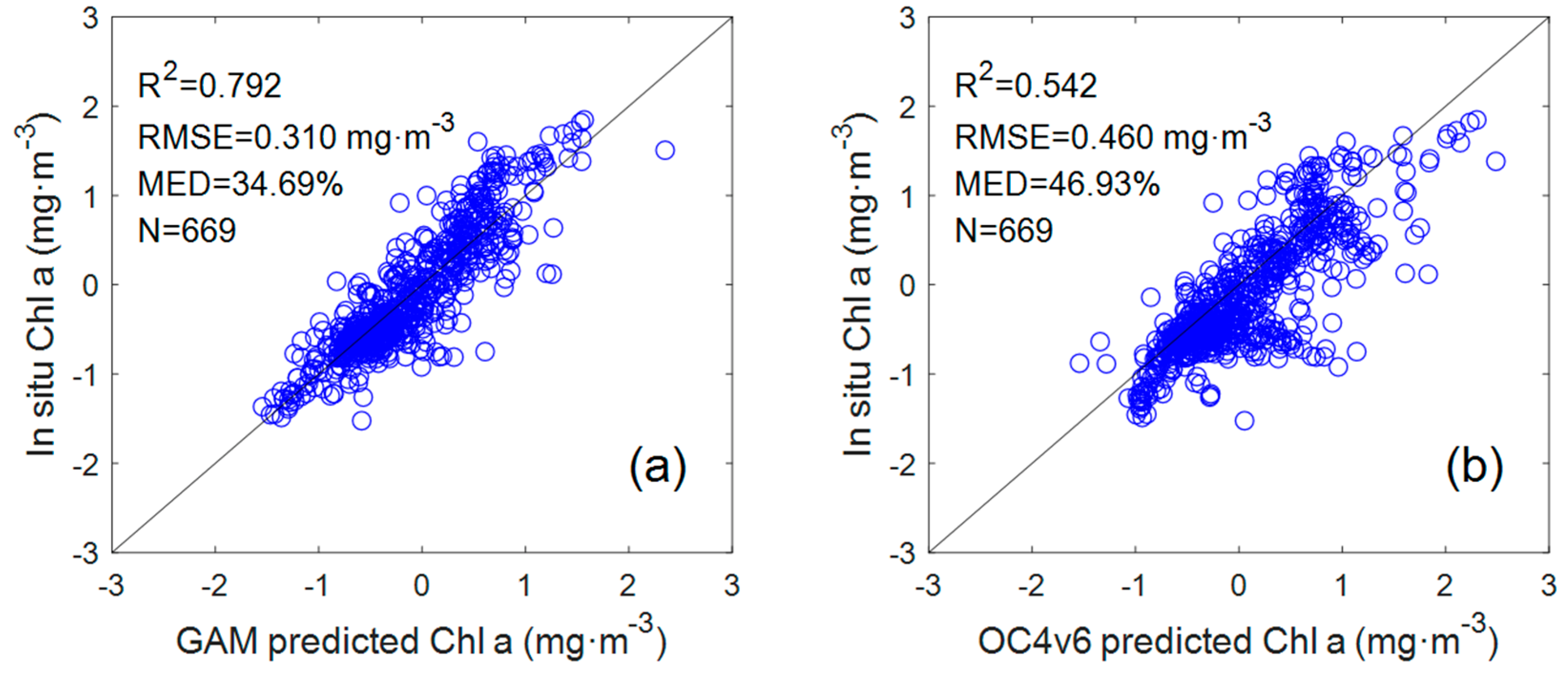
To compare with the GAM, the data set used for the OC4v6 algorithm was also taken from 669 coincident in situ data points corresponding to the GAM. From the comparison results of the Chl a GAM and OC4v6 algorithms (Figure 3), it can be seen that the OC4v6-retrieved Chl a showed a lower coefficient of determination (R² = 0.542, n = 669) and higher RMSE and MED from the in situ Chl a (RMSE = 0.46 mg·m⁻³, MED = 46.93%). Indeed, as the current default chlorophyll a algorithm, the OC algorithm has achieved acceptable inversion results in most Case I waters, but it has limitations in some areas, such as coastal waters with complex optical characteristics. The data set in this study was collected in both Case I waters and coastal waters, which may be the reason for the poor performance of the OC algorithm.

Similar to the OC algorithm, Pan et al. [25] adopted a set of third-order polynomial functions to develop algorithms for individual pigment concentrations from R_rs ratios:

log(Pigment) = A₀ + A₁X + A₂X² + A₃X³

(20)

X = log(R_rs490/R_rs555) or X = log(R_rs490/R_rs670)

(21)

where A₀–A₃ are the empirical regression coefficients.

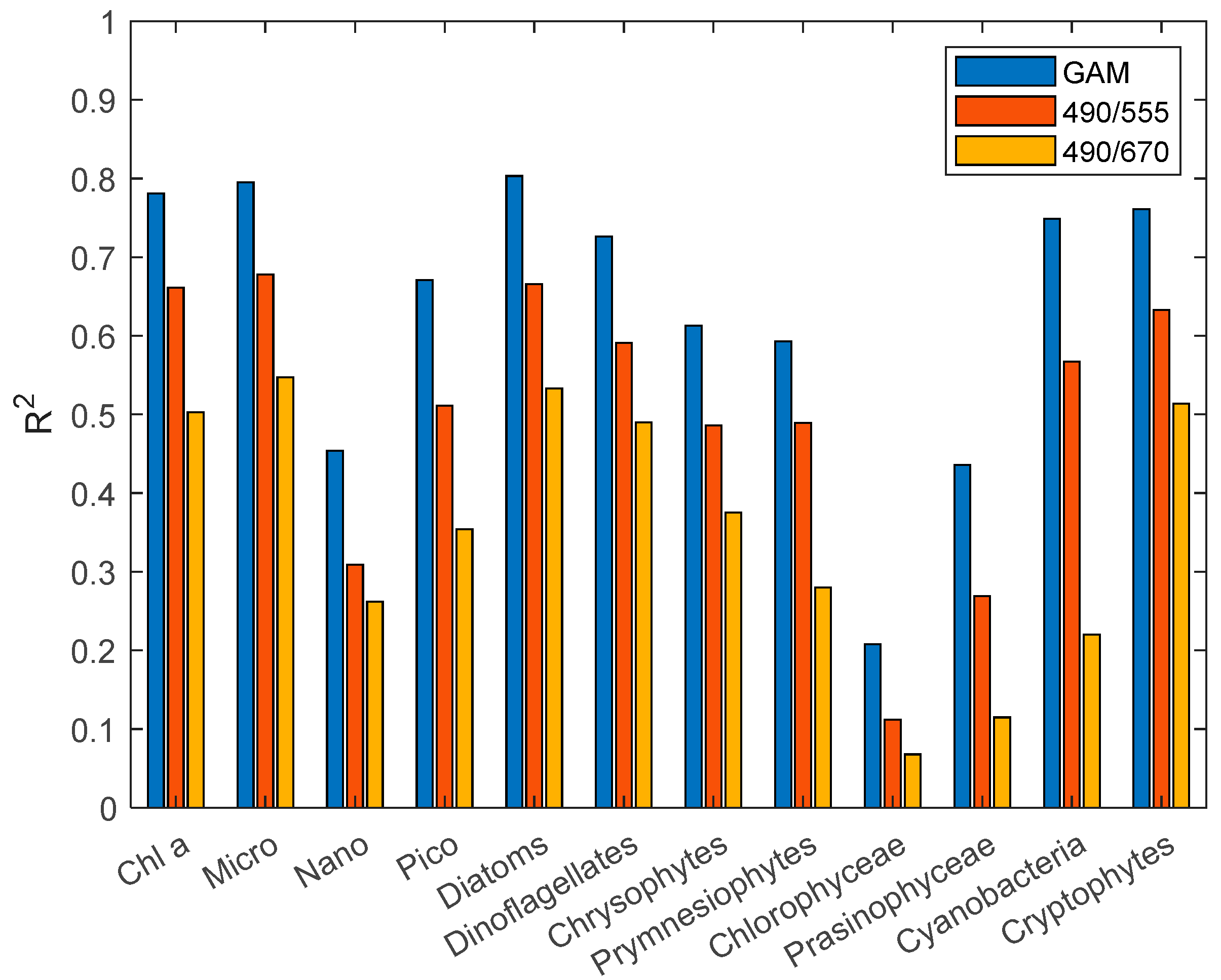
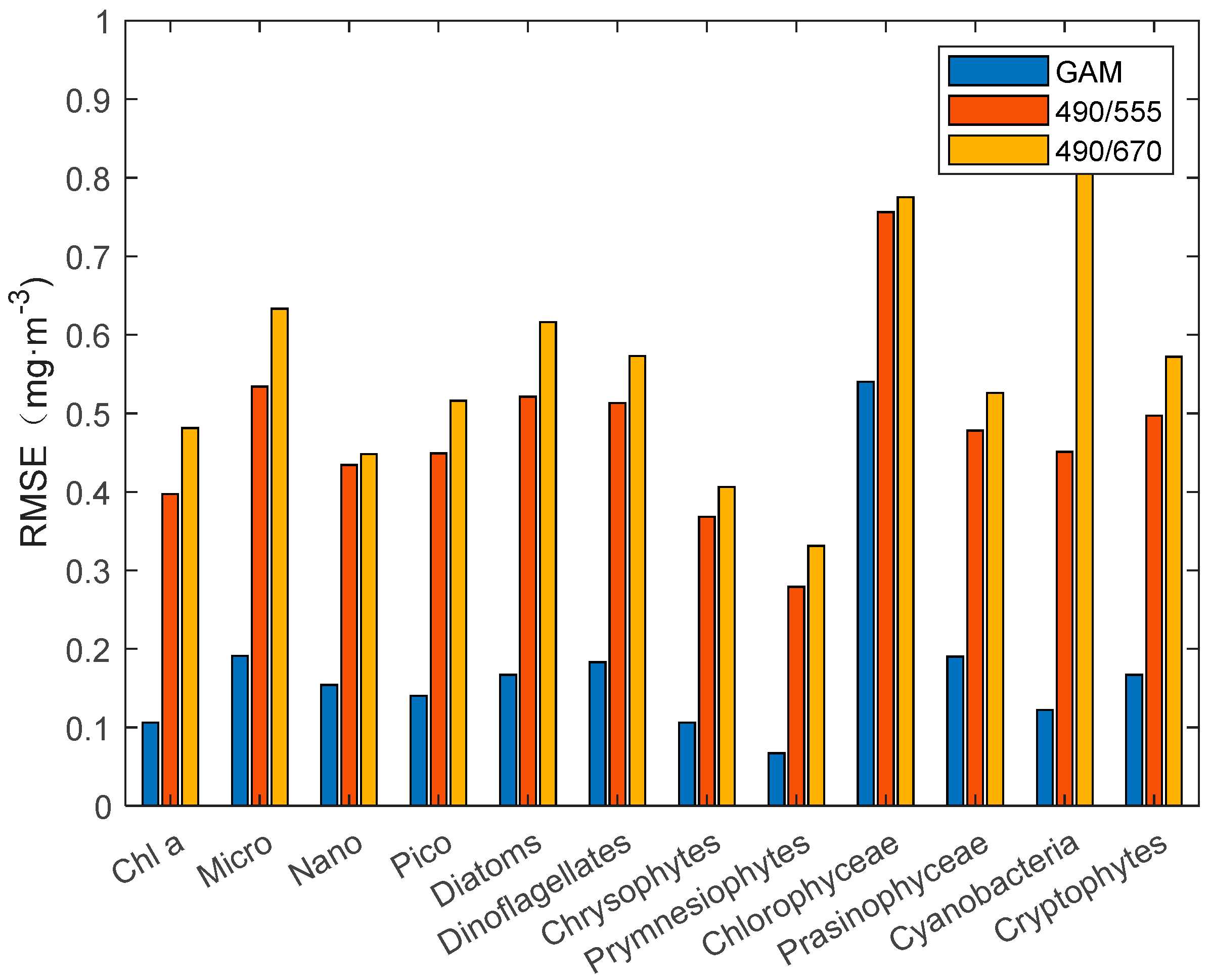
Therefore, similar to O’Reilly et al. [52] and Pan et al. [25], we constructed a third-order polynomial algorithm for individual groups of phytoplankton. The statistical results (Figure 4 and Figure 5) of R² and RMSE show that the third-order polynomial algorithm based on the R_rs490/R_rs555 band ratio is better than the R_rs490/R_rs670 band ratio. In the comparison results between the GAM and third-order polynomial algorithm, the GAM performs better than the third-order polynomial algorithm, with a higher R² and lower RMSE. The RMSE of the third-order polynomial algorithm generally exceeds 0.3 mg·m⁻³. In addition, the poor performance (R² < 0.5) of the Nano, chlorophyceae, and prasinophyceae models can be seen concisely and clearly from Figure 4 and Figure 5.

3.4. Model Evaluation Using Satellite Data

In Section 3.2, we established the GAM of the marine phytoplankton groups using in situ data, and obtained nine models with good performance, namely, chlorophyll a, Micro, Pico, diatoms, dinoflagellates, chrysophytes, prymnesiophytes, cyanobacteria, and cryptophytes. In addition, although the R² of the Nano model is only 0.454, it is also included in the scope of the discussion in this section. In Section 2.1, we mentioned that there are four cruises without in situ R_rs data matching the HPLC data in the western Pacific Ocean. Therefore, these four cruises (a total of 32 coincident satellite data) independent of the construction GAM data are very suitable for evaluating the performance of the GAM in remote sensing satellites.

Ten models were applied to the ocean color satellite Level 3 binned R_rs products of MODIS-Terra, and the derived values were compared with the in situ data. R_rs488 and R_rs667 in MODIS were assumed to be equal to their values at 490 and 670 nm (SeaWiFS band setting).

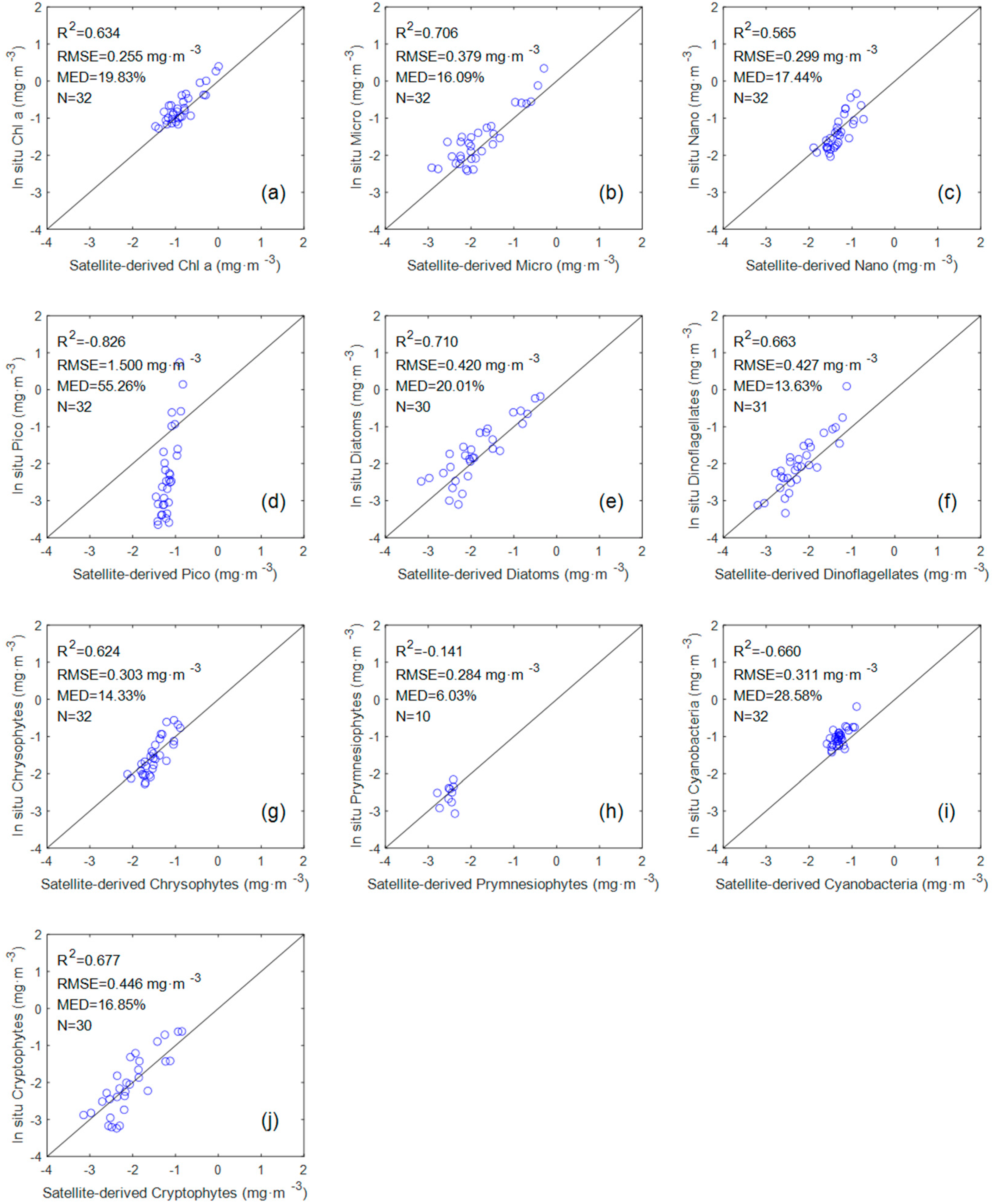
The evaluation results (Figure 6) of seven groups (Chl a, Micro, Nano, diatoms, dinoflagellates, chrysophytes, and cryptophytes) showed a good tendency towards accuracy (R² > 0.5 and MED < 20%). However, the evaluation results of Pico, premnesiophytes, and cyanobacteria exhibit dispersion and poor statistical correlation. The R² value of the three groups are −0.826, −0.141, and −0.66, respectively. A negative value of R² indicates that the sum of squares of errors (SSE) in the predicted value of the model is much greater than the sum of squares of the total deviations (SST). We are surprised by the performance of the Pico and cyanobacteria models in this comparison, because they perform well in the previous in situ measurements.

3.5. Application of GAMs in the South China Sea

The seven models with good performance in Section 3.4 were applied to the SCS, to obtain the spatial–temporal distribution and seasonal variation map of each phytoplankton group in 2020. Among them, December to February is winter, March to May is spring, June to August is summer, and September to November is autumn.

The open deep basin of the South China Sea is characterized as an oligotrophic water type, which is similar with that of the oligotrophic western Pacific water. Furthermore, the seawater in the coastal area of the South China Sea has the typical optical complex water characteristics of the coastal waters in China. According to the results of the dominant optical water class by Jackson et al. [53], the central deep basin of the South China Sea has the same optical water class as the lower and middle latitude waters of the western Pacific. Coastal water of the South China Sea has the same optical water class as some areas of the Yellow River region of China. In addition, due to the water exchange between the western Pacific and the South China Sea, the distribution and concentration of the algae type in the western Pacific Ocean are closely related to that of the South China Sea [54].

Figure 7 shows that the Chl a abundance generally decrease from the inner shelf to outer shelf and the higher abundance in the inner shelf is strongly influenced by river discharge (e.g., Pearl River, Red River, and Mekong River). The shallow water depths near the shore and the rich nutrient supplements are very suitable for the growth and reproduction of phytoplankton [55]. Higher Chl a abundance in the winter relative to the summer are consistent with a previous study in the SCS [56]. The higher abundance of Chl a are associated with lower temperature and higher nutrients, and temperature and nutrients are usually the limiting factors for phytoplankton growth [22]. In winter and spring, Figure 7 clearly shows that there is a high abundance of chlorophyll in the southwestern Taiwan Strait, northern Luzon Island, and western Hainan Island, with an average concentration of 1 mg·m⁻³. There is a strong northeast monsoon prevailing in the SCS from October to April, which makes the seawater offshore Ekman transport in these areas, causing the upwelling of low-temperature and high-nutrient seawater from the bottom. The violent agitation of the monsoon also enhances the vertical mixing of seawater, resulting in high chlorophyll levels in the SCS in winter and spring. In summer, the southwest monsoon prevailing in the SCS leads to the emergence of upwelling areas along the coast of Guangdong, the east of Hainan Island, and Vietnam. In addition, in eastern Vietnam, approximately 12°N usually forms a chlorophyll belt from the upwelling of Vietnam to the SCS basin. This is because an offshore jet from southwest to northeast is formed between the cold and warm eddies to transport the cold-water mass generated in the upwelling area to the SCS basin [57,58,59].

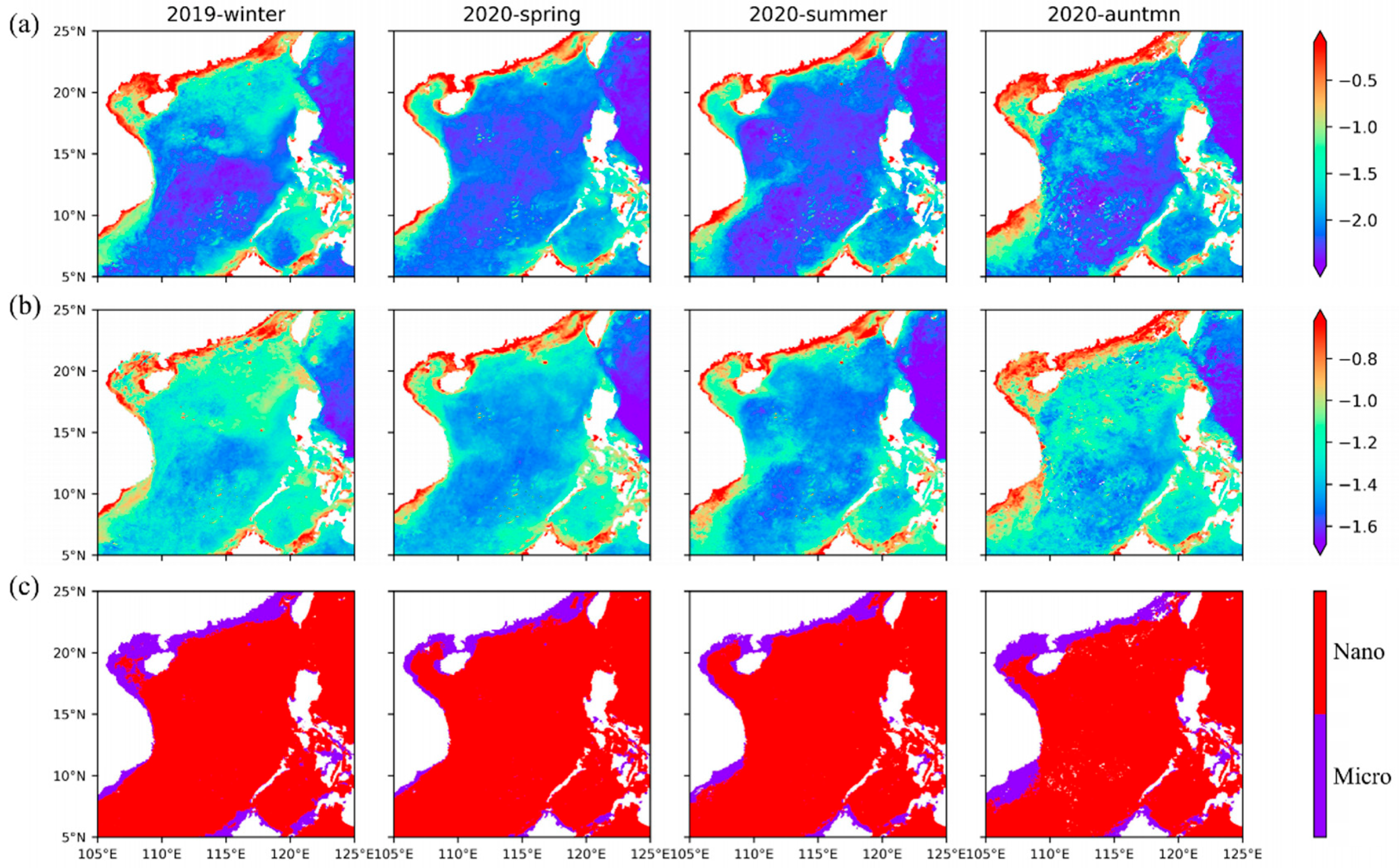
Among the two size classes retrieved by our model, both Micro (Figure 8a) and Nano (Figure 8b) show the distribution characteristics of high abundance in winter and low abundance in summer. The distribution map of the dominant group (Figure 8c) shows well-defined and persistent large-scale structures characterized to the first order by the dominance of Nano in oligotrophic waters; the average concentration reached 0.1 mg·m⁻³, whereas Micro prevails in the coastal and continental shelf, and the average concentration reaches 0.5 mg·m⁻³. The main groups of Micro are diatoms and dinoflagellates, which generally occupy an absolute advantage in the nearshore [60]. These patterns are consistent with the expected nutrient conditions in these regions, as diatoms are favored under more nutrient-replete conditions, while Nano is favored in nutrient-depleted water [22,61]. The higher efficiency of nutrient utilization due to their small size (higher surface-to-volume ratio) permits Nano to grow faster than Micro in nutrient-poor waters [25]. These results are also consistent with those estimated from field samples [30,62]. In addition, it is also indicated that turbid coastal water conditions with limited light intensity may stimulate the growth of microphytoplankton, possibly due to large superficial areas of these large-sized algal particles that possess stronger light availability than small one [63,64]. The small-sized nanophytoplankton growth would be suppressed by the turbid coastal water.

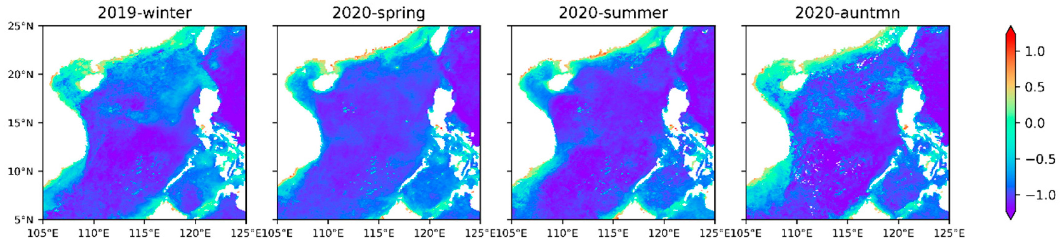
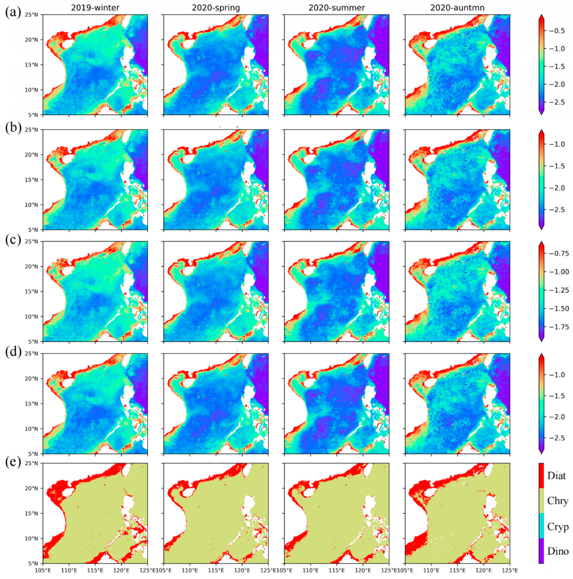
Among the four groups retrieved by our model, the four groups show the characteristics of a gradually decreasing abundance from winter to summer, especially in the open ocean, while the abundance of the four groups increased toward the coast. Among them, diatoms (Figure 9a) are mainly distributed in the nearshore, and the average concentration can reach 0.3 mg·m⁻³. Indeed, silicate is very important for the growth of diatoms, and the rivers bring abundant silicate to the nearshore [65]. In addition, the distribution range of diatoms gradually decreases from winter to summer, but diatoms are still common in the upwelling area year-round, and the concentration is greater than 0.1 mg·m⁻³. Dinoflagellates (Figure 9b) also mainly occur in the nearshore area with abundant nutrients, with an average concentration of approximately 0.1 mg·m⁻³ and approximately 0.03 mg·m⁻³ in the upwelling area. Aiken et al. [66] also found the diatom and dinoflagellate populations are located in shallow water or upwelled water. Nanophytoplankton chrysophytes (Figure 9c) and cryptophytes (Figure 9d) also have a high abundance in the oligotrophic ocean in summer, with average concentrations of approximately 0.025 mg·m⁻³ and 0.01 mg·m⁻³, respectively. In autumn and winter, the average concentrations reached 0.063 mg·m⁻³ and 0.031 mg·m⁻³, respectively. In the seasonal upwelling area, the average concentrations of chrysophytes and cryptophytes can reach 0.158 mg·m⁻³ and 0.056 mg·m⁻³, respectively.

The distribution map of the dominant groups (Figure 9e) shows that diatoms (nearshore) and chrysophytes (outside the continental shelf) are the dominant groups in the SCS throughout the year. Dinoflagellates only become dominant in some coastal areas, but compared with diatoms, dinoflagellates have a limited dominant range. Among the four groups, cryptophytes rarely become the dominant group in the SCS. Compared with the chrysophytes, cryptophytes contribute less to Nano, but the sum of their abundance makes individual areas dominated by Micro change to Nano. Combined with the dominant groups of Micro and Nano, it can be seen that the main contribution of Micro comes from diatoms, while Nano comes from chrysophytes. The suitable growth conditions near the shore make the groups with large size classes, such as diatoms and dinoflagellates, dominant, while nanophytoplankton, such as chrysophytes and cryptophytes, are dominant offshore, where there are fewer nutrients. In addition, a clear seasonal cycle is also evidenced west of Hainan Island, where chrysophytes dominate in summer and large-scale diatom blooms occur in winter. These consistencies validate our inversion models proposed in this study for estimating the phytoplankton sizes and groups from satellite remote sensing.

The satellite retrievals of phytoplankton sizes and groups using our empirical models were relatively successful. However, some models show instability in the process of training the models and evaluation using satellite data. This instability might be partly explained by the differences in the dynamic range of the measured data (spatial mismatch exists between in situ and satellite data) or because there was not enough matching data [67]. In addition, there might be some possible sources of uncertainty: (1) we assumed R_rs488 and R_rs667 to be equal to R_rs490 and R_rs670; and (2) we quantified the phytoplankton composition and abundance by using the proposed modified classification (DPA and HPLC-CHEMTAX). The regression coefficient in DPA comes from the regression results in the ocean pigment data, and CHEMTAX also depends on the initial input pigment ratio. These factors may have induced the deviations in our models.

4. Conclusions

We used coincident in situ measurement data from HPLC and R_rs to investigate the empirical relationships between phytoplankton groups and satellite measurements. A nonparametric model, GAM, was introduced to establish inversion models of various marine phytoplankton groups. Nine models performed well based on the in situ data. Among them, seven models were relatively stable in satellite remote sensing inversion. Therefore, we only used these seven models (two size classes among the microphytoplankton and nanophytoplankton and four groups among the diatoms, dinoflagellates, chrysophytes, and cryptophytes) to retrieve the phytoplankton groups in the South China Sea. The results indicate that microphytoplankton prevails in the coastal and continental shelf, and nanophytoplankton prevails in the oligotrophic oceans. Among them, the dominant contribution to microphytoplankton comes from diatoms, and for nanophytoplankton from chrysophytes. Among the four groups retrieved by our model, diatoms (nearshore) and chrysophytes (outside the continental shelf) are the dominant groups in the SCS throughout the year. Dinoflagellates only become dominant in some coastal areas while cryptophytes rarely become dominant. These results are spatially coherent and consistent with the current knowledge of this region in terms of both phytoplankton abundance and distribution.

References

- Falkowski, P.G.; Barber, R.T.; Smetacek, V.V. Biogeochemical controls and feedbacks on ocean primary production. Science 1998, 281, 200–207. [Google Scholar] [CrossRef] [Green Version]
- Field, C.B.; Behrenfeld, M.J.; Randerson, J.T.; Falkowski, P. Primary production of the biosphere: Integrating terrestrial and oceanic components. Science 1998, 281, 237–240. [Google Scholar] [CrossRef] [PubMed] [Green Version]
- Boyce, D.G.; Lewis, M.R.; Worm, B. Global phytoplankton decline over the past century. Nature 2010, 466, 591–596. [Google Scholar] [CrossRef] [PubMed]
- Azam, F.; Malfatti, F. Microbial structuring of marine ecosystems. Nat. Rev. Microbiol. 2007, 5, 782–791. [Google Scholar] [CrossRef] [PubMed]
- Siegel, D.A.; Behrenfeld, M.; Maritorena, S.; McClain, C.R.; Antoine, D.; Bailey, S.W.; Bontempi, P.S.; Boss, E.S.; Dierssen, H.M.; Doney, S.C.; et al. Regional to global assessments of phytoplankton dynamics from the SeaWiFS mission. Remote Sens. Environ. 2013, 135, 77–91. [Google Scholar] [CrossRef] [Green Version]
- Kostadinov, T.S.; Milutinovic, S.; Marinov, I.; Cabre, A. Carbon-based phytoplankton size classes retrieved via ocean color estimates of the particle size distribution. Ocean Sci. 2016, 12, 561–575. [Google Scholar] [CrossRef] [Green Version]
- Reynolds, C.S.; Huszar, V.; Kruk, C.; Naselli-Flores, L.; Melo, S. Towards a functional classification of the freshwater phytoplankton. J. Plankton Res. 2002, 24, 417–428. [Google Scholar] [CrossRef]
- Weithoff, G. The concepts of ‘plant functional types’ and ‘functional diversity’ in lake phytoplankton-a new understanding of phytoplankton ecology? Freshw. Biol. 2003, 48, 1669–1675. [Google Scholar] [CrossRef]
- Nair, A.; Sathyendranath, S.; Platt, T.; Morales, J.; Stuart, V.; Forget, M.H.; Devred, E.; Bouman, H. Remote sensing of phytoplankton functional types. Remote Sens. Environ. 2008, 112, 3366–3375. [Google Scholar] [CrossRef]
- Mouw, C.B.; Hardman-Mountford, N.J.; Alvain, S.; Bracher, A.; Brewin, R.J.W.; Bricaud, A.; Ciotti, A.M.; Devred, E.; Fujiwara, A.; Hirata, T.; et al. A consumer’s guide to satellite remote sensing of multiple phytoplankton groups in the global ocean. Front. Mar. Sci. 2017, 4, 1–19. [Google Scholar] [CrossRef] [Green Version]
- Uitz, J.; Claustre, H.; Morel, A.; Hooker, S.B. Vertical distribution of phytoplankton communities in open ocean: An assessment based on surface chlorophyll. J. Geophys. Earth Surf. 2006, 111, 1–23. [Google Scholar] [CrossRef]
- Alvain, S.; Moulin, C.; Dandonneau, Y.; Breon, F.M. Remote sensing of phytoplankton groups in case 1 waters from global SeaWiFS imagery. Deep Sea Res. Part I Oceanogr. Res. Pap. 2005, 52, 1989–2004. [Google Scholar] [CrossRef] [Green Version]
- Alvain, S.; Moulin, C.; Dandonneau, Y.; Loisel, H. Seasonal distribution and succession of dominant phytoplankton groups in the global ocean: A satellite view. Glob. Biogeochem. Cycles 2008, 22, 1–15. [Google Scholar] [CrossRef]
- Hu, C.; Lee, Z.; Franz, B. Chlorophyll aalgorithms for oligotrophic oceans: A novel approach based on three-band reflectance difference. J. Geophys. Res. Ocean. 2012, 117, 1–25. [Google Scholar] [CrossRef] [Green Version]
- Stramski, D.; Bricaud, A.; Morel, A. Modeling the inherent optical properties of the ocean based on the detailed composition of the planktonic community. Appl. Opt. 2001, 40, 2929–2945. [Google Scholar] [CrossRef] [PubMed]
- Loisel, H.; Nicolas, J.M.; Deschamps, P.Y.; Frouin, R. Seasonal and inter-annual variability of particulate organic matter in the global ocean. Geophys. Res. Lett. 2002, 29, 2196–2200. [Google Scholar] [CrossRef]
- Li, Z.; Li, L.; Song, K.; Cassar, N. Estimation of phytoplankton size fractions based on spectral features of remote sensing ocean color data. J. Geophys. Res. Ocean. 2013, 118, 1445–1458. [Google Scholar] [CrossRef]
- Matus-Hernández, M.Á.; Martínez-Rincón, R.O.; Aviña-Hernández, R.J.; Hernández-Saavedra, N.Y. Landsat-derived environmental factors to describe habitat preferences and spatiotemporal distribution of phytoplankton. Ecol. Model. 2019, 408, 1–9. [Google Scholar] [CrossRef]
- Werdell, P.J.; Fargion, G.S.; Mcclain, C.R.; Bailey, S.W. The seaWiFS bio-optical archive and storage system (SeaBASS): Current architecture and implementation. NASA Tech. 2002, 48, 1–45. [Google Scholar]
- Werdell, P.J.; Bailey, S.; Fargion, G.; Pietras, C.; Mcclain, C. Unique data repository facilitates ocean color satellite validation. Eos. Trans. Am. Geophys. Union 2003, 84, 377–392. [Google Scholar] [CrossRef]
- Zhao, W.J.; Wang, G.Q.; Cao, W.X.; Cui, T.W.; Wang, G.F.; Ling, J.F.; Sun, L.; Zhou, W.; Sun, Z.H.; Xu, Z.T.; et al. Assessment of SeaWiFS, MODIS, and MERIS ocean colour products in the South China sea. Int. J. Remote Sens. 2014, 35, 4252–4274. [Google Scholar] [CrossRef]
- Jeffrey, S.; Vesk, M. Introduction to marine phytoplankton and their pigment signatures. Phytoplankton Pigment. Oceanogr. 1997, 10, 407–428. [Google Scholar]
- Vidussi, F.; Claustre, H.; Manca, B.B.; Luchetta, A.; Marty, J.C. Phytoplankton pigment distribution in relation to upper thermocline circulation in the eastern Mediterranean Sea during winter. J. Geophys. Res. Earth Surf. 2001, 106, 19939–19956. [Google Scholar] [CrossRef]
- Gieskes, W.; Kraay, G.W.; Nontji, A.; Setiapermana, D. Monsoonal alternation of a mixed and a layered structure in the phytoplankton of the euphotic zone of the banda sea (Indonesia): A mathematical analysis of algal pigment fingerprints. Neth. J. Sea Res. 1988, 22, 123–137. [Google Scholar] [CrossRef]
- Pan, X.J.; Mannino, A.; Russ, M.E.; Hooker, S.B.; Harding, L.W. Remote sensing of phytoplankton pigment distribution in the United States northeast coast. Remote Sens. Environ. 2010, 114, 2403–2416. [Google Scholar] [CrossRef] [Green Version]
- Mackey, M.D.; Mackey, D.J.; Higgins, H.W.; Wright, S.W. CHEMTAX—A program for estimating class abundances from chemical markers: Application to HPLC measurements of phytoplankton. Mar. Ecol. Prog. Ser. 1996, 144, 265–283. [Google Scholar] [CrossRef] [Green Version]
- Mackey, D.J.; Higgins, H.W.; Mackey, M.D.; Holdsworth, D. Algal class abundances in the western equatorial pacific: Estimation from HPLC measurements of chloroplast pigments using CHEMTAX. Deep Sea Res. Part I Oceanogr. Res. Pap. 1998, 45, 1441–1468. [Google Scholar] [CrossRef]
- Miki, M.; Ramaiah, N.; Takeda, S.; Furuya, K. Phytoplankton dynamics associated with the monsoon in the Sulu Sea as revealed by pigment signature. J. Oceanogr. 2008, 64, 663–673. [Google Scholar] [CrossRef]
- Wang, L.; Huang, B.Q.; Liu, X.; Xiao, W.P. The modification and optimizing of the CHEMTAX running in the South China Sea. Acta Oceanol. Sin. 2015, 34, 124–131. [Google Scholar] [CrossRef]
- Wang, L.H.; Ou, L.J.; Huang, K.X.; Chai, C.; Wang, Z.H.; Wang, X.M.; Jiang, T. Determination of the spatial and temporal variability of phytoplankton community structure in Daya Bay via HPLC-CHEMTAX pigment analysis. J. Oceanol. Limnol. 2018, 36, 750–760. [Google Scholar] [CrossRef]
- Hastie, T.; Tibshirani, R. Generalized additive models. In Statistical Models in S; Routledge: London, UK, 1985; pp. 297–310. [Google Scholar]
- Chen, B.Z.; Liu, H.B.; Huang, B.Q. Environmental controlling mechanisms on bacterial abundance in the South China Sea inferred from generalized additive models (GAMs). J. Sea Res. 2012, 72, 69–76. [Google Scholar] [CrossRef]
- Zhang, J.P.; Zhi, M.M.; Zhang, Y. Combined generalized additive model and random forest to evaluate the influence of environmental factors on phytoplankton biomass in a large eutrophic lake. Ecol. Indic. 2021, 130, 1–11. [Google Scholar] [CrossRef]
- Lamon III, E.C.; Reckhow, K.H.; Havens, K.E. Using generalized additive models for prediction of chlorophyll a in Lake Okeechobee, Florida. Lakes Reserv. Res. Manag. 1996, 2, 37–46. [Google Scholar]
- Liu, J.; Huang, Q.H.; Li, J.H. Analysis of general additive model on the relationships between chlorophylla concentrations and environmental factors in Beihu Lake of Chongming Island. China Environ. Sci. 2009, 29, 1291–1295. [Google Scholar]
- Zhang, Z.Y.; Niu, Y.; Yu, H.; Niu, Y. Relationship of Chlorophyll-a content and environmental factors in lake Taihu based on GAM model. Res. Environ. Sci. 2018, 31, 886–892. [Google Scholar]
- Ciotti, A.M.; Lewis, M.R.; Cullen, J.J. Assessment of the relationships between dominant cell size in natural phytoplankton communities and the spectral shape of the absorption coefficient. Limnol. Oceanogr. 2002, 47, 404–417. [Google Scholar] [CrossRef] [Green Version]
- Brewin, R.J.W.; Lavender, S.J.; Hardman-Mountford, N.J.; Hirata, T. A spectral response approach for detecting dominant phytoplankton size class from satellite remote sensing. Acta Oceanol. Sin. 2010, 29, 14–32. [Google Scholar] [CrossRef]
- Sun, D.; Huan, Y.; Wang, S.; Qiu, Z.; Ling, Z.; Mao, Z.; He, Y. Remote sensing of spatial and temporal patterns of phytoplankton assemblages in the Bohai Sea, Yellow Sea, and east China sea. Water Res. 2019, 157, 119–133. [Google Scholar] [CrossRef]
- Roy, S.; Sathyendranath, S.; Bouman, H.; Platt, T. The global distribution of phytoplankton size spectrum and size classes from their light-absorption spectra derived from satellite data. Remote Sens. Environ. 2013, 139, 185–197. [Google Scholar] [CrossRef]
- Subramaniam, A.; Carpenter, E.J.; Karentz, D.; Falkowski, P.G. Bio-optical properties of the marine diazotrophic cyanobacteria Trichodesmium spp. I. Absorption and photosynthetic action spectra. Limnol. Oceanogr. 1999, 44, 608–617. [Google Scholar] [CrossRef]
- Sathyendranath, S.; Watts, L.; Devred, E.; Platt, T.; Maass, H. Discrimination of diatoms from other phytoplankton using ocean-colour data. Mar. Ecol. Prog. 2004, 272, 59–68. [Google Scholar] [CrossRef]
- Isada, T.; Hirawake, T.; Kobayashi, T.; Nosaka, Y.; Natsuike, M.; Imai, I.; Suzuki, K.; Saitoh, S.I. Hyperspectral optical discrimination of phytoplankton community structure in Funka Bay and its implications for ocean color remote sensing of diatoms. Remote Sens. Environ. 2015, 159, 134–151. [Google Scholar] [CrossRef]
- Aguirre-Gomez, R.; Weeks, A.R.; Boxall, S.R. The identification cation of phytoplankton pigments from absorption spectra. Int. J. Remote Sens. 2001, 22, 315–338. [Google Scholar] [CrossRef]
- Stuart, V.; Sathyendranath, S.; Head, E.J.H.; Platt, T.; Irwin, B.; Maass, H. Bio-optical characteristics of diatom and prymnesiophyte populations in the Labrador Sea. Mar. Ecol. Prog. Ser. 2000, 201, 91–106. [Google Scholar] [CrossRef] [Green Version]
- Stumpf, R.P.; Tomlinson, M.C. Use of remote sensing in monitoring and forecasting of harmful algal blooms. Int. Soc. Opt. Eng. 2004, 5885, 588501–588504. [Google Scholar]
- Palacios, S.L.; Kudela, R.M.; Guild, L.S.; Negrey, K.H.; Torres-Perez, J.; Broughton, J. Remote sensing of phytoplankton functional types in the coastal ocean from the HyspIRI preparatory flight campaign. Remote Sens. Environ. 2015, 167, 269–280. [Google Scholar] [CrossRef]
- Zhang, H.L.; Devred, E.; Fujiwara, A.; Qiu, Z.F.; Liu, X.H. Estimation of phytoplankton taxonomic groups in the Arctic Ocean using phytoplankton absorption properties: Implication for ocean-color remote sensing. Opt. Express 2018, 26, 32280–32301. [Google Scholar] [CrossRef]
- Bracher, A.; Vountas, M.; Dinter, T.; Burrows, J.P.; Rottgers, R.; Peeken, I. Quantitative observation of cyanobacteria and diatoms from space using PhytoDOAS on SCIAMACHY data. Biogeosciences 2009, 6, 751–764. [Google Scholar] [CrossRef] [Green Version]
- Sadeghi, A.; Dinter, T.; Vountas, M.; Taylor, B.; Altenburg-Soppa, M.; Bracher, A. Remote sensing of coccolithophore blooms in selected oceanic regions using the PhytoDOAS method applied to hyper-spectral satellite data. Biogeosciences 2012, 9, 2127–2143. [Google Scholar] [CrossRef] [Green Version]
- Ling, Z.B. Detection Research On Phytoplankton Community And Cdom Concentration Based On Fluorescence Data. Master’s Thesis, Nanjing University of Information Science and Technology, Nanjing, China, 2019. [Google Scholar]
- O’Reilly, J.E.; Maritorena, S.; Mitchell, B.G.; Siegel, D.A.; Carder, K.L.; Garver, S.A.; Kahru, M.; Mcclain, C. Ocean color chlorophyll algorithms for SEAWIFS. J. Geophys. Res. 1998, 103, 24937–24953. [Google Scholar] [CrossRef] [Green Version]
- Jackson, T.; Sathyendranath, S.; Melin, F. An improved optical classification scheme for the ocean colour essential climate variable and its applications. Remote Sens. Environ. 2017, 203, 152–161. [Google Scholar] [CrossRef]
- Wei, Y.Q.; Huang, D.Y.; Zhang, G.C.; Zhao, Y.Y.; Sun, J. Biogeographic variations of picophytoplankton in three contrasting seas: The bay of bengal, South China sea and western pacific ocean. Aquat. Microb. Ecol. 2020, 84, 91–103. [Google Scholar] [CrossRef] [Green Version]
- Liu, K.K.; Chen, Y.J.; Tseng, C.M.; Lin, I.I.; Liu, H.B.; Snidvongs, A. The significance of phytoplankton photo-adaptation and benthic-pelagic coupling to primary production in the South China Sea: Observations and numerical investigations. Deep Sea Res. Part II Top. Stud. Oceanogr. 2007, 54, 1546–1574. [Google Scholar] [CrossRef]
- Tseng, C.M.; Wong, G.T.F.; Lin, I.I.; Wu, C.R.; Liu, K.K. A unique seasonal pattern in phytoplankton biomass in low-latitude waters in the South China Sea. Geophys. Res. Lett. 2005, 32, 1–4. [Google Scholar] [CrossRef] [Green Version]
- Kuo, N.J.; Zheng, Q.N.; Ho, C.R. Satellite observation of upwelling along the western coast of the South China Sea. Remote Sens. Environ. 2000, 74, 463–470. [Google Scholar] [CrossRef]
- Tang, D.L.; Kawamura, H.; Doan-Nhu, H.; Takahashi, W. Remote sensing oceanography of a harmful algal bloom off the coast of southeastern Vietnam. J. Geophys. Res. Earth Surf. 2004, 109, 1–19. [Google Scholar] [CrossRef]
- Tang, D.L.; Kawamura, H.; Van Dien, T.; Lee, M. Offshore phytoplankton biomass increase and its oceanographic causes in the South China Sea. Mar. Ecol. Prog. Ser. 2004, 268, 31–41. [Google Scholar] [CrossRef]
- Shang, S.L.; Wu, J.Y.; Huang, B.Q.; Lin, G.; Lee, Z.; Liu, J.; Shang, S.P. A new approach to discriminate dinoflagellate from diatom blooms from space in the East China Sea. J. Geophys. Res. Ocean. 2014, 119, 4653–4668. [Google Scholar] [CrossRef]
- Chen, Y.L.L.; Chen, H.Y.; Karl, D.M.; Takahashi, M. Nitrogen modulates phytoplankton growth in spring in the South China Sea. Cont. Shelf Res. 2004, 24, 527–541. [Google Scholar] [CrossRef]
- Zhai, H.C.; Ning, X.R.; Tang, X.X.; Hao, Q.A.; Le, F.F.; Qiao, J. Phytoplankton pigment patterns and community composition in the northern South China Sea during winter. Chin. J. Oceanol. Limnol. 2011, 29, 233–245. [Google Scholar] [CrossRef]
- Riegman, R.; Noordeloos, A. Size-fractionated uptake of nitrogenous nutrients and carbon by phytoplankton in the North Sea during summer 1994. Mar. Ecol. Prog. Ser. 1998, 173, 95–106. [Google Scholar] [CrossRef]
- Domingues, R.B.; Anselmo, T.P.; Barbosa, A.B.; Sommer, U.; Galvao, H.M. Light as a driver of phytoplankton growth and production in the freshwater tidal zone of a turbid estuary. Estuarine Coast. Shelf Sci. 2011, 91, 526–535. [Google Scholar] [CrossRef]
- Hallegraeff, G.M. Seasonal study of phytoplankton pigments and species at a coastal station off Sydney: Importance of diatoms and the nanoplankton. Mar. Biol. 1981, 61, 107–118. [Google Scholar] [CrossRef]
- Aiken, J.; Fishwick, J.R.; Lavender, S.; Barlow, R.; Moore, G.F.; Sessions, H.; Bernard, S.; Ras, J.; Hardman-Mountford, N.J. Validation of MERIS reflectance and chlorophyll during the BENCAL cruise October 2002: Preliminary validation of new demonstration products for phytoplankton functional types and photosynthetic parameters. Int. J. Remote Sens. 2007, 28, 497–516. [Google Scholar] [CrossRef]
- Hu, S.B.; Zhou, W.; Wang, G.F.; Cao, W.X.; Xu, Z.T.; Liu, H.Z.; Wu, G.F.; Zhao, W.J. Comparison of satellite-derived phytoplankton size classes using in-situ measurements in the South China Sea. Remote Sens. 2018, 10, 526. [Google Scholar] [CrossRef] [Green Version]
Figure 1.
Locations of the 669 coincident in situ data with the cruise name displayed in the legend.
Figure 2.
Locations of 32 in situ HPLC and synchronized satellite data, with the cruise name displayed in the legend.
Figure 3.
Scatter plots of in situ Chl a versus predicted Chl a: (a) GAM; (b) OC algorithm. The solid line is the 1:1 line. The N is the number of samples.
Figure 4.
R2 comparison diagram of the GAM and third-order polynomial algorithm.
Figure 5.
RMSE comparison diagram of the GAM and third-order polynomial algorithm.
Figure 6.
Scatter plots of the in situ groups versus satellite-derived groups: (a) Chl a; (b) Micro; (c) Nano; (d) Pico; (e) diatoms; (f) dinoflagellates; (g) chrysophytes; (h) prymnesiophytes; (i) cyanobacteria; (j) cryptophytes. The solid line is the 1:1 line. The N is the number of samples.
Figure 7.
Seasonal average abundance distribution of Chl a in the SCS.
Figure 8.
The distribution of Micro and Nano in the SCS: seasonal average abundance distribution of microphytoplankton (a) and nanophytoplankton (b), and the distribution map of the dominant sizes (c). Nano and Micro indicate the nanophytoplankton and microphytoplankton, respectively.
Figure 9.
The distribution of diatoms, dinoflagellates, chrysophytes, and cryptophytes in the SCS: seasonal average abundance distribution of (a) diatoms, (b) dinoflagellates, (c) chrysophytes, and (d) cryptophytes; and (e) the distribution map of the dominant groups. Diat, Chry, Cryp, and Dino indicate the diatoms, chrysophytes, cryptophytes, and dinoflagellates, respectively.