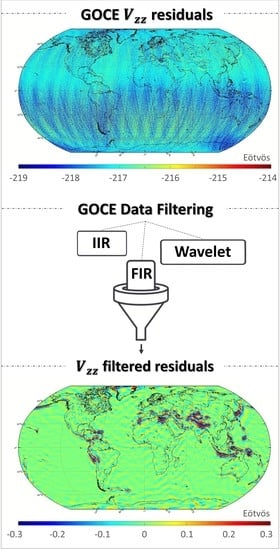
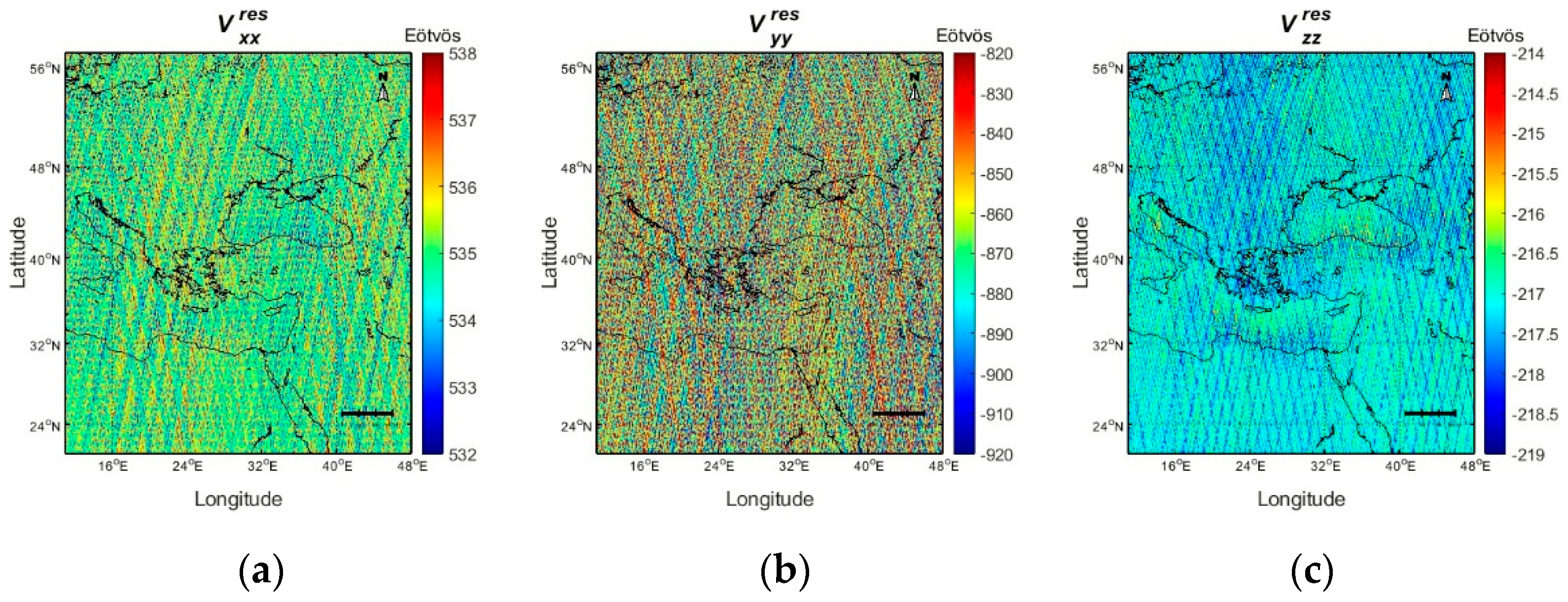
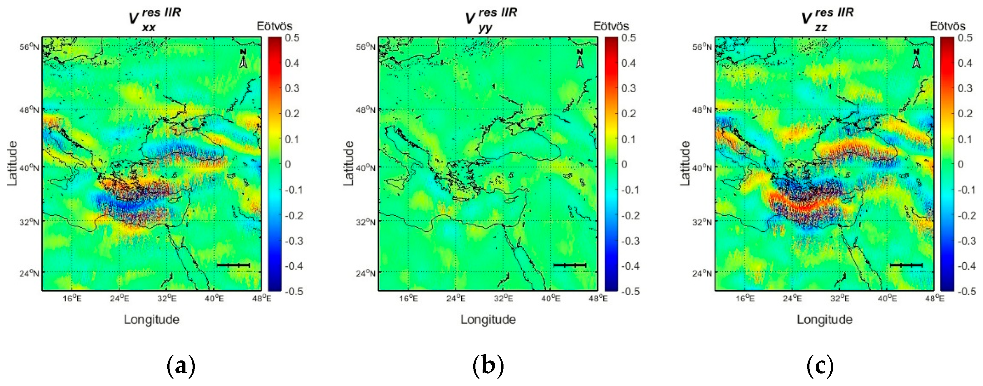
Figure 1.
The gravity gradient residuals (Eötvös) in the Gradiometer Reference Frame for (a) , (b) and (c) .
Figure 1.
The gravity gradient residuals (Eötvös) in the Gradiometer Reference Frame for (a) , (b) and (c) .
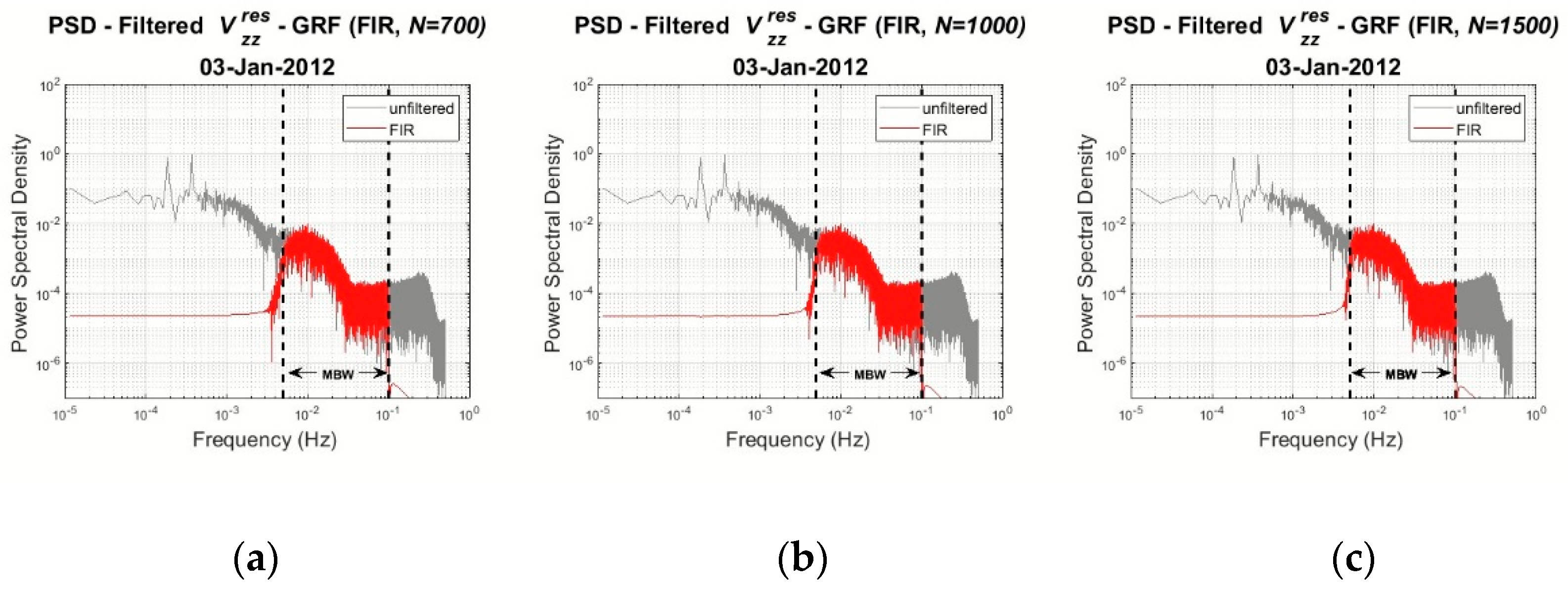
Figure 2.
PSDs of the filtered (red) and unfiltered (grey) residuals for (a) N = 700, (b) N = 1000 and, (c) N = 1500 filter order.
Figure 2.
PSDs of the filtered (red) and unfiltered (grey) residuals for (a) N = 700, (b) N = 1000 and, (c) N = 1500 filter order.
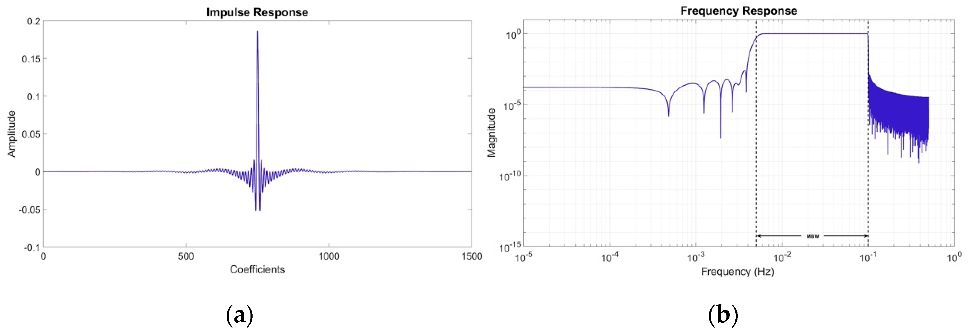
Figure 3.
(a) Impulse Response and (b) Frequency Response of a 1500th order FIR filter.
Figure 3.
(a) Impulse Response and (b) Frequency Response of a 1500th order FIR filter.
Figure 4.
FIR filter design procedure.
Figure 4.
FIR filter design procedure.
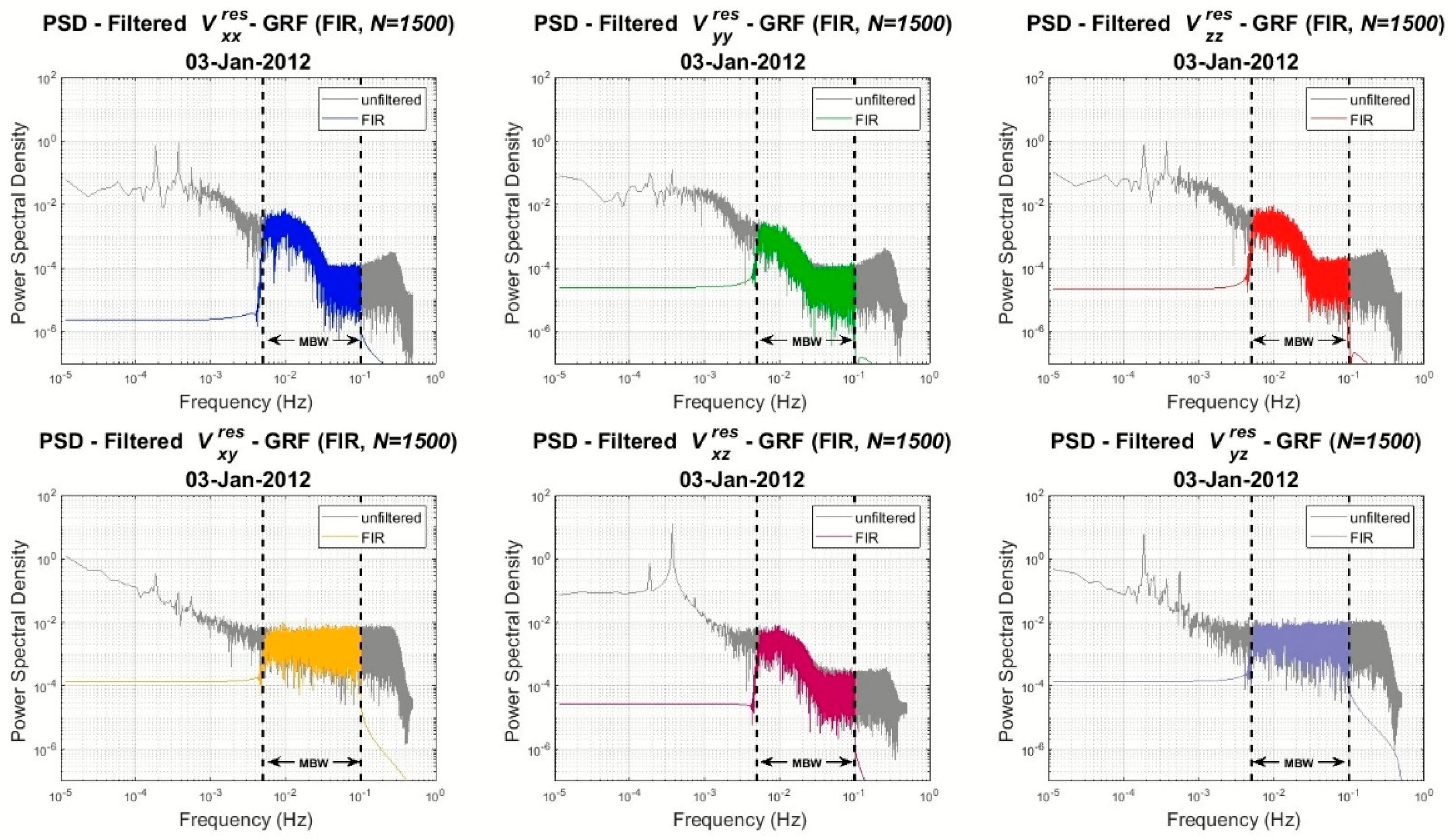
Figure 5.
PSDs of the filtered (colored ones) and unfiltered (grey) gravity gradient residuals for , , , , , .
Figure 5.
PSDs of the filtered (colored ones) and unfiltered (grey) gravity gradient residuals for , , , , , .
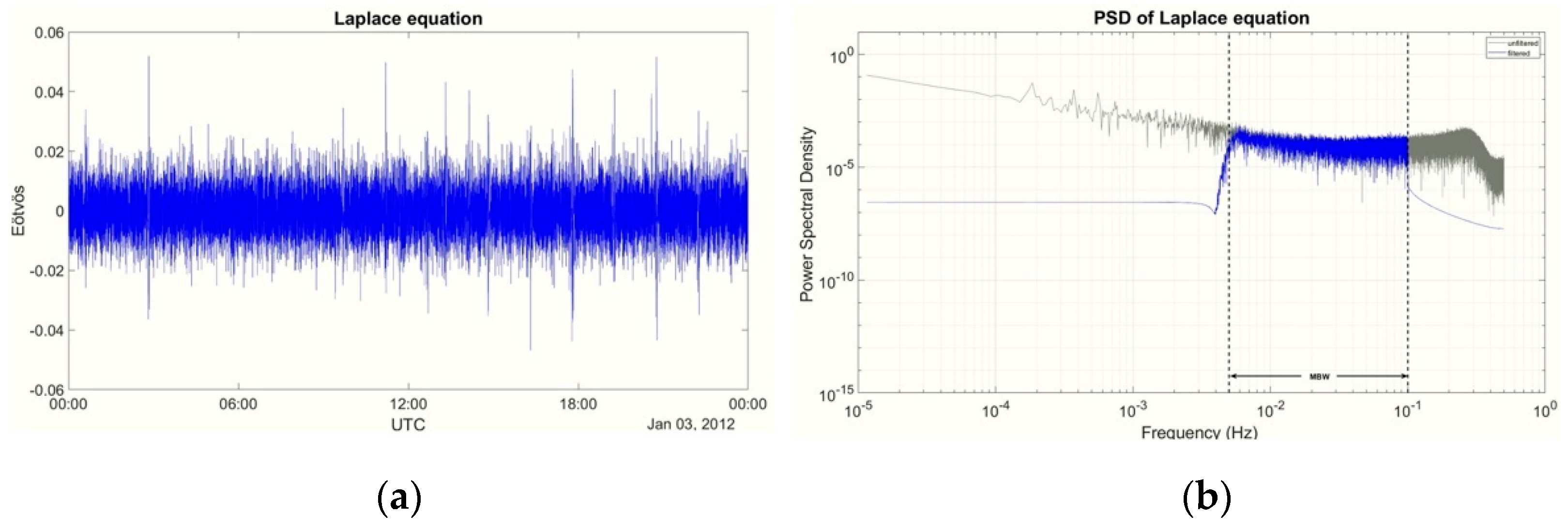
Figure 6.
Trace of the residual FIR filtered SGG tensor in (a) time domain and (b) frequency domain.
Figure 6.
Trace of the residual FIR filtered SGG tensor in (a) time domain and (b) frequency domain.
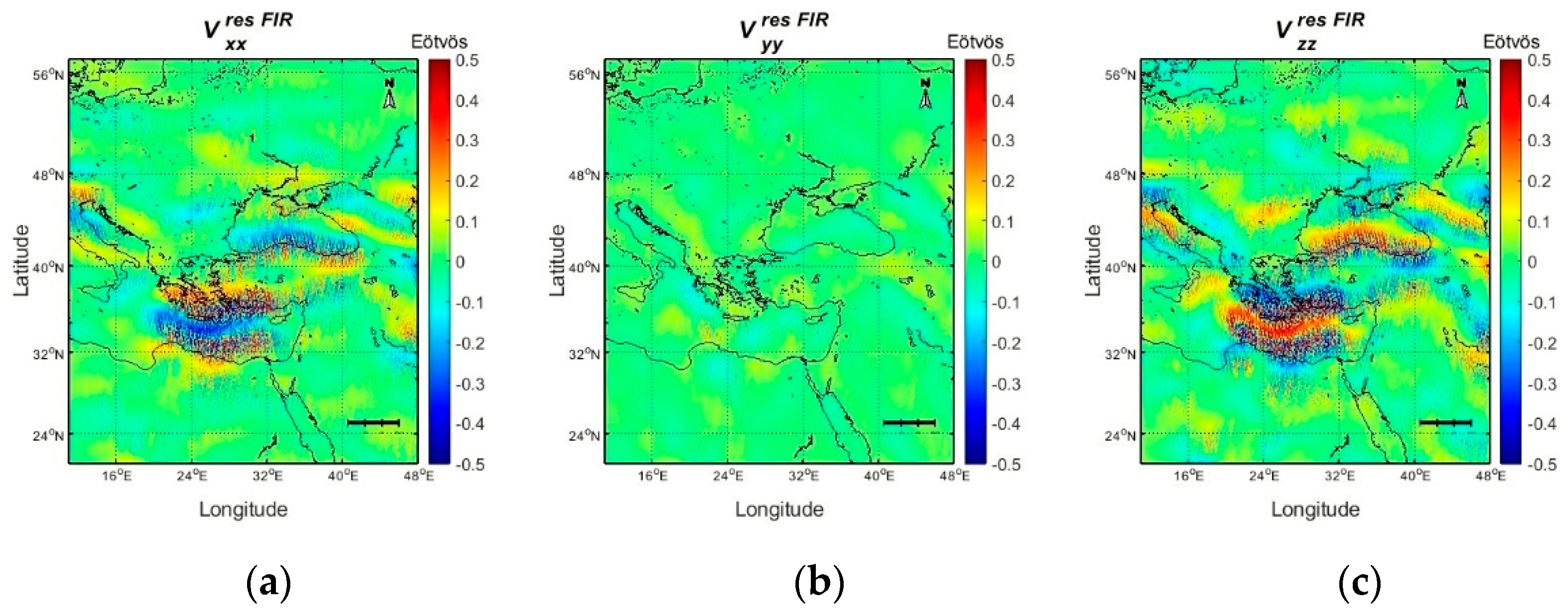
Figure 7.
FIR filtered residuals for components (a) , (b) and (c) .
Figure 7.
FIR filtered residuals for components (a) , (b) and (c) .
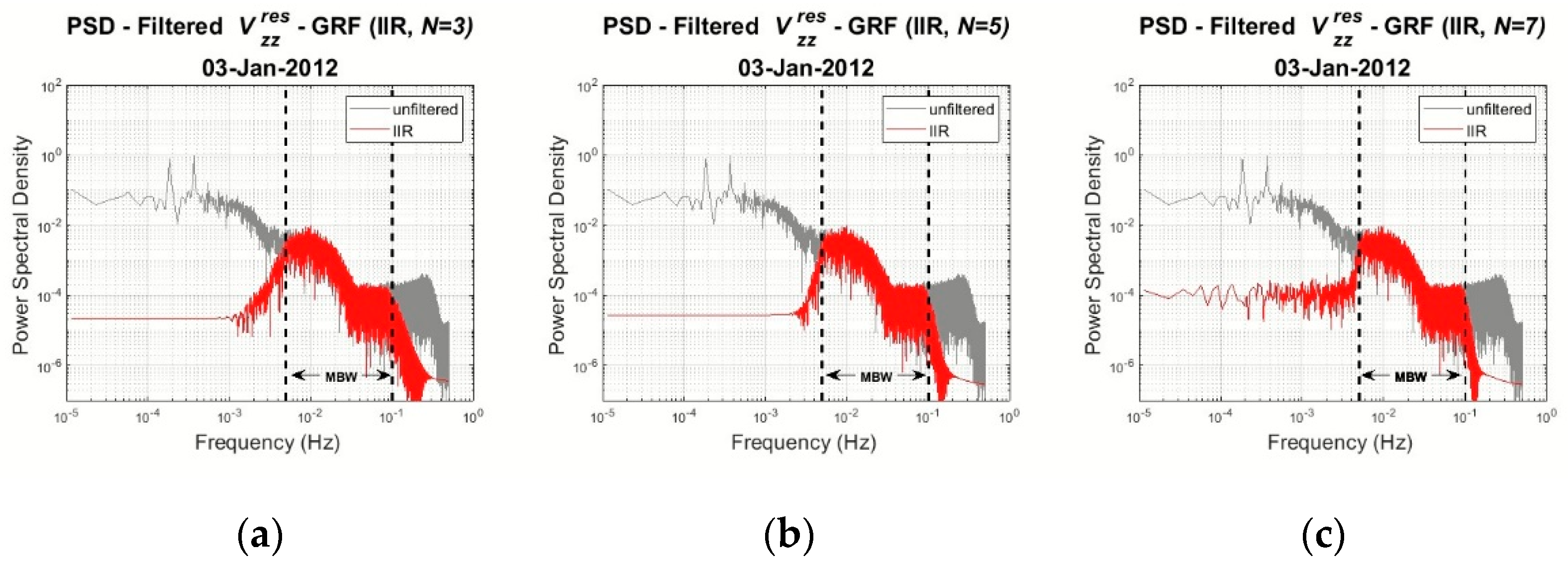
Figure 8.
PSDs of the filtered (red) and unfiltered (grey) for (a) N = 3, (b) N = 5 and, (c) N = 7 filter order.
Figure 8.
PSDs of the filtered (red) and unfiltered (grey) for (a) N = 3, (b) N = 5 and, (c) N = 7 filter order.
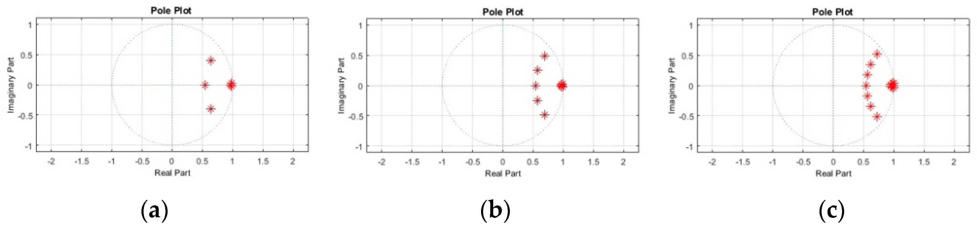
Figure 9.
Pole configuration of for bandpass filter order (a) N = 3, (b) N = 5 and, (c) N = 7.
Figure 9.
Pole configuration of for bandpass filter order (a) N = 3, (b) N = 5 and, (c) N = 7.
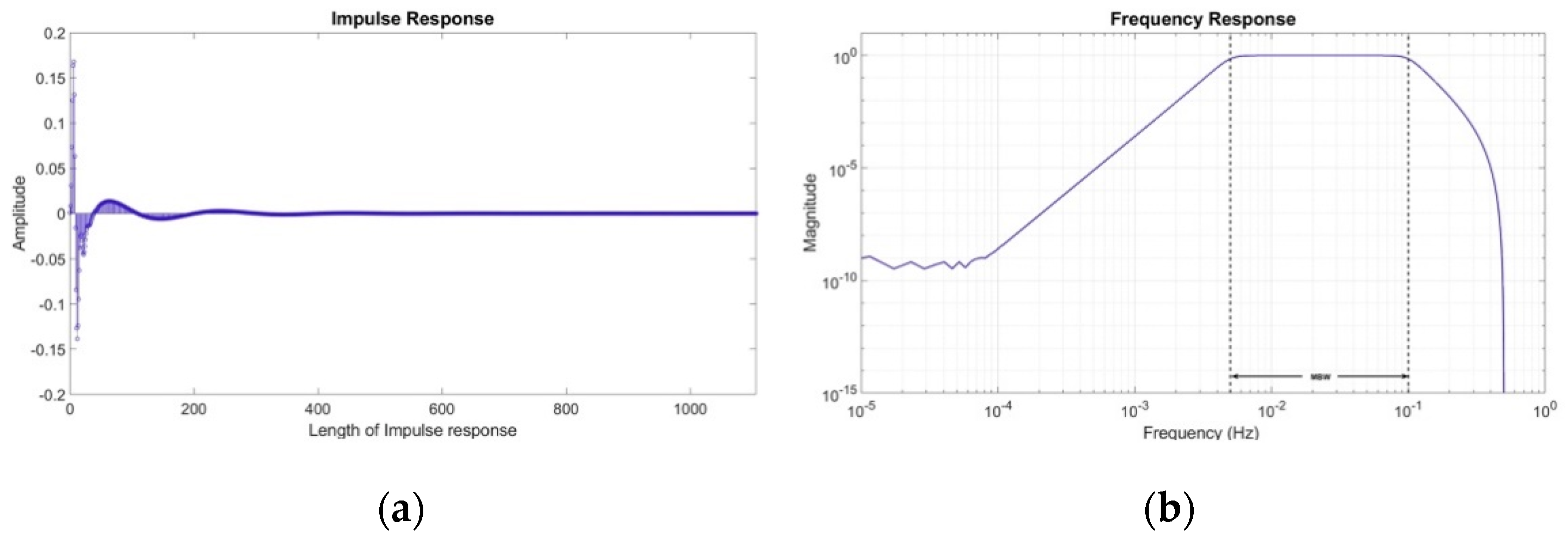
Figure 10.
(a) Impulse response and (b) frequency response of = 5 IIR Butterworth filter.
Figure 10.
(a) Impulse response and (b) frequency response of = 5 IIR Butterworth filter.
Figure 11.
IIR filter design procedure.
Figure 11.
IIR filter design procedure.
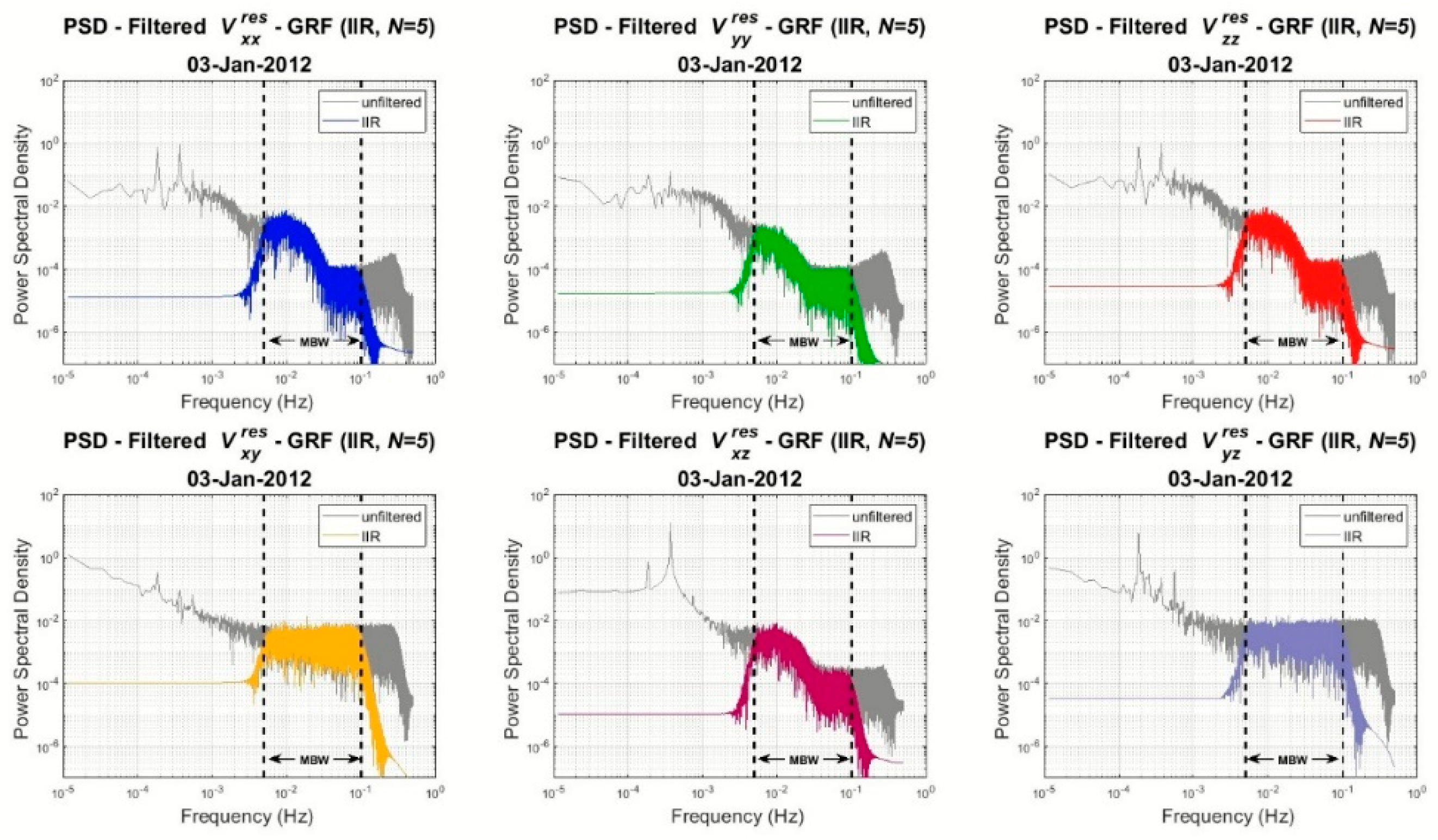
Figure 12.
PSDs of the filtered (colored ones) and unfiltered (grey) gravity gradient residuals for , , , , , .
Figure 12.
PSDs of the filtered (colored ones) and unfiltered (grey) gravity gradient residuals for , , , , , .
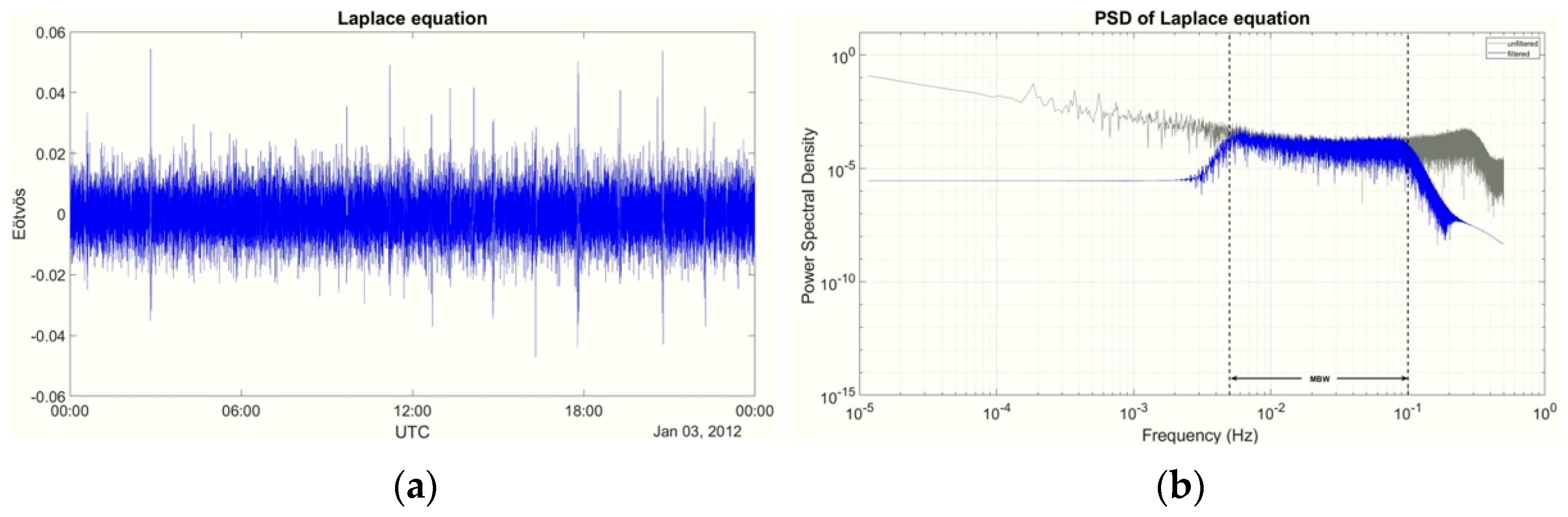
Figure 13.
Trace of the residual IIR filtered SGG tensor in (a) time domain and (b) frequency domain.
Figure 13.
Trace of the residual IIR filtered SGG tensor in (a) time domain and (b) frequency domain.
Figure 14.
IIR filtered residuals for components (a) , (b) and (c) .
Figure 14.
IIR filtered residuals for components (a) , (b) and (c) .
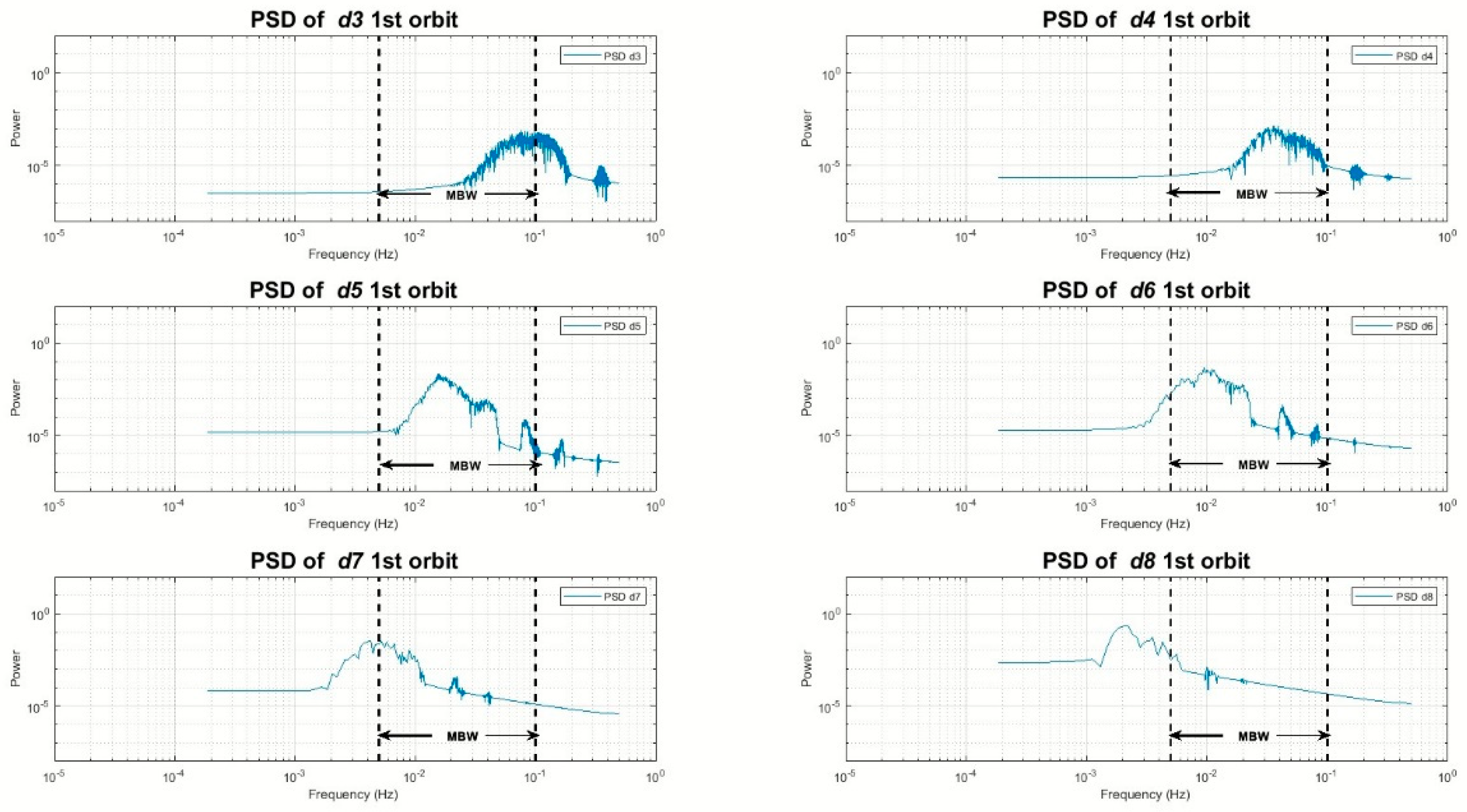
Figure 15.
PSDs of detail coefficients of levels 3, 4, 5, 6, 7 and 8 (d3, d4, d5, d6, d7, and d8) for one orbit of the Vzz component.
Figure 15.
PSDs of detail coefficients of levels 3, 4, 5, 6, 7 and 8 (d3, d4, d5, d6, d7, and d8) for one orbit of the Vzz component.
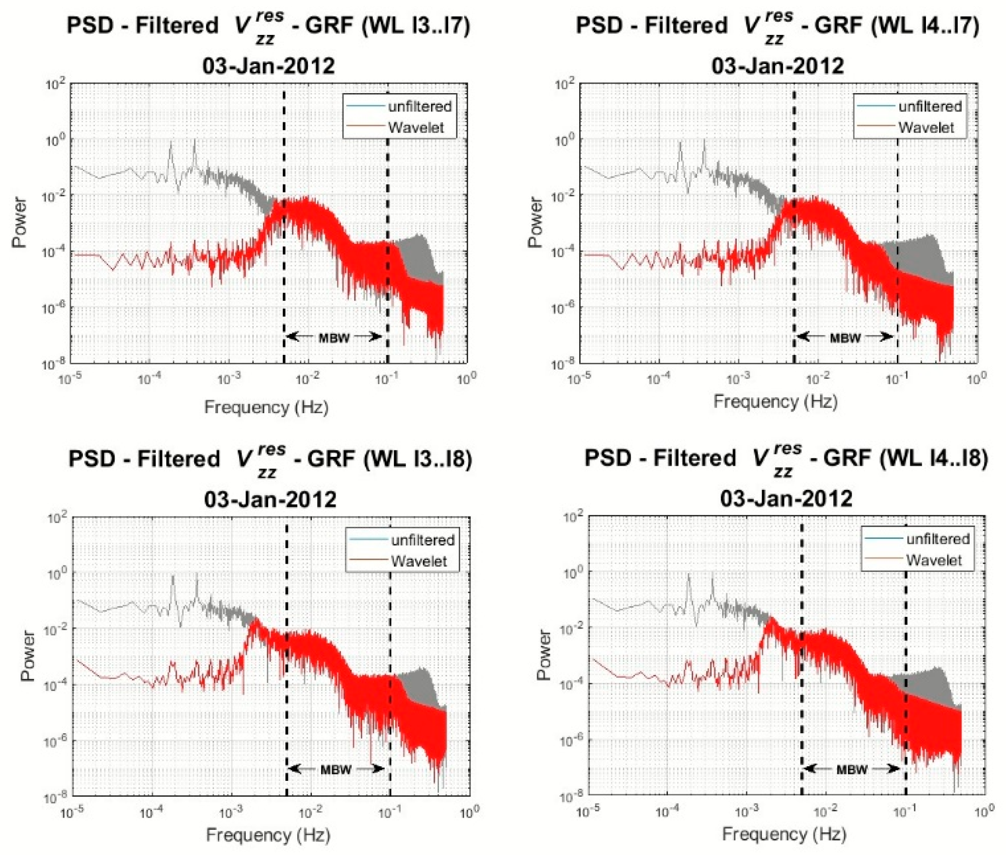
Figure 16.
PSDs of the filtered (red) and unfiltered (grey) gravity gradient for reconstruction l3..l7 (top left), reconstruction l4..l7 (top right), reconstruction l4..l8 (bottom left), and reconstruction l4..l8 (bottom right).
Figure 16.
PSDs of the filtered (red) and unfiltered (grey) gravity gradient for reconstruction l3..l7 (top left), reconstruction l4..l7 (top right), reconstruction l4..l8 (bottom left), and reconstruction l4..l8 (bottom right).
Figure 17.
Wavelet MRA design procedure.
Figure 17.
Wavelet MRA design procedure.
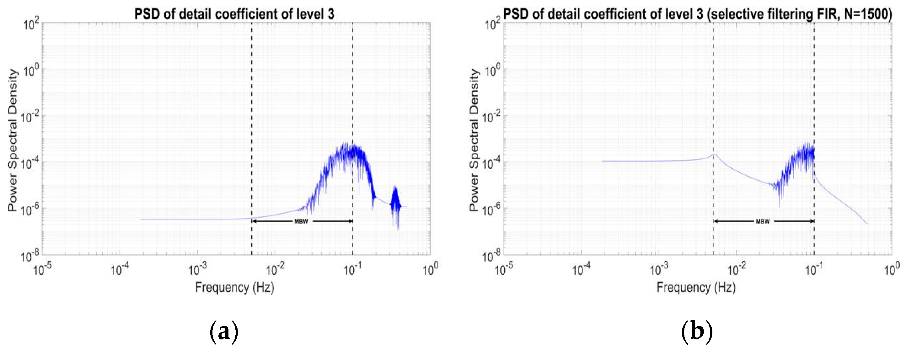
Figure 18.
PSDs of detail coefficients of level 3 (a) before and (b) after the selective filtering for one orbit of the component.
Figure 18.
PSDs of detail coefficients of level 3 (a) before and (b) after the selective filtering for one orbit of the component.
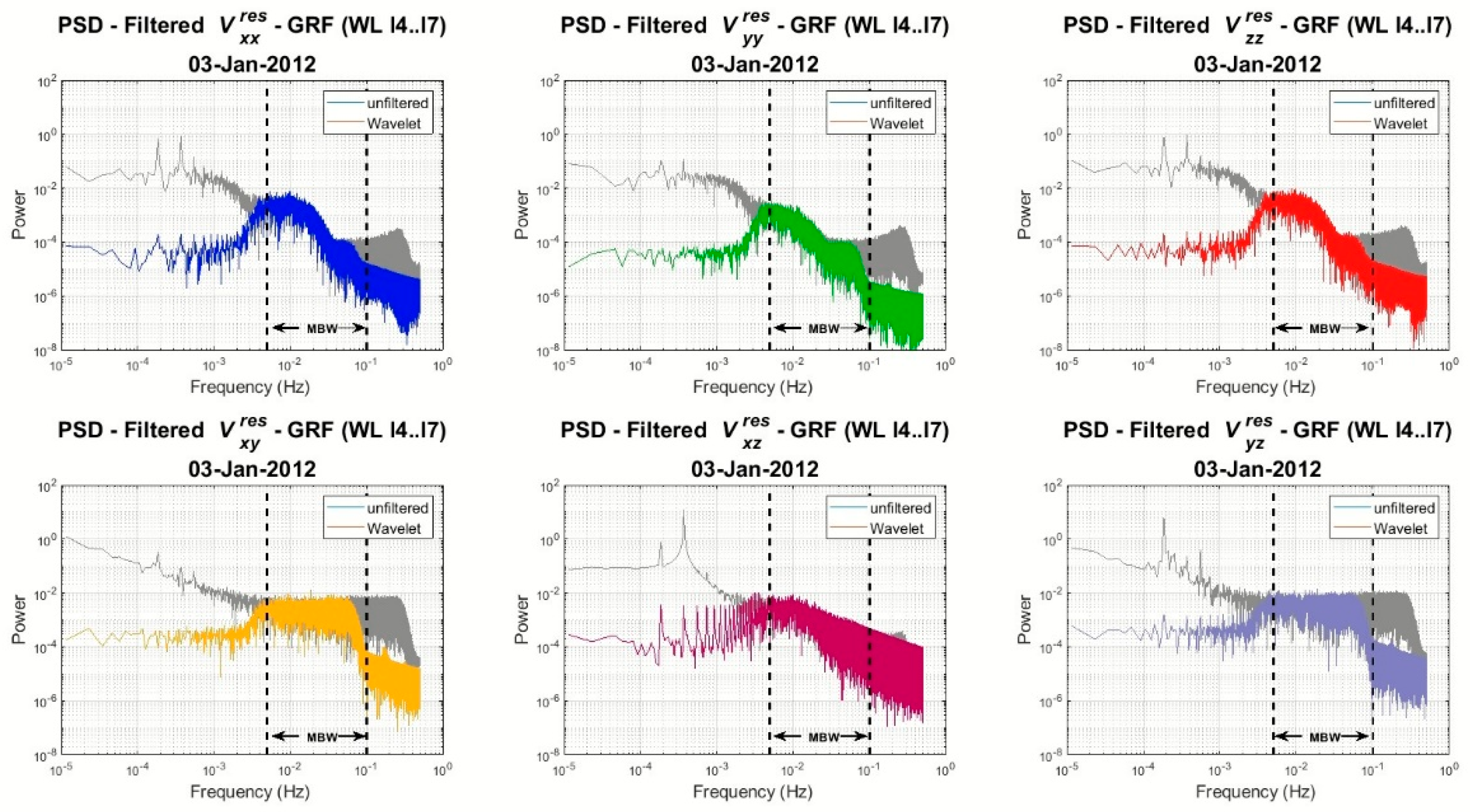
Figure 19.
PSDs of the filtered (colored ones) and unfiltered (grey) gravity gradient residuals after reconstruction l4..l7 for , , , , , .
Figure 19.
PSDs of the filtered (colored ones) and unfiltered (grey) gravity gradient residuals after reconstruction l4..l7 for , , , , , .
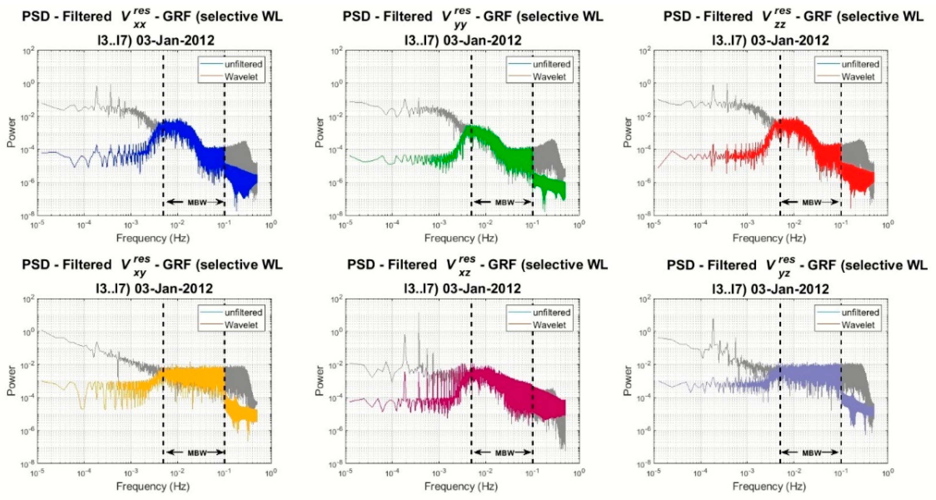
Figure 20.
PSDs of the filtered (colored ones) and unfiltered (grey) gravity gradient residuals after selective reconstruction l3filtl4..l7 for , , , , , .
Figure 20.
PSDs of the filtered (colored ones) and unfiltered (grey) gravity gradient residuals after selective reconstruction l3filtl4..l7 for , , , , , .
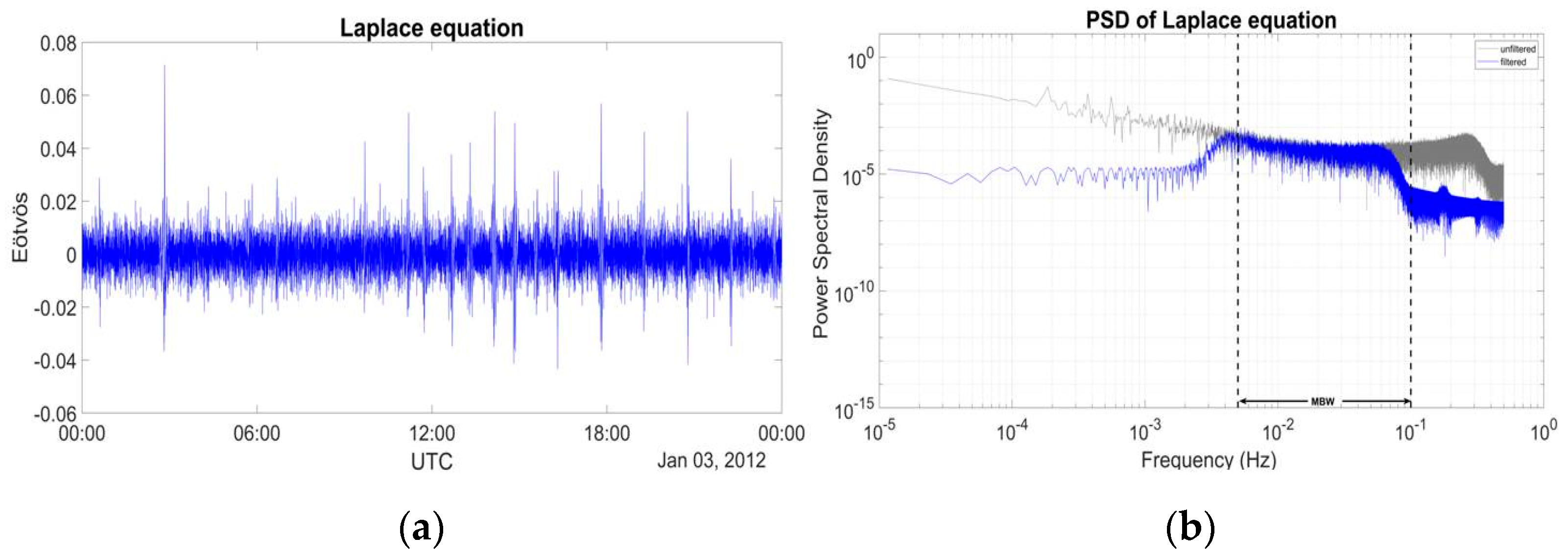
Figure 21.
Trace of the residual WL MRA filtered SGG tensor of the reconstruction l4..l7 for one day of data in (a) time domain and (b) frequency domain.
Figure 21.
Trace of the residual WL MRA filtered SGG tensor of the reconstruction l4..l7 for one day of data in (a) time domain and (b) frequency domain.
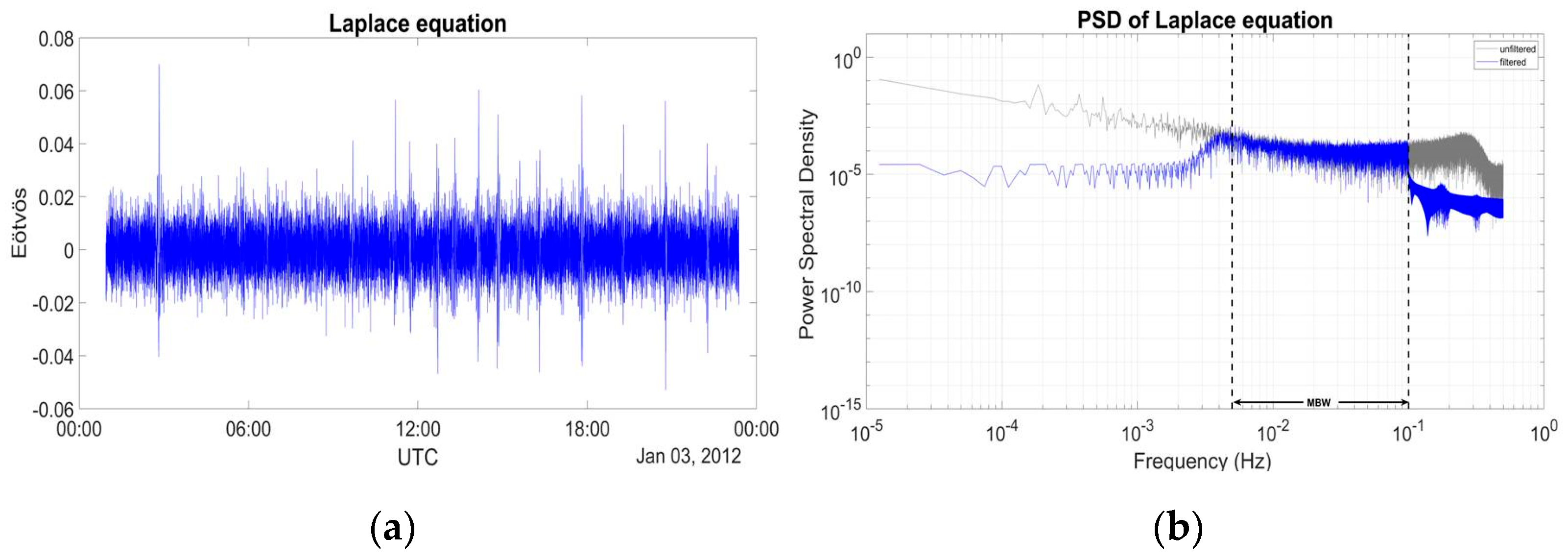
Figure 22.
Trace of the residual WL MRA filtered SGG tensor of the selective reconstruction l3filtl4..l7 for data of 15 full orbits in (a) time domain and (b) frequency domain.
Figure 22.
Trace of the residual WL MRA filtered SGG tensor of the selective reconstruction l3filtl4..l7 for data of 15 full orbits in (a) time domain and (b) frequency domain.
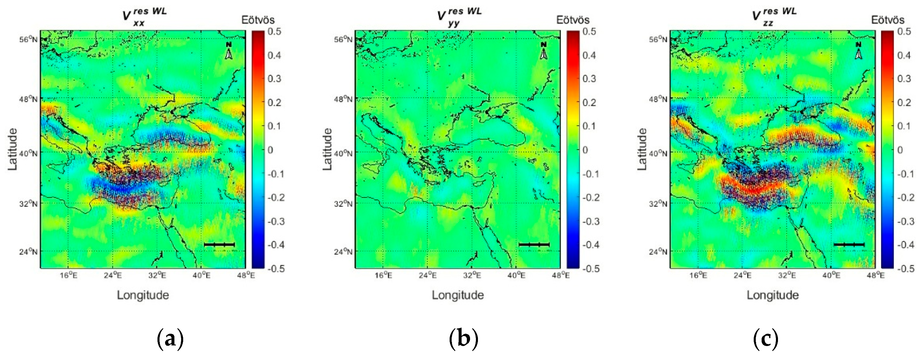
Figure 23.
The l4..l7 reconstruction based on one year of residual data (a) , (b) and (c) .
Figure 23.
The l4..l7 reconstruction based on one year of residual data (a) , (b) and (c) .
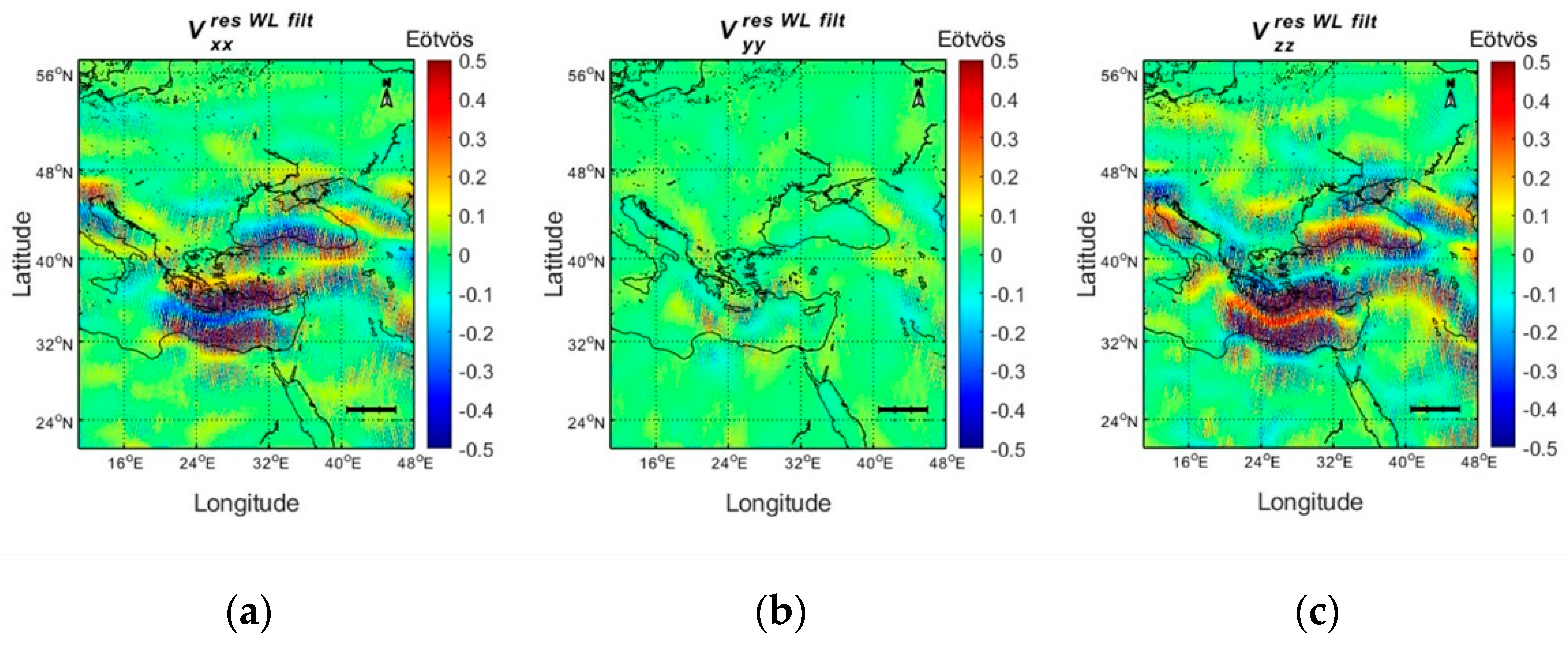
Figure 24.
The selective l3filtl4..l7 reconstruction based on one year of residual data (a) , (b) and (c) .
Figure 24.
The selective l3filtl4..l7 reconstruction based on one year of residual data (a) , (b) and (c) .
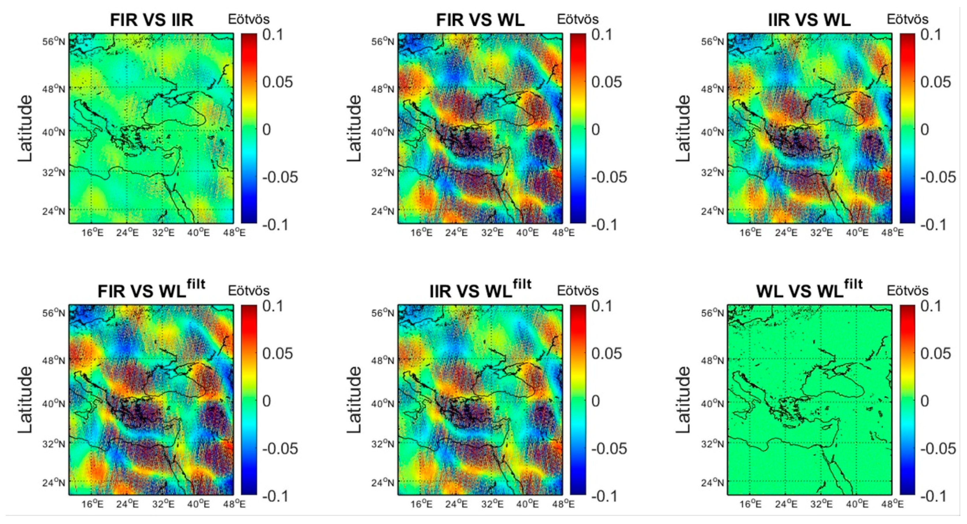
Figure 25.
differences between the FIR, IIR, WL and WLfilt residuals for FIR vs. IIR, FIR vs. WL, IIR vs. WL, FIR vs. WLfilt, IIR vs. WLfilt, and WL vs. WLfilt.
Figure 25.
differences between the FIR, IIR, WL and WLfilt residuals for FIR vs. IIR, FIR vs. WL, IIR vs. WL, FIR vs. WLfilt, IIR vs. WLfilt, and WL vs. WLfilt.
Table 1.
Statistics of the gravity gradient (GOCE, GGM, and residuals) in the Gradiometer Reference Frame. Units: [Eötvös].
Table 1.
Statistics of the gravity gradient (GOCE, GGM, and residuals) in the Gradiometer Reference Frame. Units: [Eötvös].
| Min | Max | Mean | Std | Rms |
|---|
| −845.3973 | −824.2611 | −833.0453 | 4.6350 | 833.0582 |
| −2288.4527 | −2185.6553 | −2230.5057 | 29.1599 | 2230.6963 |
| 2503.7758 | 2539.9047 | 2517.8606 | 7.7178 | 2517.8725 |
| −1379.2229 | −1360.4318 | −1367.6672 | 3.7218 | 1367.6723 |
| −1377.0201 | −1360.8739 | −1366.5978 | 3.5684 | 1366.6025 |
| 2721.4291 | 2756.2323 | 2734.2651 | 7.2474 | 2734.2747 |
| 312.5748 | 547.4686 | 535.0950 | 1.5400 | 535.0973 |
| −922.0031 | −806.0065 | −863.9518 | 33.2854 | 864.5927 |
| −219.4768 | −213.7558 | −217.1494 | 0.8303 | 217.1510 |
Table 2.
Laplace equation statistics for the unfiltered and filtered residuals. Units: [Eötvös].
Table 2.
Laplace equation statistics for the unfiltered and filtered residuals. Units: [Eötvös].
| Min | Max | Mean | Std | Rms |
|---|
| Unfiltered | −602.9003 | −602.2378 | −602.6038 | 0.1250 | 602.6038 |
| FIR | −0.0467 | 0.0518 | 0.0000 | 0.0077 | 0.0077 |
| IIR | −0.0470 | 0.0545 | 0.0000 | 0.0075 | 0.0075 |
| −0.0433 | 0.0715 | 0.0000 | 0.0072 | 0.0072 |
| −0.0529 | 0.0701 | 0.0000 | 0.0085 | 0.0085 |
Table 3.
Statistics of the FIR filtered residuals. Units: [Eötvös].
Table 3.
Statistics of the FIR filtered residuals. Units: [Eötvös].
| | Min | Max | Mean | Std | Rms |
|---|
| 312.5748 | 547.4686 | 535.0950 | 1.5400 | 535.0973 |
| −922.0031 | −806.0065 | −863.9518 | 33.2854 | 864.5927 |
| −219.4768 | −213.7558 | −217.1494 | 0.8303 | 217.1510 |
| −0.7859 | 0.7458 | 0.0007 | 0.1284 | 0.1284 |
| −0.2046 | 0.2545 | 0.0000 | 0.0381 | 0.0381 |
| −0.8844 | 0.8798 | −0.0007 | 0.1522 | 0.1522 |
Table 4.
Statistics of the IIR filtered residuals. Units: [Eötvös].
Table 4.
Statistics of the IIR filtered residuals. Units: [Eötvös].
| | Min | Max | Mean | Std | Rms |
|---|
| −0.7840 | 0.7531 | 0.0008 | 0.1280 | 0.1280 |
| −0.2027 | 0.2572 | 0.0000 | 0.0381 | 0.0381 |
| −0.8931 | 0.8804 | −0.0009 | 0.1518 | 0.1518 |
Table 5.
Resolution of the levels of decomposition.
Table 5.
Resolution of the levels of decomposition.
| Levels | Resolution (in km) | Levels | Resolution (in km) |
|---|
| Level 1 | 8 | 16 | Level 7 | 512 | 1024 |
| Level 2 | 16 | 32 | Level 8 | 1024 | 2048 |
| Level 3 | 32 | 64 | Level 9 | 2048 | 4096 |
| Level 4 | 64 | 128 | Level 10 | 4096 | 8192 |
| Level 5 | 128 | 256 | Level 11 | 8192 | 16,384 |
| Level 6 | 256 | 512 | Level 12 | 16,384 | 32,768 |
Table 6.
Statistics of the detail coefficient of level 3 before the selective filtering. Unit: [Eötvös].
Table 6.
Statistics of the detail coefficient of level 3 before the selective filtering. Unit: [Eötvös].
| | Min | Max | Mean | Std | Rms |
|---|
| −0.0123 | 0.0118 | 0.0000 | 0.0029 | 0.0029 |
| −0.0136 | 0.0118 | 0.0000 | 0.0027 | 0.0027 |
| −0.0149 | 0.0167 | 0.0000 | 0.0044 | 0.0044 |
Table 7.
Statistics of the detail coefficient of level 3 after the selective filtering. Unit: [Eötvös].
Table 7.
Statistics of the detail coefficient of level 3 after the selective filtering. Unit: [Eötvös].
| | Min | Max | Mean | Std | Rms |
|---|
| −0.0081 | 0.0080 | 0.0000 | 0.0021 | 0.0021 |
| −0.0090 | 0.0094 | 0.0000 | 0.0020 | 0.0020 |
| −0.0150 | 0.0120 | −0.0001 | 0.0033 | 0.0033 |
Table 8.
Statistics for the l4..l7 reconstruction for one year of data. Unit: [Eötvös].
Table 8.
Statistics for the l4..l7 reconstruction for one year of data. Unit: [Eötvös].
| | Min | Max | Mean | Std | Rms |
|---|
| −0.8524 | 0.7991 | 0.0005 | 0.1037 | 0.1037 |
| −0.2275 | 0.2737 | 0.0001 | 0.0378 | 0.0378 |
| −0.9641 | 0.9676 | −0.0005 | 0.1263 | 0.1263 |
Table 9.
Statistics for the selective l3filtl4..l7 reconstruction for one year of data. Unit: [Eötvös].
Table 9.
Statistics for the selective l3filtl4..l7 reconstruction for one year of data. Unit: [Eötvös].
| | Min | Max | Mean | Std | Rms |
|---|
| −0.8535 | 0.8021 | 0.0005 | 0.1237 | 0.1037 |
| −0.2273 | 0.2725 | 0.0001 | 0.0378 | 0.0378 |
| −0.9615 | 0.9698 | −0.0005 | 0.1263 | 0.1263 |
Table 10.
Statistics of differences between the FIR, IIR and WL MRA filtered residuals. Unit: [Eötvös].
Table 10.
Statistics of differences between the FIR, IIR and WL MRA filtered residuals. Unit: [Eötvös].
| | Min | Max | Mean | Std | Rms |
|---|
| −0.0407 | 0.0407 | 0.0002 | 0.0114 | 0.0114 |
| −0.2065 | 0.2156 | 0.0011 | 0.0486 | 0.0486 |
| −0.1695 | 0.1779 | 0.0009 | 0.0400 | 0.0400 |
| −0.2064 | 0.2131 | 0.0011 | 0.0485 | 0.0485 |
| −0.1691 | 0.1772 | 0.0009 | 0.0399 | 0.0399 |
| −0.0163 | 0.0160 | 0.0000 | 0.0033 | 0.0033 |


 ,
, 


