Article

UAV Remote Sensing for High-Throughput Phenotyping and for Yield Prediction of Miscanthus by Machine Learning Techniques

1
Department of Sustainable Crop Production, Università Cattolica del Sacro Cuore, 29122 Piacenza, Italy
2
Remote Sensing and Spatial Analysis Research Center (CRAST), Università Cattolica del Sacro Cuore, 29122 Piacenza, Italy
3
Institute of Biological, Environmental and Rural Sciences (IBERS), Aberystwyth University, Aberystwyth SY23 3EE, UK
4
Terravesta, Unit 4 Riverside Court, Skellingthorpe Road, Saxilby, Lincoln LN1 5AB, UK
5
Department of Biobased Resources in the Bioeconomy, Institute of Crop Science, University of Hohenheim, 70599 Stuttgart, Germany
6
Department of Plant Breeding, Wageningen University & Research, 6700 AJ Wageningen, The Netherlands
7
Institute for Electromagnetic Sensing of the Environment, National Research Council, 20133 Milan, Italy
8
Institut für Pflanzenbau und Pflanzenzüchtung I, Justus-Liebig-Universität Gießen, Heinrich-Buff-Ring 26, 35392 Gießen, Germany
*
Author to whom correspondence should be addressed.
Remote Sens. 2022, 14(12), 2927; https://doi.org/10.3390/rs14122927
Submission received: 7 June 2022 / Revised: 16 June 2022 / Accepted: 17 June 2022 / Published: 19 June 2022

Abstract

:
Miscanthus holds a great potential in the frame of the bioeconomy, and yield prediction can help improve Miscanthus’ logistic supply chain. Breeding programs in several countries are attempting to produce high-yielding Miscanthus hybrids better adapted to different climates and end-uses. Multispectral images acquired from unmanned aerial vehicles (UAVs) in Italy and in the UK in 2021 and 2022 were used to investigate the feasibility of high-throughput phenotyping (HTP) of novel Miscanthus hybrids for yield prediction and crop traits estimation. An intercalibration procedure was performed using simulated data from the PROSAIL model to link vegetation indices (VIs) derived from two different multispectral sensors. The random forest algorithm estimated with good accuracy yield traits (light interception, plant height, green leaf biomass, and standing biomass) using 15 VIs time series, and predicted yield using peak descriptors derived from these VIs time series with root mean square error of 2.3 Mg DM ha−1. The study demonstrates the potential of UAVs’ multispectral images in HTP applications and in yield prediction, providing important information needed to increase sustainable biomass production.

Graphical Abstract

1. Introduction

Miscanthus is a high yielding perennial biomass crop. Yield is one of the most important traits of Miscanthus [1] and has been the primary focus of the research portfolio on Miscanthus in the last ten years [2,3,4]. Independent and collaborative efforts to breed high-yielding Miscanthus hybrids to produce sustainable biomass for the growing bio-based European market are ongoing in several countries [5,6,7]. In the EU-BBI demo-project GRACE, novel and highly upscalable seed-based Miscanthus hybrids are evaluated [5,7,8,9,10] in seven European countries. Most yield prediction to date has relied on crop growth models driven by climate and soil data with crop specific parameters [11,12,13]. For example, MISCANFOR is a crop growth model specifically developed to predict Miscanthus × giganteus yields in a wide range of environments [14]. It has been widely used and validated at the European [6] and national level [15] for Miscanthus and other perennial biomass crops [16], but new parameterization data to predict yield production of the novel Miscanthus hybrids [5] is required [14].
Yield trait screening and prediction using remote sensing with unmanned aerial vehicles (UAVs) can help both in breeding activities and in obtaining spatial and temporal information for optimizing Miscanthus biomass supply chain logistics, from field to facilities creating bioproducts or biopower [17,18]. Impollonia et al. [19] recently demonstrated the feasibility of moisture content estimation in Miscanthus hybrids using vegetation indices (VIs) derived from UAV-based remote sensing. Remote sensing approaches can also be used to (i) estimate yield-related traits for high-throughput phenotyping (HTP) [20,21,22], (ii) to calibrate crop growth models [23,24], and (iii) to predict the yield of many crops for commercial purposes [25]. To date, few studies have focused on the estimation and prediction of perennial biomass crops traits using remote sensing technologies from satellite or UAV [26,27,28], and only two on Miscanthus [18,19]. Crop traits such as the plant height [29], the fraction of absorbed photosynthetically active radiation (fAPAR) [30], and the aboveground biomass [31] can be estimated from the VIs in combination with machine learning (ML) algorithms. One of the most used ML algorithms in remote sensing analyses for crop traits estimation is random forest (RF) [32,33,34,35]. RF proved to be robust to outliers and noise, does not suffer from overfitting, and can manage a high training size [36]. The use of ML algorithms demonstrates great potential in crop yield prediction [37,38,39,40]. In particular, the use of a VIs’ time series helped to derive descriptors of land surface phenology (LSP, i.e., the spatial and temporal development of the vegetated land surface) [41,42,43,44,45] such as the start of season (SOS), the peak of growing season, the stay-green duration (onset of senescence), the end of the season (EOS), and growing season length [46]. Among the available descriptors of LSP, the peak of a VI is one of the most important descriptors for crop yield prediction, such as the peak of NDVI [47] and EVI2 [17] for grain yield and the peak of GNDVI for biomass yields of perennial grass [26]. Yield prediction is, in many studies, theoretical, as it requires to fit the whole seasonal curve for deriving the peak of the time series of VIs. This renders impossible the yield prediction before having obtained the data of the whole seasonal time series. Being able to perform yield prediction months before harvest with a partial time series should permit optimization of Miscanthus biomass supply chain logistics for practical applications.
In addition, the VIs’ values used for estimation and prediction of crop traits are influenced by many factors, such as sensor characteristics, atmospheric conditions during acquisition, viewing angle, field of view, and sun elevation [48]. In the context of crop phenotyping, where the field trials are often carried out in multi-locations and with different UAV sensors, these factors could have a relevant effect on the compatibility of VIs. Among different sensors characteristics, the full width at half maximum (FWHM) is the main factor that influences the comparability of VIs’ values among different sensors [49]. Indeed, due to the different spectral characteristics of the UAV multispectral sensors available on the market, differences among VIs derived from multiple UAV sensors for the same target can be found [48]. For this reason, there is a need to increase the interoperability of the sensors using equations that are able to overcome these differences through advanced linking procedures between the VIs of sensors [50,51]. The multi-sensor interoperability is an important topic in remote sensing science [52,53,54] when multi-location monitoring is conducted. Overcoming this problematic can be realised by intercalibrating the VIs obtained by different sensors and evaluating the correlation through linear regressions [55,56,57]. This intercalibration can be realised in two main ways: a direct approach where VIs are measured by sensors [58] and an indirect approach where VIs data are simulated by radiative transfer models [59]. A major limitation of the direct regression approach is that it is not transferable because it is site-specific [50]. On the contrary, the indirect approach permits retrieval of VIs’ data from radiative transfer models, such as the PROSAIL model [60,61]. The PROSAIL model is commonly used for the retrieval of biochemical and biophysical crop traits from remotely sensed images for vegetation studies in agricultural applications [62]. PROSAIL has also been used to assess the performances of different satellite sensors for multiple VIs [63], but a similar application is currently lacking in UAV science. Hence, the use of such an approach for VIs’ intercalibration in UAV science might allow for overcoming the problematic of multi-sensor interoperability across different sites.
In summary, the overall objectives of this study, based on UAV remote sensing, were: (i) to estimate crop traits (light interception, plant height, green leaf biomass, and standing biomass) for supporting breeding programs and for providing modelling parameters for Miscanthus, (ii) to predict yield to obtain spatial and temporal information for improving the logistics biomass supply chain of Miscanthus, and (iii) to explore the potential impact of the timeliness on the yield prediction, by evaluating the performance of the yield prediction model using the peak derived from a partial time series of VIs. To achieve these overarching objectives, UAV multispectral images and ground phenotypic data were collected at two locations within the same multi-environment trial: one in Italy and one in the UK. These data were analysed using: (i) the PROSAIL model to simulate crop spectral signatures in order to intercalibrate VIs of two different common multispectral sensors, (ii) the random forest (RF) algorithm to estimate crop traits using the VIs time series and to predict yield using the peak descriptor derived from the VIs time series, for the reliability it achieved in previous studies [17,26,47], and (iii) the generalized additive model (GAM) to derive the peak from a complete and partial time series of VIs.

2. Materials and Methods

2.1. Experimental Design

The field trials were conducted in two locations (Figure 1): PAC 1, located in San Bonico in the Italian province of Piacenza (NW Italy) (45°00′11.70″ N, 9°42′35.39″ E), and TWS 1, located in Trawscoed near Aberystwyth in Wales (UK) (52°24′59.8″ N, 4°04′02.6″ W). These sites are two of the seven plot scale (PS) trials conducted within the EU-BBI GRACE demo-project. In PAC 1, the climate is temperate with a mean annual precipitation of 792 mm, while the climate in TWS 1 is oceanic with a mean annual precipitation of 984 mm. The trials were established in April 2018 with 14 Miscanthus hybrids with n = 4 replicates for a total of n = 56 plots. The trials were planted with eight novel intraspecific M. sinensis × M. sinensis hybrids (M. sin × M. sin), five novel interspecific hybrids M. sinensis × M. sacchariflorus (M. sin × M. sac), and M. × giganteus as the control genotype (for more details see Impollonia et al. [19]).

2.2. Phenotypic and Yield Measurements

Phenotypic measurements were taken from the emergence of the crop in spring 2020 until the winter harvest in the early months of 2021. This season will thereafter be referred to as the 2020 growing season. These phenotypic measurements were carried out in the two locations and on four out of the fourteen hybrids in the trial: GRC 3 (M. sin × M. sin), GRC 14 (seeded) and GRC 15 (clonal) (M. sin × M. sac), and GRC 9 (standard clonal M. × giganteus). The measurements of this study were carried out during the third growing season. Five contiguous plants along a central row in each plot were used for monitoring during the growing season. The following list of crop traits were measured during the growing season: plant height (cm) and light interception (%) were measured weekly, and green leaf biomass (Mg DM ha−1) and standing biomass (Mg DM ha−1) were measured fortnightly; 172 and 145 data were collected for light interception, 240 and 204 for plant height, 232 and 316 for green leaf biomass, and 268 and 328 for standing biomass in PAC 1 and TWS 1, respectively. Plant height was measured from the soil to the height of the last ligule of the tallest stem using a graduated pole until the crop reached complete flowering or started to senesce in November. Light interception was measured with a lab-constructed 1 m “line ceptometer” with 10 photodiodes at 10 cm spacings, generating an electric current that is converted with simple circuitry to a voltage linearly proportional to the light intensity. Light intensity was measured above the canopy and at the base of each of the five selected plants. Light interception measurements were carried out from emergence until full canopy closure (around 95% of light is intercepted by the crop canopy) on a weekly basis and later at a lower frequency. Standing aboveground biomass was estimated on a monthly basis, starting after emergence in 2020 until harvest in winter 2021. Ten randomly sampled shoots per plot each fortnight (aka “serial cuts”) were related to the final quadrat yields at spring harvest and used to back calculate the seasonal dynamics of above ground biomass (Mg DM ha−1) from spring emergence until final harvest in the following spring. Each 10 shoot serial cuts were separated into green leaf, brown leaf, and stem fractions. The fresh weight measured in the field and the dry weight measured after oven drying to a constant weight at 80 °C were used to calculate the mass and moisture contents of each fraction and were scaled to Mg DM ha−1. The crop’s phenological stages were estimated using thermal time accumulation, following the method proposed on M. × giganteus by Tejera et al. [64]. Two main phenological stages were estimated: vegetative growth and senescence. The GDD accumulation started at plant emergence, and the accumulation of 1500 GDD was used as the threshold marking the difference between the vegetative growth and senescence. The final harvested yield was measured for all 14 hybrids, using a quadrat area of 6.6 m2 (10 plants per plot planted at 1.5 plants m−2 (M. × giganteus and M. sin × M. sac) or 20 plants per plots at 3 plants m−2 (M. sin × M. sin)) and a cutting height of 10 cm. In each plot, the fresh weight of all plants in the quadrat was recorded, and a subsample of approximately five stems per plot was used to determine the moisture content and calculate the yield in Mg DM ha−1. Plants were harvested on 02 February 2021 (Days of year (DOY): 33) at PAC 1 and on 08 March 2021 (DOY: 67) at TWS 1.

2.3. UAV Multispectral Data and Vegetation Indices

Unmanned aerial vehicle (UAV) multispectral data acquisition flights were performed approximately fortnightly from 24 April 2020–1 February 2021 at the PAC 1 (25 flights) site and from 9 June 2020–25 February 2021 at the TWS 1 (17 flights) site (Table S1). Table 1 details the specifications of the UAVs and the multispectral cameras used at the two sites. All the flights were performed between 11 a.m. and 3 p.m., with the flight altitude above ground level (AGL) fixed at 50 m and 40 m at PAC 1 and TWS 1, respectively. The forward and lateral overlap was set at 80% and 75% of the images, respectively. Light sensors mounted on top of the UAVs were used for the radiometric calibration of the images. In addition, in PAC 1, images of the reflectance panel provided by MicaSense were also taken for calibrating images, to reduce the effects of the day’s changing lighting conditions during the flight [65]. The radiometric calibration and orthomosaic generation were done using the Pix4D mapper (Pix4D, S.A., Lausanne, Switzerland). The 15 vegetation indices (VIs) were calculated as illustrated in Table 2, using the orthomosaic. The mean of the VIs was extracted for each plot using the polygons of the experimental designs that were drafted in AutoCAD (Autodesk; San Rafael, CA, USA) and georeferenced with QGIS software (QGIS Development Team, 2021).

2.4. Using the PROSAIL Model to Intercalibrate VIs from Different Multispectral Sensors

The PROSAIL model was used to simulate crop spectral signatures to intercalibrate the VIs (Table 2), calculated from the two different multispectral sensors used in this study (Table 1). PROSAIL can simulate the canopy reflectance, between 400 and 2500 nm, by combining the PROSPECT and SAIL models. The PROSPECT model simulates the optical properties of the leaves using four input parameters: leaf structure parameter (N), leaf chlorophyll content (LCC), relative leaf equivalent water thickness (Cwr), and leaf dry matter content (Cm). The SAIL model simulates the bidirectional reflectance of a canopy using six input parameters: leaf area index (LAI), leaf inclination distribution (LIDF), hotspot parameter (hot), solar zenith angle (tts), observer zenith angle (tto), and relative azimuth angle (psi). The canopy and leaf parameters for Miscanthus were retrieved from available data in the literature [78,79]. The hsdar R package [80] was used to simulate the canopy reflectance of the PROSAIL model [60,61] using the function PROSAIL which uses the FORTRAN code of the PROSAIL model (Version 5B). The look-up table (LUT) generated included 430,080 parameter combinations, following the min-max ranges of input parameters summarized in Table 3.
The present work considers all potential parameter combinations for LUT generation because the novel Miscanthus hybrids evaluated have not previously been studied in the literature, and because the crop monitoring was performed on the whole growing season (vegetative growth and senescence). The spectral reflectance simulated were resampled based on the UAV sensor characteristics (Table 1) and the 15 VIs used in this study were calculated. For each VI, regression analysis was conducted to intercalibrate the VI values calculated from the two multispectral sensors. Linear regressions were performed using the VIs and not the spectral bands, in order to (i) evaluate the different sensitivity of the VIs to sensor characteristics and (ii) identify which VIs need an intercalibration procedure between sensors. The final database of VIs was built by scaling the SlantRange sensor VIs data toward the MicaSense sensor.

2.5. Time Series of VIs and Peak Derivation

The 15 Vis, calculated from UAV multispectral images of the two sites and intercalibrated using the linear models derived by the PROSAIL simulation, were smoothed using a generalized additive model (GAM) to generate daily VIs time series. The GAM is a non-parametric regression model which allows non-linear fitting of the variables. GAM models were fitted in the R package “mgcv” [81]. GAM fitting of VIs allows for removal of the outliers and regularizes the time series [19,82,83]. The time series of VIs for each plot were fitted against the modified days of the year (DOYM). The DOYM was used to overcome the problem of having non-sequential DOY throughout the growing season, as this last season overlaps two different years. DOYM were calculated as conventional DOY for the first year of the growing season (2020) and as DOY + 365 starting from the 1st of January for the year 2021.
The daily time series of the VIs were used to estimate the crop traits by linking the traits values measured in the field with the VIs’ values of the time series. To predict yield, the peak descriptor was chosen among several land surface phenology (LSP) descriptors, due to the reliability it achieved in previous studies [17,26,47]. The peak descriptor is defined as the maximum value and was derived from the GAM fitting of each VI time series. Two types of VIs time series were evaluated to derive the peak descriptor value: the complete and partial times series. The complete Vis time series were obtained by fitting the GAM models to the VIs’ data acquired throughout the entire growing season. The partial time series were obtained in two steps. Firstly, by fitting the GAM models to the VIs’ values, obtained from a reduced set of initial UAV flights over the crop. The first seven flights (175 DOY in PAC 1 and 266 DOY in TWS 1) were selected to form this reduced set of initial UAV flights, based on the physiology and phenology of Miscanthus, to cover most of the vegetative phase, the seventh flight being close to the peak of biomass accumulation. Secondly, the VIs’ data obtained from the following UAV flights were added one by one to the data fitted in the first step, up to the end of the season. The peak derived from the complete time series of VIs were used for the yield prediction modelling, and those from the partial time series of VIs were used to analyse the variation of peak values and the model performance in order to assess feasibility of “early season” yield prediction during Miscanthus crop growth.
The random forest (RF) algorithm was used to estimate the crop traits (Section 2.2) and to predict the yield of Miscanthus hybrids. The RF models were created using the caret R package [84]. Three steps in RF modelling were adopted. Firstly, RF models were created for (i) traits estimation, using the 15 VIs of the 4 Miscanthus hybrids (see Section 2.2) and phenological stages (encoded as 0 and 1 for the stages of vegetative growth and senescence, respectively) and (ii) yield prediction, using the peak values derived from the complete time series of the 15 investigated VIs of the 14 Miscanthus hybrids. Secondly, the importance of variables for each tested RF model was calculated by the dropout loss of the root mean square error (RMSE), and the variables with a median of RMSE loss greater than 0 were selected. Thirdly, the RF models used to estimate the variable of interest (i.e., crop traits or yield) were created using only the selected variables. The optimal size of the variable subset (“mtry”) for each model was obtained by a grid-searching method, using repeated k-fold cross-validation (ten-fold cross validation repeated five times). The training dataset was created using a stratified random sampling method [31]: data from both locations and genotypes were split into 2/3 of the dataset for training and 1/3 for testing, based on data distribution. The variable importance was calculated by the dropout loss of the RMSE (i.e., the increase of prediction in the RMSE [85]) using the DALEX package [86]. To demonstrate the uncertainty of importance estimation, the variable importance was calculated for 10 permutations [85]. The RF models’ performances were evaluated through the coefficient of determination (R2), the root mean square error, and the normalized root mean square error (NRMSE) [87]. The NRMSE was calculated by normalizing the RMSE using the mean of the measured values [19]. The RMSE and NRMSE metrics were also used to compare the performance of the yield prediction model using test datasets, with the peak derived from the complete and partial time series of VIs.

3. Results

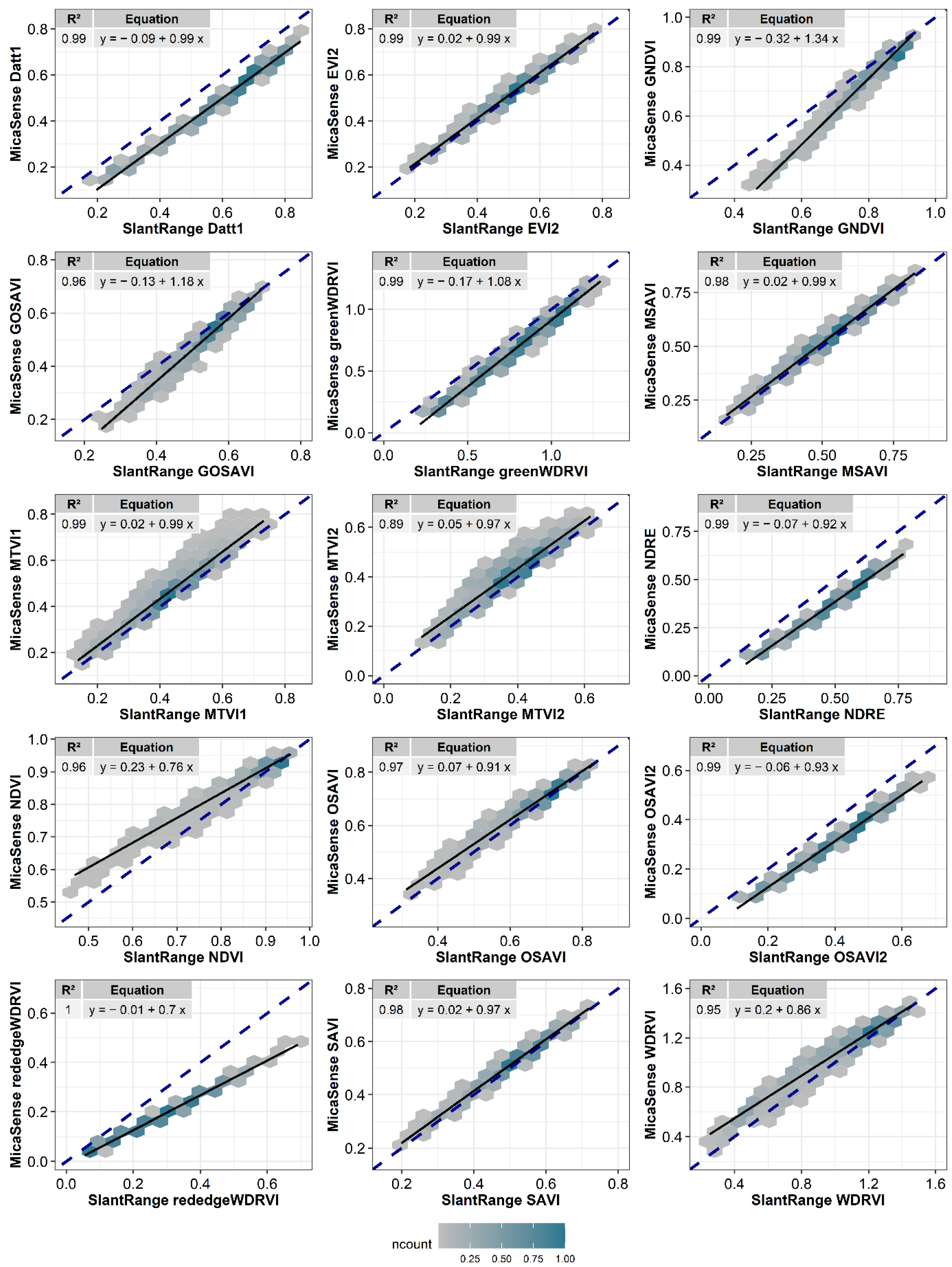
3.1. PROSAIL Model for Intercalibration of VIs Derived from Different Multispectral Sensors

The outputs of the linear regressions analysis for each VI of interest (see Table 2), as calculated from PROSAIL model simulation considering the specific spectral response function of the two sensors (y-the MicaSense VIs and x-the SlantRange VIs), are reported in Figure 2. EVI2, MSAVI, and SAVI were the three VIs with the slope values closest to 1 and intercept values closest to 0 (Figure 2). The slope values of these VIs were 0.99 for EVI2, 0.99 for MSAVI, and 0.97 for SAVI, while the intercept was respectively 0.02 for EVI2, 0.02 for MSAVI, and 0.02 for SAVI. OSAVI had a similar relation (slope: 0.91) but demonstrated higher variability at VI values lower than 0.6. Datt1, NDRE, and OSAVI2 had a relationship between the two sensors with a slope close to 1 but they displayed a different intercept, indicating an offset of the SlantRange sensor due to the underestimation of the VI compared to MicaSense (Figure 2). A slope close to 1, associated with a high variability for the whole range of VI values, was observed for MTVI1 (slope: 1) and MTVI2 (0.97). GNDVI, GOSAVI, greenWDRVI, and NDVI illustrated, instead, the highest differences between the two sensors at the lowest values of VI. On the contrary, rededgeWDRVI demonstrated the highest differences at high VI values.

3.2. Importance of Variables in Machine Learning Models

The importance of the random forest (RF) models’ variables for crop trait estimations and for yield prediction are illustrated in Figure 3. The analysis of variables’ importance for the RF models was evaluated by drop-out loss of the RMSE for each variable, compared to the full model [85,86]. The phenological stage (“Stage”) was the most important variable for estimating plant height, green leaf biomass, and standing biomass (Figure 3). For crop trait estimations, the two most important VIs were NDVI and MTVI1 for light interception, rededgeWDRVI and NDVI for plant height, and greenWDRVI and GNDVI for green leaf biomass and standing biomass. For yield prediction using VIs peaks values, the most important VIs (with a median of RMSE loss greater than 0) were greenWDRVI, NDVI, WDRVI, GNDVI, and MTVI2 (Figure 3) and the peak values of these five VIs will therefore be used for RF modelling.

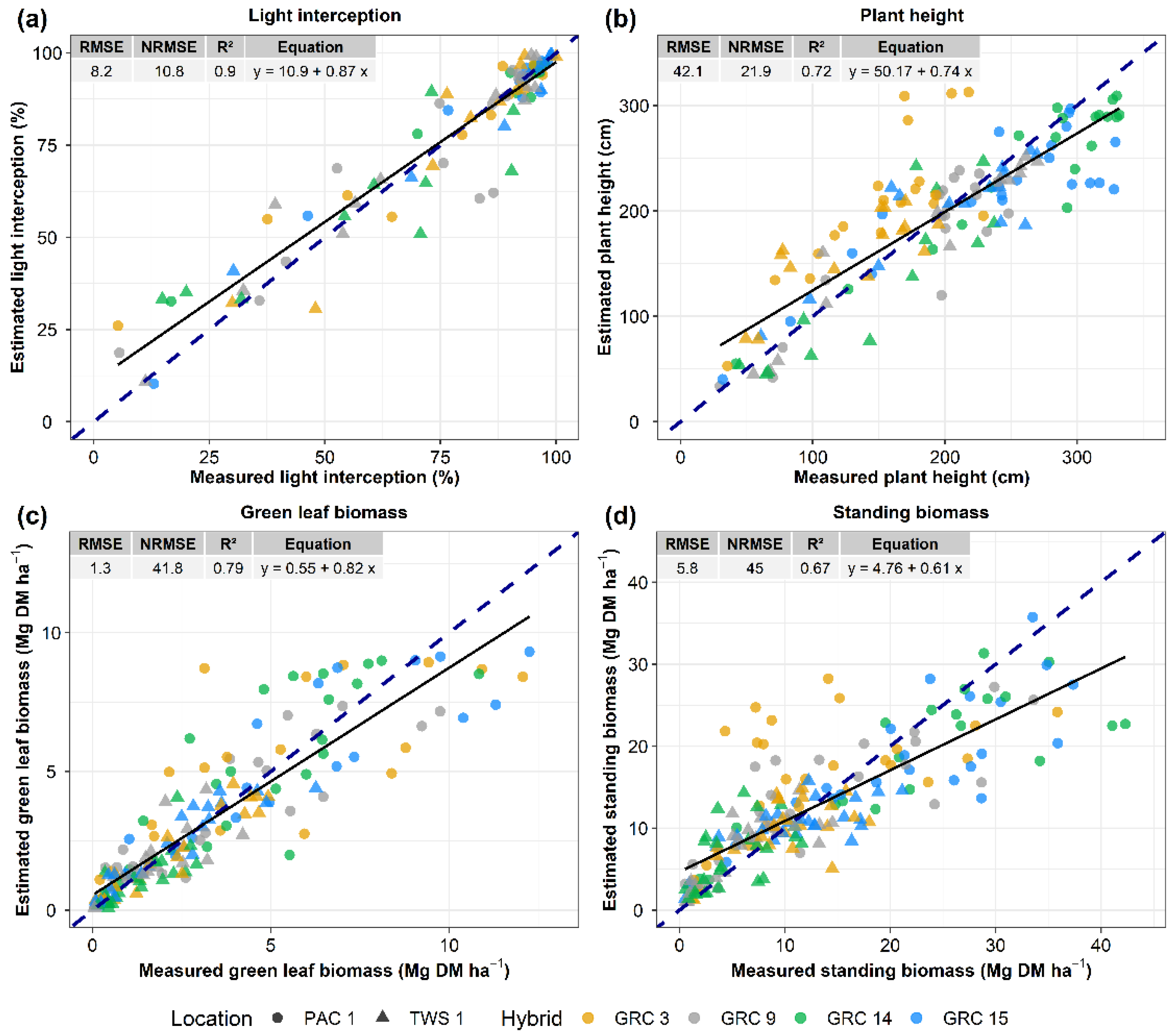
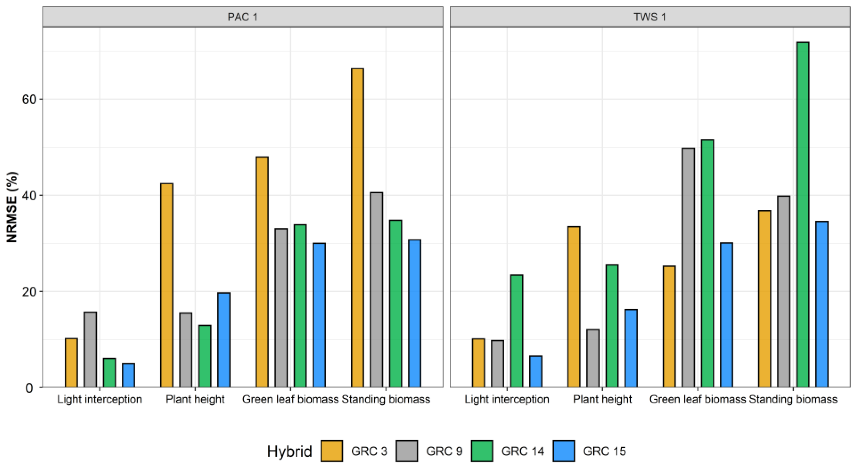
3.3. Machine Learning Model for Crop Traits Estimation

The crop trait distribution of contrasting Miscanthus hybrids, measured at two locations, is illustrated in Figure 4. The frequency distribution of the traits (light interception, plant height, green leaf biomass, and standing biomass), which values were used for training and testing the models, demonstrated that lower values were recorded in TWS 1 than in PAC 1 (Figure 4). For light interception, the range was from 5.2% to 100% in TWS 1 and PAC 1, and the mean was 58% in TWS 1 and 81.5% in PAC 1. The mean of plant height was 211 cm in PAC 1 and 147 cm in TWS 1, with the range from 28 cm to 344 cm and from 22 cm to 280 cm in PAC 1 and TWS 1, respectively. The range and the mean of green leaf biomass were from 0.14 Mg DM ha−1 to 14.5 Mg DM ha−1 and 5 Mg DM ha−1 in PAC 1 and from 0.05 Mg DM ha−1 to 6.3 Mg DM ha−1 and 1.5 Mg DM ha−1 in TWS 1. For standing biomass, the range was from 0.5 Mg DM ha−1 to 46.4 Mg DM ha−1 in PAC 1 and from 0.5 Mg DM ha−1 to 21.1 Mg DM ha−1 in TWS 1, and the mean was 8 Mg DM ha−1 in TWS 1 and 18.9 Mg DM ha−1 in PAC 1.
Overall, the RF model estimated crop traits with good model performance (Figure 5 and Figure 6). Among the crop traits, light interception was estimated with the greatest accuracy (NRMSE of 10.9%; Figure 5). High model accuracy was also achieved for the estimation of plant height (21.8% NRMSE), while the lowest model accuracies were observed for green leaf biomass and standing biomass (42.2% and 45.3% of NRMSE, respectively; Figure 5). For these last parameters, the RF model demonstrated good accuracy from low to intermediate values, while above values of 5 Mg DM ha−1 of green leaf biomass and 20 Mg DM ha−1 of standing biomass the model performances dropped. The NRMSE performance metrics for each location and hybrid are reported in Figure 6. Generally, no relevant differences were observed between the two locations (Figure 6). In PAC 1, the GRC 3 hybrid demonstrated the worst performance for green leaf biomass, for standing biomass, and for plant height, while in TWS 1, the GRC 14 hybrid demonstrated the worst performance for all the crop traits considered, except for plant height.

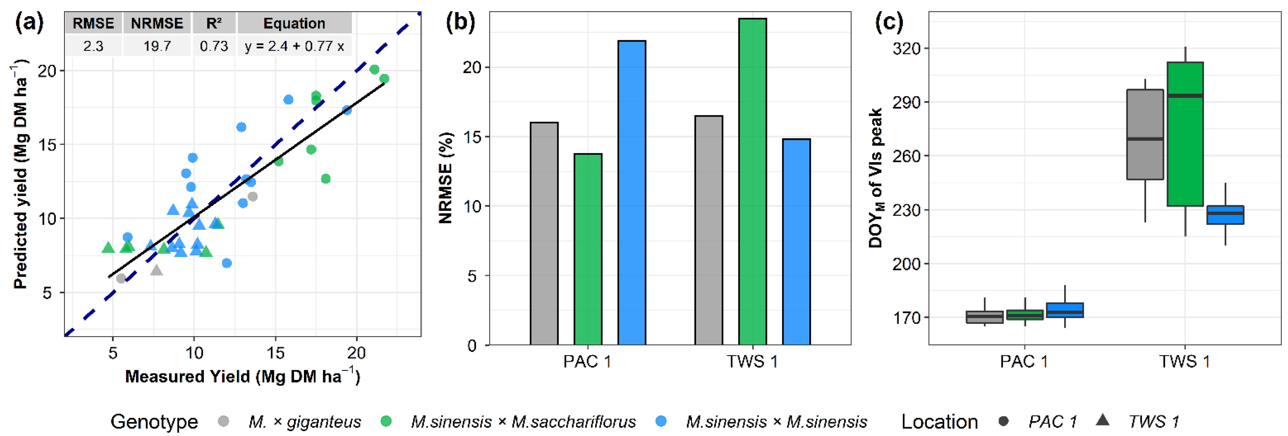
3.4. Machine Learning Model for Yield Prediction

The frequency distribution of yield measured for the 14 Miscanthus hybrids in PAC 1 and TWS 1 is provided in Figure 7. On average, the yield of Miscanthus was higher in PAC 1 than in TWS 1. In PAC 1, the highest yield was recorded by M. sin × M. sac (a mean of 18.3 Mg DM ha−1). M. sin × M. sin productivity averaged 11.3 Mg DM ha−1, while M. giganteus was less productive (mean of 9.6 Mg DM ha−1). In TWS 1, the highest yield was recorded by M. sin × M. sin (mean of 9.4 Mg DM ha−1). M. sin × M. sac productivity averaged 8.2 Mg DM ha−1 while M. giganteus was less productive (mean of 6.6 Mg DM ha−1). The RF model, trained and tested with the yield values reported in Figure 7, enabled a reliable prediction of Miscanthus yield for all hybrids, using the peak derived from the complete time series of VIs (Figure 8). The RF model obtained a RMSE value of 2.3 Mg DM ha−1 and a NRMSE value of 19.7% (Figure 8a). In PAC 1, M. sin × M. sac demonstrated the lowest NRMSE value, while M. sin × M. sin demonstrated the highest NRMSE value. On the contrary, in TWS 1, M. sin × M. sin demonstrated the lowest NRMSE value while M. sin × M. sac demonstrated the highest NRMSE value (Figure 8b). The modified days of the year (DOYM) of the peak of the Vis (greenWDRVI, NDVI, WDRVI, GNDVI, and MTVI2) are reported in Figure 8c. On average, the VIs reached the peak earlier in PAC 1 (172 DOYM–20 June) than in TWS 1 (DOYM 232–19 August). In PAC 1, all hybrids reached the peak at the same time, while in TWS 1, all M. sin × M. sin hybrids were the earliest to reach the peak (228 DOYM-15th August), while M. sin × M. sac hybrids and M. × giganteus reached the peak along a wide timespan ranging from the end of September until mid-November (Figure 8c).

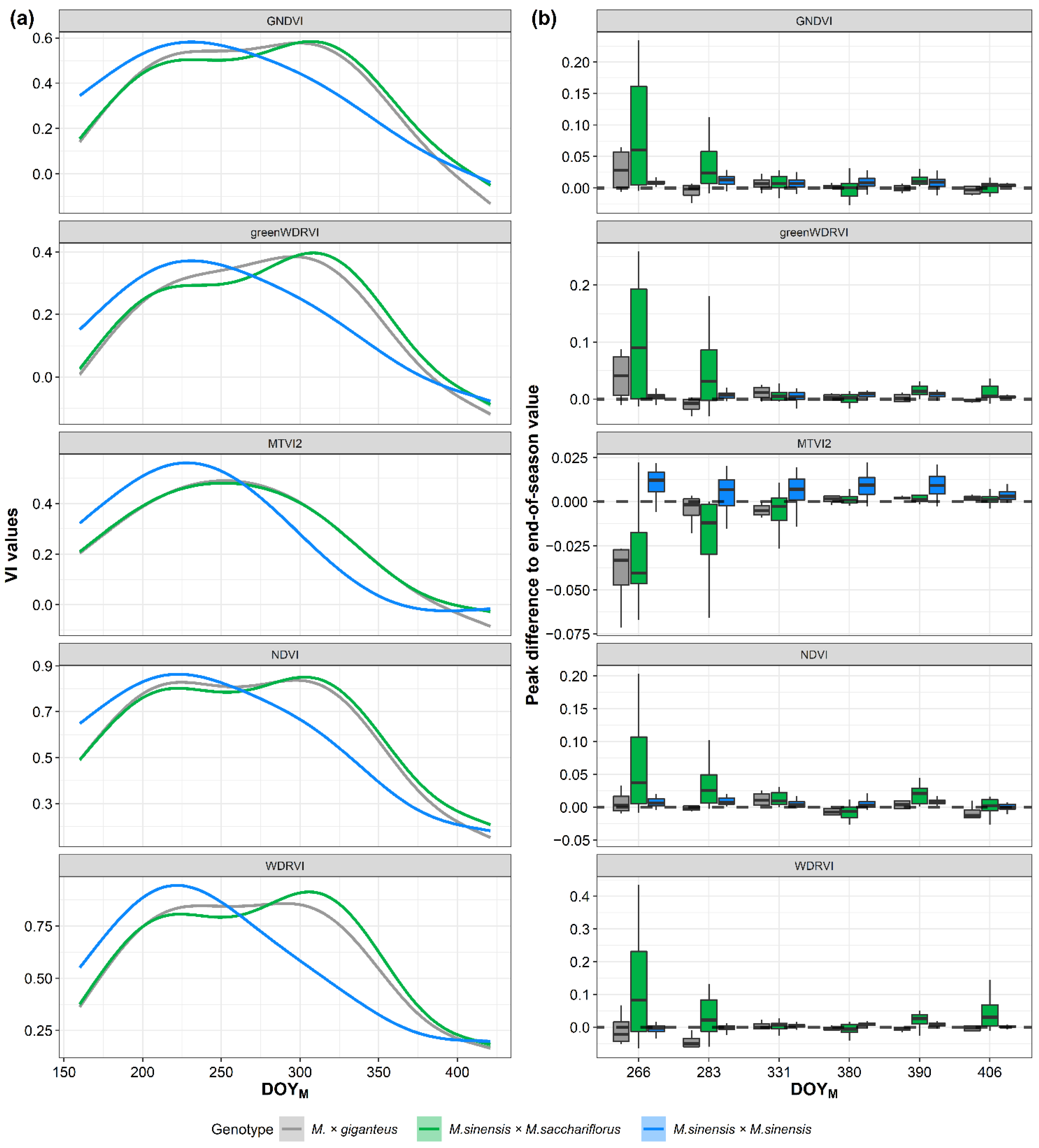
3.5. Time Series of VIs and Yield Prediction Analysis

The complete time series of the five VIs identified as the most important for yield prediction (see Section 3.2 and Figure 3) are reported in Figure 9a for PAC 1 and Figure 10a for TWS 1. In PAC 1, all VIs values recorded throughout the growth of Miscanthus were the highest for M. sin × M. sac and the lowest for M. giganteus (Figure 9a), following the same order of the mean yield measured in the field (Figure 7). In TWS 1, a similar time series of all the Vis were recorded for the M. sin × M. sac and M. giganteus (Figure 10a). In particular, the peaks of M. sin × M. sac and of M. giganteus were reached later than that of M. sin × M. sin, as illustrated in Figure 8c. The variation throughout the season of the peak, derived by fitting the VIs via the generalized additive model (GAM), are displayed in Figure 9b for PAC 1 and Figure 10b for TWS 1. In PAC 1, the difference between the value of the peak derived from the complete time series of VIs and the value of the peak derived from the partial time series of VIs is the lowest (close to zero) after the 302 DOYM (end-October). Before this date, the peaks’ differences are lower for M. sin × M. sin than M. sin × M. sac and M. giganteus (Figure 9b). In TWS 1, the difference between the value of the peak derived from the complete time series of VIs and the value of the peak derived from the partial time series of VIs is lowest after 331 DOYM (end-November). As for PAC 1, the peaks differences are lower for M. sin × M. sin than M. giganteus and M. sin × M. sac (Figure 10b) in TWS 1 before 331 DOYM. The timeline of the performance of the RF model tested with the VIs peak from partial time series is reported in Figure 11. In PAC 1, the NRMSE decreased until 302 DOYM for M. giganteus and M. sin × M. sac while for M. sin × M. sin, it remained stable for all UAV flights performed from 175 DOYM onward. In TWS 1, no relevant differences in NRMSE were observed between the UAV flights performed from 266 DOYM onward.

4. Discussion

The use of UAV-based remote sensing provides a great potential for high-throughput phenotyping (HTP) at the plot scale, with applications in both breeding and in estimating the quality and quantity of the biomass needed for optimising downstream management of biomass fluxes. In this study, vegetation indices (VIs) and their peak were derived from unmanned aerial vehicles’ (UAVs) mounted multispectral sensors to estimate crop traits (light interception, plant height, green leaf biomass, and standing biomass), and to predict the final harvestable yield of novel Miscanthus hybrids and common M. × giganteus grown at two sites (Italy and UK).

4.1. The Importance of VIs Intercalibration Procedure for Multi-Sensor Interoperability

Intercalibrating the VIs of multi-sensors is relevant for remote sensing crop monitoring [54], particularly when the objective is to build models to estimate crop traits or to predict yield, and when sensors with different spectral characteristics are used. Indeed, the models might not reach the same accuracy if the VIs are calculated with sensors with different spectral band characteristics. The spectral signatures simulated from the PROSAIL model were used in this study to intercalibrate Vis, calculated from two common multispectral cameras (MicaSense RedEdge-MX and SlantRange 4P). Ideally, the VIs from any sensor can be then intercalibrated against the VIs of a selected reference sensor. This intercalibration approach is commonly adopted for VIs obtained from different satellites, [59] but, to our knowledge, this is the first time that such an approach is applied to UAV multispectral sensors. The PROSAIL model was used to simulate the canopy reflectance based on the value of specific Miscanthus traits, such as LAI, chlorophyll content, dry matter content, relative equivalent water thickness, leaf inclination distribution, and two site-specific values: solar zenith angle and relative azimuth angle. This approach was applied to the values of 15 VIs. EVI2, MSAVI, and SAVI were the three VIs with the closest 1:1 relation, which indicates that these VIs have a very low sensitivity to the spectral characteristics of the two sensors used in the present work. Similar results with no need for intercalibration for the same VIs were reported by Li et al. [88], comparing ETM+ and OLI satellite imageries. However, the other VIs evaluated in this study (Datt1, GNDVI, GOSAVI, greenWDRVI, MTVI1, MTVI2, NDRE, NDVI, OSAVI, OSAVI2, rededgeWDRVI, and WDRVI) demonstrated a higher sensitivity to sensor characteristics, underlining the importance of intercalibrating VIs for multi-sensor interoperability. In particular, the VIs based on green and red-edge bands demonstrated a higher variation than the VIs based on the red band, at all ranges of values. These differences are explained by the differences in the spectral characteristics of MicaSense and SlantRange in the green and red-edge bands. In particular, the SlantRange sensor has a broader green FWHM (100 nm) and a different central wavelength (710 nm) of the red edge compared to the MicaSense sensor (green FWHM: 27 nm and red edge central wavelength: 717 nm). This difference was already reported to cause considerable signal differences in other studies [89,90].
This study highlighted the importance of intercalibrating different multispectral sensors to increase interoperability in remote sensing. Kim et al. [91] and Villaescusa-Nadal et al. [92] reported that the use of linear regression equations to intercalibrate multi-sensors contributes to significantly correct (up to 50%) the effects of different spectral characteristics on VIs. However, it would be interesting to validate this procedure by flying simultaneously on the same field with two UAV sensors, comparing the values of the VIs with and without the intercalibration procedure, in order to evaluate the improvement in terms of VIs compatibility and multi-sensor interoperability. In fact, even if the spectral characteristics of the multispectral sensor are the factor that influences the compatibility of the VIs of different sensors the most [49], other factors cause differences of Vis, such as the atmospheric conditions during acquisition [48]. In the UAV images acquisitions, the changing light and meteorological conditions during the flights can affect the quality of the spectral data [65]. Therefore, this procedure is limited by other factors that cannot be considered by applying a simulated regression coefficient. However, using equations that are able to intercalibrate VIs derived by multiple multispectral sensors can reduce differences in Vis, improving crop monitoring and modelling for estimation of crop traits and prediction of yield.

4.2. Estimating Miscanthus Traits with Machine Learning

This study estimated Miscanthus traits using the random forest (RF) machine learning algorithm. The RF model was trained with the data collected on three novel seed-based Miscanthus hybrids and the common rhizome-based genotype M. × giganteus, at two contrasting locations (North-West Italy and Mid-West Wales). The RF algorithm, using 15 common VIs, successfully estimated crop traits, solving the non-linear responses between VIs and crop traits observed by Li et al. [28] for other perennial crops. The estimation of the crop traits from the time series of VIs acquired by UAV-based remote sensing can generate more data useful to calibrate existing Miscanthus crop models and to re-fine these models for novel Miscanthus hybrids in contrasting environments. The crop trait estimated with the greatest accuracy was light interception, which demonstrated a RMSE of 8.4%, the accuracy being especially good at high values of light interception (Figure 5). This result is in agreement with Guillen-Climent et al. [93], who found that the fraction of intercepted photosynthetically active radiation (fIPAR) was successfully estimated by a ML algorithm. Upreti et al. [30] found similar values of NRMSE (12.06% ) using the RF tree bagger approach for estimating the fraction of absorbed photosynthetically active radiation (fAPAR) of durum wheat. Good model accuracy was also achieved for plant height estimation (RMSE = 42 cm and NRMSE = 21.8%; Figure 5). A similar RMSE value (41 cm) was found by Han et al. [31] for plant height estimation of maize using the crop surface model, and by Tao et al. [94] (NRMSE = 21.2%) in the estimation of plant height of winter wheat using UAV hyperspectral images. The worst model accuracy was found for the green leaf biomass and standing biomass, with 1.3 Mg DM ha−1 and 5.8 Mg DM ha−1 of RMSE, respectively (Figure 5). However, for these parameters, the model demonstrated good accuracy from low to intermediate values, while, above values of 5 Mg DM ha−1 of green leaf biomass and 20 Mg DM ha−1 of standing biomass, the model performance dropped. The model could be affected by errors in the estimation in these intervals due to the fewer data used to train the model [95]; in fact, most of them were collected in PAC 1 (Figure 4). The different levels of accuracy of the models in estimating light interception and plant height compared to green leaf biomass and standing biomass could also be related to the period in which the measurements were taken and to the response of VIs during senescence. Field measurements of light interception and plant height were carried out in each environment from emergence until they peaked, which explains their good model accuracy. Estimation of crop traits with data coming from single UAV flights across the growing seasons is particularly affected after biomass reaches its maximum value in autumn. After biomass peak, with the start of the senescence period, the values of VIs start to decrease (Figure 9a and Figure 10a) [96], while Miscanthus green leaf biomass and standing biomass values remained stable or slightly decreased during this period. The difference of rate of decrease between the VIs and crop traits during senescence is a key aspect to consider in remote sensing estimation of crop traits. The importance of the senescence stage in the crop traits estimation is confirmed by the results on the variables’ importance (Figure 3). Indeed, the phenological variable “Stage” was the most important variable in the estimation of plant height, green leaf biomass, and standing biomass. The plant height of the GRC 3 (a M. sin × M. sin planted at high density) were poorly estimated, and this could be due to its canopy architecture and flowering time. The M. sin × M. sin hybrid has many distinguishable stems flowering (where plant height is measured), but its leaves are particularly curved and attached along the stem at a lower height than M. sin × M. sac. In addition, this genotype was transplanted at higher densities (3 plants m−2) and flowered earlier (end of August) compared to other genotypes, which flowered in early autumn. This more “prostrate” canopy architecture (with a higher stem segment between inflorescences and bent leaves) introduced noise in the plant height estimation from UAVs [97], since most of the reflectance comes from bent leaf mass. This noise caused by changes in plant architecture and the onset of flower can be seen in the NRMSE values of the RF models at the PAC 1 site (Figure 6). In fact, the earlier a genotype with prostrate architecture flowers, the worse is the estimation of plant height and biomass from an UAV.

4.3. Yield Prediction Using Machine Learning and Peak of VIs

The random forest (RF) trained with the peak derived from complete time series of five VIs acquired by UAVs was able to predict the yield of the 14 Miscanthus hybrids. The peak value of greenWDRVI, NDVI, WDRVI, GNDVI, and MTVI2 resulted the most important features for RF modelling, as derived from previous analysis (see Section 3.2, Figure 3). The RF model accurately predicted the yield, with 2.3 Mg DM ha−1 of RMSE and 19.7% NRMSE (Figure 8a). The peak for Miscanthus hybrids occurs on average in mid-summer and early autumn in southern/warm (Italy) and northern/cold (UK) locations, respectively. The importance of the peak as land surface phenology (LSP) descriptors for yield prediction was already reported by Prasad et al. [98], who found that the peak had the highest correlation with cotton yield prediction compared to other LSP descriptors. Similar results were reported by Montazeaud et al. [47], who found a high correlation between the peak of NDVI and the yield, and by Liu et al. [17], who found that the EVI2 peak was a good predictor of grain yield. Among the VIs used in the RF model, the peak of the VIs based on the green band as GNDVI and greenWDRVI (Figure 3) were the most important variables for predicting not only Miscanthus yield at harvest, but also in estimating standing biomass and green leaf biomass during the growing season (Figure 4). Similar results for GNDVI were found in switchgrass and other warm-season perennial grasses [26]. In order to assess the capability of the model to predict the yield months before harvest (i.e., using only early season UAV acquisition and not waiting to perform UAV monitoring during the entire crop season), the RF model was calculated using the peak derived from the partial time series of Vis, and performance analysed. In the UK, the RF model accurately predicted the yield five months before harvest for all Miscanthus hybrids. In Italy, the yield of the M. sin × M. sin hybrids can be predicted with good accuracy seven months before harvest while M. giganteus and M. sin × M. sac hybrids required more time, as a good accuracy was obtained 3–4 months before harvest. This capability of the model to predict yield months before harvest is possible if no damage to plants later in the season occurs, thus considering a steady development process. Given the good accuracy achieved by the RF model even when peak value is assessed on a limited number of data (see Section 3.5, Figure 11), this approach can be considered as a suitable method to predict yield several months before harvest. However, it is possible that no time series analyses (i.e., a complete series of dense observation from sowing to harvest) are required, and the 5 VIs values could be used directly as inputs for yield prediction modelling, if the UAV data is acquired in the range of expected peak occurrence. This opportunity was also reported for switchgrass [26] using multispectral images acquired from multiple UAV flights, underlying the possibility of reducing the number of multispectral observations (e.g., 25 UAV flights were performed in PAC 1) to 2–3 UAV flights in proximity of the VIs’ peak period. In this context, the identification of VIs’ peak period, which is generally related to crop physiology and phenology (reaching the maximum production), is important in terms of cost (reduction of the number of observations) and of operationality of the yield prediction model. This model operability, intended as a capability of the model to accurately predict the yield some months before the harvest, is extremely relevant for improving the logistics of the biomass supply chain of Miscanthus and for supporting the improvement of crop modelling with remote sensing data.

5. Conclusions

This study demonstrated that vegetation indices (VIs) derived from unmanned aerial vehicle (UAV) multispectral images acquired in Italy and the UK can be successfully used in random forest (RF) machine learning (ML) algorithms to estimate the light interception, plant height, green leaf biomass, and standing biomass, and to predict the yield of novel Miscanthus hybrids using the peak derived from the VIs’ time series. This study evaluated the timeline of the performance of the model using peaks derived from the partial VIs’ time series, and the RF model demonstrated a good capability to predict the yield months before the harvest, both in Italy and in the UK, by using a limited number of UAV observations. In particular, the results suggested that the VIs’ values acquired during the peak period (without using the complete or partial time series) could be used directly for yield prediction, increasing the model operability. Yield prediction and high-throughput phenotyping, based on ML algorithms and on UAV remote sensing, can improve the logistics of the biomass supply chain, supporting breeding programs, and improving the crop modelling of novel Miscanthus hybrids. UAV platforms are suitable tools for HTP applications, as they enable the monitoring of small plots or field scale trials with numerous genotypes, due to their ability to capture high-resolution images. However, the satellite platforms are more suited for yield prediction, as they can collect data of many fields simultaneously and can develop applications to predict commercial yield at regional and national scales. In addition, this study reported for the first time a methodology to overcome the issue of multi-sensor interoperability among UAV multispectral sensors. The use of intercalibrating equations derived from the PROSAIL model proved to be a powerful tool to intercalibrate VIs from multi-sensors with different spectral characteristics. Although this intercalibration procedure is relevant for the upscaling of models from experimental plots to field by intercalibrating the UAV with satellites sensor characteristics, it is limited because it only considers the spectral sensor characteristics and no other factors, such as light and meteorological conditions during the flights, which may affect the quality of the spectral data and cannot be considered by applying a simulated regression coefficient.

Supplementary Materials

The following supporting information can be downloaded at: https://www.mdpi.com/article/10.3390/rs14122927/s1, Table S1. Seasonal calendar of UAV flights performed in the two locations according to the estimated phenological stages (vegetative growth and senescence).

Author Contributions

Conceptualization, G.I., M.C., A.F. and S.A.; methodology, G.I. and M.C.; software, G.I. and M.C; formal analysis, G.I.; data curation, G.I.; visualization, G.I.; investigation, G.I., M.C., J.B., A.M., H.B., E.M., C.A. and D.A.-C.; resources, J.K., L.M.T., J.C.-B., A.K. and S.A; writing—original draft preparation, G.I.; writing—review and editing, A.F., J.C.-B., M.B. and S.A.; funding acquisition, S.A. All authors have read and agreed to the published version of the manuscript.

Funding

This study is part of the GRACE project, which has received funding from the Bio-based Industries Joint Undertaking (JU) under the European Union’s Horizon 2020 research and innovation programme under grant agreement No 745012. The JU receives support from the European Union’s Horizon 2020 research and innovation programme and the Bio-based Industries Consortium.

Data Availability Statement

The data that support the findings of this work are available from the corresponding author upon reasonable request.

Conflicts of Interest

The authors declare no conflict of interest.

References

  1. Lewandowski, I.; Clifton-Brown, J.C.; Scurlock, J.M.O.; Huisman, W. Miscanthus: European Experience with a Novel Energy Crop. Biomass Bioenergy 2000, 19, 209–227. [Google Scholar] [CrossRef]
  2. Clifton-Brown, J.; Hastings, A.; Mos, M.; McCalmont, J.P.; Ashman, C.; Awty-Carroll, D.; Cerazy, J.; Chiang, Y.-C.; Cosentino, S.; Cracroft-Eley, W.; et al. Progress in Upscaling Miscanthus Biomass Production for the European Bio-Economy with Seed-Based Hybrids. GCB Bioenergy 2017, 9, 6–17. [Google Scholar] [CrossRef] [Green Version]
  3. Clifton-Brown, J.C.; Lewandowski, I.; Andersson, B.; Basch, G.; Christian, D.G.; Kjeldsen, J.B.; J⊘rgensen, U.; Mortensen, J.V.; Riche, A.B.; Schwarz, K.-U.; et al. Performance of 15 Miscanthus Genotypes at Five Sites in Europe. Agron. J. 2001, 93, 1013–1019. [Google Scholar] [CrossRef] [Green Version]
  4. Jones, M.B.; Zimmermann, J.; Clifton-Brown, J. Long-Term Yields and Soil Carbon Sequestration from Miscanthus: A Review. In Perennial Biomass Crops for a Resource-Constrained World; Springer International Publishing: Cham, Switzerland, 2016; pp. 43–49. [Google Scholar]
  5. Clifton-Brown, J.; Harfouche, A.; Casler, M.D.; Dylan Jones, H.; Macalpine, W.J.; Murphy-Bokern, D.; Smart, L.B.; Adler, A.; Ashman, C.; Awty-Carroll, D.; et al. Breeding Progress and Preparedness for Mass-scale Deployment of Perennial Lignocellulosic Biomass Crops Switchgrass, Miscanthus, Willow and Poplar. GCB Bioenergy 2019, 11, 118–151. [Google Scholar] [CrossRef] [Green Version]
  6. Lewandowski, I.; Clifton-Brown, J.; Trindade, L.M.; van der Linden, G.C.; Schwarz, K.-U.U.; Müller-Sämann, K.; Anisimov, A.; Chen, C.-L.L.; Dolstra, O.; Donnison, I.S.; et al. Progress on Optimizing Miscanthus Biomass Production for the European Bioeconomy: Results of the EU FP7 Project OPTIMISC. Front. Plant Sci. 2016, 7, 1620. [Google Scholar] [CrossRef] [Green Version]
  7. van der Cruijsen, K.; Al Hassan, M.; van Erven, G.; Dolstra, O.; Trindade, L.M. Breeding Targets to Improve Biomass Quality in Miscanthus. Molecules 2021, 26, 254. [Google Scholar] [CrossRef]
  8. Clifton-Brown, J.; Schwarz, K.-U.; Awty-Carroll, D.; Iurato, A.; Meyer, H.; Greef, J.; Gwyn, J.; Mos, M.; Ashman, C.; Hayes, C.; et al. Breeding Strategies to Improve Miscanthus as a Sustainable Source of Biomass for Bioenergy and Biorenewable Products. Agronomy 2019, 9, 673. [Google Scholar] [CrossRef] [Green Version]
  9. Hastings, A.; Mos, M.; Yesufu, J.A.; McCalmont, J.; Schwarz, K.; Shafei, R.; Ashman, C.; Nunn, C.; Schuele, H.; Cosentino, S.; et al. Economic and Environmental Assessment of Seed and Rhizome Propagated Miscanthus in the UK. Front. Plant Sci. 2017, 8, 1058. [Google Scholar] [CrossRef] [Green Version]
  10. Pancaldi, F.; Trindade, L.M. Marginal Lands to Grow Novel Bio-Based Crops: A Plant Breeding Perspective. Front. Plant Sci. 2020, 11, 227. [Google Scholar] [CrossRef] [Green Version]
  11. de Wit, A.J.W.; van Diepen, C.A. Crop Growth Modelling and Crop Yield Forecasting Using Satellite-Derived Meteorological Inputs. Int. J. Appl. Earth Obs. Geoinf. 2008, 10, 414–425. [Google Scholar] [CrossRef]
  12. Keating, B.; Carberry, P.; Hammer, G.; Probert, M.; Robertson, M.; Holzworth, D.; Huth, N.; Hargreaves, J.N.; Meinke, H.; Hochman, Z.; et al. An Overview of APSIM, a Model Designed for Farming Systems Simulation. Eur. J. Agron. 2003, 18, 267–288. [Google Scholar] [CrossRef] [Green Version]
  13. MacKerron, D.K.L.; Haverkort, A.J. (Eds.) Decision Support Systems in Potato Production; Wageningen Academic Publishers: Wageningen, The Netherlands, 2004; ISBN 978-90-76998-30-5. [Google Scholar]
  14. Hastings, A.; Clifton-Brown, J.; Wattenbach, M.; Mitchell, C.P.; Smith, P. The Development of MISCANFOR, a New Miscanthus Crop Growth Model: Towards More Robust Yield Predictions under Different Climatic and Soil Conditions. GCB Bioenergy 2009, 1, 154–170. [Google Scholar] [CrossRef]
  15. Zhang, B.; Hastings, A.; Clifton-Brown, J.C.; Jiang, D.; Faaij, A.P.C. Modeled Spatial Assessment of Biomass Productivity and Technical Potential of Miscanthus × Giganteus, Panicum Virgatum L., and Jatropha on Marginal Land in China. GCB Bioenergy 2020, 12, 328–345. [Google Scholar] [CrossRef] [Green Version]
  16. Henner, D.N.; Hastings, A.; Pogson, M.; McNamara, N.P.; Davies, C.A.; Smith, P. PopFor: A New Model for Estimating Poplar Yields. Biomass Bioenergy 2020, 134, 105470. [Google Scholar] [CrossRef]
  17. Liu, J.; Shang, J.; Qian, B.; Huffman, T.; Zhang, Y.; Dong, T.; Jing, Q.; Martin, T. Crop Yield Estimation Using Time-Series MODIS Data and the Effects of Cropland Masks in Ontario, Canada. Remote Sens. 2019, 11, 2419. [Google Scholar] [CrossRef] [Green Version]
  18. Richter, G.M.; Agostini, F.; Barker, A.; Costomiris, D.; Qi, A. Assessing On-Farm Productivity of Miscanthus Crops by Combining Soil Mapping, Yield Modelling and Remote Sensing. Biomass Bioenergy 2016, 85, 252–261. [Google Scholar] [CrossRef] [Green Version]
  19. Impollonia, G.; Croci, M.; Martani, E.; Ferrarini, A.; Kam, J.; Trindade, L.M.; Clifton-Brown, J.; Amaducci, S. Moisture Content Estimation and Senescence Phenotyping of Novel Miscanthus Hybrids Combining UAV-based Remote Sensing and Machine Learning. GCB Bioenergy 2022, 14, 639–656. [Google Scholar] [CrossRef]
  20. Potgieter, A.B.; George-Jaeggli, B.; Chapman, S.C.; Laws, K.; Suárez Cadavid, L.A.; Wixted, J.; Watson, J.; Eldridge, M.; Jordan, D.R.; Hammer, G.L. Multi-Spectral Imaging from an Unmanned Aerial Vehicle Enables the Assessment of Seasonal Leaf Area Dynamics of Sorghum Breeding Lines. Front. Plant Sci. 2017, 8, 1532. [Google Scholar] [CrossRef]
  21. Blancon, J.; Dutartre, D.; Tixier, M.-H.H.; Weiss, M.; Comar, A.; Praud, S.; Baret, F. A High-Throughput Model-Assisted Method for Phenotyping Maize Green Leaf Area Index Dynamics Using Unmanned Aerial Vehicle Imagery. Front. Plant Sci. 2019, 10, 685. [Google Scholar] [CrossRef]
  22. Antonucci, G.; Impollonia, G.; Croci, M.; Potenza, E.; Marcone, A.; Amaducci, S. Evaluating Biostimulants via High-Throughput Field Phenotyping: Biophysical Traits Retrieval through PROSAIL Inversion. Smart Agric. Technol. 2023, 3, 100067. [Google Scholar] [CrossRef]
  23. Jongschaap, R.E.E. Run-Time Calibration of Simulation Models by Integrating Remote Sensing Estimates of Leaf Area Index and Canopy Nitrogen. Eur. J. Agron. 2006, 24, 316–324. [Google Scholar] [CrossRef]
  24. Prévot, L.; Chauki, H.; Troufleau, D.; Weiss, M.; Baret, F.; Brisson, N. Assimilating Optical and Radar Data into the STICS Crop Model for Wheat. Agronomie 2003, 23, 297–303. [Google Scholar] [CrossRef] [Green Version]
  25. Ferchichi, A.; Abbes, A.B.; Barra, V.; Farah, I.R. Forecasting Vegetation Indices from Spatio-Temporal Remotely Sensed Data Using Deep Learning-Based Approaches: A Systematic Literature Review. Ecol. Inform. 2022, 68, 101552. [Google Scholar] [CrossRef]
  26. Hamada, Y.; Zumpf, C.R.; Cacho, J.F.; Lee, D.; Lin, C.-H.; Boe, A.; Heaton, E.; Mitchell, R.; Negri, M.C.; Rescia, A.; et al. Remote Sensing-Based Estimation of Advanced Perennial Grass Biomass Yields for Bioenergy. Land 2021, 10, 1221. [Google Scholar] [CrossRef]
  27. Wang, J.; Badenhorst, P.; Phelan, A.; Pembleton, L.; Shi, F.; Cogan, N.; Spangenberg, G.; Smith, K. Using Sensors and Unmanned Aircraft Systems for High-Throughput Phenotyping of Biomass in Perennial Ryegrass Breeding Trials. Front. Plant Sci. 2019, 10, 1381. [Google Scholar] [CrossRef]
  28. Li, F.; Piasecki, C.; Millwood, R.J.; Wolfe, B.; Mazarei, M.; Stewart, C.N. High-Throughput Switchgrass Phenotyping and Biomass Modeling by UAV. Front. Plant Sci. 2020, 11, 1532. [Google Scholar] [CrossRef]
  29. Jin, S.; Su, Y.; Gao, S.; Hu, T.; Liu, J.; Guo, Q. The Transferability of Random Forest in Canopy Height Estimation from Multi-Source Remote Sensing Data. Remote Sens. 2018, 10, 1183. [Google Scholar] [CrossRef] [Green Version]
  30. Upreti, D.; Huang, W.; Kong, W.; Pascucci, S.; Pignatti, S.; Zhou, X.; Ye, H.; Casa, R. A Comparison of Hybrid Machine Learning Algorithms for the Retrieval of Wheat Biophysical Variables from Sentinel-2. Remote Sens. 2019, 11, 481. [Google Scholar] [CrossRef] [Green Version]
  31. Han, L.; Yang, G.; Dai, H.; Xu, B.; Yang, H.; Feng, H.; Li, Z.; Yang, X. Modeling Maize Above-Ground Biomass Based on Machine Learning Approaches Using UAV Remote-Sensing Data. Plant Methods 2019, 15, 10. [Google Scholar] [CrossRef] [Green Version]
  32. Adam, E.; Mutanga, O.; Abdel-Rahman, E.M.; Ismail, R. Estimating Standing Biomass in Papyrus ( Cyperus Papyrus L.) Swamp: Exploratory of in Situ Hyperspectral Indices and Random Forest Regression. Int. J. Remote Sens. 2014, 35, 693–714. [Google Scholar] [CrossRef]
  33. Verrelst, J.; Malenovský, Z.; Van der Tol, C.; Camps-Valls, G.; Gastellu-Etchegorry, J.-P.; Lewis, P.; North, P.; Moreno, J. Quantifying Vegetation Biophysical Variables from Imaging Spectroscopy Data: A Review on Retrieval Methods. Surv. Geophys. 2019, 40, 589–629. [Google Scholar] [CrossRef] [Green Version]
  34. Wang, L.; Zhou, X.; Zhu, X.; Dong, Z.; Guo, W. Estimation of Biomass in Wheat Using Random Forest Regression Algorithm and Remote Sensing Data. Crop J. 2016, 4, 212–219. [Google Scholar] [CrossRef] [Green Version]
  35. Guo, Y.; Fu, Y.; Hao, F.; Zhang, X.; Wu, W.; Jin, X.; Robin Bryant, C.; Senthilnath, J. Integrated Phenology and Climate in Rice Yields Prediction Using Machine Learning Methods. Ecol. Indic. 2021, 120, 106935. [Google Scholar] [CrossRef]
  36. Belgiu, M.; Drăguţ, L. Random Forest in Remote Sensing: A Review of Applications and Future Directions. ISPRS J. Photogramm. Remote Sens. 2016, 114, 24–31. [Google Scholar] [CrossRef]
  37. Hunt, M.L.; Blackburn, G.A.; Carrasco, L.; Redhead, J.W.; Rowland, C.S. High Resolution Wheat Yield Mapping Using Sentinel-2. Remote Sens. Environ. 2019, 233, 111410. [Google Scholar] [CrossRef]
  38. Jeong, J.H.; Resop, J.P.; Mueller, N.D.; Fleisher, D.H.; Yun, K.; Butler, E.E.; Timlin, D.J.; Shim, K.-M.; Gerber, J.S.; Reddy, V.R.; et al. Random Forests for Global and Regional Crop Yield Predictions. PLoS ONE 2016, 11, e0156571. [Google Scholar] [CrossRef]
  39. Marques Ramos, A.P.; Prado Osco, L.; Elis Garcia Furuya, D.; Nunes Gonçalves, W.; Cordeiro Santana, D.; Pereira Ribeiro Teodoro, L.; Antonio da Silva Junior, C.; Fernando Capristo-Silva, G.; Li, J.; Henrique Rojo Baio, F.; et al. A Random Forest Ranking Approach to Predict Yield in Maize with Uav-Based Vegetation Spectral Indices. Comput. Electron. Agric. 2020, 178, 105791. [Google Scholar] [CrossRef]
  40. Senthilnath, J.; Dokania, A.; Kandukuri, M.; Ramesh, K.N.; Anand, G.; Omkar, S.N.N. Detection of Tomatoes Using Spectral-Spatial Methods in Remotely Sensed RGB Images Captured by UAV. Biosyst. Eng. 2016, 146, 16–32. [Google Scholar] [CrossRef]
  41. de Beurs, K.M.; Henebry, G.M. Land Surface Phenology and Temperature Variation in the International Geosphere-Biosphere Program High-Latitude Transects. Glob. Chang. Biol. 2005, 11, 779–790. [Google Scholar] [CrossRef]
  42. Ji, Z.; Pan, Y.; Zhu, X.; Wang, J.; Li, Q. Prediction of Crop Yield Using Phenological Information Extracted from Remote Sensing Vegetation Index. Sensors 2021, 21, 1406. [Google Scholar] [CrossRef]
  43. Meroni, M.; d’Andrimont, R.; Vrieling, A.; Fasbender, D.; Lemoine, G.; Rembold, F.; Seguini, L.; Verhegghen, A. Comparing Land Surface Phenology of Major European Crops as Derived from SAR and Multispectral Data of Sentinel-1 and -2. Remote Sens. Environ. 2021, 253, 112232. [Google Scholar] [CrossRef] [PubMed]
  44. Guo, Y.; Fu, Y.H.; Chen, S.; Robin Bryant, C.; Li, X.; Senthilnath, J.; Sun, H.; Wang, S.; Wu, Z.; de Beurs, K. Integrating Spectral and Textural Information for Identifying the Tasseling Date of Summer Maize Using UAV Based RGB Images. Int. J. Appl. Earth Obs. Geoinf. 2021, 102, 102435. [Google Scholar] [CrossRef]
  45. Yang, Q.; Shi, L.; Han, J.; Yu, J.; Huang, K. A near Real-Time Deep Learning Approach for Detecting Rice Phenology Based on UAV Images. Agric. For. Meteorol. 2020, 287, 107938. [Google Scholar] [CrossRef]
  46. de Beurs, K.M.; Henebry, G.M. Spatio-Temporal Statistical Methods for Modelling Land Surface Phenology. In Phenological Research; Springer: Dordrecht, The Netherlands, 2010; pp. 177–208. [Google Scholar]
  47. Montazeaud, G.; Karatoğma, H.; Özturk, I.; Roumet, P.; Ecarnot, M.; Crossa, J.; Özer, E.; Özdemir, F.; Lopes, M.S. Predicting Wheat Maturity and Stay–Green Parameters by Modeling Spectral Reflectance Measurements and Their Contribution to Grain Yield under Rainfed Conditions. F. Crop. Res. 2016, 196, 191–198. [Google Scholar] [CrossRef] [Green Version]
  48. Psomiadis, E.; Dercas, N.; Dalezios, N.R.; Spiropoulos, N.V. Evaluation and Cross-Comparison of Vegetation Indices for Crop Monitoring from Sentinel-2 and Worldview-2 Images. In Remote Sensing for Agriculture, Ecosystems, and Hydrology XIX; Neale, C.M., Maltese, A., Eds.; SPIE: Bellingham, WA, USA, 2017; p. 79. [Google Scholar]
  49. Théau, J.; Sankey, T.T.; Weber, K.T. Multi-Sensor Analyses of Vegetation Indices in a Semi-Arid Environment. GISci. Remote Sens. 2010, 47, 260–275. [Google Scholar] [CrossRef] [Green Version]
  50. Hoque, M.A.-A.; Phinn, S. Methods for Linking Drone and Field Hyperspectral Data to Satellite Data. In Fundamentals, Sensor Systems, Spectral Libraries, and Data Mining for Vegetation; CRC Press: Boca Raton, FL, USA, 2018; pp. 321–354. [Google Scholar]
  51. Emilien, A.-V.; Thomas, C.; Thomas, H. UAV & Satellite Synergies for Optical Remote Sensing Applications: A Literature Review. Sci. Remote Sens. 2021, 3, 100019. [Google Scholar] [CrossRef]
  52. Brown, M.E.; Pinzon, J.E.; Didan, K.; Morisette, J.T.; Tucker, C.J. Evaluation of the Consistency of Long-Term NDVI Time Series Derived from AVHRR, SPOT-Vegetation, SeaWiFS, MODIS, and Landsat ETM+ Sensors. IEEE Trans. Geosci. Remote Sens. 2006, 44, 1787–1793. [Google Scholar] [CrossRef]
  53. Gallo, K.; Ji, L.; Reed, B.; Eidenshink, J.; Dwyer, J. Multi-Platform Comparisons of MODIS and AVHRR Normalized Difference Vegetation Index Data. Remote Sens. Environ. 2005, 99, 221–231. [Google Scholar] [CrossRef] [Green Version]
  54. Meroni, M.; Atzberger, C.; Vancutsem, C.; Gobron, N.; Baret, F.; Lacaze, R.; Eerens, H.; Leo, O. Evaluation of Agreement Between Space Remote Sensing SPOT-VEGETATION FAPAR Time Series. IEEE Trans. Geosci. Remote Sens. 2013, 51, 1951–1962. [Google Scholar] [CrossRef]
  55. She, X.; Zhang, L.; Cen, Y.; Wu, T.; Huang, C.; Baig, M.H.A. Comparison of the Continuity of Vegetation Indices Derived from Landsat 8 OLI and Landsat 7 ETM+ Data among Different Vegetation Types. Remote Sens. 2015, 7, 13485–13506. [Google Scholar] [CrossRef] [Green Version]
  56. Teillet, P.; Fedosejevs, G.; Barker, J.; Miskey, C.; Bannari, A. Spectral Simulations of Vegetation Indices in the Context of Landsat Data Continuity. In Proceedings of the 2006 IEEE International Symposium on Geoscience and Remote Sensing, Denver, CO, USA, 31 July–4 August 2006; pp. 1784–1787. [Google Scholar]
  57. Teillet, P.M.; Ren, X. Spectral Band Difference Effects on Vegetation Indices Derived from Multiple Satellite Sensor Data. Can. J. Remote Sens. 2008, 34, 159–173. [Google Scholar]
  58. Laliberte, A.S.; Goforth, M.A.; Steele, C.M.; Rango, A. Multispectral Remote Sensing from Unmanned Aircraft: Image Processing Workflows and Applications for Rangeland Environments. Remote Sens. 2011, 3, 2529–2551. [Google Scholar] [CrossRef] [Green Version]
  59. van Leeuwen, W.J.D.; Orr, B.J.; Marsh, S.E.; Herrmann, S.M. Multi-Sensor NDVI Data Continuity: Uncertainties and Implications for Vegetation Monitoring Applications. Remote Sens. Environ. 2006, 100, 67–81. [Google Scholar] [CrossRef]
  60. Baret, F.; Jacquemoud, S.; Guyot, G.; Leprieur, C. Modeled Analysis of the Biophysical Nature of Spectral Shifts and Comparison with Information Content of Broad Bands. Remote Sens. Environ. 1992, 41, 133–142. [Google Scholar] [CrossRef]
  61. Jacquemoud, S.; Verhoef, W.; Baret, F.; Bacour, C.; Zarco-Tejada, P.J.; Asner, G.P.; François, C.; Ustin, S.L. PROSPECT+SAIL Models: A Review of Use for Vegetation Characterization. Remote Sens. Environ. 2009, 113, S56–S66. [Google Scholar] [CrossRef]
  62. Berger, K.; Atzberger, C.; Danner, M.; D’Urso, G.; Mauser, W.; Vuolo, F.; Hank, T.; D’Urso, G.; Mauser, W.; Vuolo, F.; et al. Evaluation of the PROSAIL Model Capabilities for Future Hyperspectral Model Environments: A Review Study. Remote Sens. 2018, 10, 85. [Google Scholar] [CrossRef] [Green Version]
  63. Verrelst, J.; Camps-Valls, G.; Muñoz-Marí, J.; Rivera, J.P.; Veroustraete, F.; Clevers, J.G.P.W.; Moreno, J. Optical Remote Sensing and the Retrieval of Terrestrial Vegetation Bio-Geophysical Properties—A Review. ISPRS J. Photogramm. Remote Sens. 2015, 108, 273–290. [Google Scholar] [CrossRef]
  64. Tejera, M.D.; Miguez, F.E.; Heaton, E.A. The Older Plant Gets the Sun: Age-Related Changes in Miscanthus × Giganteus Phenology. GCB Bioenergy 2021, 13, 4–20. [Google Scholar] [CrossRef]
  65. Guo, Y.; Senthilnath, J.; Wu, W.; Zhang, X.; Zeng, Z.; Huang, H. Radiometric Calibration for Multispectral Camera of Different Imaging Conditions Mounted on a UAV Platform. Sustainability 2019, 11, 978. [Google Scholar] [CrossRef] [Green Version]
  66. Datt, B. Remote Sensing of Water Content in Eucalyptus Leaves. Aust. J. Bot. 1999, 47, 909. [Google Scholar] [CrossRef]
  67. Miura, T.; Yoshioka, H.; Fujiwara, K.; Yamamoto, H. Inter-Comparison of ASTER and MODIS Surface Reflectance and Vegetation Index Products for Synergistic Applications to Natural Resource Monitoring. Sensors 2008, 8, 2480–2499. [Google Scholar] [CrossRef] [PubMed] [Green Version]
  68. Gitelson, A.A.; Kaufman, Y.J.; Merzlyak, M.N. Use of a Green Channel in Remote Sensing of Global Vegetation from EOS-MODIS. Remote Sens. Environ. 1996, 58, 289–298. [Google Scholar] [CrossRef]
  69. Sripada, R.P.; Heiniger, R.W.; White, J.G.; Meijer, A.D. Aerial Color Infrared Photography for Determining Early In-Season Nitrogen Requirements in Corn. Agron. J. 2006, 98, 968–977. [Google Scholar] [CrossRef]
  70. Gitelson, A.A. Wide Dynamic Range Vegetation Index for Remote Quantification of Biophysical Characteristics of Vegetation. J. Plant Physiol. 2004, 161, 165–173. [Google Scholar] [CrossRef] [Green Version]
  71. Qi, J.; Chehbouni, A.; Huete, A.R.; Kerr, Y.H.; Sorooshian, S. A Modified Soil Adjusted Vegetation Index. Remote Sens. Environ. 1994, 48, 119–126. [Google Scholar] [CrossRef]
  72. Haboudane, D.; Miller, J.R.; Pattey, E.; Zarco-Tehada, P.J.; Strachan, I.B. Hyperspectral Vegetation Indices and Novel Algorithms for Predicting Green LAI of Crop Canopies: Modeling and Validation in the Context of Precision Agriculture. Remote Sens. Environ. 2004, 90, 337–352. [Google Scholar] [CrossRef]
  73. Gitelson, A.; Merzlyak, M.N. Quantitative Estimation of Chlorophyll-a Using Reflectance Spectra: Experiments with Autumn Chestnut and Maple Leaves. J. Photochem. Photobiol. B Biol. 1994, 22, 247–252. [Google Scholar] [CrossRef]
  74. Rouse, J.W.; Haas, R.H.; Schell, J.A.; Deering, D.W. Monitoring Vegetation Systems in the Great Plains with ERTS; NASA Goddard Space Flight Center: Greenbelt, MD, USA, 1973. [Google Scholar]
  75. Rondeaux, G.; Steven, M.; Baret, F. Optimization of Soil-Adjusted Vegetation Indices. Remote Sens. Environ. 1996, 55, 95–107. [Google Scholar] [CrossRef]
  76. Wu, C.; Niu, Z.; Tang, Q.; Huang, W. Estimating Chlorophyll Content from Hyperspectral Vegetation Indices: Modeling and Validation. Agric. For. Meteorol. 2008, 148, 1230–1241. [Google Scholar] [CrossRef]
  77. Huete, A. A Soil-Adjusted Vegetation Index (SAVI). Remote Sens. Environ. 1988, 25, 295–309. [Google Scholar] [CrossRef]
  78. Rusinowski, S.; Krzyżak, J.; Clifton-Brown, J.; Jensen, E.; Mos, M.; Webster, R.; Sitko, K.; Pogrzeba, M. New Miscanthus Hybrids Cultivated at a Polish Metal-Contaminated Site Demonstrate High Stomatal Regulation and Reduced Shoot Pb and Cd Concentrations. Environ. Pollut. 2019, 252, 1377–1387. [Google Scholar] [CrossRef] [PubMed]
  79. Urrego, J.P.F.; Huang, B.; Næss, J.S.; Hu, X.; Cherubini, F. Meta-Analysis of Leaf Area Index, Canopy Height and Root Depth of Three Bioenergy Crops and Their Effects on Land Surface Modeling. Agric. For. Meteorol. 2021, 306, 108444. [Google Scholar] [CrossRef]
  80. Lehnert, L.W.; Meyer, H.; Obermeier, W.A.; Silva, B.; Regeling, B.; Bendix, J. Hyperspectral Data Analysis in R: The Hsdar Package. J. Stat. Softw. 2019, 89. [Google Scholar] [CrossRef] [Green Version]
  81. Wood, S.N. Generalized Additive Models; Chapman and Hall/CRC: Boca Raton, FL, USA, 2017; ISBN 9781315370279. [Google Scholar]
  82. Nolè, A.; Rita, A.; Ferrara, A.M.S.; Borghetti, M. Effects of a Large-Scale Late Spring Frost on a Beech (Fagus Sylvatica L.) Dominated Mediterranean Mountain Forest Derived from the Spatio-Temporal Variations of NDVI. Ann. For. Sci. 2018, 75, 83. [Google Scholar] [CrossRef] [Green Version]
  83. Antonucci, G.; Croci, M.; Miras-Moreno, B.; Fracasso, A.; Amaducci, S. Integration of Gas Exchange with Metabolomics: High-Throughput Phenotyping Methods for Screening Biostimulant-Elicited Beneficial Responses to Short-Term Water Deficit. Front. Plant Sci. 2021, 12, 1002. [Google Scholar] [CrossRef]
  84. Kuhn, M. Building Predictive Models in R Using the Caret Package. J. Stat. Softw. 2008, 28, 1–26. [Google Scholar] [CrossRef] [Green Version]
  85. Woźniak, G.; Dyderski, M.K.; Kompała-Bąba, A.; Jagodziński, A.M.; Pasierbiński, A.; Błońska, A.; Bierza, W.; Magurno, F.; Sierka, E.; Kompała-Bąba, A.; et al. Use of Remote Sensing to Track Postindustrial Vegetation Development. L. Degrad. Dev. 2021, 32, 1426–1439. [Google Scholar] [CrossRef]
  86. Biecek, P. DALEX: MoDel Agnostic Language for Exploration and Explanation. J. Mach. Learn. Res. 2018, 19, 3245–3249. [Google Scholar]
  87. Tao, H.; Feng, H.; Xu, L.; Miao, M.; Long, H.; Yue, J.; Li, Z.; Yang, G.; Yang, X.; Fan, L. Estimation of Crop Growth Parameters Using UAV-Based Hyperspectral Remote Sensing Data. Sensors 2020, 20, 1296. [Google Scholar] [CrossRef] [Green Version]
  88. Li, P.; Jiang, L.; Feng, Z. Cross-Comparison of Vegetation Indices Derived from Landsat-7 Enhanced Thematic Mapper Plus (ETM+) and Landsat-8 Operational Land Imager (OLI) Sensors. Remote Sens. 2013, 6, 310–329. [Google Scholar] [CrossRef] [Green Version]
  89. Cui, Z.; Kerekes, J.P. Potential of Red Edge Spectral Bands in Future Landsat Satellites on Agroecosystem Canopy Green Leaf Area Index Retrieval. Remote Sens. 2018, 10, 1458. [Google Scholar] [CrossRef] [Green Version]
  90. Rengarajan, R.; Schott, J. Evaluation of Sensor and Environmental Factors Impacting the Use of Multiple Sensor Data for Time-Series Applications. Remote Sens. 2018, 10, 1678. [Google Scholar] [CrossRef] [Green Version]
  91. Kim, Y.; Huete, A.; Miura, T.; Jiang, Z. Spectral Compatibility of Vegetation Indices across Sensors: Band Decomposition Analysis with Hyperion Data. J. Appl. Remote Sens. 2010, 4, 043520. [Google Scholar] [CrossRef]
  92. Villaescusa-Nadal, J.L.; Franch, B.; Roger, J.-C.; Vermote, E.F.; Skakun, S.; Justice, C. Spectral Adjustment Model’s Analysis and Application to Remote Sensing Data. IEEE J. Sel. Top. Appl. Earth Obs. Remote Sens. 2019, 12, 961–972. [Google Scholar] [CrossRef]
  93. Guillen-Climent, M.L.; Zarco-Tejada, P.J.; Villalobos, F.J. Estimating Radiation Interception in Heterogeneous Orchards Using High Spatial Resolution Airborne Imagery. IEEE Geosci. Remote Sens. Lett. 2014, 11, 579–583. [Google Scholar] [CrossRef] [Green Version]
  94. Tao, H.; Feng, H.; Xu, L.; Miao, M.; Yang, G.; Yang, X.; Fan, L. Estimation of the Yield and Plant Height of Winter Wheat Using UAV-Based Hyperspectral Images. Sensors 2020, 20, 1231. [Google Scholar] [CrossRef] [Green Version]
  95. Shah, S.H.; Angel, Y.; Houborg, R.; Ali, S.; McCabe, M.F. A Random Forest Machine Learning Approach for the Retrieval of Leaf Chlorophyll Content in Wheat. Remote Sens. 2019, 11, 920. [Google Scholar] [CrossRef] [Green Version]
  96. Tillack, A.; Clasen, A.; Kleinschmit, B.; Förster, M. Estimation of the Seasonal Leaf Area Index in an Alluvial Forest Using High-Resolution Satellite-Based Vegetation Indices. Remote Sens. Environ. 2014, 141, 52–63. [Google Scholar] [CrossRef]
  97. Volpato, L.; Pinto, F.; González-Pérez, L.; Thompson, I.G.; Borém, A.; Reynolds, M.; Gérard, B.; Molero, G.; Rodrigues, F.A. High Throughput Field Phenotyping for Plant Height Using UAV-Based RGB Imagery in Wheat Breeding Lines: Feasibility and Validation. Front. Plant Sci. 2021, 12, 185. [Google Scholar] [CrossRef]
  98. Prasad, N.R.; Patel, N.R.; Danodia, A. Cotton Yield Estimation Using Phenological Metrics Derived from Long-Term MODIS Data. J. Indian Soc. Remote Sens. 2021, 49, 2597–2610. [Google Scholar] [CrossRef]
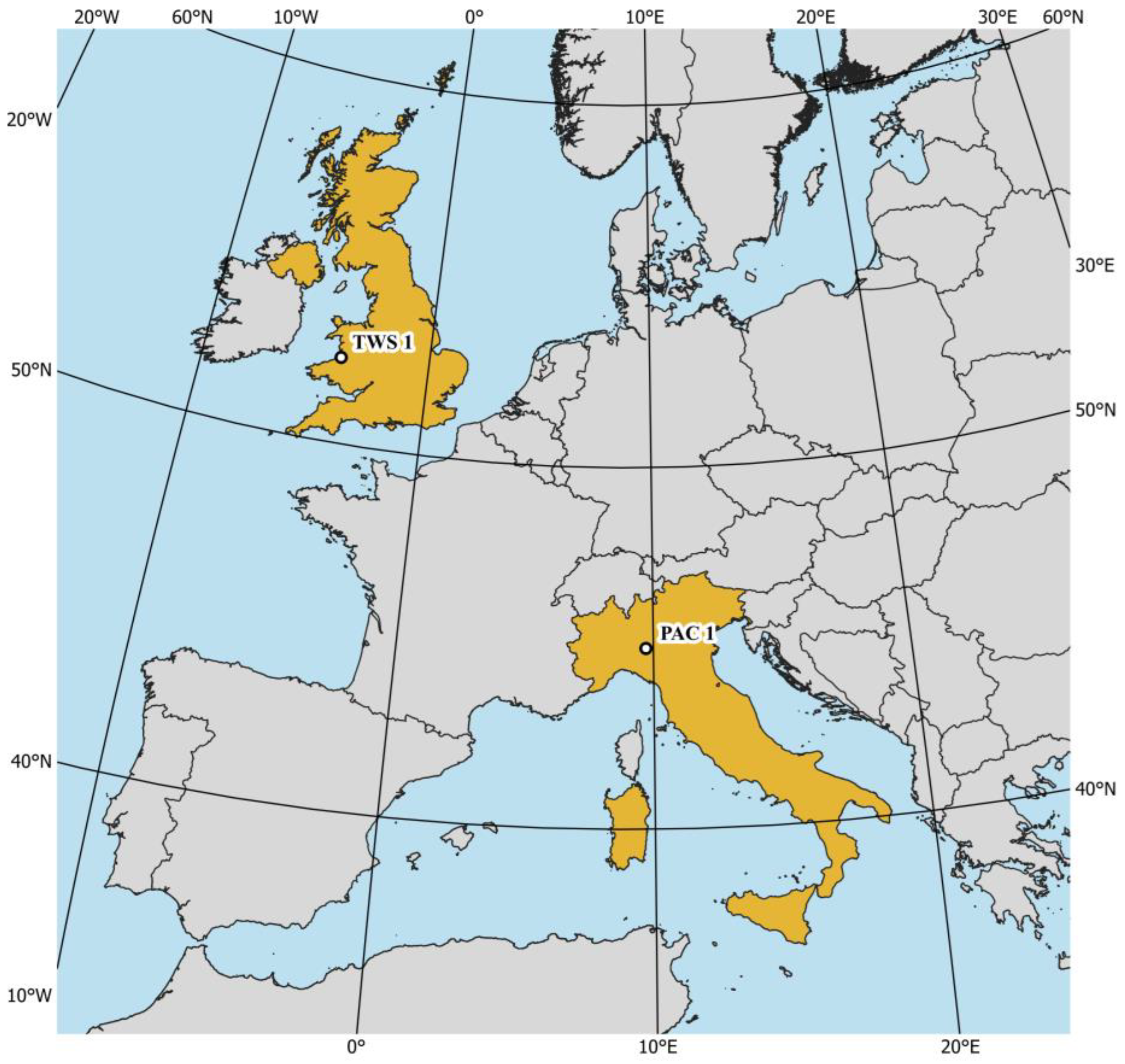
Figure 1. Field experiment locations: PAC 1 is situated in Piacenza (North-West Italy) and TWS in Aberystwyth (Mid-West Wales).
Remotesensing 14 02927 g001
Figure 2. Linear regressions of each VI simulated by the PROSAIL model, between the two sensors (MicaSense and SlantRange). The color code represents the point count distribution scaled to maximum of 1 in each hexagon. The blue dashed line represents the 1:1 relationship and the black line represents the linear regression.
Remotesensing 14 02927 g002
Figure 3. Importance of the RF models variables for crop trait estimations and for yield prediction, expressed as the drop-out loss of model performance (RMSE) for each variable related to the drop-out loss of the full model (dotted line). * The RMSE values are in (%), (cm), (Mg DM ha−1), (Mg DM ha−1), and (Mg DM ha−1), respectively, for the light interception, plant height, green leaf biomass, standing biomass, and yield.
Remotesensing 14 02927 g003
Figure 4. Frequency distribution of Miscanthus traits at the two locations in PAC 1 and TWS 1: (a) light interception (%), (b) plant height (cm), (c) green leaf biomass (Mg DM ha−1), and (d) standing biomass (Mg DM ha−1).
Remotesensing 14 02927 g004
Figure 5. Estimated vs. measured crop traits on the ground of four Miscanthus hybrids’ growth at PAC 1 and TWS 1: (a) light interception (%), (b) plant height (cm), (c) green leaf biomass (Mg DM ha−1), and (d) standing biomass (Mg DM ha−1). The blue dashed line represents the 1:1 relationship and the black line represents the linear regression.
Remotesensing 14 02927 g005
Figure 6. NRMSE values of the RF models obtained for each crop trait assessed in four hybrids grown at the two locations in PAC 1 and TWS 1. Note: lower values indicate higher estimation accuracies.
Remotesensing 14 02927 g006
Figure 7. Frequency distribution of yield (Mg DM ha−1) for the different Miscanthus hybrids at the two locations, PAC 1 and TWS 1.
Remotesensing 14 02927 g007
Figure 8. The (a) predicted vs. measured yield (Mg DM ha−1), (b) NRMSE of the RF model for yield prediction, and (c) boxplot of the modified days of the year (DOYM) of the peak derived from the complete time series of the 5 VIs (greenWDRVI, GNDVI, MTVI2, NDVI, and WDRVI,) of different Miscanthus hybrids, at two locations, PAC 1 and TWS 1.
Remotesensing 14 02927 g008
Figure 9. (a) Time series of the five VIs (GNDVI, greenWDRVI, MTVI2, NDVI, and WDRVI) fitted via the generalized additive model (GAM) throughout the growing season of Miscanthus in PAC 1. Modified days of the year (DOYM) were calculated by adding 365 to the DOY of the corresponding year from January on. (b) Variation of the peak of the VIs derived from the complete time series of the VIs as compared to the peak of the VIs derived from the partial time series of the VIs. The DOYM of the UAV flights performed during the season in PAC 1 are reported in the x-axis. In the y-axis, the peak differences between the peak derived to the end of the season in PAC 1 (397 DOYM) and the peak derived from partial time series fitted until the DOYM of the UAV flight, are reported.
Remotesensing 14 02927 g009
Figure 10. (a) Time series of the five VIs (GNDVI, greenWDRVI, MTVI2, NDVI, and WDRVI) fitted via the generalized additive model (GAM) throughout the growing season of Miscanthus in TWS 1. Modified days of the year (DOYM) were calculated by adding 365 to the DOY of the corresponding year from January on. (b) Variation of the peak of the VIs derived from the complete time series of the VIs as compared to the peak of the VIs derived from the partial time series of the VIs. In the x-axis, the DOYM of the UAV flights performed during the season in TWS 1 are reported. In the y-axis, the peak differences between the peak derived to the end of the season in TWS 1 (421 DOYM) and the peak derived from partial time series fitted until the DOYM of the UAV flight are reported.
Remotesensing 14 02927 g010
Figure 11. NRMSE values of the RF model for yield prediction trained with the peak of the VIs, derived from the complete time series and tested with the peak of the VIs derived from the partial time series fitted until the modified days of the year (DOYM) of the UAV flight, at the two locations PAC 1 and TWS 1.
Remotesensing 14 02927 g011
Table 1. Unmanned aerial vehicles (UAVs) and multispectral cameras used to perform flights in the two locations, with their respective characteristics of spectral bands, central wavelength, and full width at half maximum (FWHM).
LocationUAVMultispectral Camera Characteristics
ModelBandCentre (nm)FWHM (nm)
PAC 1DJI M210 RTKMicaSense RedEdge-MxBlue47532
Green56027
Red66814
Red edge71712
Near-infrared84057
TWS 1DJI M210SlantRange 4PBlue470100
Green550100
Red65040
Red edge71020
Near-infrared850100
Table 2. List of the vegetation indices evaluated in random forest models for crop traits estimation and yield prediction of Miscanthus.
VIsEquationReference
Datt1 NIR RedEdge NIR + Red [66]
EVI2 2.4 NIR Red 1 + NIR + Red [67]
GNDVI NIR Green NIR + Green [68]
GOSAVI NIR Green NIR + Green   + 0.16 [69]
greenWDRVI 0.1 NIR Green 0.1 NIR + Green + 1 0.1 1 + 0.1 [70]
MSAVI 2 NIR   + 1 ( 2 NIR   + 1 ) 2 8 ( NIR     Red ) 2 [71]
MTVI1 1.2 ( 1.2   ( NIR Green ) 2.5 ( Red Green ) ) [72]
MTVI2 1.5 1.2 ( NIR     Green ) 2.5 ( Red     Green ) ( 2 NIR   + 1 ) 2 6 NIR   5 Red 0.5     [72]
NDRE NIR RedEdge NIR + RedEdge [73]
NDVI NIR Red NIR + Red [74]
OSAVI ( 1 + 0.16 ) NIR Red NIR + Red   + 0.16 [75]
OSAVI2 ( 1 + 0.16 ) NIR RedEdge NIR + RedEdge   + 0.16 [76]
rededgeWDRVI 0.1 NIR RedEdge 0.1 NIR + RedEdge + 1 0.1 1 + 0.1 [70]
SAVI ( 1 + 0.5 ) NIR Red NIR + Red   + 0.5 [77]
WDRVI 0.1 NIR Red 0.1 NIR + Red + 1 0.1 1 + 0.1 [70]
Table 3. Ranges of input parameters for the PROSAIL model for the generation of the LUT.
ParameterAbbreviationUnitValues (Step)
LeafStructure parameterNUnitless1–2 (1)
Chlorophyll contentLCCµg cm−210–80 (10)
Relative equivalent water thicknessCwr%20–80 (20)
Dry matter contentCmg cm−20.01–0.025 (0.005)
CanopyLeaf area indexLAIm2 m−21–8 (1)
Leaf inclination distributionLIDF Spherical
Hotspot parameterhotm m−10.05–0.45 (0.2)
Solar zenith anglettsdeg20–80 (10)
Observer zenith anglettodeg5–10 (5)
Relative azimuth anglepsideg180–220 (10)
Structure parameterNUnitless1–2 (1)
Publisher’s Note: MDPI stays neutral with regard to jurisdictional claims in published maps and institutional affiliations.

