
Design and Demonstration of a Novel Long-Range Photon-Counting 3D Imaging LiDAR with 32 × 32 Transceivers
by
 , , and
Changsheng Tan
1,2 ,
,
Wei Kong
1,2,3,*,
Genghua Huang
1,2,3,
Jia Hou
1,
Shaolei Jia
1,
Tao Chen
1,2,3 and
Rong Shu
1,2,3 1
Key Laboratory of Space Active Opto-Electronics Technology, Shanghai Institute of Technical Physics, Chinese Academy of Sciences, Shanghai 200083, China
2
University of Chinese Academy of Sciences, Beijing 100049, China
3
Shanghai Research Center for Quantum Sciences, Shanghai 201315, China
*
Author to whom correspondence should be addressed.
Remote Sens. 2022, 14(12), 2851; https://doi.org/10.3390/rs14122851
Submission received: 6 April 2022
/
Revised: 12 June 2022
/
Accepted: 13 June 2022
/
Published: 14 June 2022
(This article belongs to the Section Engineering Remote Sensing)
Abstract
:Geiger-mode single-photon LiDAR is an important tool for long-distance three-dimensional remote sensing. A planar-array-based photon counting LiDAR that uses 32-by-32 fiber arrays coupled to an optical lens as a transceiver unit was developed. Using transmitters and receivers with the same design, the proposed device easily achieves a high-precision alignment of 1024 pixels and flexible detection field-of-view design. The LiDAR uses a set of relay lenses to couple echoes from the receiving fiber arrays to the pixels of a planar-array single-photon detector, which has a resolution enhanced by a factor of four (64-by-64) relative to the fiber array to reduce cross talk from neighboring pixels. The results of field experiments demonstrate that the proposed LiDAR can reconstruct a three-dimensional image from a distance of 1600 m. Even at an acquisition time of only 40 ms, targets with an area of approximately 50% can still be identified from 200 frames. These results demonstrate the potential of the LiDAR prototype for use in instantaneous high-density point-array measurement and long-range wide-FoV 3D imaging, which can be used in remote sensing applications such as airborne surveys and mapping. In the future, we will integrate the proposed LiDAR prototype and the pose measurement system to take the aircraft-based 3D imaging remote sensing experiments.
1. Introduction
Light detection and ranging (LiDAR) is widely used as an active photoelectric detection method with excellent directivity and high range precision in remote sensing scenes such as airborne mapping [1], urban surveys [2], autonomous vehicles [3], and spatial navigation [4]. As they allow the scattering echo to be attenuated to the order of single photon by increasing the operating range, high-sensitivity single-photon avalanche photodiode (SPAD) detectors are being increasingly adopted for receiving, thus promoting the rapid application of photon-counting LiDAR [5]. Such systems can achieve high-sensitivity measurement with limited laser energy, particularly in long-range scenes, and have contributed significantly to the field of three-dimensional (3D) imaging in the past few decades [6]. Current photon-counting 3D imaging LiDAR is primarily achieved through the use of individual detectors in conjunction with high-precision mechanical scanning [7,8]. In such a configuration, high-precision 3D imaging is achieved by steering a pulse beam in a pointwise manner along a specific angle across a target scene via a scanning unit and then using a single high-sensitivity SPAD detector to detect echo photons reflected from the target.
The combined advantages of a simple structure and high transceiver efficiency make scanning pulsed LiDAR suitable for outdoor imaging applications [9]. However, limitations in the scanning speeds of mechanical scanning systems make it difficult to achieve high-density 3D imaging at high frame rates with a single beam. Some researchers have attempted to solve this problem by developing faster scanning devices (e.g., MEMS scanning mirrors or optical phased arrays) to reduce the acquisition time [10,11], increasing the number of scanned beams to improve the detection coverage area [12,13], or adaptively determining the residence time of each depth acquisition [14].
The recent maturation of large-scale single-photon focal plane array detector technology has made it possible for LiDAR devices to acquire 3D images in the manner of an image sensor [15,16,17]. Unlike scanning pulsed LiDAR, planar-array-based LiDAR do not require mechanical moving components, and they employ detector arrays instead of a single detector to receive echo photons. This allows the LiDAR to obtain a 3D image of a target within its coverage area using a single-exposure process. Such mechanism has significant advantages relative to scanning LiDAR in terms of acquisition speed and pointing accuracy, making it an area of active research. Several research institutions have conducted 3D imaging demonstrations based on SPAD array detectors. Albota et al. conducted active 3D imaging experiments based on a 4 × 4 GmAPD module and a microchip laser source [18]. Hiskett et al. proposed a long-range non-scanning 3D imaging system based on an InGaAs/InP 32 × 32 Gm-APD array camera [19]. Henriksson et al. reported a panoramic LiDAR based on a SPAD array and successfully acquired panoramic depth images of outdoor forest targets within 1 km at night [20]. This detection technology, which is similar to the global shutters used in imaging sensors, is well suited to the detection of objects with relative motion.
To achieve non-scanning flash 3D imaging, most planar-array-based single-photon LiDARs employ a SPAD array that is directly placed on the focal plane of the receiving telescope and use a laser source with a large divergence angle to cover the entire receiving field-of-view (FoV) [4,21,22]. Given the detector’s limited fill factor, however, this approach wastes most of the laser energy. This problem can be resolved by using optics to split the laser beam into multiple beams corresponding to the respective FoVs of the receiving pixels. For example, the Sigma Space Corporation used diffractive optical elements (DOEs) to split a 532-nm beam into a 10-by-10 array to achieve 100-beam area array 3D imaging [23,24,25]. In addition, Lee et al. proposed a 7-beam lidar by splitting the beam with two hexagonal prisms [26]. Yu et al. reported an airborne lidar surface topography simulator (ALSTS) instrument with a 16-beam push-broom configuration. The output laser is separated into a 4 × 4 grid pattern of spots in the far field by a pair of microlens arrays at the transmitter [27]. However, to date, no LiDAR system capable of splitting a laser beam into more than one thousand beams has been published, but such capabilities are still the pursuit of LiDAR instrument conceptual design. For example, the Lidar Surface Topography (LIST) mission proposed by NASA’s Earth Science Technology Office (ESTO) planned to launch 1000 beams from a 400 km Earth orbit with beam separation of 5 m at earth surface, which is far more than the 6-beam configuration of ATLAS lidar aboard on an ICESat-2 satellite [28].
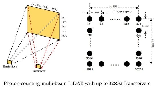
In this work, a novel transceiver structure for multi-beam photon-counting lidar was proposed to make the three-dimensional imaging. In order to achieve high-precision beam pointing accuracy, the proposed system utilizes a microlens array to couple its laser energy into a 32-by-32 fiber array to achieve beam separating at a scale of over 1000. Using a carefully designed transmitter and receiver optical structure, the LiDAR achieves low-cross talk 3D imaging with a resolution of 32 by 32 via a SPAD array. This paper describes the system structure and data processing method applied by the proposed LiDAR in Section 2, and then presents and analyzes the results of the daytime field experiment in detail in Section 3. In Section 4, we discuss the advantages of the proposed lidar structure, summarize the performance, and present an outlook for the future work.
2. Instrument Description
2.1. Transceiver Optics
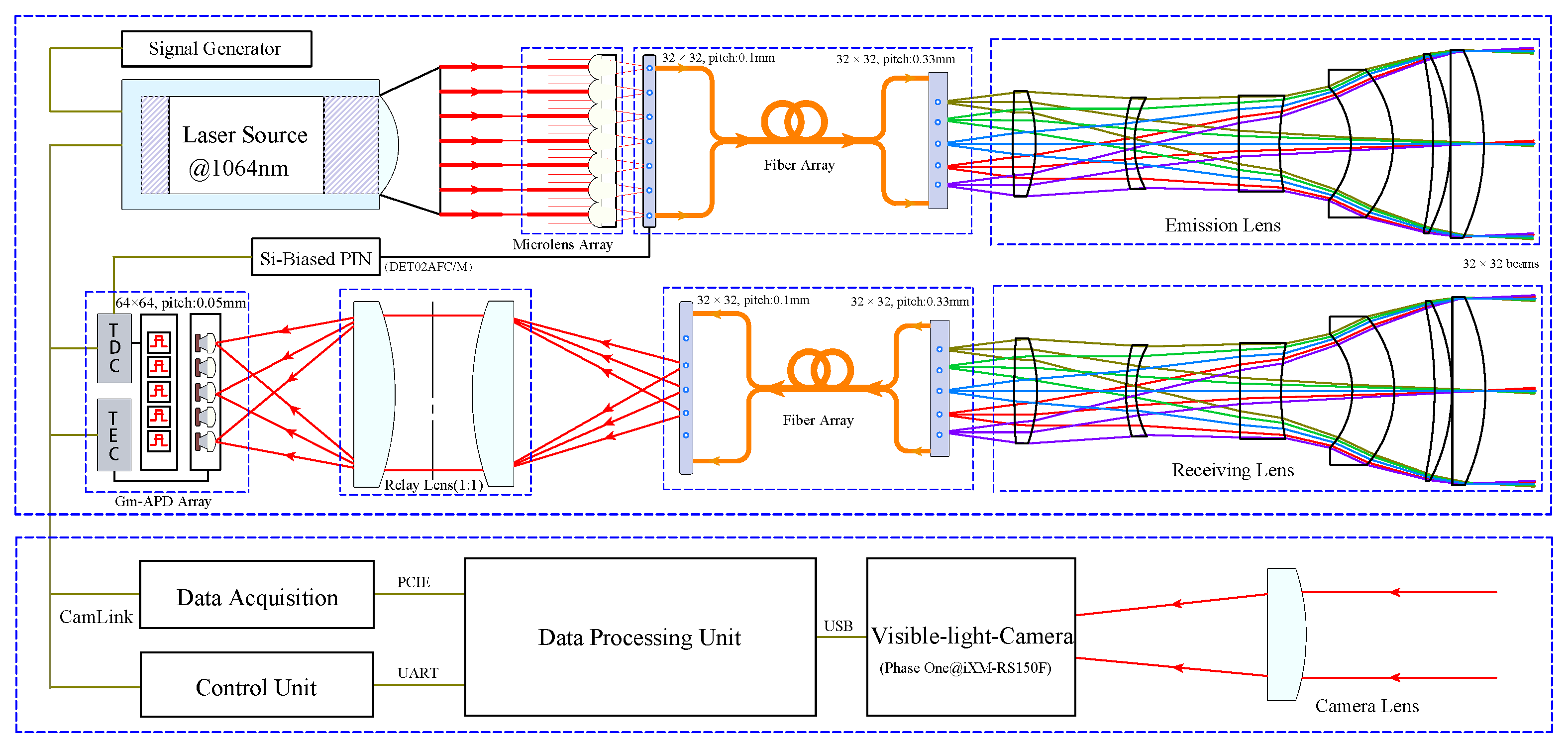
Figure 1 shows a schematic of the system, which comprises a transmitter, receiver, and visible-light camera. The LiDAR transceiver uses an off-axis design to reduce the interference of atmospheric backscattering from near range. At the transmitter, a near-infrared pulsed laser emits pulsed light at 1064 nm with a rated output power of 0.62 W. Instead of active Q-switching, the laser adopts a passively Q-switched scheme to avoid the electromagnetic interference (EMI) form the high-voltage switch circuit. A pulse duration of approximately 1 ns makes the echo photons more concentrated, reducing the ranging errors. The collimated beam produced by the laser is then divided and coupled by a 2D microlens array into a 32-by-32 fiber array. The microlens and fiber array port at the coupling end have the same space pitch of 0.1 mm and their relative positioning is finely adjusted to maximize the coupling efficiency. Although the transmitting fiber array for laser energy transformation has the same 32-by-32 resolution at each end, its space pitch changes from 0.1 mm at the coupling end to 0.33 mm at the collimating end. A lens with a telecentric optical design is used to collimate the laser beam into multiple beams, each having an energy of approximately 0.12 J and a single-beam divergence of 300 rad. The 1024 beams are angularly separated at a pitch of 1.97 mrad, allowing the total FoV of the LiDAR to reach 3.5. The main parameters of the constructed system are shown in Table 1.
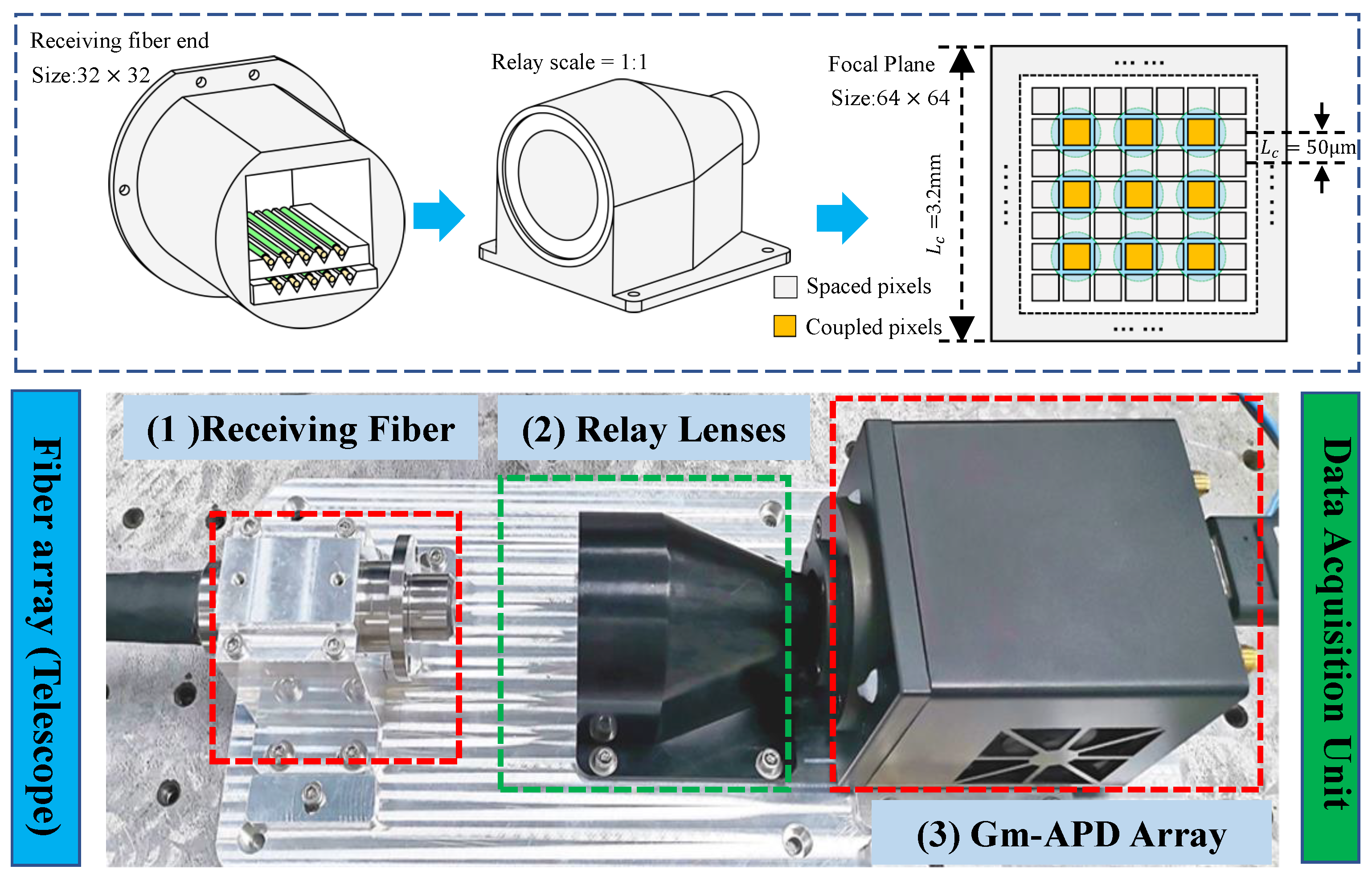
In the receiver, target echoes are filtered by an ultra-narrow bandpass filter with a bandwidth of 0.5 nm and collected by another telecentric optical lens. The receiving lens has a focal length of 166 mm and an effective aperture of 34 mm. It gathers the echoes and couples them into a receiving fiber array with a 32-by-32-resolution and a core diameter of 50 m. As shown in Figure 1, the receiving and transmitter optics have nearly the same design. The receiving fiber array’s space pitch changes from 0.33 mm at the receiving lens port to 0.1 mm at the SPAD detector port. Figure 2 shows the structure used to couple the signal from the receiver fiber array to the SPAD detector. The SPAD detector has a 64-by-64 resolution, which is four times larger than that of the fiber array, and a pixel pitch of 50 m. A set of relay imaging lens with magnification of 1:1 images the fiber end face into the detector. Because only a quarter of the pixels of the SPAD detector are illuminated under this configuration, a redundant design that can reduce the crosstalk effect between the adjacent pixels of the SPAD detector is achieved.
The fiber array-based optical design of the LiDAR transceiver has several advantages. First, its field of view can be flexibly designed by changing the focal lengths of the transmitter and receiver simultaneously. Second, the fiber array-based design enables multi-beam alignment between the transmitter and receiver. By sending light with the same wavelength as that of the laser back through the receiver fiber array, far-field spot images of the transmitter and receiver can be observed together on the planar imaging sensor of the parallel light pipe and then adjusted until they coincide to ensure alignment between the LiDAR transmitter and receiver. Finally, the structure can be easily adapted to different detectors by changing the structure of the fiber array at the receiver.
As shown in Figure 2, the InGaAs/InP based SPAD detector has a highly integrated structure. It has a high photon detection efficiency of approximately 15% at near-infrared wavelengths. The detector can operate in Geiger mode by setting the reverse-bias voltage to exceed its breakdown voltage. In this configuration, echo photons illuminating onto the photosensitive area of the detector are multiplied into electrical pulses via the avalanche effect, which are then converted into distance information by the time-to-digit converter (TDC) circuits embedded in the detector. This distance information is then transferred to the computer via a camera link cable. The detector operates in external trigger mode and has a resolution of 1 ns and maximum gate width of 4 s, which correspond to a distance measurement range of 600 m. To image targets at long distances, the detector can delay triggering of the TDC circuits for a programable time interval.
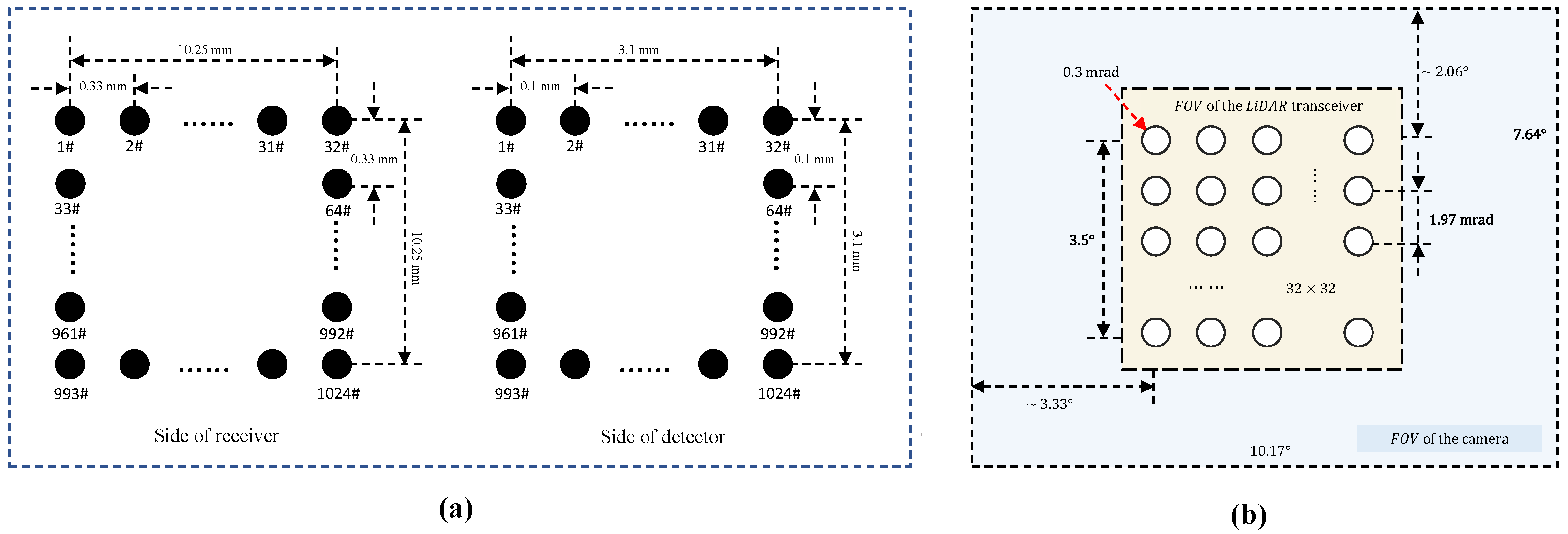
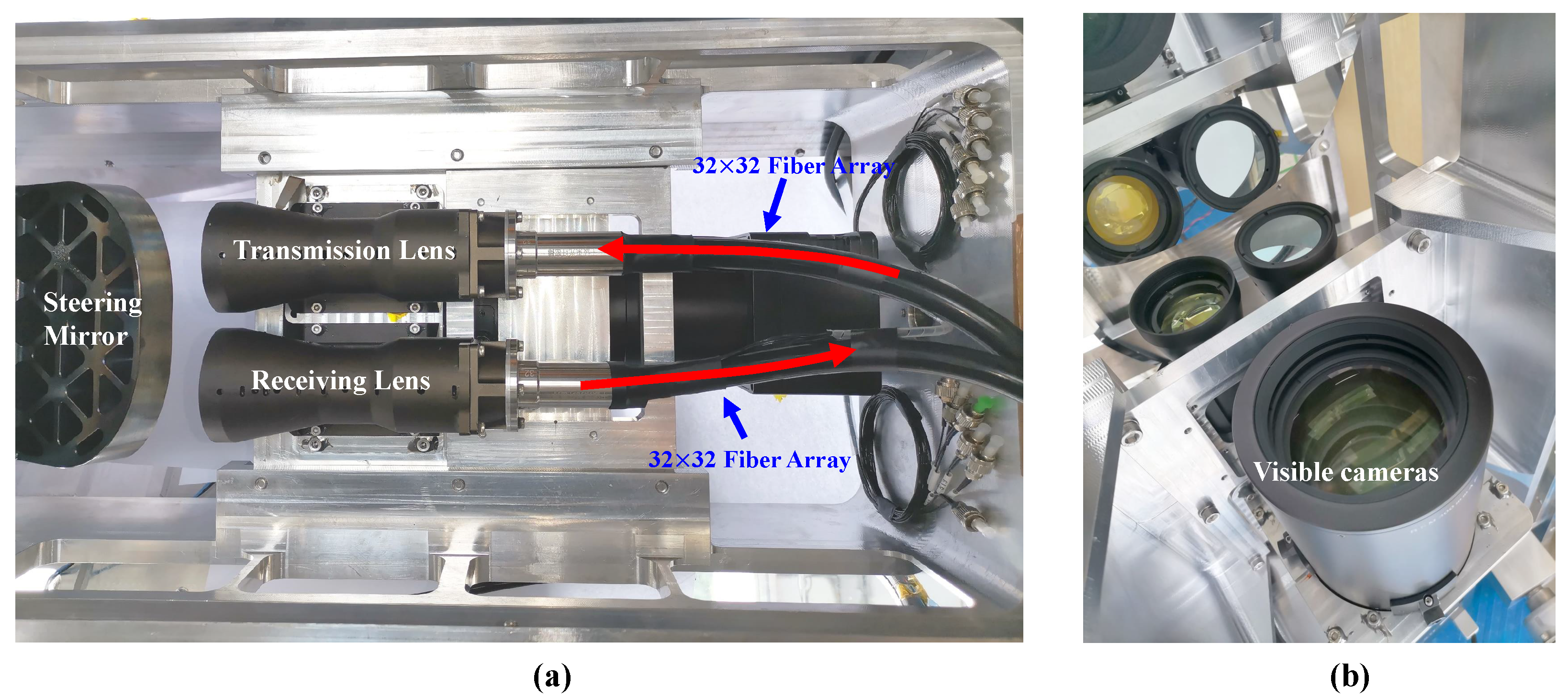
To calibrate the detection FoV and enable the fusing of visible images, a visible camera with a resolution of 14,204 by 10,652 and a geometric size of 53.4 mm by 40.0 mm is installed in the system. The visible camera has a low-distortion lens with a focal length of 300 mm. Its field of view is 10.17 degrees by 7.64 degrees, and it is aligned along the same viewing direction as that of the LiDAR transceiver. Figure 3a shows the arrangement of the coupling faces of the receiving fiber array, which determines the relative position of the beams. Figure 3b shows a schematic of the FoV relationship between the LiDAR and visible camera; the relative positioning between the pixels of the visible camera and the laser beams has been calibrated in a laboratory. Figure 4a,b show physical views of the system’s transmitting and receiving optics and the visible camera. The three components are integrated within an aviation aluminum alloy frame. A large mirror mounted on the assembly is used to steer the observation direction.
2.2. Data Processing Method
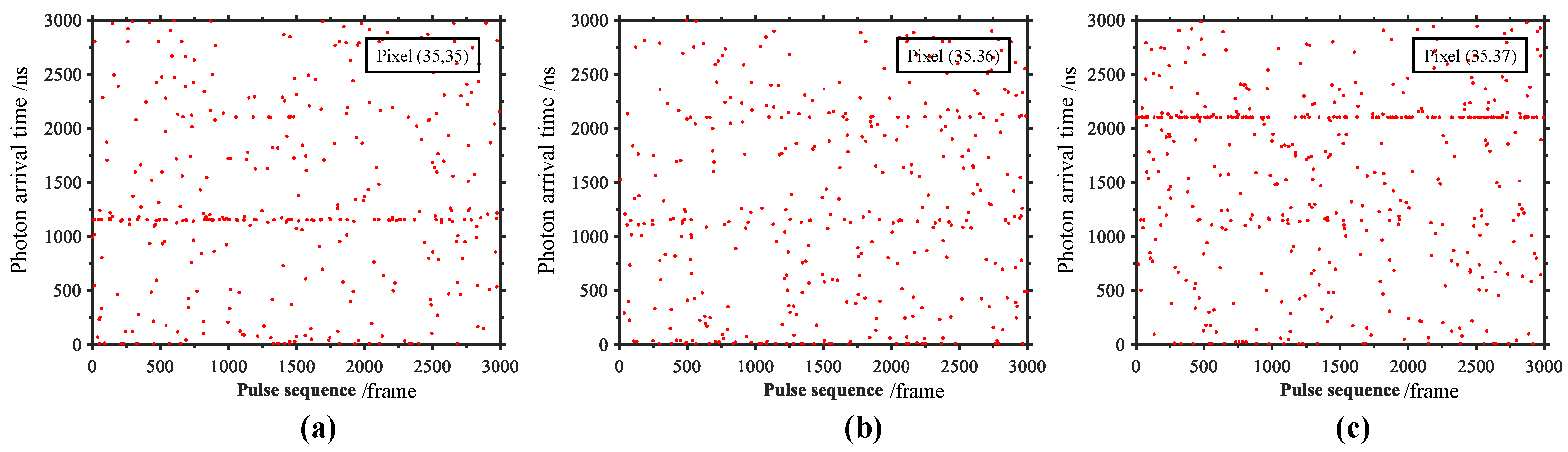
Figure 5 shows a typical signal received at three adjacent pixels of the SPAD detector. Pixels (35, 35) and (35, 37) of the SPAD detector correspond to pixels (18, 18) and (18, 19) of the LiDAR transceiver. Each red dot represents a photon event plotted in terms of its pulse sequence (horizontal axis) and time difference relative to the gate opening time (vertical axis). The original photon events corresponding to the dark count and daytime solar background primarily originate from noise. Additionally, the crosstalk within the SPAD detector is indicated by pixel (35, 36), which has no fiber coupling and vaguely displays the target signals of the neighboring pixels (35, 35) and (35, 37) at approximately 1200 and 2100 ns. The redundant design in which only one-quarter of the pixels are used for signal acquisition can reduce the crosstalk between adjacent pixels within the LiDAR transceiver. The adjacent beams represented in Figure 5a,c clearly have no interference with each other. Although there is approximately 20% crosstalk between adjacent pixels in the SPAD detector, the redundant design reduces the crosstalk within the overall LiDAR transceiver significantly.
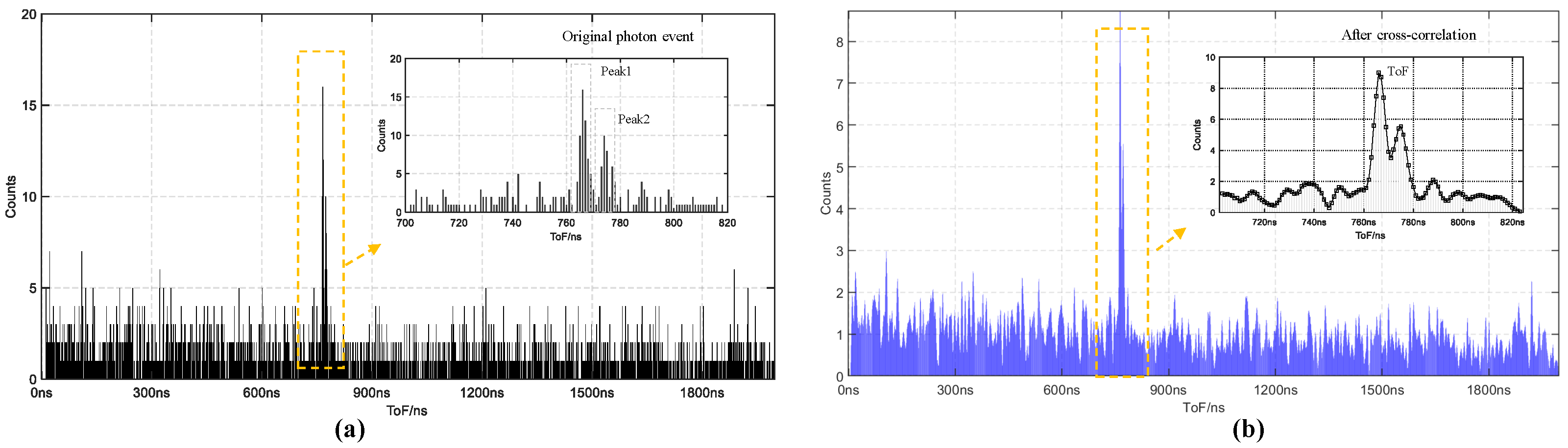
At high signal-to-noise ratio conditions such as those occurring during nighttime, a target position can be accurately reconstructed by accumulating photon events that are recorded at multiple frames of pulses. However, if this approach is applied to outdoor imaging scenarios, especially those occurring during daytime conditions, more of the photons that trigger the SPAD detector will originate from the solar background noise than from the target scattering signal. To meet the requirements for detection under strong background noise conditions at long distances, the system adopts a cross-correlation strategy to recover depth from the photon data.
Figure 6 shows the flow of the algorithm that is applied to the individual beams. First, is defined as the original histogram sequence generated from the recorded photons, as shown in Figure 6a. For signals with strong background noise counts, the signal-to-noise-ratio of this sequence will be poor for depth extraction. A cross-correlation between and the normalized Gaussian kernel function, , which is obtained by measuring the instrumental response function in the laboratory, is then taken. The reconstruction strategy can be written as , where F represents fast Fourier transform; this process is given in the following convolutional form in the discrete-time domain [29]:
Application of Equation (1) smooths the histogram sequence. By searching for maximum value locations in the smoothed histogram, the depth information for a single beam can be extracted [30]. For some beams that do not irradiate onto the target or for which the signal-to-noise ratio is extremely poor, mis-extraction can also happen, but the rarely mis-extracted depth points in the 3D image can be quickly removed by voxel filtering [31,32].
3. Field Experiments and Discussion
3.1. Case 1 at 500 m
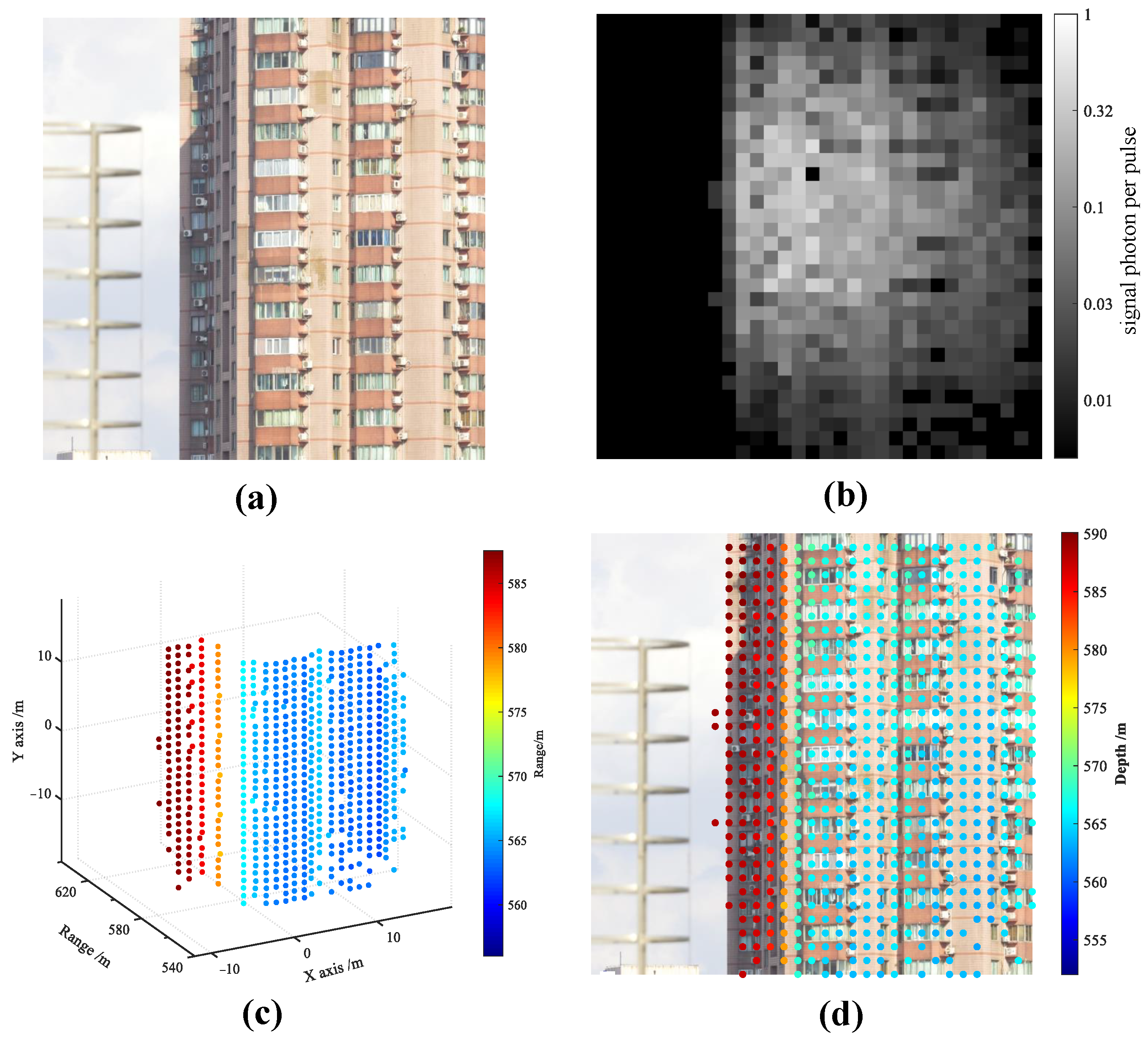
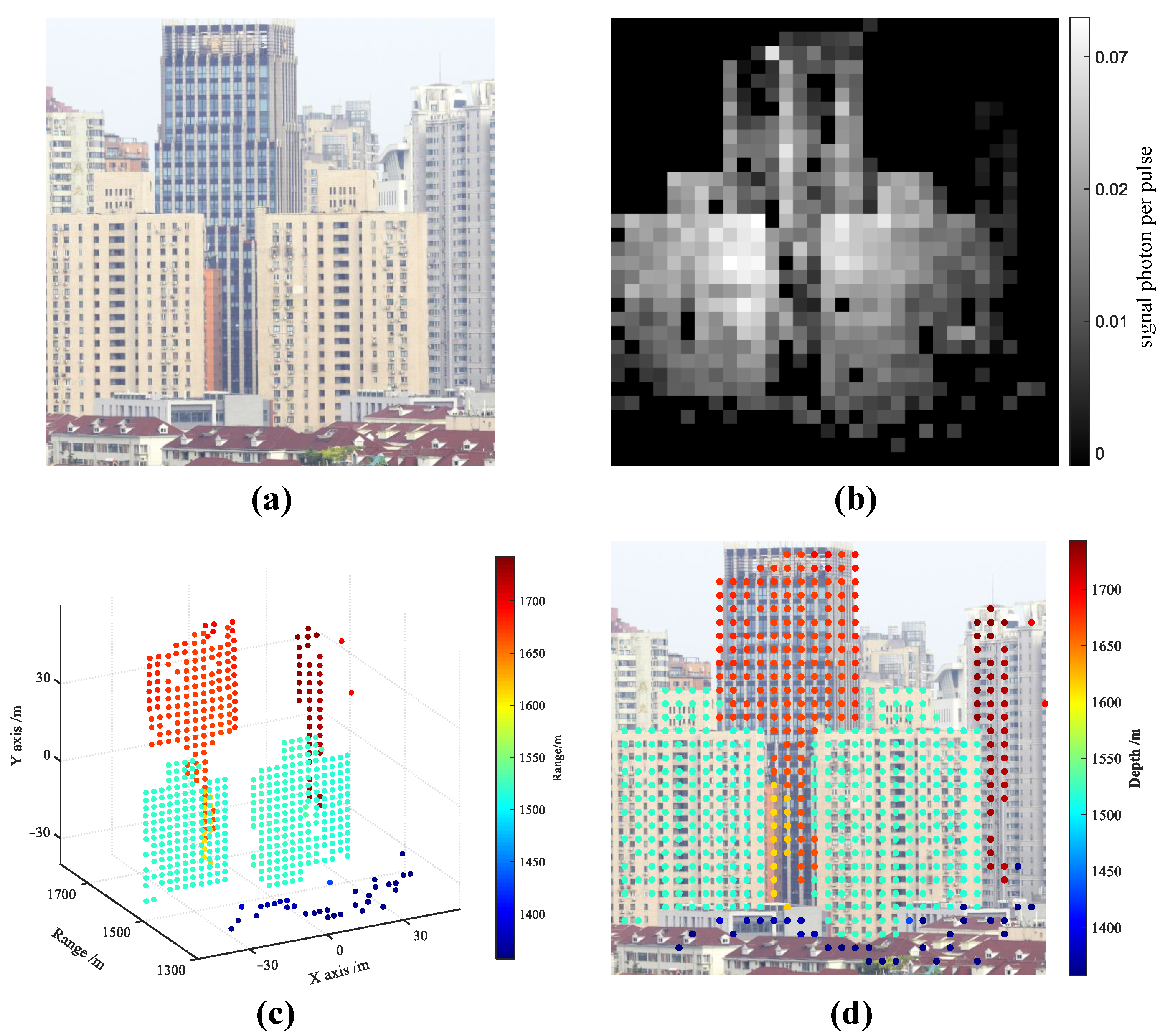
To verify the 3D imaging performance and anti-interference ability of the proposed system under the condition of strong background noise, we conducted field experiments in which the LiDAR was aimed at a target 500 m away on a sunny day in which the atmospheric visibility was 15 km. Under this condition, the atmospheric extinction coefficient at the near surface was approximately 0.13 km and the dual-way transmittance at 500 m was 88%. In the experiment, the detector timing delay was set to 3 s to make the effective detection range cover the entire target building; to achieve this, the detector strobe gate width was set to 2 s with a maximum detection range of 300 m. Figure 7 shows the visible image, gray image recovered from the LiDAR data, 3D distribution of the retrieved depth data at all LiDAR pixels, and the fusion data incorporating the visible image and LiDAR results. The results were recovered from 5000 frames of data. The 3D data shown in Figure 7d are consistent with the building’s structure lines.
The limitations of the data processing capability of a TDC chip mean that a SPAD detector with 4096 pixels can only record one photon event per acquisition cycle. Therefore, a noise photon event from the solar background occurring prior to a signal photon event can hide the signal photon and make it unrecognizable. Despite the use of an ultra-narrow-bandpass filter to suppress the solar background, the noise photons occurring at daytime can have a significant impact on LiDAR detection. In this case, the average photon occurrence will be 49.26% per pulse, but only 13.6% of the total photons will be recognized as signals. If the target is close to the center of the strobe gate, the solar background noises will further reduce the probability of detecting signal photons by approximately 25%. It is therefore beneficial to increase the detection probability of this system by opening the range gate as close as possible to the target.
Figure 7b shows the distributions of signal photon number by pulse over the LiDAR’s FoV. As the distances between the imaging system and different parts of the building do not vary significantly, the intensities within the grayscale image can reflect the energy distribution of the transmitting fiber array. Given the non-flat-top distribution characteristics of the laser spot, the echo signal intensities in the central area will be stronger than at the image edge. The probability of photons reaching the detector and producing primary photoelectrons can be described approximately as a Poisson distribution [33]. If the signal photon arrival time is given by and the minimum time resolution interval by , where , the probability of a photon being detected at instant is equal to the product of the probability of not being triggered before and the probability of being triggered at , which can be expressed as [34]:
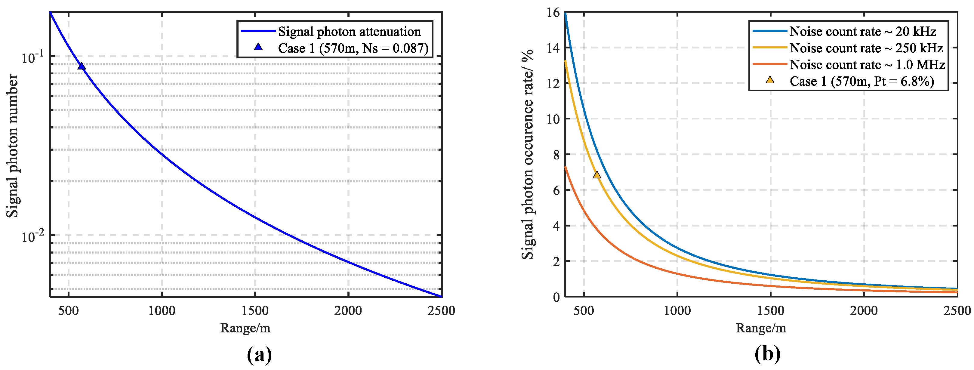
where is the average signal counting rate and the average noise counting rate can be calculated by measuring received non-emitted pixels. During the experiment, the probability of noise photon triggering within each interval was extremely low (approximately 0.0238%); therefore, photons in the ns range caused by jitter errors were considered to be signal photon counts falling within . The average trigger probability per pixel within the signal interval was 6.8%. Photons that trigger the avalanche effect in a detector are called primary photons. Using Equation (2), the average primary signal photon count per pulse was calculated to be 0.087 based on the lapse of 800 ns between the target and the selective strobe gate. Based on these results, the detection capability of the system could be evaluated quantitatively according to the LiDAR ranging equation [5]. Assuming that the operating distance is R, the average number of signal photons that each beam can receive is
where h is the Planck constant, c denotes the speed of light, is the wavelength, and is the overall efficiency of the optical system, including transmitter, receiver, and detector’s equivalent fill factor. is the detection efficiency, is the reflectivity, and are the received field-of-view and beam divergence angle, respectively, is the atmospheric transmittance, is the effective area of the receiving lens, and is the average emitted energy of each beam. Equation (3) shows that the signal photon number is inversely proportional to the square of the distance while the target reflectivity remains unchanged.
Based on the estimated signal photon number per pulse in case one, 0.087, the signal photon number at different distances is presented in Figure 8a. In the presence of solar background noises, the signal occurrence probabilities that are calculated from Equation (2) are shown in Figure 8b. The three different noise intensities with noise photon count rate of 20 kHz, 250 kHz, and 1 MHz correspond to the dark count rate of the detector, the solar background noise level of case 1, and the condition when the sun shines almost directly on the receiving system. Obviously, strong ambient noise will degrade the signal detection probability. For case 1, the signal detection probability is approximately 17% less than the solar background noise free condition when only the detector dark counts are present. If the solar background noise count rate is as strong as 1 MHz, the signal detection probability per pulse will drop from 6.8% in case 1 to only 3.82%. Benefitting from the narrow bandwidth filter that is inserted in the LiDAR receiver, the influence from the solar background noises can be maintained at an acceptable level.
On the other hand, the echo signal will become extremely strong if the target is close enough, which is better for signal extraction. However, at this condition, several signal photons arrive at a single pixel simultaneously, the detector will only resolve the first event. Then, distance bias will occur. Although we use short-pulse laser with pulse duration of less than 1 ns to reduce this effect, the distance deviation can still become quite large when the signal is extremely strong. In these special conditions, a neutral density filter will be placed at the receiving aperture to attenuate the signal intensity. Certainly, in most situations, this effect is so weak for the system that no neutral density filter is required.
3.2. Case 2 at 1600 m
To verify the LiDAR performance at longer range, another field experiment was carried out using a set of targets at distances in the range of approximately 1600 m. The detector’s opening time was set to 9 s after laser firing. In this case, the gate width of the detector was set to 4 s to accommodate targets distributed over a relatively large range of distances. In addition, 5000 frames of data were used for 3D image reconstruction.
As shown in Figure 9, multiple buildings at distances ranging from 1300 to 1700 m are all recognized in the LiDAR data, and the visible-image and LiDAR data within the LiDAR’s field of view agree closely. As seen in Figure 9b, the more distant buildings scattered fewer echo photons than the closer buildings. Most of the beams can be successfully received and registered into the corresponding pixels of the Gm-APD focal plane array.
3.3. Performance at Short Acquisition Time
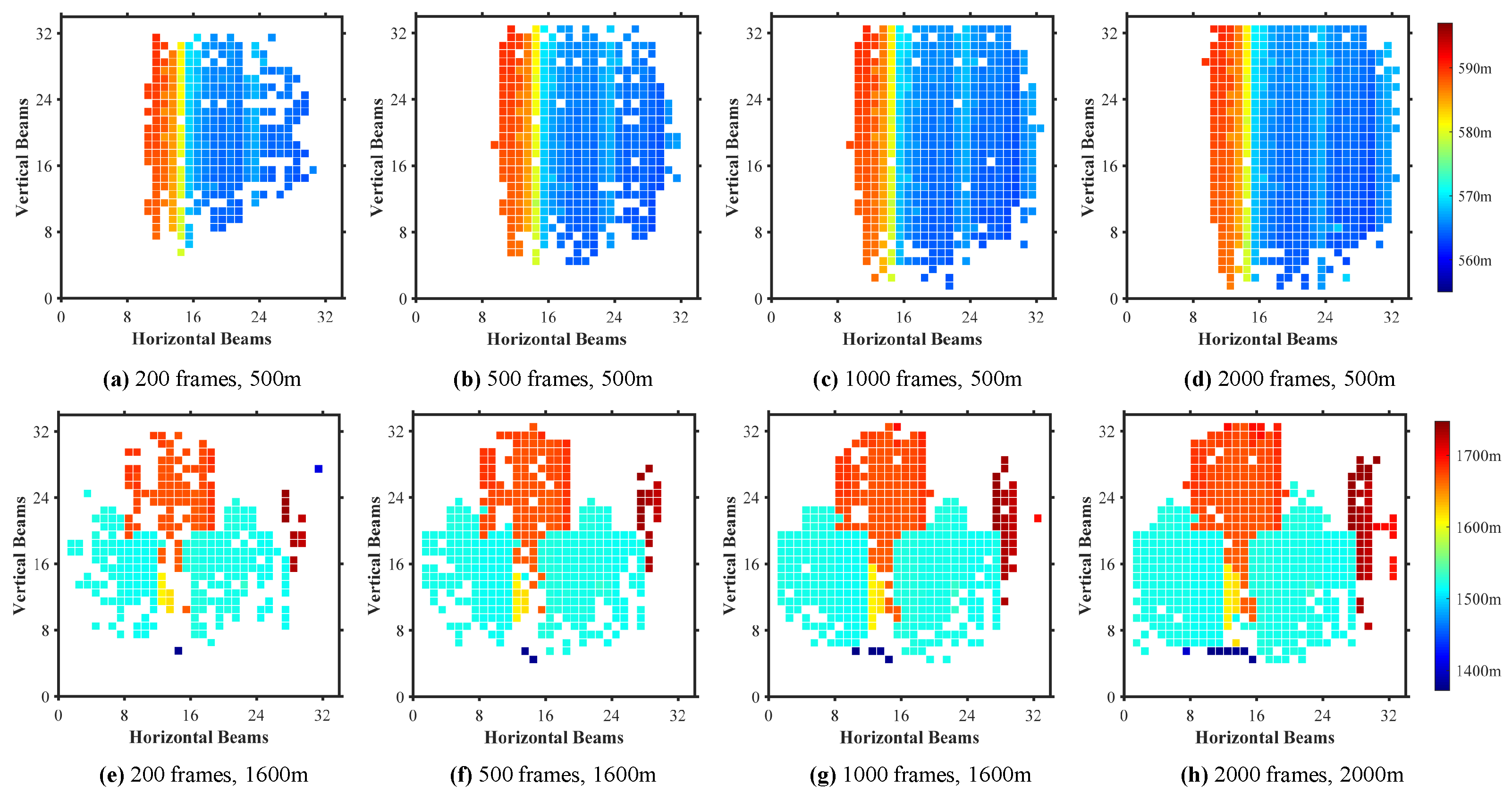
To evaluate the LiDAR performance with fewer frames, depth information for images obtained over 200, 500, 1000, and 2000 frames, respectively, is shown in Figure 10. Figure 10a–d show the results for case 1; Figure 10e,f show the results for case 2. For both cases, we set reconstruction results obtained from 20,000 frames as the reference depth; if the retrieved depth of the LiDAR pixels were within a time range of ns relative to the reference results, the retrieved results were considered to be effective. Obviously, increasing the number of frames used for depth extraction increased the proportion of effective data. Under the conditions with the lowest numbers of frames, the pixels at the edge of the LiDAR field were more difficult to resolve given the low laser energies at the LiDAR edge field. Increasing the number of frames enabled the correct reconstruction of the 3D image at the edge region. In practical applications, it is necessary to use a laser with a flat-top spot to improve the uniformity of beam splitting.
Table 2 lists the proportion of valid beams in each low-frame case relative to the 20,000 frame reference. Even with only 200 frames, at which the acquisition time was only 40 ms, approximately half of the pixels could still be retrieved effectively. These results indicate that the proposed planar-array-based multi-beam photon-counting LiDAR has the potential to be used for fast 3D imaging in remote sensing applications such as long-range dynamic target observation airborne mapping, etc.
4. Conclusions and Outlook
For the extremely sensitivity of the SPAD, photon-counting lidar has low requirements for the laser pulse energy, thereby enabling simultaneous detection of multiple beams under the limited system power supply. On this basis, we report a novel transceiver design for multi-beam single photon counting lidar. In the transmitter, the pulsed laser is coupled into a fiber array by a microlens array; then, a telecentric lens collimates the laser at the other end of the fiber array to multiple beams with a resolution of 32 by 32. The receiver has the similar structure that couples the lidar return into the fiber array, and then a set of relay lens couples the signal at the other end of the receiving fiber array to a SPAD array. In this paper, the system structure, depth extraction method design, and results of daytime field experiments were presented in detail. As a result of the detector’s single-photon sensitivity, the LiDAR system can acquire kilometer-level 3D images. The results of field experiments at a target distance of 1600 m demonstrated that, even at a short acquisition time of only 40 ms, 50% of the 3D imaging area could be reconstructed, indicating that the LiDAR can be applied in dynamic target measurement.
Compared with the beam splitting scheme of DOE and prisms, the transmitter in our system couples the high-energy laser into the fiber array with a micro-lens array, thereby realizing multi-beam splitting. In this design, the laser does not emit light directly to the target, so the lidar is immune to the laser pointing jitter from the temperature and thermal instability. Under the current manufacturing capabilities, the absolute positioning accuracy of the fiber array can easily reach a few micrometers, so the fiber-array-based transceiver design will have excellent laser pointing stability, which is quite beneficial to improve the positioning accuracy of the lidar. In practice, this design can be easily matched to the image data for data fusion. In addition, for the transmitter and receiver to have nearly the same structure, the observation field of view can be easily reconfigured by replacing the pair of telecentric lenses.
In the proposed system, the fiber array with a resolution of 32 by 32 at the receiver is coupled to the Gm-APD array with a resolution of 64 by 64 with a set of relay lenses. Although three quarters of the SPAD pixels are unused, this coupling scheme significantly reduces the crosstalk between neighboring pixels of the lidar field of view. This redundant design can reduce the influence from the 20% crosstalk between adjacent pixels of the Gm-APD array to improve the ranging accuracy.
In the future, we will integrate the lidar with a high precision pose measurement system to make the aircraft-based 3D imaging, as well as further improve the LiDAR’s optical and algorithm efficiency to increase its 3D imaging speed. If the imaging field of view is fixed and the laser beam pointing is stabilized, we will also consider the DOE to split the laser beam, but the receiving fiber array should be specifically designed according to the fringe field of view distortion of the DOE and the receiving telecentric lens. This will improve the performance at the edge of the field of view. In addition, the spatial correlation characteristics of adjacent beams can potentially be used to reduce the signal photon numbers required for depth extraction, thereby further improving the detection range and 3D imaging speed of the LiDAR.
Author Contributions
Conceptualization, G.H., W.K. and C.T.; Writing—original draft preparation, C.T.; Writing review and editing, W.K.; Experiment, processing, and visualization, C.T.; Optics, J.H.; Mechanics, S.J.; Project leader, G.H., T.C. and R.S. All authors have read and agreed to the published version of the manuscript.
Funding
This research was funded by the following funds: Science and Technology Commission of Shanghai Municipality (2019SHZDZX01); National Natural Science Foundation of China (61805268, 61875219); Innovation Foundation of Shanghai Institute of Technical Physics, and Chinese Academy of Sciences (CX-368).
Data Availability Statement
The data that support the findings of this study are available from the author upon reasonable request.
Conflicts of Interest
The authors declare no conflict of interest.
Abbreviations
The following abbreviations are used in this manuscript:
| FoV | field-of-view |
| LiDAR | light detection and ranging |
| TDC | time-to-digit converter |
| SNR | signal-to-noise ratio |
| DOE | diffractive optical elements |
| SPAD | single-photon avalanche photodiode |
| Gm-APD | Geiger-mode Avalanche Photo Diode |
References
- Lin, Y.C.; Manish, R.; Bullock, D.; Habib, A. Comparative Analysis of Different Mobile LiDAR Mapping Systems for Ditch Line Characterization. Remote Sens. 2021, 13, 2485. [Google Scholar] [CrossRef]
- Kulawiak, M. A Cost-Effective Method for Reconstructing City-Building 3D Models from Sparse Lidar Point Clouds. Remote Sens. 2022, 14, 1278. [Google Scholar] [CrossRef]
- Zhao, X.; Sun, P.; Xu, Z.; Min, H.; Yu, H. Fusion of 3D LIDAR and Camera Data for Object Detection in Autonomous Vehicle Applications. IEEE Sens. J. 2020, 20, 4901–4913. [Google Scholar] [CrossRef] [Green Version]
- Pierrottet, D.F.; Amzajerdian, F.; Meadows, B.L.; Estes, R.; Noe, A.M. Characterization of 3D imaging lidar for hazard avoidance and autonomous landing on the Moon. In Proceedings of the SPIE Conference on Laser Radar Technology and Applications XII, Orlando, FL, USA, 3 May 2007; Volume 655. [Google Scholar] [CrossRef]
- Fouche, D.G. Detection and false-alarm probabilities for laser radars that use Geiger-mode detectors. Appl. Opt. 2003, 42, 5388–5398. [Google Scholar] [CrossRef]
- McManamon, P.F. Review of ladar: A historic, yet emerging, sensor technology with rich phenomenology. Opt. Eng. 2012, 51, 060901. [Google Scholar] [CrossRef] [Green Version]
- McCarthy, A.; Collins, R.J.; Krichel, N.J.; Fernandez, V.; Wallace, A.M.; Buller, G.S. Long-range time-of-flight scanning sensor based on high-speed time-correlated single-photon counting. Appl. Opt. 2009, 48, 6241–6251. [Google Scholar] [CrossRef] [Green Version]
- Henriksson, M.; Larsson, H.; Gronwall, C.; Tolt, G. Continuously scanning time-correlated single-photon-counting single-pixel 3D lidar. Opt. Eng. 2017, 56, 031204. [Google Scholar] [CrossRef]
- McCarthy, A.; Ren, X.; Della Frera, A.; Gemmell, N.R.; Krichel, N.J.; Scarcella, C.; Ruggeri, A.; Tosi, A.; Buller, G.S. Kilometer-range depth imaging at 1550 nm wavelength using an InGaAs/InP single-photon avalanche diode detector. Opt. Express 2013, 21, 22098–22113. [Google Scholar] [CrossRef] [Green Version]
- Li, Q.; Yang, Y.; Yan, S.; Zhang, B.; Wang, C. Real-time variable field-of-view scanning of LiDAR by controlling the drive voltage of MEMS micromirror. Optik 2021, 246, 167760. [Google Scholar] [CrossRef]
- Miller, S.A.; Chang, Y.C.; Phare, C.T.; Shin, M.C.; Zadka, M.; Roberts, S.P.; Stern, B.; Ji, X.; Mohanty, A.; Gordillo, O.A.J.; et al. Large-scale optical phased array using a low-power multi-pass silicon photonic platform. Optica 2020, 7, 3–6. [Google Scholar] [CrossRef]
- Li, Z.; Wu, E.; Pang, C.; Du, B.; Tao, Y.; Peng, H.; Zeng, H.; Wu, G. Multi-beam single-photon-counting three-dimensional imaging lidar. Opt. Express 2017, 25, 10189–10195. [Google Scholar] [CrossRef] [PubMed]
- Wu, D.; Zheng, T.; Wang, L.; Chen, X.; Yang, L.; Li, Z.; Wu, G. Multi-beam single-photon LiDAR with hybrid multiplexing in wavelength and time. Opt. Laser Technol. 2022, 145, 107477. [Google Scholar] [CrossRef]
- He, W.; Feng, Z.; Lin, J.; Shen, S.; Chen, Q.; Gu, G.; Zhou, B.; Zhang, P. Adaptive Depth Imaging With Single-Photon Detectors. IEEE Photonics J. 2017, 9, 7801812. [Google Scholar] [CrossRef]
- Itzler, M.A.; Entwistle, M.; Owens, M.; Patel, K.; Jiang, X.; Slomkowski, K.; Rangwala, S.; Zalud, P.F.; Senko, T.; Tower, J.; et al. Geiger-mode avalanche photodiode focal plane arrays for three-dimensional imaging LADAR. In Proceedings of the SPIE Conference on Infrared Remote Sensing and Instrumentation XVIII, San Diego, CA, USA, 27 August 2010; Volume 7808. [Google Scholar] [CrossRef]
- Piron, F.; Morrison, D.; Yuce, M.R.; Redoute, J.M. A Review of Single-Photon Avalanche Diode Time-of-Flight Imaging Sensor Arrays. IEEE Sens. J. 2021, 21, 12654–12666. [Google Scholar] [CrossRef]
- Albota, M.A.; Aull, B.F.; Fouche, D.G.; Heinrichs, R.M.; Kocher, D.G.; Marino, R.M.; Mooney, J.G.; Newbury, N.R.; O’Brien, M.E.; Player, B.E.; et al. Three-dimensional imaging laser radars with Geiger-mode avalanche photodiode arrays. Linc. Lab. J. 2002, 13, 351–370. [Google Scholar]
- Aull, B.F.; Loomis, A.H.; Young, D.J.; Heinrichs, R.M.; Felton, B.J.; Daniels, P.J.; Landers, D.J. Geiger-mode avalanche photodiodes for three-dimensional imaging. Linc. Lab. J. 2002, 13, 335–350. [Google Scholar]
- Hiskett, P.; Gordon, K.; Copley, J.; Lamb, R. Long Range 3D Imaging with a 32 × 32 Geiger Mode InGaAs/InP Camera; SPIE Sensing Technology + Applications; SPIE: Bellingham, WA, USA, 2014; Volume 9114. [Google Scholar]
- Henriksson, M.; Jonsson, P. Photon-counting panoramic three-dimensional imaging using a Geiger-mode avalanche photodiode array. Opt. Eng. 2018, 57, 093104. [Google Scholar] [CrossRef]
- Chan, S.; Halimi, A.; Zhu, F.; Gyongy, I.; Henderson, R.K.; Bowman, R.; McLaughlin, S.; Buller, G.S.; Leach, J. Long-range depth imaging using a single-photon detector array and non-local data fusion. Sci. Rep. 2019, 9, 8075. [Google Scholar] [CrossRef] [Green Version]
- Hao, Q.; Tao, Y.; Cao, J.; Cheng, Y. Development of pulsed-laser three-dimensional imaging flash lidar using APD arrays. Microw. Opt. Technol. Lett. 2021, 63, 2492–2509. [Google Scholar] [CrossRef]
- Degnan, J.; Machan, R.; Leventhal, E.; Lawrence, D.; Jodor, G.; Field, C. Inflight performance of a second generation, photon counting, 3D imaging lidar—Art. no. 695007. In Proceedings of the Conference on Laser Radar Technology and Application XIII, Orlando, FL, USA, 19–20 March 2008; Volume 6950, p. 95007. [Google Scholar] [CrossRef]
- Degnan, J.J. Scanning, Multibeam, Single Photon Lidars for Rapid, Large Scale, High Resolution, Topographic and Bathymetric Mapping. Remote Sens. 2016, 8, 958. [Google Scholar] [CrossRef] [Green Version]
- Brown, R.; Hartzell, P.; Glennie, C. Evaluation of SPL100 Single Photon Lidar Data. Remote Sens. 2020, 12, 722. [Google Scholar] [CrossRef] [Green Version]
- Lee, X.; Wang, X.Y.; Cui, T.X.; Wang, C.H.; Li, Y.X.; Li, H.L.; Wang, Q. Increasing the effective aperture of a detector and enlarging the receiving field of view in a 3D imaging lidar system through hexagonal prism beam splitting. Opt. Express 2016, 24, 15222–15231. [Google Scholar] [CrossRef]
- Yu, A.W.; Krainak, M.A.; Harding, D.J.; Abshire, J.B.; Sun, X.; Ramos-Izquierdo, L.; Cavanaugh, J.; Valett, S.; Winkert, T.; Plants, M.; et al. A 16-beam Non-Scanning Swath Mapping Laser Altimeter Instrument. In Proceedings of the Conference on Solid State Lasers XXII—Technology and Devices, San Francisco, CA, USA, 2–4 February 2013; Volume 8599. [Google Scholar] [CrossRef] [Green Version]
- Yu, A.W.; Krainak, M.A.; Harding, D.J.; Abshire, J.B.; Sun, X.L.; Cavanaugh, J.; Valett, S.; Ramos-Izquierdo, L.; Winkert, T.; Kirchner, C.; et al. Development Effort of the Airborne Lidar Simulator for the Lidar Surface Topography (LIST) Mission. In Proceedings of the Conference on Lidar Technologies, Techniques, and Measurements for Atmospheric Remote Sensing VII, Prague, Czech Republic, 19–20 September 2011; Volume 8182. [Google Scholar] [CrossRef]
- Krichel, N.J.; McCarthy, A.; Rech, I.; Ghioni, M.; Gulinatti, A.; Buller, G.S. Cumulative data acquisition in comparative photon-counting three-dimensional imaging. J. Mod. Opt. 2011, 58, 244–256. [Google Scholar] [CrossRef]
- Tolt, G.; Gronwall, C.; Henriksson, M. Peak detection approaches for time-correlated single-photon counting three-dimensional lidar systems. Opt. Eng. 2018, 57, 031306. [Google Scholar] [CrossRef]
- Luo, T.; Chen, D.; Chen, Z.; Dong, Z.; Wu, W.; Wang, X.; Yan, R.; Fan, R. Voxel-based spatial elongation filtering method for airborne single-photon LiDAR data. Opt. Express 2020, 28, 3922–3931. [Google Scholar] [CrossRef] [PubMed]
- Tang, H.; Swatantran, A.; Barrett, T.; DeCola, P.; Dubayah, R. Voxel-Based Spatial Filtering Method for Canopy Height Retrieval from Airborne Single-Photon Lidar. Remote Sens. 2016, 8, 771. [Google Scholar] [CrossRef] [Green Version]
- Wallace, A.M.; Sung, R.C.W.; Buller, G.S.; Harkins, R.D.; Warburton, R.E.; Lamb, R.A. Detecting and characterising returns in a pulsed ladar system. IEEE Proc. Vis. Image Signal Process. 2006, 153, 160–172. [Google Scholar] [CrossRef] [Green Version]
- Oh, M.S.; Kong, H.J.; Kim, T.H.; Hong, K.H.; Kim, B.W. Reduction of range walk error in direct detection laser radar using a Geiger mode avalanche photodiode. Opt. Commun. 2010, 283, 304–308. [Google Scholar] [CrossRef]
Figure 1.
Schematic of 3D imaging LiDAR. The system comprises a transmitter, receiver, and visible camera. Fiber optics are used in the transmitter and receiver to achieve 32-by-32 laser beams for transmitting and receiving.
Figure 1.
Schematic of 3D imaging LiDAR. The system comprises a transmitter, receiver, and visible camera. Fiber optics are used in the transmitter and receiver to achieve 32-by-32 laser beams for transmitting and receiving.

Figure 2.
Experimental setup of coupling receiver. The proposed system uses a detector for receiving echo photons that has a scale (64 × 64 pixels) larger than the beam size (32 × 32 beams). This increases the space available for the photosensitive pixel surface and avoids the beam interference caused by crosstalk between detector pixels.

Figure 3.
(a) Arrangement of positioning of the receiving optical fiber array at the receiver and detector ends, respectively; (b) schematic of the FoV relationship between the LiDAR transceiver and visible camera. The visible camera has a wider FoV than the LiDAR transceiver.
Figure 3.
(a) Arrangement of positioning of the receiving optical fiber array at the receiver and detector ends, respectively; (b) schematic of the FoV relationship between the LiDAR transceiver and visible camera. The visible camera has a wider FoV than the LiDAR transceiver.

Figure 4.
Primary components of LiDAR optical structure. (a) top view of LiDAR transmitter and receiver. Note that the fiber arrays are wrapped in black plastic sleeves; (b) side view of LiDAR transmitter, receiver, and visible camera.
Figure 4.
Primary components of LiDAR optical structure. (a) top view of LiDAR transmitter and receiver. Note that the fiber arrays are wrapped in black plastic sleeves; (b) side view of LiDAR transmitter, receiver, and visible camera.

Figure 5.
Original photon events at three adjacent pixels of the SPAD detector. The horizontal axis is the pulse sequence and the vertical axis is the time difference relative to the gate opening time. Note that pixels (35, 35) and (35, 37) in (a,c) correspond to two adjacent beams of the LiDAR transceiver. (b) Pixel (35, 36) has no fiber correspondence.

Figure 6.
Depth extraction process used in LiDAR transceiver. (a) cumulative histogram of individual beams: horizontal axis represents the photon time-of-fight (ns) relative to the strobe gate; vertical axis shows the photon count at each bin; (b) photon sequence after cross-correlation. The inner diagram represents the curve between 700 and 820 ns with the target at the peak position.

Figure 7.
Experimental results obtained from the 3D imaging results of a building located approximately 500 m away from the detector. (a) image obtained from visible-light camera; (b) gray image recovered from photon data, which represent the distribution of signal photon number per pulse; (c) 3D point cloud reconstructed by data processing unit; (d) fusion of depth profile and visible image.

Figure 8.
(a) Variation of the signal photon number with a range based on the estimated number in Case 1. (b) Variations of signal detection probability with the range at three different noise photon count rates of 20 kHz, 250 kHz, and 1 MHz, which correspond to the dark count rate of the detector, the solar background noise level of Case 1, and the condition when the sun shines almost directly on the receiving system.

Figure 9.
3D imaging results for targets distributed between 1300 and 1700 m. (a) visible image; (b) distribution of signal photon number per pulse; (c) retrieved 3D point cloud in LiDAR’s FoV; (d) fusion results with visible images.
Figure 9.
3D imaging results for targets distributed between 1300 and 1700 m. (a) visible image; (b) distribution of signal photon number per pulse; (c) retrieved 3D point cloud in LiDAR’s FoV; (d) fusion results with visible images.

Figure 10.
Depth profiles obtained by proposed 3D imaging LiDAR over different frames: (a–d) show results from case 1 (200, 500, 1000 m and 2000 frames, corresponding to acquisition times of 40, 100, 200, and 400 ms, respectively). Similarly, (e–h) show corresponding results for case 2.
Figure 10.
Depth profiles obtained by proposed 3D imaging LiDAR over different frames: (a–d) show results from case 1 (200, 500, 1000 m and 2000 frames, corresponding to acquisition times of 40, 100, 200, and 400 ms, respectively). Similarly, (e–h) show corresponding results for case 2.


Table 1.
Major specifications of the proposed LiDAR system.
| System Parameter | Parameter Value |
|---|---|
| Laser wavelength | 1064 nm |
| Pulse width | 1 ns |
| Emitted laser power | 0.62 W |
| Laser repetition rate | 5 kHz |
| Average single beam energy | 0.12 J |
| Beam divergent angle | 300 rad |
| Scale of the laser beam | 32 by 32 |
| Total Field of view | 3.5 degree |
| Angle between neighboring beam | 1.97 mrad |
| Filter bandwidth | 0.5 nm |
| Receiving aperture | 34 mm |
| Focus of receiving lens | 166 mm |
| Numerical aperture of the fiber | 0.22 |
| Core diameter of the receiving fiber | 50 m |
| Pixel pitch of the Gm-APD | 50 m |
| Resolution of the detector | 64 by 64 |
| Time range and resolution | 4 s, 1 ns |
| Focal length of the visible camera | 300 mm |
Table 2.
Proportions of valid data relative to reference data obtained from 20,000 frames.
| Target | 200 Frames | 500 Frames | 1000 Frames | 2000 Frames |
|---|---|---|---|---|
| Approx. 500 m | 51.40% | 72.43% | 86.76% | 93.46% |
| Approx. 1600 m | 48.51% | 68.35% | 79.37% | 88.35% |
Publisher’s Note: MDPI stays neutral with regard to jurisdictional claims in published maps and institutional affiliations. |
© 2022 by the authors. Licensee MDPI, Basel, Switzerland. This article is an open access article distributed under the terms and conditions of the Creative Commons Attribution (CC BY) license (https://creativecommons.org/licenses/by/4.0/).
Share and Cite
MDPI and ACS Style
Tan, C.; Kong, W.; Huang, G.; Hou, J.; Jia, S.; Chen, T.; Shu, R. Design and Demonstration of a Novel Long-Range Photon-Counting 3D Imaging LiDAR with 32 × 32 Transceivers. Remote Sens. 2022, 14, 2851. https://doi.org/10.3390/rs14122851
AMA Style
Tan C, Kong W, Huang G, Hou J, Jia S, Chen T, Shu R. Design and Demonstration of a Novel Long-Range Photon-Counting 3D Imaging LiDAR with 32 × 32 Transceivers. Remote Sensing. 2022; 14(12):2851. https://doi.org/10.3390/rs14122851
Chicago/Turabian StyleTan, Changsheng, Wei Kong, Genghua Huang, Jia Hou, Shaolei Jia, Tao Chen, and Rong Shu. 2022. "Design and Demonstration of a Novel Long-Range Photon-Counting 3D Imaging LiDAR with 32 × 32 Transceivers" Remote Sensing 14, no. 12: 2851. https://doi.org/10.3390/rs14122851
Note that from the first issue of 2016, this journal uses article numbers instead of page numbers. See further details here.