
An Ensemble Model-Based Estimation of Nitrogen Dioxide in a Southeastern Coastal Region of China

1
School of Resources and Environment Engineering, Wuhan University of Technology, Wuhan 430070, China
2
Zhejiang Spatiotemporal Sophon Bigdata Co., Ltd., Ningbo 315101, China
3
Ecological Environment Monitoring Center of Zhejiang, Hangzhou 310012, China
4
Zhejiang Key Laboratory of Ecological Environment Monitoring, Early Warning and Quality Control Research, Hangzhou 310012, China
*
Author to whom correspondence should be addressed.
Remote Sens. 2022, 14(12), 2807; https://doi.org/10.3390/rs14122807
Submission received: 6 May 2022
/
Revised: 8 June 2022
/
Accepted: 9 June 2022
/
Published: 11 June 2022
(This article belongs to the Special Issue Artificial Intelligence in Remote Sensing of Atmospheric Environment)
Abstract
:NO2 (nitrogen dioxide) is a common pollutant in the atmosphere that can have serious adverse effects on the health of residents. However, the existing satellite and ground observation methods are not enough to effectively monitor the spatiotemporal heterogeneity of near-surface NO2 concentrations, which limits the development of pollutant remediation work and medical health research. Based on TROPOMI-NO2 tropospheric column concentration data, supplemented by meteorological data, atmospheric condition reanalysis data and other geographic parameters, combined with classic machine learning models and deep learning networks, we constructed an ensemble model that achieved a daily average near-surface NO2 of 0.03° exposure. In this article, a meteorological hysteretic effects term and a spatiotemporal term were designed, which considerably improved the performance of the model. Overall, our ensemble model performed better, with a 10-fold CV R2 of 0.89, an RMSE of 5.62 µg/m3, and an MAE of 4.04 µg/m3. The model also had good temporal and spatial generalization capability, with a temporal prediction R2 and a spatial prediction R2 of 0.71 and 0.81, respectively, which can be applied to a wider range of time and space. Finally, we used an ensemble model to estimate the spatiotemporal distribution of NO2 in a coastal region of southeastern China from May 2018 to December 2020. Compared with satellite observations, the model output results showed richer details of the spatiotemporal heterogeneity of NO2 concentrations. Due to the advantages of using multi-source data, this model framework has the potential to output products with a higher spatial resolution and can provide a reference for downscaling work on other pollutants.
1. Introduction
Nitrogen dioxide (NO2) is a common trace gas that plays an important role in the atmosphere’s chemical environment [1,2]. As a component of nitrogen oxides (NOX), NO2 has a strong correlation with nitrogen oxides, which can indirectly reflect the total distribution of atmospheric nitrogen oxides [3]. As a precursor of ozone (O3), NO2 is of great significance to the formation of changes in acid rain and photochemical smog [4,5]. NO2 is also a harmful air pollutant in the atmosphere. A large number of medical studies have shown that when the concentration of NO2 reaches a high level, it will cause respiratory diseases such as coughing and lung infections [6,7], and increase the risk of cancer and cardiovascular disease in humans, seriously endangering public health [8,9]. In order to effectively understand the long-term impact of NO2 exposure on the region and effectively control atmospheric NO2 and its related pollutants, it is urgent to monitor atmospheric NO2 concentrations with a high spatial resolution in long-term sequences.
At the end of 2012, China established an air pollutant monitoring network covering major cities across the country [10], which provided basic support for monitoring air pollutants. However, due to the sparse distribution of the stations and the inherent defects of point source monitoring, it is difficult for ground sites to achieve full coverage of regional NO2 exposure. In order to solve the shortcomings of long-term observations on the ground, satellites are widely used to monitor the spatial and temporal distribution of atmospheric NO2 concentrations by virtue of their advantages such as coverage of a large area and a long access period [11,12]. Currently, the mainstream NO2 monitoring satellites in the world include MetOp-A(B) [13] with the Global Ozone Monitoring Experiment (GOME-2), Aura [14] with the Ozone Monitoring Instrument (OMI), and the tropospheric monitoring instrument (TROPOMI) Sentinel-5p [15]. These are able to acquire light backscattered spectra and use inversion algorithms to estimate NO2 column concentrations. Among these, TROPOMI, as the latest and best NO2 monitoring sensor, has provided a stable global perspective of the spatial distribution of atmospheric NO2 concentrations since 2018, with a resolution of about 7 km.
However, NO2 in cities mainly comes from mobile source emissions and industrial combustion [16], and the variation gradient within a day is large [17]. The complex multi-source emission characteristics make the NO2 in cities have obvious spatial and temporal variability. The fixed transit time of satellites and their spatial resolution of less than 7 km are likely to homogenize these spatiotemporal heterogeneities, and the homogenized features are often of great significance to the scientific prevention and control of NO2 and health research.
Using data from site and satellite observations, a number of high-temporal- and spatial-resolution NO2 exposure assessment models have been developed and have continued to evolve over the decades. The existing high-spatial-resolution NO2 estimation models are mainly divided into statistical models and physical models. Physical models improve the spatial resolution of target pollutants through high-precision models of the physical area, such as the Community Multiscale Air Quality (CMAQ). However, these are limited by the amount of computation and precursor data [18,19]. Statistical models are exposure assessment methods that simulate the statistical relationship between pollutants and impact factors. Earlier statistical models, such as geostatistical models [20,21] and land use regression models [22,23], improved spatial accuracy at the expense of reduced temporal resolution. For the development of models, machine-learning- and deep-learning-based methods have been applied in statistical models for NO2 estimation, which are able to improve the resolution in both time and space [24,25]. Recent studies have shown that these methods and their variants (e.g., ensemble models) capture the nonlinear variation characteristics of pollutants well [26] and are significantly better than traditional statistical models in terms of modeling accuracy, as they can achieve a certain degree of accuracy in capturing the spatiotemporal heterogeneity of the target gas. These models have become more and more popular in modeling studies of various atmospheric pollutants, including NO2, at a high temporal and spatial resolution. For example, You et al. [27], Dou et al. [28], and Liu [29] realized a fine-scale evaluation of NO2 in China based on machine learning algorithms. However, research on high-precision modeling of NO2 at medium and small regional scales in China has not been fully discussed, and there is still room for improvements in the accuracy of the model. How to make full use of multi-source data, including satellite, station, and physical model outputs; strengthen the ability of explanatory variables to characterize changes in NO2 concentrations; and further improve the models’ estimation accuracy require further consideration.
In order to improve the model performance and obtain high-precision, daily average NO2 near-surface concentration distribution data with a high-spatial-resolution, we designed a meteorological hysteretic effects term and a spatiotemporal term. At the same time, by combining multi-source explanatory variables such as the tropospheric NO2 column concentration observed by Sentinel-5p, atmospheric conditions, and human activities, an ensemble “Classic Machine Learning + Deep Neural Network” model was constructed. On this basis, the NO2 concentration of a coastal region of southeastern China was generated with a high spatial resolution, and the accuracy and error of three classic machine learning algorithms and the ensemble model were compared and analyzed. Finally, based on temporal, spatial, and completely random-set partitioning strategies, the inferring power of the ensemble model in time and space was comprehensively evaluated.
2. Materials and Methods
2.1. Data and Pretreatment
2.1.1. Ground-Level NO2 Observations
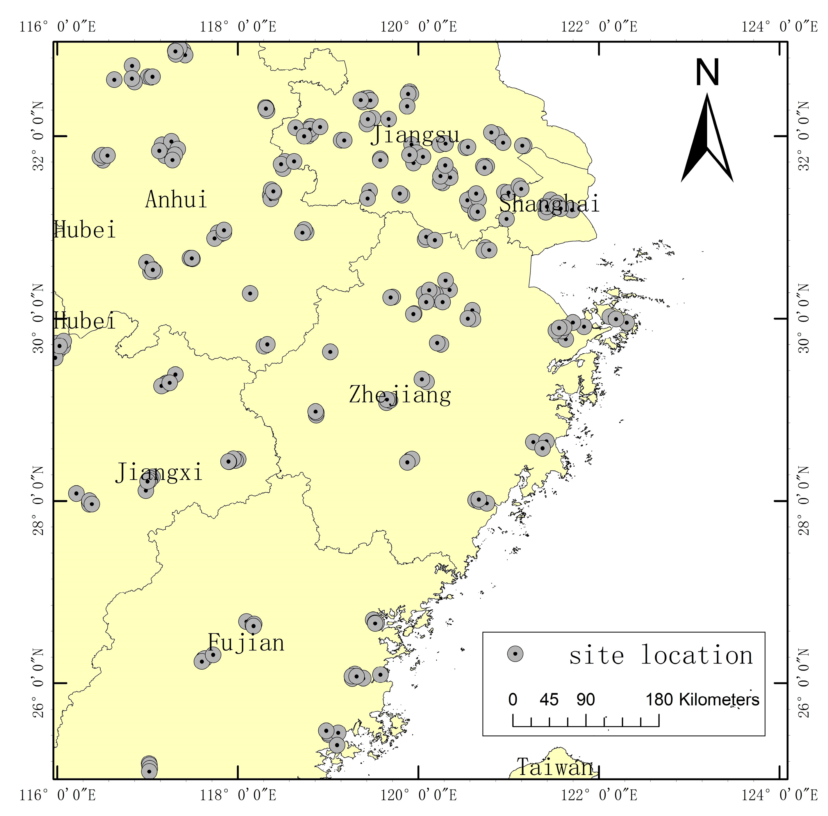
This study obtained the hourly NO2 observation data from May 2018 to December 2020 from the China Environmental Monitoring Center (CEMC). All sites are based on the GB3095-2012 standard, and the near-ground NO2 concentration is measured by the chemiluminescence method [30]. The study area is the coastal area (116–124°E, 25–33°N) with the main cities of the Yangtze River Delta as the core. There are 258 monitoring stations within the range, most of which are located in urban areas, and a few are located in suburban areas (Figure 1). In order to build a high-precision NO2 exposure assessment model, we averaged the hourly NO2 observation records to the day, eliminated daily observation data of less than 18 h, and finally obtained 225,197 valid observation records.
2.1.2. TROPOMI NO2 Data
The TROPOspheric Monitoring Instrument (TROPOMI) can monitor the data of air pollutants such as NO2, O3, SO2, and HCHO. The time when the satellite passes through the study area (Beijing time) is about 13:00–14:00, and the spatial resolution is 7 km × 3.5 km (30 April 2018 to 6 August 2019) and 5.5 km × 3.5 km (7 August 2019 to now), making it the best atmospheric observation spectrometer at present. Under the processing framework of the retrieval–assimilation–modeling system, the TROPOMI NO2 Level 2 product combines the DOAS algorithm and the TM5 chemical transport model, and converts the measured Level-1B radiance and irradiance spectra into NO2 vertical column concentrations, in units of molec/cm2 [24]. For this article, the TROPOMI NO2 Level 2 product from NASA (https://disc.gsfc.nasa.gov/, accessed on 7 July 2021) was obtained and the tropospheric NO2 column concentration was taken from it as a modeling factor. To weaken cloud cover, snow landscapes, and other dubious retrievals, we kept the pixels in the file that had a quality assurance value (QA) greater than 0.75. Data missing more than 30% were also removed, as too many missings would increase uncertainty.
2.1.3. Meteorological Data
To include the influence of near-surface meteorological conditions on the potential chemical and physical processes of NO2 in the atmosphere, we obtained the daily average air pressure, air temperature, relative humidity, land surface temperature, 24 h cumulative rainfall, and wind speed from China’s National Meteorological Data Center (http://data.cma.cn/, accessed on 23 July 2021).
2.1.4. The Reanalysis Data
We also obtained ERA5 reanalysis data for 2018–2020 from the European Centre Medium-Range Weather Forecasts (ECMWF), which combined past observations with models to simulate hour-by-hour atmospheric, ocean wave, and land surface quantities systematically. In order to assist in the establishment of an exposure assessment model between satellite-observed NO2 and ground-level NO2, we selected 22 indicators from the ERA5 data, including radiation, heat, atmospheric conditions, and wind fields, which may affect changes in NO2 concentration (Table S1). According to the physical meaning of the different indicators, the daily data of each indicator are generated by summing or averaging, with a resolution of 0.25° × 0.25°.
2.1.5. Geographical Variable Data
Human activities and the distribution of emission sources are also important factors affecting regional NO2 changes. Transportation activities and industrial production activities are the main reasons for the uneven distribution of NO2 in space, and geographical features are closely related to these activities and also affect the spatial distribution of near-ground NO2 concentrations to a certain extent [26,31,32]. Therefore, we selected five parameters of the geographic environment, including elevation data (DEM), vegetation index data (NDVI/EVI), road network data (L), gridded population data (POP), and land cover data (LAND), to characterize these effects.
Among these, the 300 m land cover data come from the Climate Change Initiative (CCI) project of the European Space Agency (ESA, http://maps.elie.ucl.ac.be/CCI/viewer/index.php, accessed on 4 March 2021). This study reclassified the 22 types of land in the original data from 2018 to 2020 into six types: forest land, grassland, agricultural land, urban land, water bodies, and other land, and calculated the area within a grid range of 0.03° and the proportion of each. The road network data were downloaded from OpenStreetMap (OSM, http://download.geofabrik.de/asia/china.html#, accessed on 19 March 2021), and we calculated the road network length and road network density within a 0.03° grid range year by year.
In addition, we also processed the MODIS vegetation index data (MOD13A2), the 90 m DEM data of SRTM, and the grid population data of Worldpop. Detailed data descriptions and sources can be seen in the modeling variable pre-selection table (Table S1). All variables may affect the NO2 concentration but may not be necessary for high-precision NO2 exposure assessment modeling.
2.1.6. Data Integration
In order to unify the explanatory variables with different scales from multiple sources, we constructed a 0.03° × 0.03° (about 3 km) grid mesh, and integrated all data on the basis of this standard. For data with a spatial resolution lower than 0.03°, the inverse distance weighting method (IDW) was used to interpolate them into the mesh; for the data with a spatial resolution higher than 0.03°, we used resampling technology to upscale it into the standard mesh. By matching the geographic locations of the NO2 ground observation sites, all the data finally formed a dataset for modeling and validation.
2.1.7. Feature Selection
In both traditional statistical models and machine learning models, too many explanatory variables are an important factor causing model instability [33,34]. Although machine learning is better at learning the nonlinear relationship between variables and weakens the effect of collinearity between similar variables to a certain extent, it is still necessary to reduce similar and unnecessary predictors. By considering the Pearson correlation coefficient between the variables (Figure S1a,b), we initially screened the explanatory variables with low correlations with near-ground NO2 concentrations and deleted explanatory variables with similar physical meanings and a high correlation between each other (|r| > 0.95) on the premise of ensuring the completeness of the predictor system.
Finally, the NO2 column concentration (NO2_5p), air pressure (AP), land surface temperature (LST), relative humidity (HD), rainfall (RF), boundary layer height (BLH), surface latent heat flux (SLHF), lower surface solar radiation (SSRD), top net solar radiation (TSR), 10 m wind speed (U10/V10), total column ozone (TCO3), road network density (ROAD_E), elevation (DEM), population (POP), vegetation index (EVI), the proportion of grassland (GLA_P), the proportion of forest land (tree_p), the proportion of agricultural land (AGR_P), and the proportion of urban land (CITY_P) were used as the basic predictors. By combining these with the meteorological hysteretic effects term and the spatiotemporal term proposed in Section 2.2, we improved the underlying predictors and formed the final set of predictors for the model.
2.2. Methodology
2.2.1. Hysteretic Effects Term
Meteorological conditions often have a continuous impact on atmospheric pollutants. Over time, a change in the mechanism of influence or the accumulated effects of the influence may increase the magnitude of the influence, usually called the hysteretic effects. Examples include the chemical accumulation process of temperature-induced changes in atmospheric pollutant concentrations [35] and the interaction mechanism between the short-term wet deposition of trace gases by rainfall and the hydrolysis of pollutants such as formaldehyde polymers in a humid atmospheric environment [36]. These physicochemical processes create a certain hysteresis effect.
Therefore, in this study, we bundled the meteorological predictors observed at the site with the records of the previous 2 days and used them as the meteorological hysteretic effects to construct a NO2 exposure assessment model, which is conducive to solving the problem that the single-day variables cannot fully characterize the characteristics of the change in NO2 concentration due to the hysteretic impact. The details are shown in Equation (1):
where is the meteorological hysteretic effects term of day , and and are the meteorological factors of day and the previous two days, respectively.
2.2.2. Spatiotemporal Term
The spatiotemporal distribution of NO2 concentrations is highly spatially heterogeneous, as is the case for other air pollutants, such as formaldehyde and PM2.5. Spatially, the NO2 concentration varies with location and exhibits different statistical relationships with covariates. Incorporating spatial information into the model can effectively capture the spatial variation in the target gas pollutants. Methods such as geographic weighted regression [37] and spatiotemporal geographic weighted regression [38,39] use spatial coordinates to capture spatial heterogeneity. However, spatial coordinates are absolute coordinates of the world as a whole. In applying machine learning methods directly to a small- and medium-scale regions, it may not be able to explain spatial nonstationarity and spatial autocorrelation well. Therefore, for this study, we calculated the Vincenty relative ellipsoid distance from the sample location to the lower left corner (116°E, 25°N) and the upper right corner (124°E, 33°N) of the study area in the WGS84 coordinate system [40] as the spatiotemporal terms, which are reflected in Equation (2). Studies have shown that machine learning models built with field distance as a spatial factor have a good ability to capture spatially heterogeneous features [41,42]. In terms of time, the NO2 concentration showed a strong cyclical trend, basically showing the characteristics of being high in spring and winter, and low in summer and autumn (Figure S2). Therefore, we constructed a time factor of months and introduced this rule into the model to improve the performance of the NO2 exposure assessment model. See Equation (3) for details.
where is the spatial term at the grid’s center point, is the geographic coordinates of the center of a grid point, is the geographic coordinates of the lower left corner of the study area, is the geographic coordinates of the upper right corner of the study area, represents an iterative function of the ellipsoid distance, represents the temporal heterogeneity factor for month , and represents month i.
2.2.3. Ensemble Model
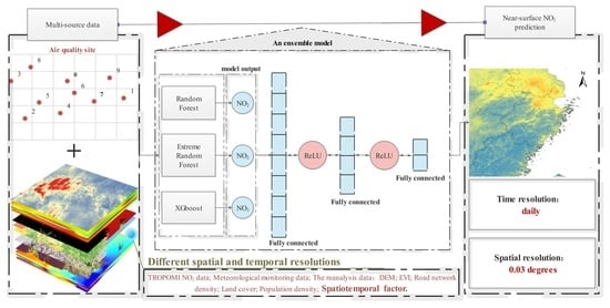
Our study adopted a “Classic Machine Learning + Deep Neural Network“ ensemble model to evaluate the near-ground NO2 concentrations. First, we constructed a statistical relationship between the explanatory variables and the NO2 concentrations based on three machine learning models: Random Forest (RF), Extreme Random Forest (EXT), and XGboost (XGB). These three models are all based on regression trees, which can learn the nonlinear relationships among variables very well. However, due to the differences in their principles, the deviation and variance in the predicted results will also be quite different. Both RF and EXT are ensemble learning models based on the bagging strategy: they randomly select prediction samples to increase the generalization of the model [43]. On the other hand, XGB is a boosting ensemble learning method and its base learners are related to each other, which can maximize the model’s accuracy, although this will reduce the generalizability to a certain extent [44]. Considering the prediction performance and generalization ability of the model, the key hyperparameters of the three algorithms were optimized with grid search. For RF and EXT, the number of trees (n_estimators) and the tree depth (max_depth) were set to 150 and 25, respectively; for XGB, the number of trees (n_estimators) and the tree depth (max_depth) were set to 500 and 13, respectively. In order to prevent the model overfitting, we also set the gamma coefficient to 1.
Finally, in order to integrate and optimize the prediction results of these machine learning methods, we inputted their prediction results into a deep learning network composed of 3 fully connected layers and 2 ReLU layers, and realized the near-ground NO2 concentration exposure assessment. All models were implemented by the pytorch and scikit-learn packages, and the detailed structure is shown in Figure 2.
2.2.4. Model Validation
In the 10-fold cross-validation technique (10-fold CV), the dataset is randomly divided into 10 data subsets and 1 data subset is selected in turn for model validation, with the remaining 9 used for model establishment. The final evaluation of the 10-fold CV results is the average of the 10 time validations, which can more realistically evaluate the model’s performance. To evaluate the fitting performance and generalization performance of the ensemble model, we used the 10-fold cross-validation technique to calculate the R2 (goodness of fit), MAE (mean absolute error), and RMSE (root-mean-square error). The details are shown in Equations (4)–(7).
where are the true value and the model’s predicted value for the ith sample, respectively, is the average value of whole sample, and is the jth cross-validation result of the statistic.
3. Results
3.1. Model Development and Validation
3.1.1. Analysis of the Impact of Enhanced Variables on the Model
In order to explore the influence of the spatiotemporal term and the hysteretic effects term on the model, we designed four variable combination schemes and used the CV verification method to analyze the performance of different independent variable schemes in the RF, EXT, and XGB models, which are shown in Table 1. The results show that the CV R2 of the three machine learning models were significantly improved when the two model enhancement factors were added separately (Plan2 and Plan3). In particular, when the spatiotemporal term was added, the R2 of the RF, EXT, and XGB models reached 0.81, 0.82, and 0.88, meaning that the performance of the three models was improved by 4%, 4%, and 6%, respectively. When the meteorological hysteretic effects term and the spatiotemporal term were added at the same time, the performance of each machine learning model still increased slightly with an increase in the explanatory variables, and the R2 range was 0.82–0.88. Under the same scheme, the performances of the three models were ranked in descending order as XGB, EXT, and RF.
Figure S3a–d show the relative importance of the independent variables for the four schemes. When no model enhancement variables were introduced (Figure S3a), TROPOMI NO2 was the most important factor (RF: 35%, EXT: 25%, XGB: 25%), followed by air pressure (AP) and boundary layer height (BLH), which were two or three times less important than TROPOMI NO2 concentrations. When the meteorological hysteretic effect term was introduced into the model (Figure S3b,d), its relative importance in all models was 2–14%. The relative importance of air pressure and land surface temperature two days ago was higher than that of the current day, which indicates that the meteorological hysteretic effects term is better than the simple meteorological factor. When the spatiotemporal term was introduced into the model (Figure S3c,d), the temporal heterogeneity factor became one of the most important factors (7–20%), second only to TROPOMI NO2. Overall, although there were some differences in the relative importance of the variables in different models, TROPOMI NO2, boundary layer height, the meteorological hysteretic effects term, and the spatiotemporal term had important effects in all models.
3.1.2. Model Evaluation
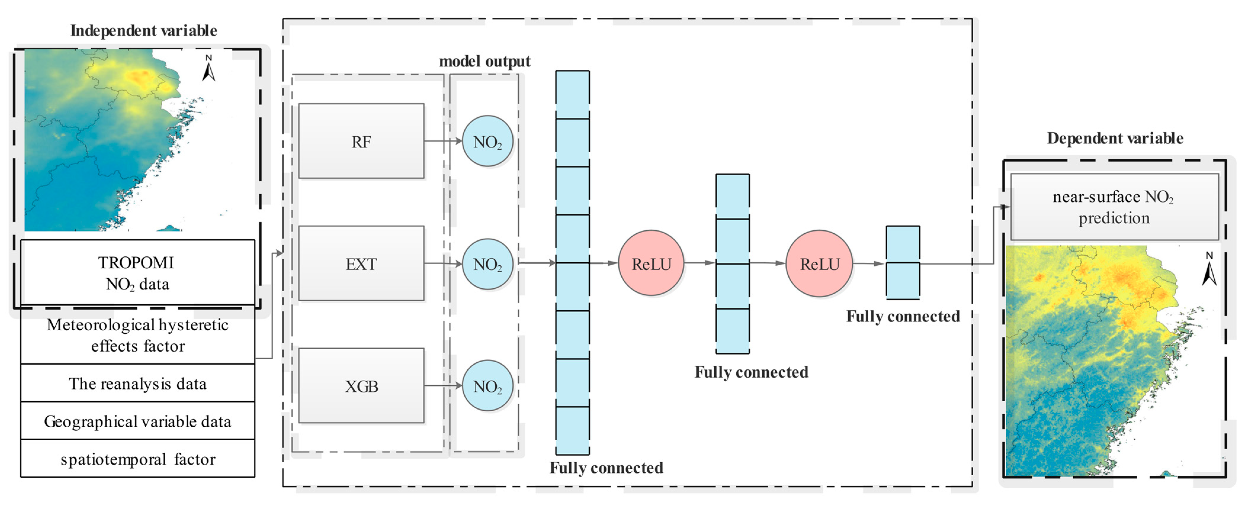
We finally constructed a near-ground NO2 concentration exposure assessment model based on the variable system of Plan 4. Figure 3 shows the CV results of the six models. The RMSE values of the multiple linear, SVM, RF, EXT, XGB, and ensemble models were 11.88, 7.56, 7.22, 6.76, 5.71, and 5.62 µg/m3, and the corresponding MAE values were 9.20, 5.43, 5.26, 4.91, 4.11, and 4.04 µg/m3, respectively. The 10-fold cross-validation R2 of the ensemble model was 0.89, which was significantly better than the multiple linear model (CV R2: 0.51) and the SVM model (CV R2: 0.80). The RF, EXT, and ensemble models overestimated the near-ground NO2 concentration, and the SVM, multiple linear, and XGB models underestimated the near-surface NO2 concentration. Overall, the ensemble model corrected the predictions of the different machine learning models through the deep learning network and outperformed the individual machine learning models.
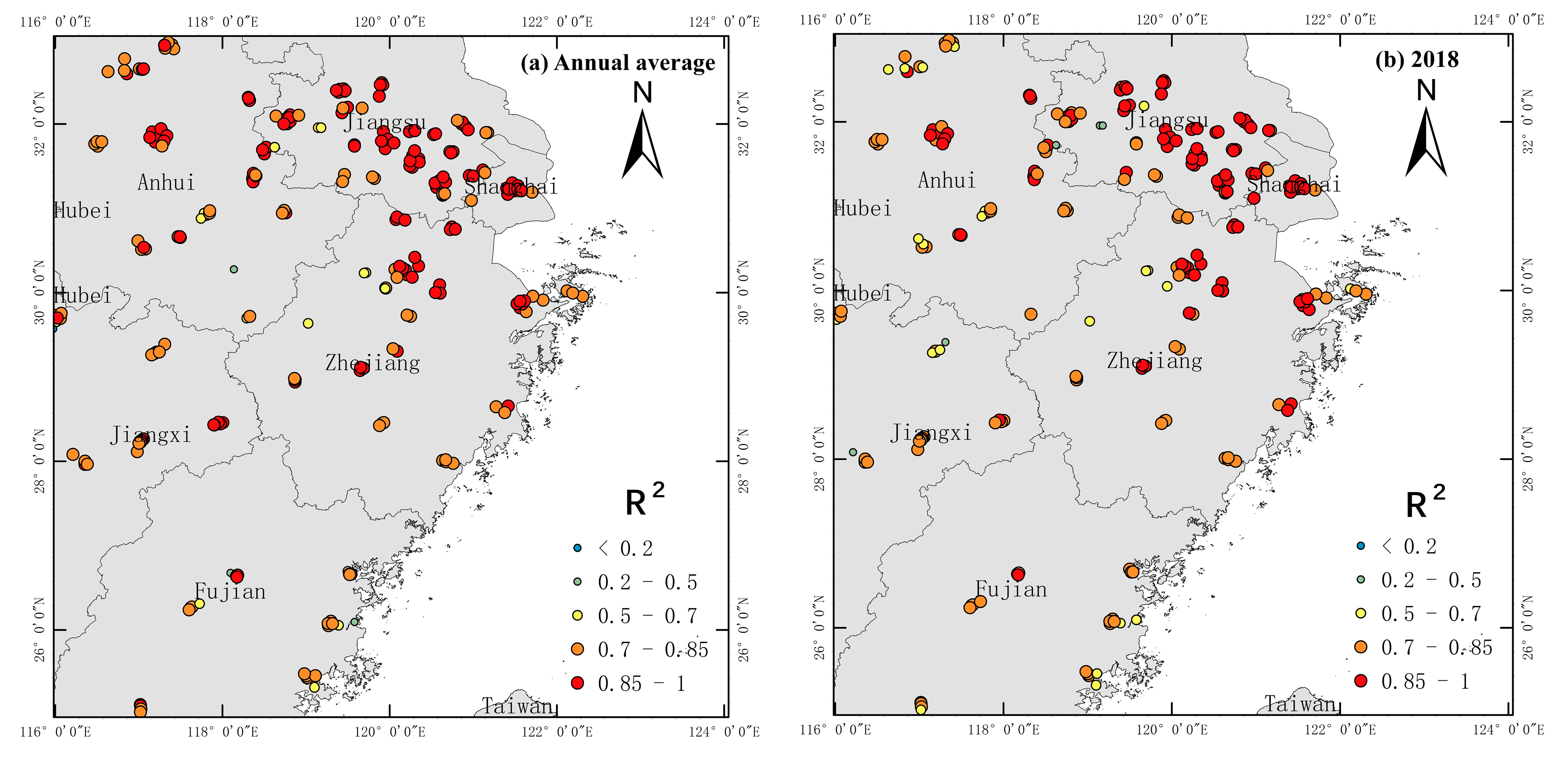
Figure 4 shows the local R2 distribution information. Spatially, the local R2 of the annual statistical scale and the full-time statistical scale have similar regional distribution characteristics. The local R2 is high in the areas with a large population and densely distributed monitoring stations, while the local R2 in the areas with a small population and sparsely distributed stations is low. In the case of sparse sites, it is difficult for the model to fully explore the statistical relationship between the NO2 concentration and the explanatory variables. Across the entire study period, the range of local R2 is 0.13–0.94, and 92% of the sites have a local R2 of >0.7. This result is consistent with the performance results of local RMSE (Figure S4) and MAE (Figure S5), which means that the model has a relatively stable fitting performance.
We also captured the model prediction results for different site locations and plotted the trend of changes in the daily average NO2 concentration from May 2018 to December 2020 (Figure S6). In the time series, the predicted results are basically consistent with the actual observed results (Figure S2), and there is no obvious deviation, indicating that the model shows high stability for the time series.
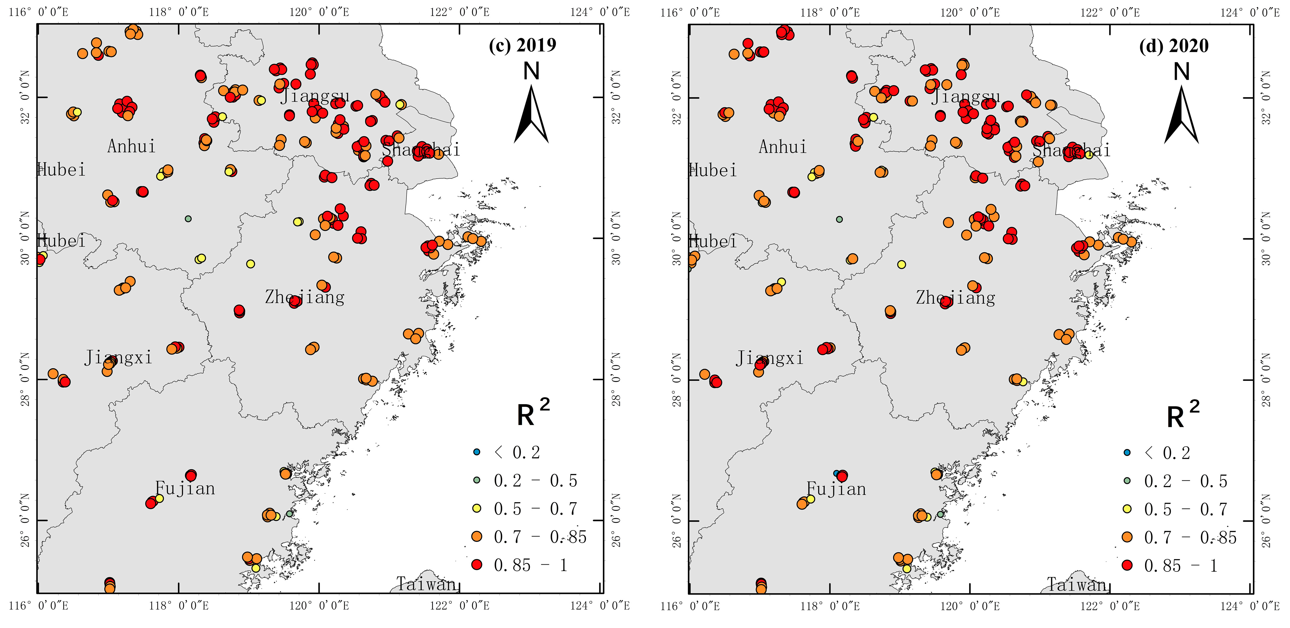
Based on the ensemble model framework, three validation sets were designed in this study, namely all samples in the last 3 months of 2020, 30% randomly selected samples from all sites, and 30% randomly selected samples. These validation sets did not participate in model training, and their validation results represent the temporal, spatial, and comprehensive predictive capabilities of the model, respectively, as detailed in Figure 5. The ensemble model had the strongest comprehensive prediction ability (Figure 5a), with an R2 of 0.86 between the predicted value and the true value, which means that the model was able to predict 86% of the near-ground NO2 concentrations. The performance of the model for temporal (Figure 5b) and spatial (Figure 5c) variations was slightly weaker than the comprehensive prediction ability, but it still showed a relatively good spatiotemporal prediction ability and applicability. The temporal and spatial R2 values of the model reached 0.71 and 0.81, respectively, and the corresponding RMSE and MAE were 10.24 µg/m3, 7.79 µg/m3, 7.39 µg/m3, and 5.50 µg/m3. Compared with the XGBoost model (Figure 5d–f), the comprehensive prediction R2, temporal R2, and spatial R2 of the ensemble model were improved by 1%, 2%, and 1%, respectively, and the corresponding RMSE was reduced by 0.23 µg/m3, 0.19 µg/m3, and 0.23 µg/m3.
3.2. Analysis of the Fine-Scale Spatiotemporal Variation in NO2
To analyze the ability of the ensemble model of capturing the spatially heterogeneous features, we interpolated the satellite-observed tropospheric NO2 vertical column concentrations to a spatial resolution of 0.03° and compared it with the ensemble model’s output of the spatial distribution of the near-surface NO2 concentration (Figures S7 and S8). The spatial distribution law of the model output and the interpolation results of satellite observations were basically consistent, which proves the correctness of the model output results from a new perspective. In detail, the interpolation results of the satellite observations were relatively smooth. Although the spatial resolution after interpolation was consistent with the model output, the degree of step difference between adjacent pixels was not obvious. Especially in Ningbo, Fuzhou, Wenzhou Province, and other areas with a small area of high NO2 concentrations, as well as the median NO2 concentration between mountainous areas, satellite observations cannot easily capture the spatial heterogeneity. The smoothing effect is outstanding. In contrast, the NO2 concentration results of the model showed obvious step differences, whether in urban areas with higher NO2 concentrations, such as Shanghai, or in mountainous areas with lower NO2 concentrations, such as southern Zhejiang Province; these features were directly smoothed in the satellite observations. Therefore, the results of the ensemble model reflect the spatial heterogeneity of the near-ground NO2 concentration.
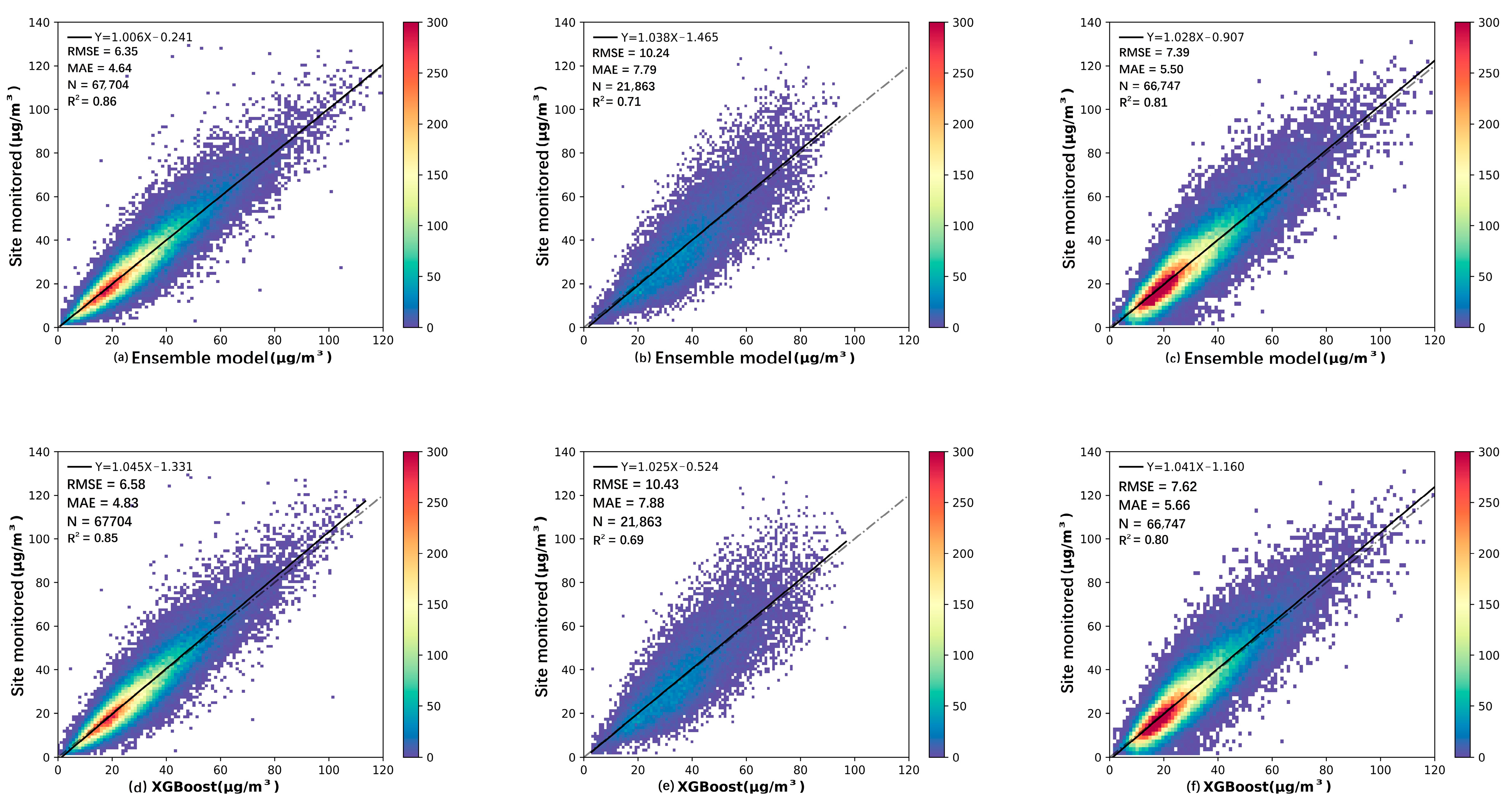
Figure 6 shows the seasonal distribution of NO2 concentrations over the studied area. In Figure S9, the temporal variation in the characteristics of the NO2 concentration across different seasons is obvious, while the spatial distribution characteristics are similar. The average concentration of NO2 near the ground, from largest to smallest, is: winter (22.51 µg/m3), autumn (18.89 µg/m3), spring (17.76 µg/m3), and summer (11.91 µg/m3), which is consistent with Pan et al.’s study on the Chinese region [45]. Spatially, the near-surface NO2 concentrations are high in the north and low in the south, and have a decreasing trend from the coast to the inland areas. The high-value areas are mainly distributed in the north of Zhejiang Province, Anhui Province, Jiangsu Province, and Shanghai. It is worth noting that the average NO2 concentration level across the four seasons is not high, which is because there are a large number of suburban and rural areas in our research region, and the NO2 concentration in these areas is at a low level. In fact, NO2 concentrations in urban areas are still at relatively high levels. Coal-fired heating and natural seasonal conditions of unfavorable diffusion are important factors leading to this phenomenon [45].
3.3. Analysis of Near-Surface NO2 Concentrations in Major Cities
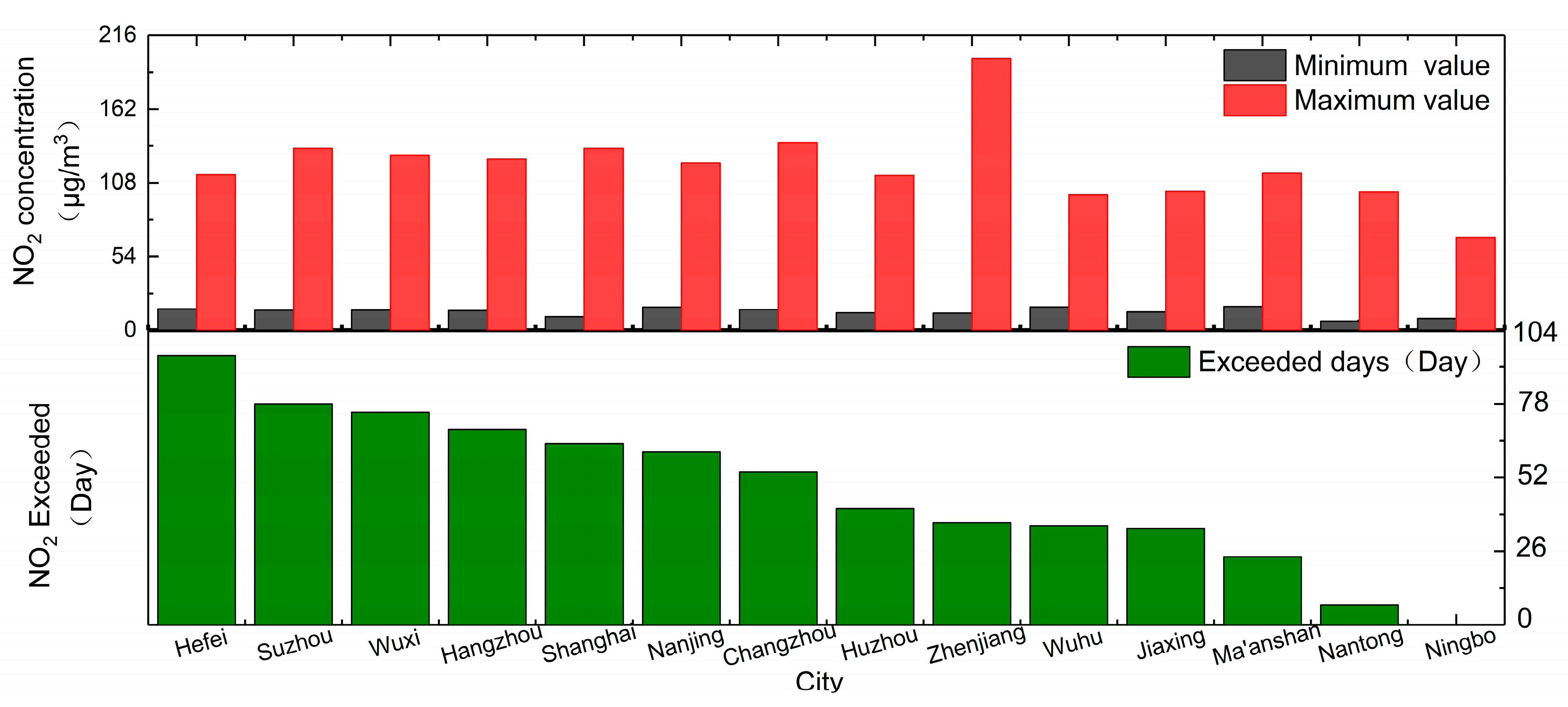
As a typical area with a high near-surface NO2 concentration in the study area, the Yangtze River Delta Plain has a large population base and complex human activities, and is also one of the most important economic areas in China. In accordance with the national ambient air quality standard GB 3095-2012, we calculated the NO2 air quality of major cities in the Yangtze River Delta Plain with a daily average NO2 concentration of >80 µg/m3. If any grid in the city did not meet the national regulations, it was considered to have exceeded the standard. The details are shown in Figure 7.
Between 28 April 2018 and 31 December 2020, Hefei was the city most seriously polluted by NO2, with 95 days of air NO2 exceeding the standard. In addition, Suzhou, Wuxi, Hangzhou, Shanghai, and Nanjing had more than 60 days exceeding the standard, and the corresponding maximum NO2 concentration was also relatively high, indicating that the air quality of these cities was relatively poor. It is worth noting that when NO2 air pollution occurs, the near-surface NO2 concentration in Zhenjiang and Changzhou can reach very high levels (greater than 135 µg/m3), although the number of days when this occurs is not particularly great, indicating that the two cities need to be alert to the occurrence of sudden NO2 air pollution incidents. Among the many cities in the Yangtze River Delta Plain, only Ningbo City did not have the phenomenon of excessive NO2 concentrations in the air.
All in all, there is still much room for improvement in the air quality of major cities in the Yangtze River Delta Plain. Most of these places have relatively developed economies, a large population, and low terrain. Anthropogenic emissions may be the main reason for the formation of these high-value areas. In recent years, a series of effective measures for environmental governance have reduced the average concentration of NO2 in the entire region, but the effect has not been significant. It is still necessary to implement targeted prevention and control measures for cities with more serious pollution.
4. Discussion
Focusing on the scientific issue of assessing near-surface NO2 concentrations, we designed a model enhancement factor considering the influencing mechanism of multi-source explanatory variables on the near-surface NO2 concentration and the spatial heterogeneity in NO2 concentration itself. With an ensemble model composed of a deep neural network and machine learning methods, a high-precision ground NO2 concentration exposure assessment model was developed.
Compared with previous studies, our model exhibits certain advantages. The ensemble model in this study has a better ability to evaluate the NO2 concentrations, and its R2 in the 10-fold cross-validation results is 0.89, which is better than the performance of most models, such as the annual-scale stepwise regression model (CV R2: 0.78) constructed by Xu et al. [46], the seasonal-scale land use regression model (CV R2: 0.70) constructed by Zhang et al. [23], the annual-scale land use regression model (CV R2: 0.67) constructed by Andrew Larkin et al. [47], the monthly scale random forest model in China constructed by You et al. [27] (CV R2: 0.85), the daily-scale random forest and extreme random forest models constructed by Qin et al. [43] (CV R2: 0.70 and 0.72), the XGBoost daily-scale model (CV R2: 0.83) constructed by Liu [29], and the random forest spatiotemporal kriging (RF-STK) model (CV R2: 0.62) constructed by Zhan et al. [48]. At the same time, the model in this article outputs daily-scale results with a spatial resolution of 0.03° (about 3 km), which can better meet the needs of research such as popular medicine and environmental protection. As far as we know, there are not many daily-scale NO2 exposure assessment models with a spatial resolution better than 0.03° in China. Only the random forest model constructed by Pan et al. [45] and the ensemble model (Machine Learning + GAM) constructed by Huang et al. [26] and Di et al. [49] reached a spatial resolution of 1 km, but the performance of these models (CV R2: 0.67–0.82) was slightly lower than that of the model in this study. The prediction performance of our model was also good: The spatial prediction R2 and the temporal prediction R2 were 0.81 and 0.71 respectively, which is slightly weaker than the model with the best temporal prediction ability of the abovementioned studies (Di et al. [49], spatial prediction R2: 0.84, temporal prediction R2: 0.73).
Multi-source predictors and their effective utilization are the keys to improving model performance. As in most studies [29,43], the TROPOMI tropospheric NO2 column concentration was the most important predictor in this model because it has a consistent trend with near-surface NO2 concentrations (Figure S2). Compared with OMI-NO2 (the NO2 observed by the Ozone Monitoring Instrument), the NO2 exposure assessment models constructed with TROPOMI-NO2 had better accuracy, which was demonstrated in the study of Liu et al. [29]. We also designed a meteorological hysteretic effects term and a spatiotemporal term. When used alone, they significantly improved the model’s performance (accuracy improvement: 4–6%) and played an important role in the explanatory variable system (Figure S1), which is consistent with previous studies in China [42,45]. However, when the meteorological hysteretic effects term and the spatiotemporal term were used at the same time, the performance of the model was not improved significantly, which may be because the accuracy of the model itself had reached a high level, and there were systematic errors in the explanatory variables themselves. In addition, the atmospheric condition variables and other geographic factors in the hourly climate analysis data also play a role to varying degrees. Although the relative importance of these variables is not high enough to significantly improve the model’s performance, they increase the spatial heterogeneity of the model. For example, DEM, city proportion, road network density, and population are highly consistent with the predicted spatial distribution of NO2 concentrations.
The systematic and comprehensive multi-source explanatory variable system also increases the interpretability and applicability of the model. It contains large-scale data sources at fine spatial scales, giving the model the potential to produce higher-spatial-resolution NO2 products (better than 1 km) and apply them to larger areas. In future studies, the model is also expected to be applicable to other high-level exposure assessment models for atmospheric pollutants that have both site and satellite observations.
However, there are still some limitations of our study. First, although the model proposed in this article has a good temporal prediction ability (R2: 0.71), this is only a short-term prediction, and the stationarity of the long-term prediction of the model needs to be further explored and proved. Second, the performance of the model and the potential for application of the model at higher time scales are limited due to the coarse resolution of the geographic data and atmospheric condition data. On the one hand, the spatial resolution of the analytical data (ERA5) used by the model is 0.25°, and a single pixel record is not enough to perfectly describe the atmospheric conditions at the site location, which increases the uncertainty of the model. On the other hand, at a fine spatiotemporal scale (hourly scales, 100 m level resolution), the information provided by TROPOMI NO2 and the meteorological data will not be sufficient to reflect the short-term changes in NO2 concentration caused by transportation, daily life, and industrial emissions. Variations in human activity at a fine enough spatial and temporal resolution are needed to provide relevant information. Currently, such data are difficult to obtain and are not publicly available, which means that it is difficult for the model to improve in terms of temporal resolution. Third, the meteorological hysteretic effects term proposed in this article only considers the meteorological factors over 3 days. This assumption is too simple and may limit the further improvement of the model’s performance. The time span involved in the hysteretic effects may be more than 3 days and is not fixed. In future research, developing a dynamic hysteretic effects term will help to improve the model.
5. Conclusions
In this article, we combined the XGB, RF, EXT, and deep neural network models, and used multi-source data to develop a high-precision ensemble model, which was successfully applied to the central and southern coastal areas of China, generating a near-ground daily average NO2 concentration distribution of 0.03°. Compared with other studies, the ensemble model had better estimation accuracy, with 10-fold CV R2, RMSE, and MAE values of 0.89, 5.62 µg/m3, and 4.04 µg/m3, respectively.
The model has good generalization in space and time, and the short-term daily average NO2 prediction effects were stable and reliable, which shows that the model can be applied to larger areas and longer time series. Compared with satellite observations and site observations, the ensemble model output provides rich and accurate details of the spatiotemporal heterogeneity in NO2, which will be helpful for air pollutant traceability and urban health research in the future.
Supplementary Materials
The following supporting information can be downloaded at: https://www.mdpi.com/article/10.3390/rs14122807/s1, Table S1: Modeling variable preselection table; Figure S1: Pearson correlation between the near-ground NO2 concentrations and the explanatory variables; Figure S2: Time variation trend of NO2 concentrations observed by TROPOMI and ground stations; Figure S3: The relative importance of explanatory variables in the three machine learning methods of XGB, EXT, and RF: (a) the relative importance of variables in Plan 1; (b) the relative importance of variables in Plan 2; (c) the relative importance of variables in Plan 3; (d) the relative importance of variables in Plan 4; Figure S4: Spatial distribution of the local RMSE values of the ensemble model; Figure S5: Spatial distribution of the local MAE values of the ensemble model; Figure S6: The daily average variation in NO2 concentrations outputted by the ensemble model; Figure S7: The distribution of the daily average NO2 concentrations outputted by the ensemble model; Figure S8: The distribution of daily average tropospheric NO2 column concentrations interpolated from TROPOMI observations; Figure S9: The monthly and annual average variation in NO2 concentrations outputted by the ensemble model.
Author Contributions
Conceptualization, S.H., H.D. and Y.Y.; methodology, S.H.; software, S.H.; validation, S.H., H.D. and Y.Y.; formal analysis, S.H. and H.D.; resources, H.D. and Y.Y.; data curation, Z.Z.; writing—original draft preparation, S.H.; writing—review and editing, H.D. and Y.Y.; visualization, Z.Z.; supervision, H.D. and Y.Y.; project administration, H.D.; funding acquisition, H.D. All authors have read and agreed to the published version of the manuscript.
Funding
This research was funded by the National Natural Science Foundation of China (52079101), the Zhejiang Ecological Environment Research and Achievement Promotion Project (2020HT0011), and the Ningbo Science and Technology Plan Project (2021ZH1CXYD060013).
Acknowledgments
The authors thank NASA for providing free TROPOMI NO2 data and vegetation index data, the European Space Agency for providing ERA5 reanalysis data, the National Meteorological Science Data Center for providing meteorological data, the China Environmental Monitoring Center for providing ground-level NO2 observation data, the Climate Change Initiative for providing land cover data, SRTM for providing DEM data, OSM for providing road network data, and Worldpop for providing population data.
Conflicts of Interest
The authors declare no conflict of interest.
References
- Kim, H.C.; Lee, P.; Judd, L.; Pan, L.; Lefer, B. OMI NO2 column densities over North American urban cities: The effect of satellite footprint resolution. Geosci. Model Dev. 2016, 9, 1111–1123. [Google Scholar] [CrossRef]
- Palmer, P.I.; Jacob, D.J.; Fiore, A.M.; Martin, R.V.; Chance, K.; Kurosu, T.P. Mapping isoprene emissions over North America using formaldehyde column observations from space. J. Geophys. Res. Atmos. 2003, 108, 4180. [Google Scholar] [CrossRef]
- Jacob, D.J.; Heikes, E.G.; Fan, S.M.; Logan, J.A.; Mauzerall, D.L.; Bradshaw, J.D.; Singh, H.B.; Gregory, G.L.; Talbot, R.W.; Blake, D.R.; et al. Origin of ozone and NOx in the tropical troposphere: A photochemical analysis of aircraft observations over the South Atlantic basin. J. Geophys. Res. Atmos. 1996, 101, 24235–24250. [Google Scholar] [CrossRef]
- Gifford, F. Atmospheric Chemistry and Physics of Air Pollution. Eos Trans. Am. Geophys. Union 1987, 68, 1595. [Google Scholar] [CrossRef]
- Fishman, J.; Crutzen, P.J. The origin of ozone in the troposphere. Nature 1978, 274, 855–858. [Google Scholar] [CrossRef]
- Chen, R.; Samoli, E.; Wong, C.M.; Huang, W.; Wang, Z.; Chen, B.; Kan, H.; Group, C.C. Associations between short-term exposure to nitrogen dioxide and mortality in 17 Chinese cities: The China Air Pollution and Health Effects Study (CAPES). Environ. Int. 2012, 45, 32–38. [Google Scholar] [CrossRef]
- Gauderman, W.J.; McConnell, R.; Gilliland, F.; London, S.; Thomas, D.; Avol, E.; Vora, H.; Berhane, K.; Rappaport, E.B.; Lurmann, F.; et al. Association between air pollution and lung function growth in southern California children. Am. J. Respir. Crit. Care Med. 2000, 162, 1383–1390. [Google Scholar] [CrossRef]
- Faustini, A.; Rapp, R.; Forastiere, F. Nitrogen dioxide and mortality: Review and meta-analysis of long-term studies. Eur. Respir. J. 2014, 44, 744–753. [Google Scholar] [CrossRef]
- Jerrett, M.; Burnett, R.T.; Beckerman, B.S.; Turner, M.C.; Krewski, D.; Thurston, G.; Martin, R.V.; van Donkelaar, A.; Hughes, E.; Shi, Y.; et al. Spatial analysis of air pollution and mortality in California. Am. J. Respir. Crit. Care Med. 2013, 188, 593–599. [Google Scholar] [CrossRef]
- Wang, W.N.; Cheng, T.H.; Gu, X.F.; Chen, H.; Guo, H.; Wang, Y.; Bao, F.W.; Shi, S.Y.; Xu, B.R.; Zuo, X.; et al. Assessing Spatial and Temporal Patterns of Observed Ground-level Ozone in China. Sci. Rep. 2017, 7, 3651. [Google Scholar] [CrossRef]
- Sun, J.; Zhou, C.Y.; Zhang, Y.H.; Yang, X.Y.; Ge, L.; Liu, J.J. Spatio-temporal variation of tropospheric NO2 column density in Shan dong Province nearly five years. Environ. Sci. Technol. 2021, 44, 177–182. [Google Scholar] [CrossRef]
- Martin, R.V. Evaluation of GOME satellite measurements of tropospheric NO2 and HCHO using regional data from aircraft campaigns in the southeastern United States. J. Geophys. Res. 2004, 109, D24307. [Google Scholar] [CrossRef]
- Wang, H.; Wei, W.; Che, H.; Tang, X.; Bian, J.; Yu, K.; Wang, W. Ground-Based MAX-DOAS Measurements of Tropospheric Aerosols, NO2, and HCHO Distributions in the Urban Environment of Shanghai, China. Remote Sens. 2022, 14, 1726. [Google Scholar] [CrossRef]
- Levelt, P.F.; Van Den Oord, G.H.J.; Dobber, M.R.; Malkki, A.; Visser, H.; De Vries, J.; Stammes, P.; Lundell, J.O.V.; Saari, H. The ozone monitoring instrument. IEEE Trans. Geosci. Remote Sens. 2006, 44, 1093–1101. [Google Scholar] [CrossRef]
- Rabiei-Dastjerdi, H.; Mohammadi, S.; Saber, M.; Amini, S.; McArdle, G. Spatiotemporal Analysis of NO2 Production Using TROPOMI Time-Series Images and Google Earth Engine in a Middle Eastern Country. Remote Sens. 2022, 14, 1725. [Google Scholar] [CrossRef]
- van der A, R.J.; Mijling, B.; Ding, J.; Koukouli, M.E.; Liu, F.; Li, Q.; Mao, H.; Theys, N. Cleaning up the air: Effectiveness of air quality policy for SO2 and NOx emissions in China. Atmos. Chem. Phys. 2017, 17, 1775–1789. [Google Scholar] [CrossRef]
- Cyrys, J.; Eeftens, M.; Heinrich, J.; Ampe, C.; Armengaud, A.; Beelen, R.; Bellander, T.; Beregszaszi, T.; Birk, M.; Cesaroni, G.; et al. Variation of NO2 and NOx concentrations between and within 36 European study areas: Results from the ESCAPE study. Atmos. Environ. 2012, 62, 374–390. [Google Scholar] [CrossRef]
- Kim, H.; Lee, S.-M.; Chai, T.; Ngan, F.; Pan, L.; Lee, P. A Conservative Downscaling of Satellite-Detected Chemical Compositions: NO2 Column Densities of OMI, GOME-2, and CMAQ. Remote Sens. 2018, 10, 1001. [Google Scholar] [CrossRef]
- Goldberg, D.L.; Lamsal, L.N.; Loughner, C.P.; Lu, Z.; Streets, D.G. A high-resolution and observationally constrained OMI NO2 satellite retrieval. Atmos. Chem. Phys. 2017, 17, 11403–11421. [Google Scholar] [CrossRef]
- Cersosimo, A.; Serio, C.; Masiello, G. TROPOMI NO2 Tropospheric Column Data: Regridding to 1 km Grid-Resolution and Assessment of their Consistency with In Situ Surface Observations. Remote Sens. 2020, 12, 2212. [Google Scholar] [CrossRef]
- Beloconi, A.; Vounatsou, P. Bayesian geostatistical modelling of high-resolution NO2 exposure in Europe combining data from monitors, satellites and chemical transport models. Environ. Int. 2020, 138, 105578. [Google Scholar] [CrossRef]
- Novotny, E.V.; Bechle, M.J.; Millet, D.B.; Marshall, J.D. Correction to National Satellite-Based Land-Use Regression: NO2 in the United States. Environ. Sci. Technol. 2011, 45, 8596. [Google Scholar] [CrossRef]
- Zhang, L.; Yang, C.; Xiao, Q.; Geng, G.; Cai, J.; Chen, R.; Meng, X.; Kan, H. A Satellite-Based Land Use Regression Model of Ambient NO2 with High Spatial Resolution in a Chinese City. Remote Sens. 2021, 13, 397. [Google Scholar] [CrossRef]
- Yu, M.; Liu, Q. Deep learning-based downscaling of tropospheric nitrogen dioxide using ground-level and satellite observations. Sci. Total Environ. 2021, 773, 145145. [Google Scholar] [CrossRef]
- Chen, J.; de Hoogh, K.; Gulliver, J.; Hoffmann, B.; Hertel, O.; Ketzel, M.; Bauwelinck, M.; van Donkelaar, A.; Hvidtfeldt, U.A.; Katsouyanni, K.; et al. A comparison of linear regression, regularization, and machine learning algorithms to develop Europe-wide spatial models of fine particles and nitrogen dioxide. Environ. Int. 2019, 130, 104934. [Google Scholar] [CrossRef]
- Huang, C.; Sun, K.; Hu, J.; Xue, T.; Xu, H.; Wang, M. Estimating 2013–2019 NO2 exposure with high spatiotemporal resolution in China using an ensemble model. Environ. Pollut. 2022, 292, 118285. [Google Scholar] [CrossRef]
- You, J.W.; Zou, B.; Zhao, X.G.; Xu, S.; He, R. Estimating ground-level NO2 concentrations across mainland China using random forests regression modeling. China Environ. Sci. 2019, 39, 969–979. [Google Scholar] [CrossRef]
- Dou, X.; Liao, C.; Wang, H.; Huang, Y.; Tu, Y.; Huang, X.; Peng, Y.; Zhu, B.; Tan, J.; Deng, Z.; et al. Estimates of daily ground-level NO2 concentrations in China based on Random Forest model integrated K-means. Adv. Appl. Energy 2021, 2, 100017. [Google Scholar] [CrossRef]
- Liu, J. Mapping high resolution national daily NO2 exposure across mainland China using an ensemble algorithm. Environ. Pollut. 2021, 279, 116932. [Google Scholar] [CrossRef]
- Wang, Y.; Ying, Q.; Hu, J.; Zhang, H. Spatial and temporal variations of six criteria air pollutants in 31 provincial capital cities in China during 2013–2014. Environ. Int. 2014, 73, 413–422. [Google Scholar] [CrossRef]
- Fenn, M.E.; Richard, H.; Tonnesen, G.S.; Baron, J.S.; Susanne, G.C.; Diane, H.; Jaffe, D.A.; Scott, C.; Linda, G.; Rueth, H.M. Nitrogen Emissions, Deposition, and Monitoring in the Western United States. Bioscience 2003, 53, 391–403. [Google Scholar] [CrossRef]
- Anttila, P.; Tuovinen, J.-P.; Niemi, J.V. Primary NO2 emissions and their role in the development of NO2 concentrations in a traffic environment. Atmos. Environ. 2011, 45, 986–992. [Google Scholar] [CrossRef]
- He, Q.; Huang, B. Satellite-based mapping of daily high-resolution ground PM2.5 in China via space-time regression modeling. Remote Sens. Environ. 2018, 206, 72–83. [Google Scholar] [CrossRef]
- Reid, C.E.; Jerrett, M.; Petersen, M.L.; Pfister, G.G.; Morefield, P.E.; Tager, I.B.; Raffuse, S.M.; Balmes, J.R. Spatiotemporal prediction of fine particulate matter during the 2008 northern California wildfires using machine learning. Environ. Sci. Technol. 2015, 49, 3887–3896. [Google Scholar] [CrossRef] [PubMed]
- Zhu, L.; Mickley, L.J.; Jacob, D.J.; Marais, E.A.; Sheng, J.; Hu, L.; Abad, G.G.; Chance, K. Long-term (2005–2014) trends in formaldehyde (HCHO) columns across North America as seen by the OMI satellite instrument: Evidence of changing emissions of volatile organic compounds. Geophys. Res. Lett. 2017, 44, 7079–7086. [Google Scholar] [CrossRef]
- Pang, X.; Mu, Y.; Lee, X.; Zhang, Y.; Xu, Z. Influences of characteristic meteorological conditions on atmospheric carbonyls in Beijing, China. Atmos. Res. 2009, 93, 913–919. [Google Scholar] [CrossRef]
- Robinson, D.P.; Lloyd, C.D.; McKinley, J.M. Increasing the accuracy of nitrogen dioxide (NO2) pollution mapping using geographically weighted regression (GWR) and geostatistics. Int. J. Appl. Earth Obs. Geoinf. 2013, 21, 374–383. [Google Scholar] [CrossRef]
- Qin, K.; Rao, L.; Xu, J.; Bai, Y.; Zou, J.; Hao, N.; Li, S.; Yu, C. Estimating Ground Level NO2 Concentrations over Central-Eastern China Using a Satellite-Based Geographically and Temporally Weighted Regression Model. Remote Sens. 2017, 9, 950. [Google Scholar] [CrossRef]
- He, Q.; Huang, B. Satellite-based high-resolution PM2.5 estimation over the Beijing-Tianjin-Hebei region of China using an improved geographically and temporally weighted regression model. Environ. Pollut. 2018, 236, 1027–1037. [Google Scholar] [CrossRef]
- Karney, C.F.F. Algorithms for geodesics. J. Geod. 2012, 87, 43–55. [Google Scholar] [CrossRef]
- Behrens, T.; Schmidt, K.; Viscarra Rossel, R.A.; Gries, P.; Scholten, T.; MacMillan, R.A. Spatial modelling with Euclidean distance fields and machine learning. Eur. J. Soil Sci. 2018, 69, 757–770. [Google Scholar] [CrossRef]
- Liu, R.; Ma, Z.; Liu, Y.; Shao, Y.; Zhao, W.; Bi, J. Spatiotemporal distributions of surface ozone levels in China from 2005 to 2017: A machine learning approach. Environ. Int. 2020, 142, 105823. [Google Scholar] [CrossRef]
- Qin, K.; Han, X.; Li, D.; Xu, J.; Loyola, D.; Xue, Y.; Zhou, X.; Li, D.; Zhang, K.; Yuan, L. Satellite-based estimation of surface NO2 concentrations over east-central China: A comparison of POMINO and OMNO2d data. Atmos. Environ. 2020, 224, 117322. [Google Scholar] [CrossRef]
- Chen, T.; Guestrin, C. XGBoost: A Scalable Tree Boosting System. In Proceedings of the KDD’16: 22nd ACM SIGKDD International Conference on Knowledge Discovery and Data Mining, ACM, San Francisco, CA, USA, 13–17 August 2016. [Google Scholar] [CrossRef]
- Pan, Y.; Zhao, C.; Liu, Z. Estimating the Daily NO2 Concentration with High Spatial Resolution in the Beijing–Tianjin–Hebei Region Using an Ensemble Learning Model. Remote Sens. 2021, 13, 758. [Google Scholar] [CrossRef]
- Xu, H.; Bechle, M.J.; Wang, M.; Szpiro, A.A.; Vedal, S.; Bai, Y.Q.; Marshall, J.D. National PM2.5 and NO2 exposure models for China based on land use regression, satellite measurements, and universal kriging. Sci. Total Environ. 2018, 655, 423–433. [Google Scholar] [CrossRef]
- Larkin, A.; Geddes, J.A.; Martin, R.V.; Xiao, Q.; Liu, Y.; Marshall, J.D.; Brauer, M.; Hystad, P. Global Land Use Regression Model for Nitrogen Dioxide Air Pollution. Environ. Sci. Technol. 2017, 51, 6957–6964. [Google Scholar] [CrossRef]
- Zhan, Y.; Luo, Y.; Deng, X.; Zhang, K.; Zhang, M.; Grieneisen, M.L.; Di, B. Satellite-Based Estimates of Daily NO2 Exposure in China Using Hybrid Random Forest and Spatiotemporal Kriging Model. Environ. Sci. Technol. 2018, 52, 4180–4189. [Google Scholar] [CrossRef]
- Di, Q.; Amini, H.; Shi, L.; Kloog, I.; Silvern, R.; Kelly, J.; Sabath, M.B.; Choirat, C.; Koutrakis, P.; Lyapustin, A.; et al. Assessing NO2 Concentration and Model Uncertainty with High Spatiotemporal Resolution across the Contiguous United States Using Ensemble Model Averaging. Environ. Sci. Technol. 2020, 54, 1372–1384. [Google Scholar] [CrossRef]
Figure 1.
Distribution of the air quality stations.

Figure 2.
Model framework: RF stands for Random Forest Model, EXT stands for Extreme Random Forest Model, and XGB stands for XGboost Model. The near-surface NO2 was the final output of the ensemble model.
Figure 2.
Model framework: RF stands for Random Forest Model, EXT stands for Extreme Random Forest Model, and XGB stands for XGboost Model. The near-surface NO2 was the final output of the ensemble model.

Figure 3.
The 10-fold CV results of the model: (a) validation results of the random forest model; (b) validation results of the extreme random forest model; (c) validation results of the XGBoost model; (d) validation results of the ensemble model; (e) validation results of the multiple linear model; (f) validation results of the SVM model. The units of RMSE and MAE were µg/m3.

Figure 4.
Spatial distribution of the local R2 values of the ensemble model: (a) average annual validation results of the ensemble model; (b) validation results of the ensemble model in 2018; (c) validation results of the ensemble model in 2019; (d) validation results of the ensemble model in 2020.
Figure 4.
Spatial distribution of the local R2 values of the ensemble model: (a) average annual validation results of the ensemble model; (b) validation results of the ensemble model in 2018; (c) validation results of the ensemble model in 2019; (d) validation results of the ensemble model in 2020.


Figure 5.
The prediction accuracy of the ensemble and XGBoost model: (a) validation results of completely random selection of 30% of the samples as the validation set (ensemble model); (b) validation results using the samples from the last three months of 2020 as the validation set (ensemble model); (c) validation results of randomly selecting 30% of samples from all sites as the validation set (ensemble model); (d) validation results of completely random selection of 30% of the samples as the validation set (XGBoost model); (e) validation results using the samples from the last three months of 2020 as the validation set (XGBoost model); (f) validation results of randomly selecting 30% of samples from all sites as the validation set (XGBoost model). The units of RMSE and MAE are µg/m3.

Figure 6.
Seasonal distribution of near-surface NO2 concentrations output by the ensemble model: (a) spatial distribution of NO2 concentrations in spring;(b) spatial distribution of NO2 concentrations in summer; (c) spatial distribution of NO2 concentrations in autumn; (d) spatial distribution of NO2 concentrations in winter. The units are µg/m3.

Figure 7.
NO2 air quality in major cities.


Table 1.
Evaluation of the performance of three machine learning models with different variable combinations.
Table 1.
Evaluation of the performance of three machine learning models with different variable combinations.
| Scheme Name | Predictors (x) | Predictand (y) | RF (R2) | EXT (R2) | XGB (R2) |
|---|---|---|---|---|---|
| Plan 1 | Basic predictors | NO2 concentration monitored by the station | 0.77 | 0.78 | 0.82 |
| Plan 2 | Basic predictors + meteorological lag factors | 0.80 | 0.81 | 0.86 | |
| Plan 3 | Basic predictors + spatiotemporal heterogeneity factor | 0.81 | 0.82 | 0.88 | |
| Plan 4 | Basic predictors + spatiotemporal heterogeneity factor + meteorological lag factors | 0.82 | 0.84 | 0.88 |
Publisher’s Note: MDPI stays neutral with regard to jurisdictional claims in published maps and institutional affiliations. |
© 2022 by the authors. Licensee MDPI, Basel, Switzerland. This article is an open access article distributed under the terms and conditions of the Creative Commons Attribution (CC BY) license (https://creativecommons.org/licenses/by/4.0/).
Share and Cite
MDPI and ACS Style
He, S.; Dong, H.; Zhang, Z.; Yuan, Y. An Ensemble Model-Based Estimation of Nitrogen Dioxide in a Southeastern Coastal Region of China. Remote Sens. 2022, 14, 2807. https://doi.org/10.3390/rs14122807
AMA Style
He S, Dong H, Zhang Z, Yuan Y. An Ensemble Model-Based Estimation of Nitrogen Dioxide in a Southeastern Coastal Region of China. Remote Sensing. 2022; 14(12):2807. https://doi.org/10.3390/rs14122807
Chicago/Turabian StyleHe, Sicong, Heng Dong, Zili Zhang, and Yanbin Yuan. 2022. "An Ensemble Model-Based Estimation of Nitrogen Dioxide in a Southeastern Coastal Region of China" Remote Sensing 14, no. 12: 2807. https://doi.org/10.3390/rs14122807
Note that from the first issue of 2016, this journal uses article numbers instead of page numbers. See further details here.