
The Influence of the Signal-to-Noise Ratio upon Radio Occultation Retrievals


1
A.M. Obukhov Institute of Atmospheric Physics, Russian Academy of Sciences, Pyzhevsky per. 3, 119017 Moscow, Russia
2
Spire Global, Inc., 1690 38th Street, Boulder, CO 80301, USA
3
Hydrometcenter of Russia, Bolshoy Predtechensky per. 11-13, 123242 Moscow, Russia
*
Author to whom correspondence should be addressed.
Remote Sens. 2022, 14(12), 2742; https://doi.org/10.3390/rs14122742
Submission received: 18 April 2022
/
Revised: 4 June 2022
/
Accepted: 6 June 2022
/
Published: 7 June 2022
(This article belongs to the Special Issue New Developments in Remote Sensing for the Environment)
Abstract
:We study the dependence of radio occultation (RO) inversion statistics on the signal-to-noise ratio (SNR). We use observations from four missions: COSMIC, COSMIC-2, METOP-B, and Spire. All data are processed identically using the same software with the same settings for the retrieval of bending angles, which are compared with reference analyses of the National Oceanic and Atmospheric Administration (NOAA) Global Forecast System. We evaluate the bias, the standard deviation, and the penetration characterized by the fraction of events reaching a specific height. In order to compare SNRs from the different RO missions, we use the results of our previous study, which defined two types of SNR. The statically normalized SNR is defined in terms of the most probable value of the noise floor for the specific mission and global navigation satellite system. The dynamically normalized SNR uses the noise floor value for the specific profile. This study is based on the dynamical normalization. We also evaluate the latitudinal distributions of occultations for different missions. We show that the dependence of the retrieval statistics on the SNR is not very strong, and it is mostly defined by the variations of latitudinal distributions for different SNR. For Spire, these variations are the smallest, and here, the bias and standard deviation reach saturated values for a relatively low SNR.
1. Introduction
In this study, we investigate the influence and importance of the signal-to-noise ratio (SNR) of radio occultation (RO) signals on the quality statistics of the retrieved bending angles. While we could also compare the neutral refractivity of the atmosphere, we selected the bending angles because they are assimilated by most NWP centers [1,2,3,4,5,6].
SNR characterizes the strength of the electromagnetic field recorded by a space-borne receiver mounted on a Low Earth Orbiter (LEO); it is measured in V/V and is defined as the ratio of the useful signal and the intrinsic receiver noise. Noise in RO observations can be multiplicative and additive. An example of multiplicative noise is the signal modulation by random neutral atmospheric and ionospheric inhomogeneities, which translates into variations of the phase and relative amplitude, and it does not depend on the signal strength. The ionospheric correction residual is a limiting factor for the neutral atmospheric retrievals at heights above 30 km [7,8,9,10,11,12]. A general rule is that one person’s noise is another person’s signal. The ionospheric modulation of the Global Navigation Satellite Signal System (GNSS) signal is noise for the neutral atmospheric retrieval, but it is a useful signal for ionospheric studies.
The SNR is defined for additive noise. While the multiplicative noise becomes important at high altitudes, where the neutral atmospheric phase variations become weak, the additive noise becomes important in the lower troposphere, where the signal amplitude drops due to the refractive attenuation. The SNR is believed to be the limiting factor for the observation of deep occultations in the presence of pronounced humidity layers [13].
Currently, several RO missions equipped with high-gain antennas have been launched, and some are proposed. First, we can mention the high-gain missions METOP-B [14,15,16] and COSMIC-2 (Constellation Observing System for Meteorology, Ionosphere, and Climate) [17,18,19,20,21]. There are also commercial high-gain missions, such as PlanetIQ [22], where a high SNR is achieved with larger antenna apertures and is thus expected to enhance the retrieval quality in the troposphere. The GeoOptics mission based on CICERO (Community Initiative for Cellular Earth Remote Observation) [23] has an antenna gain comparable to that of COSMIC.
As an alternative to high-gain instruments, the Spire mission is based on a large constellation of small nanosatellites with relatively low-gain antennas. Still, it was shown to provide good-quality inversions [24,25,26,27,28,29].
In the evaluation of COSMIC-2 observations [17,18], it is stated that a high SNR must be most important for detecting deep signals in the tropical troposphere. Signals observed deep below the planet’s limb correspond to large and sharp spikes in the bending angle profile and are therefore weak. Such events are of interest for the study of the planetary boundary layer (PBL) [30]. On the other hand, the systematic detection of multipath propagation and super-refraction, which is necessary both for Numerical Weather Prediction (NWP) purposes and PBL studies, is also possible for missions with a lower SNR [26].
In this study, we analyze the influence of additive white noise upon the RO retrieval quality. The SNR is usually defined as the observed signal normalized to the inherent receiver noise between 60–80 km [31]. The actual measurement noise is noticeably higher and can be estimated from the Noise Floor (NF), understood as the signal strength in the shadow zone. In our previous study [32], we evaluated the statistical distribution of NF. The distribution depends on the mission and the GNSS, and it has a sharp peak. Accordingly, two different normalizations are possible: to the dynamically estimated NF value for each profile and to its most probable value, as indicated by its frequency distribution peak value (static normalization). Different missions have different distributions of NF and a different mean signal strength. In this study, we assume that the SNR values are characteristic for each GNSS, and we only study the dependence of the statistics on SNR. The leading idea of this NF definition is that it only weakly depends on the atmospheric state and can, thus, be looked at as the actual antenna–receiver noise fingerprint. The main reason for the influence of the atmospheric state may be super-refraction, which causes deep signals [13]. However, such signals are weak. In particular, this is the reason why Sokolovskiy et al. [17] stated that the main advantage of a high SNR can be expected in the studies of the planetary boundary layer.
We analyze the data from different missions: COSMIC, COSMIC-2, METOP, and Spire. We use the analyses of the Global Forecast System (GFS) of the National Centers for Environmental Prediction (NCEP) as the reference. These data can be freely downloaded. It must be noted that GFS assimilates RO observations, which is also done by most Numerical Weather Prediction centers, such as the European Centre for Medium-Range Weather Forecasts. This means that the background data are not independent from the observations and results in error correlations. However, the main point of this paper is not the comparison of RO data to GFS, but the study of the dependence of the retrieval statistics on SNR.
For each occultation, we define the dynamically and statically normalized SNR values, defined as the ratio of the estimate of the signal amplitude at large heights (60–80 km) to the dynamic or static NF. The SNR values are subdivided into multiple bins, and for each bin, we evaluate the statistics of the difference between the retrieved and reference refractivities. Finally, we obtain the dependence of the retrieval statistics on the SNR.
Unlike most studies estimating and comparing RO error statistics, e.g., [19,21,33], a limitation of this study is comparing RO statistics from RO data that are not co-located in space or time. The reason is that the use of co-located data significantly reduces the sample size, especially when we compare four missions and divide the data into many SNR bins. However, we evaluate the latitudinal distributions for each SNR, which helps in the interpretation of results.
Another limitation of this study is linked to the fact that level 0 to level 1 processing is inconsistent over different missions, which can impact the result of our analysis. This, however, requires additional study and is beyond the scope of this paper.
The paper is organized as follows. In Section 2, we describe the data products of all the involved RO missions and describe the RO data processing chain. We also give reference to the background GFS data. In Section 3, we describe the statistical ensemble and present the statistics of the retrieved bending angles with respect to the those estimated from the background data. In Section 4, we discuss the results. We provide the latitudinal distribution of events for different SNRs and show how the statistics depend on the distribution variation for different SNRs. We give a comparison with other studies. In Section 5, we offer our conclusions.
2. Data and Methods
In our study, we use the level 1b (atmPhs or conPhs RO) data products from different missions. COSMIC, COSMIC-2, and METOP-B level 1b products are processed by and freely available from the COSMIC Data Analysis and Archive Center (CDAAC). Spire data are a commercial product, but a subset of Spire level 1b data are also processed and freely available from CDAAC.
Our data processing follows the scheme described in earlier papers [8,34,35,36]. RO level 1b observations include orbit data, excess phase , and amplitudes , where the lower index corresponds to the channel number. A key point of this study is that all the RO missions are processed in exactly the same way as conducted, e.g., in [18]. The data processing consists of the following steps.
- 1.
- Evaluation of the excess phase model. Our model employs MSISE-90 (Mass-Spectrometer-Incoherent-Scatter Model Extended) [37], which describes the dry atmosphere. We complement MSISE-90 refractivity profiles with a constant relative humidity of 90% below 15 km. This model has been used for a long period of time, and it is proven to predict the Doppler frequency within 25 Hz [38]. From the model refractivity profile, we evaluate the bending angle profile , where is the bending angle and is the ray impact parameter. This profile is exponentially extrapolated below the Earth’s surface. Given orbit data, this profile can be transformed into the parametric form using geometric–optical equations [6]. Because the model refractivity profile is a smooth function, this guarantees that both functions of time are single-valued. The extrapolation is used in order to cover the whole occultation including the shadow zone. From the extended bending angle profile, we evaluate the model excess phase by inverting the standard geometric optical (GO) procedure of the evaluation of the bending angle from the excess phase [39]. The resulting excess phase model satisfies the requirements formulated by Sokolovskiy [38]: it is capable of describing the Doppler frequency with the accuracy of 10–15 Hz, which falls within the −25–25 Hz range corresponding to a 50 Hz sampling rate.
- 2.
- Based on the above model of the signal, we evaluate two characteristics of the amplitude record: the mean SNR in the 60–80 km height range, and the Noise Floor (NF). The NF is evaluated by averaging the SNR for the samples with a model impact parameter below km. The 60–80 km height range encompasses the ionospheric D-layer and is optimal to estimate the signal strength that would be observed in the absence of an atmosphere. It is high enough for the attenuation due to the regular atmospheric refraction to be negligible. On the other hand, the influence of the ionosphere at these heights manifests itself in small-scale fluctuations that do not influence the average value. This height range does not reach the E-layer, where the amplitude perturbation can be stronger [40,41]. The average SNR in this height range as a measure of the signal strength was introduced in [31].
- 3.
- The removal of navigation bits (demodulation) [30]. This step is necessary for COSMIC and Spire data. Navigation bits are supplied by CDAAC in the gpsBit data product. COSMIC-2 data are supplied in conPhs format, which contains the demodulated excess phase. METOP data, although provided in atmPhs format, are also already demodulated.
- 4.
- The evaluation of the Badness Score (BS) [36] employs the radio holographic analysis of the complex wave field , where is the wavenumber, are the channel frequencies, c is the light speed in a vacuum, and is the satellite-to-satellite distance. The model excess phase is used to down-convert the frequency. The BS is estimated from the spectral width of the signal, and it provides the basis for the Quality Control (QC). We specify a fixed BS threshold, which is found empirically and equals 35. The events with a BS below the threshold pass our QC.
- 5.
- The evaluation of the GO bending angle (BA) profile [39]. This procedure is based on the assumption of single-ray propagation. Both the bending angle and impact parameter p are evaluated from the derivative of the excess phase.
- 6.
- The evaluation of the wave optical (WO) BA profile [34]. We apply the Canonical Transform of Type 2 (CT2) in order to evaluate the tropospheric part of the BA profile below 20 km. The lower point of the BA profile, or the shadow border, is determined from the amplitude of the wave field transformed to the representation of the impact parameter, referred to as the CT amplitude. Because in this representation, the multipath effects are mostly eliminated and the variations of amplitude are only caused by the horizontal gradients, we evaluate the cutoff height of the BA profile from the maximum of the correlation of the CT amplitude with the Heaviside step function [36,42].
- 7.
- GO and WO BA profiles are combined and undergo the ionospheric correction combined with the statistical optimization [8]. The resulting neutral atmospheric BA profile , where p is the impact parameter, is inverted to produce the refractivity profile , where z is the altitude above the geoid. The retrieved refractivities are used to evaluate the penetration.
Both GO and WO processing require the numerical differentiation of the phase in the time domain or in the impact parameter domain, respectively. This requires data filtering. It must be taken into account that different missions have different sampling rates: COSMIC, Spire, METOP have 50 Hz, and COSMIC-2 has 100 Hz. Note that the original METOP data are sampled at 1000 Hz in order to provide enough data for the stripping-off of the navigation message, or demodulation, without the need for an externally-supplied navigation bit stream [15]. However, at CDAAC, the demodulated METOP data are downsampled to 50 Hz. In addition, the ray perigee movement speed depends on the occultation geometry. To have a consistent and geometry-independent definition of the filtering window, we always formulate it in kilometers. For GO processing, the filter width in kilometers is transformed to filter width in seconds using the approximate relation between the time and ray perigee height given by the climatological model . This results in a consistent filtering for GO and WO processing, providing their seamless combination at the altitude of 20 km. We apply a variable filtering algorithm, which implies that the filter width is a function of the impact height. The filtering scheme with a variable filtering width was first implemented around the year 2000 in the End-to-End GNSS Occultation Performance Simulator (EGOPS) developed by the scientific group under the leadership of Prof. Gottfried Kirchengast (currently Wegener Center for Climate and Global Change). Later (around 2010), the same feature was also implemented in the Radio Occultation Processing Package (ROPP) developed by Radio Occultation Meteorology Satellite Application Facility under EUMETSAT. Our characteristic filter width increases from 1 km at the lower border to 3 km at the height of 50 km and higher. Our experiments with filter width indicated that the change of the filter width from 1 km to 0.25 km only slightly affects STD. The reason is that the atmospheric inhomogeneities affecting RO inversions have steep spectra with a prevailing low-frequency component [43,44].
For each occultation, we evaluate the dynamically normalized SNR as and the statically normalized SNR , where is the most probable NF for a specific mission and GNSS, according to our previous study [32]. The value of S averaged over the 60–80 km height interval is a good measure of the signal strength, expressed in V/V, i.e., normalized to some intrinsic noise. The normalization of this value on the noise floor F or provides the signal strength normalized to the actual noise level. In this paper, we only present the results of the dynamic normalization.
The reference bending angle profile is evaluated from the gridded fields of GFS data, including temperature, pressure, and humidity. From these variables, we evaluate the gridded field of refractivity and interpolate it and its gradient to produce a continuous 3D function of the spatial coordinates. Based on this, we perform the 3D GO forward simulation based on the ray-tracing for the RO occultation geometry, specified by the satellite orbit data. The occultation location is defined as the perigee point of the satellite-to-satellite straight line touching the Earth reference ellipsoid WGS-84. According to the values of , the events are divided into bins with central points 15, 25, 35, 45, 55, 70, 90, 110, 130, 150, and 170. For these subsets of events, we evaluate the statistical characteristics of the differences: the systematic difference (bias), the standard deviation, and the penetration characterized by the fraction of events reaching a specific altitude.
3. Results
3.1. The Statistical Ensemble
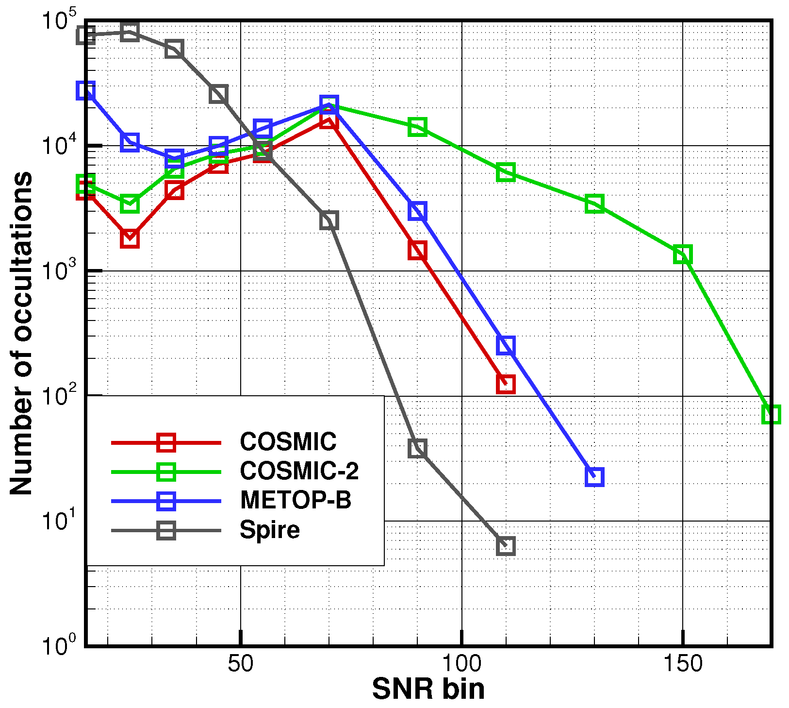
For COSMIC, we selected 24 days of the year 2008 (1st and 15th day of each month) for a total of 61,905 events (GPS only). For COSMIC-2, we selected 24 days of the year 2020 (1st and 15th day of each month) for a total of 107,173 events: 69,657 GPS and 37,518 GLONASS events. For METOP-B, we selected the whole year 2020, for a total of 196,158 events (GPS only). For Spire, we selected 24 days (1st and 15th days of each month) of the year 2020 and, additionally, 8 days of 2021 (1st, 8th, 15th, and 22nd day of June and July), for a total of 282,824 events: 113,039 GPS, 77,821 GLONASS, 83,707 Galileo, and 8276 QZSS events. The additional days were initially checked to compare their quality with the other periods. In fact, the overall quality of Spire data proved to be homogeneous. The occultation percentage in the SNR bins is shown in Figure 1.
3.2. COSMIC
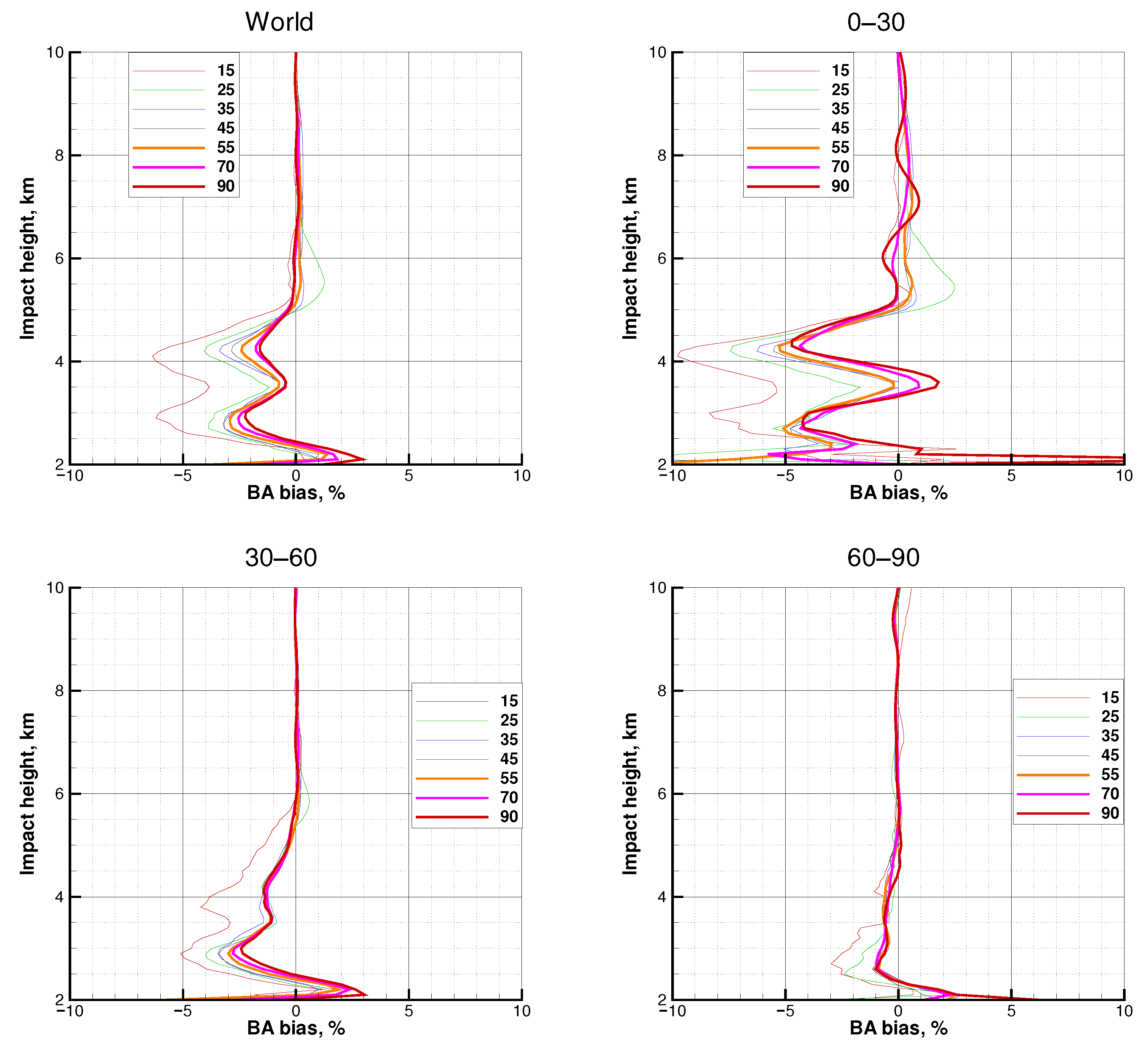
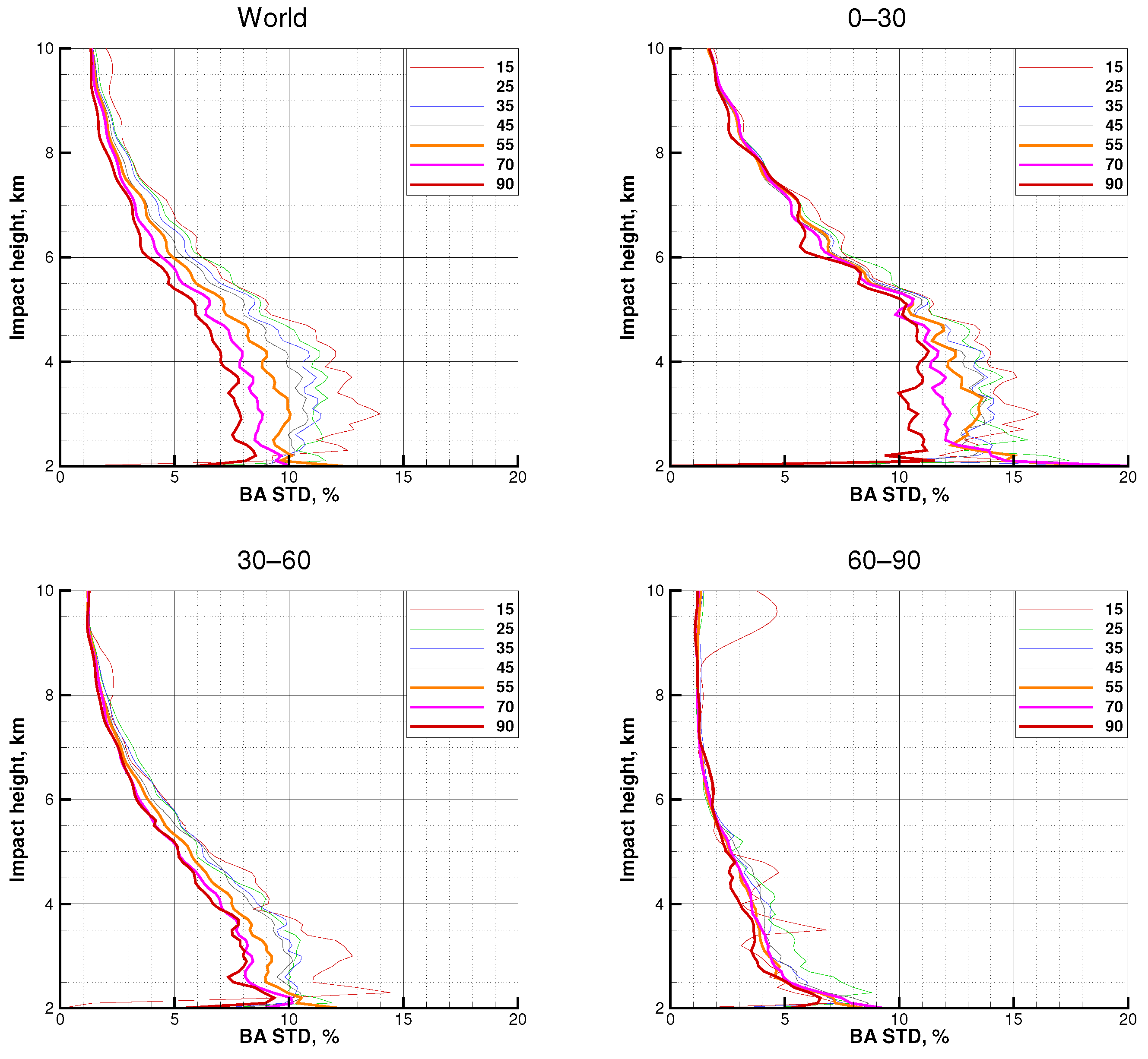
Figure 2, Figure 3 and Figure 4 show the bias, the STD, and the penetration for the COSMIC data as functions of the statically normalized SNR. The altitude is given above the Mean Sea Level (MSL), similar to [18]. Given the deviation of the bending angles for a specific mission from that evaluated for the background model, the bias is evaluated as , where the angular brackets denote the averaging of the ensemble of realizations. The STD is then evaluated as . The lowest SNR value of 15 belongs to the distribution tail, so the corresponding bias, STD, and penetration are unstable. The results indicate that the dynamically normalized SNR is a good estimator of data quality. The negative bias in the tropics and middle latitudes decreases in its absolute value with increasing SNR. The STD in these latitude bands also shows a significant decrease. In the polar latitudes, the dependence of STD on SNR is weaker.
In the framework of the model of the additive complex white noise, which we assume in this study, the noise in SNR translates to the phase noise. The propagation of such noise in the wave–optical retrieval chain was studied by [45], and it was shown that it is mostly the phase noise that influences the retrieval.
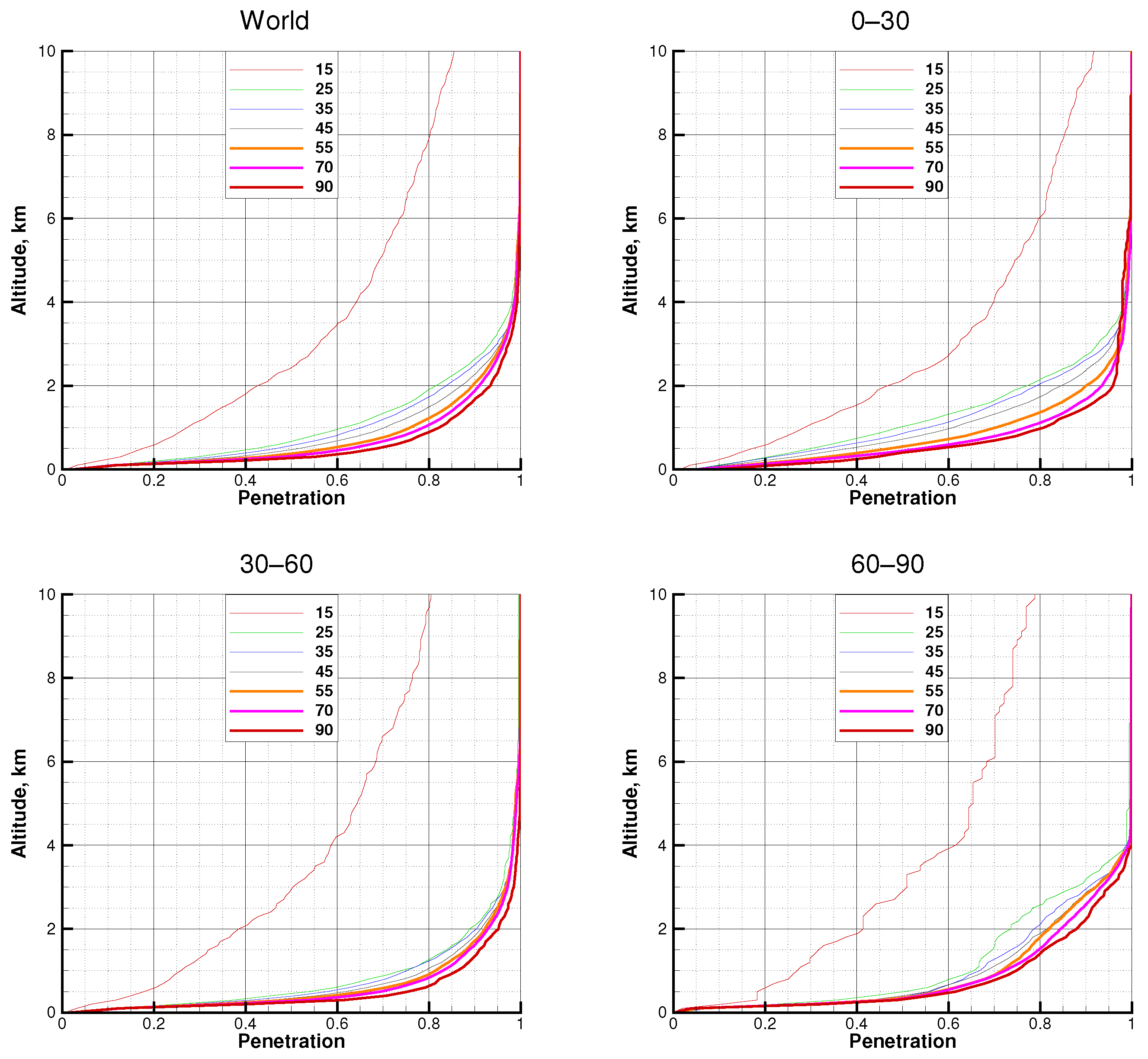
The penetration, defined as a fraction of valid refractivity points, indicates a steady improvement for increasing SNR. The penetration in the polar latitudes looks worse for all SNR bins, but this is the effect of the topography of the thick polar ice sheets.
3.3. COSMIC-2
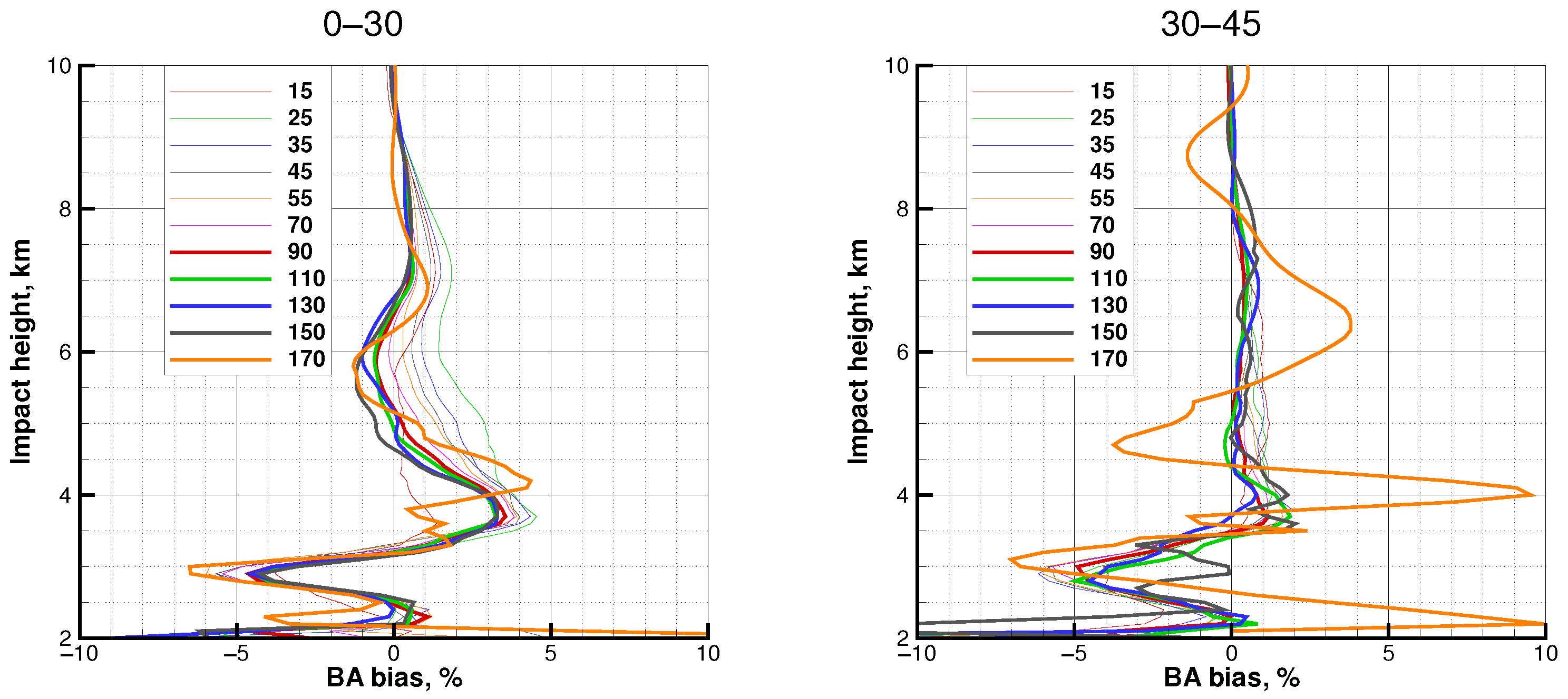
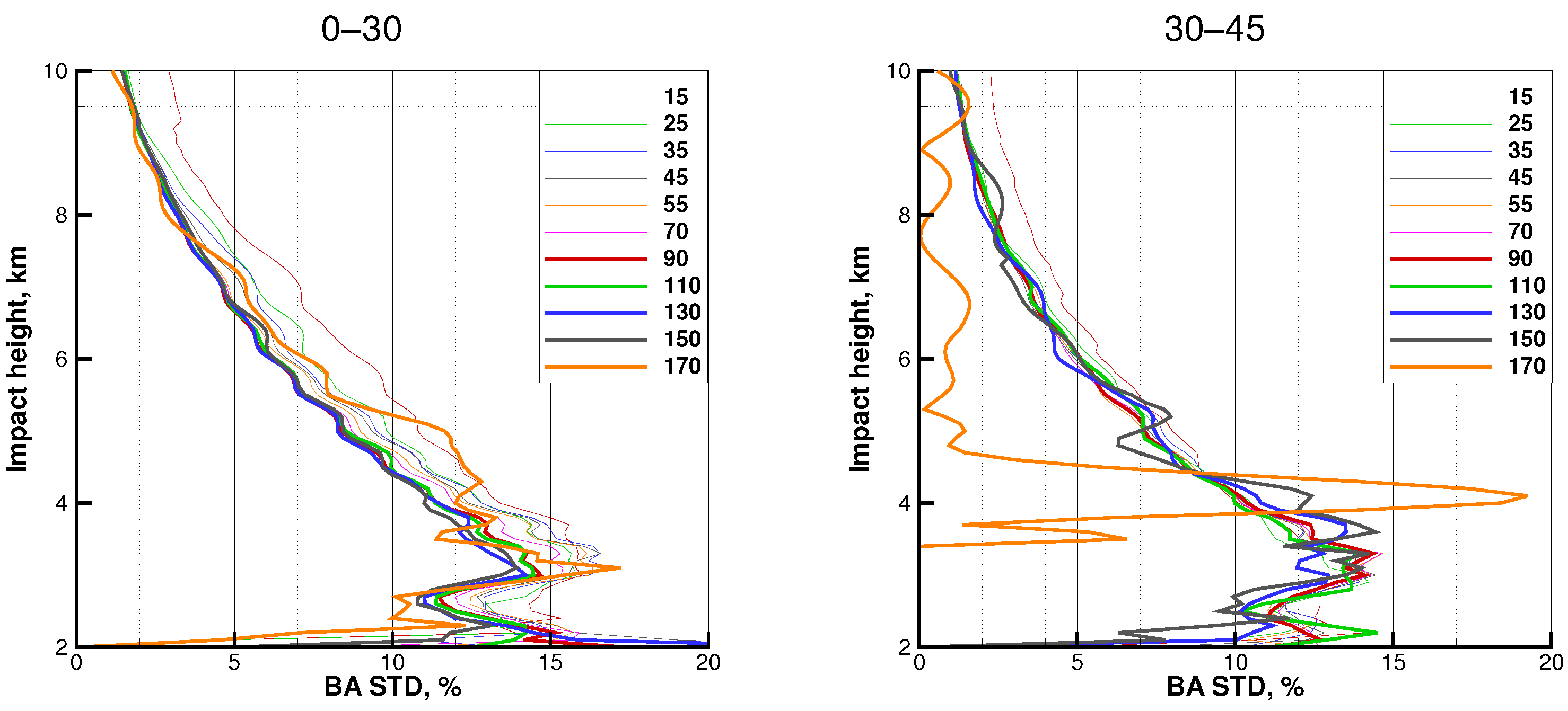
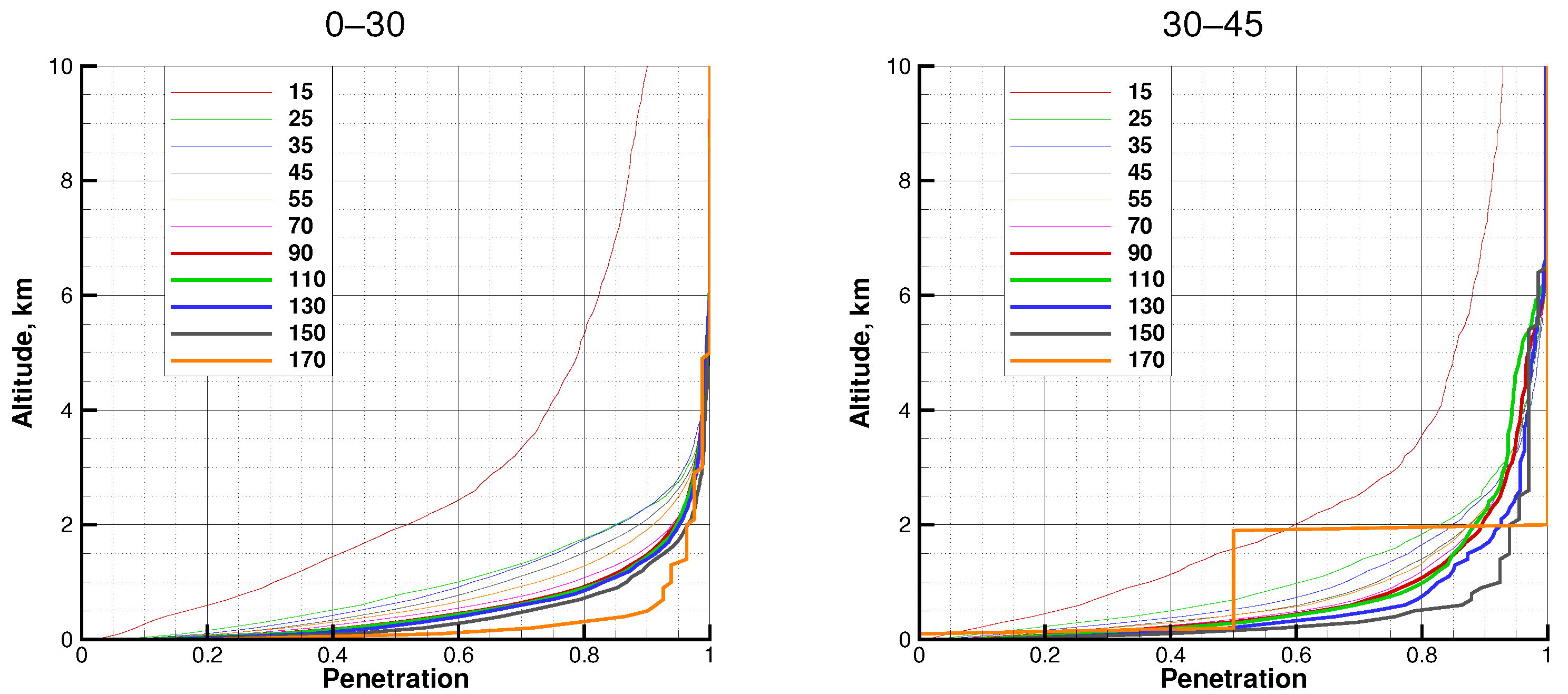
Figure 5, Figure 6 and Figure 7 show the bias, the STD, and the penetration for the COSMIC-2 data as functions of the dynamically normalized SNR. We only show tropics (0–30) and middle latitudes (30–45), because COSMIC-2 has very few profiles poleward of 45 degrees. For the bias, the general tendency is that its absolute value decreases with increasing SNR, which holds both for the positive and negative bias. The STD decreases with increasing SNR, although this dependence is less pronounced than for COSMIC. The penetration improves with increasing SNR, except for the polar region. The unstable behavior of the curves for SNR = 170 is explained by a low sample size.
3.4. Spire
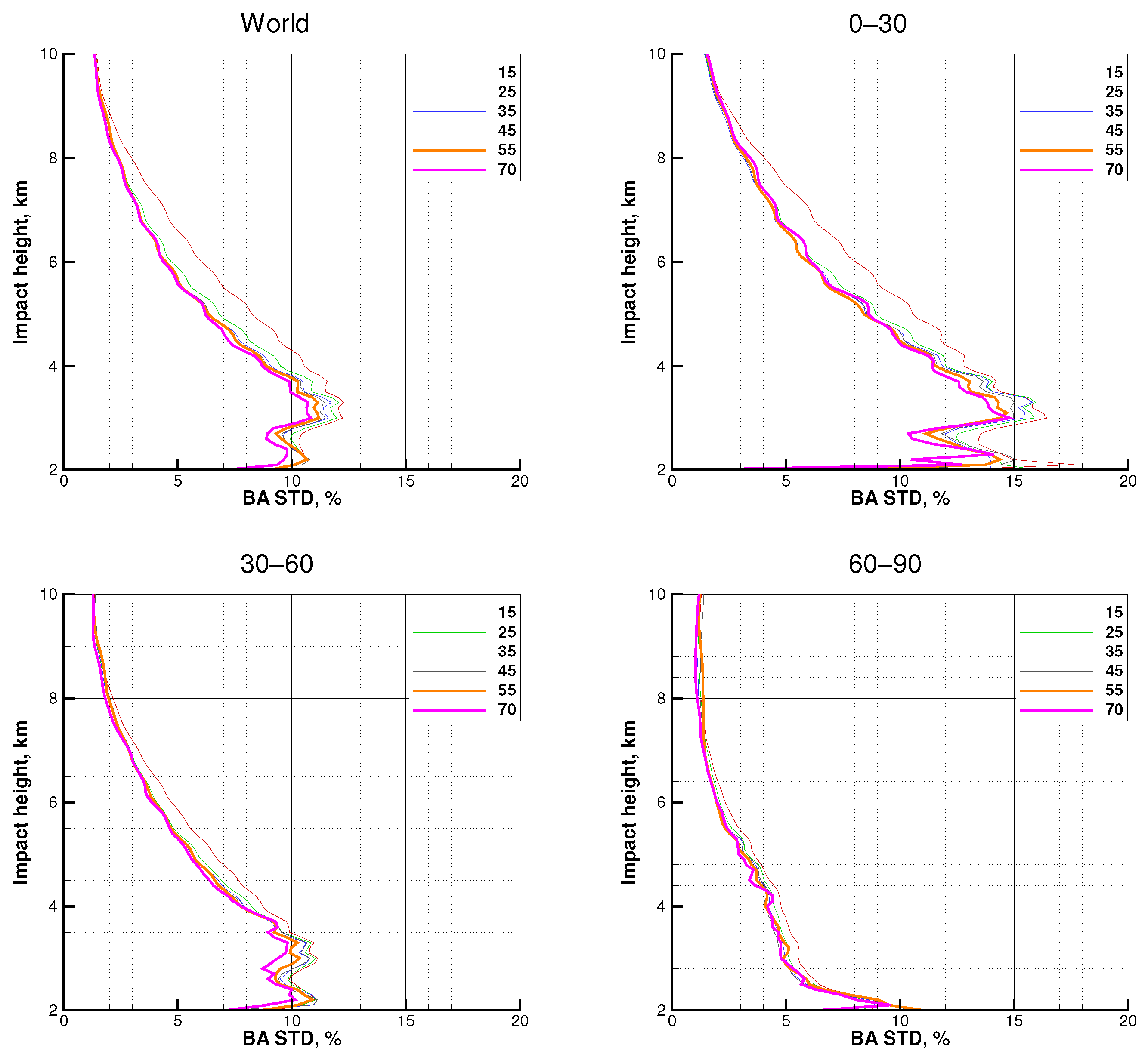
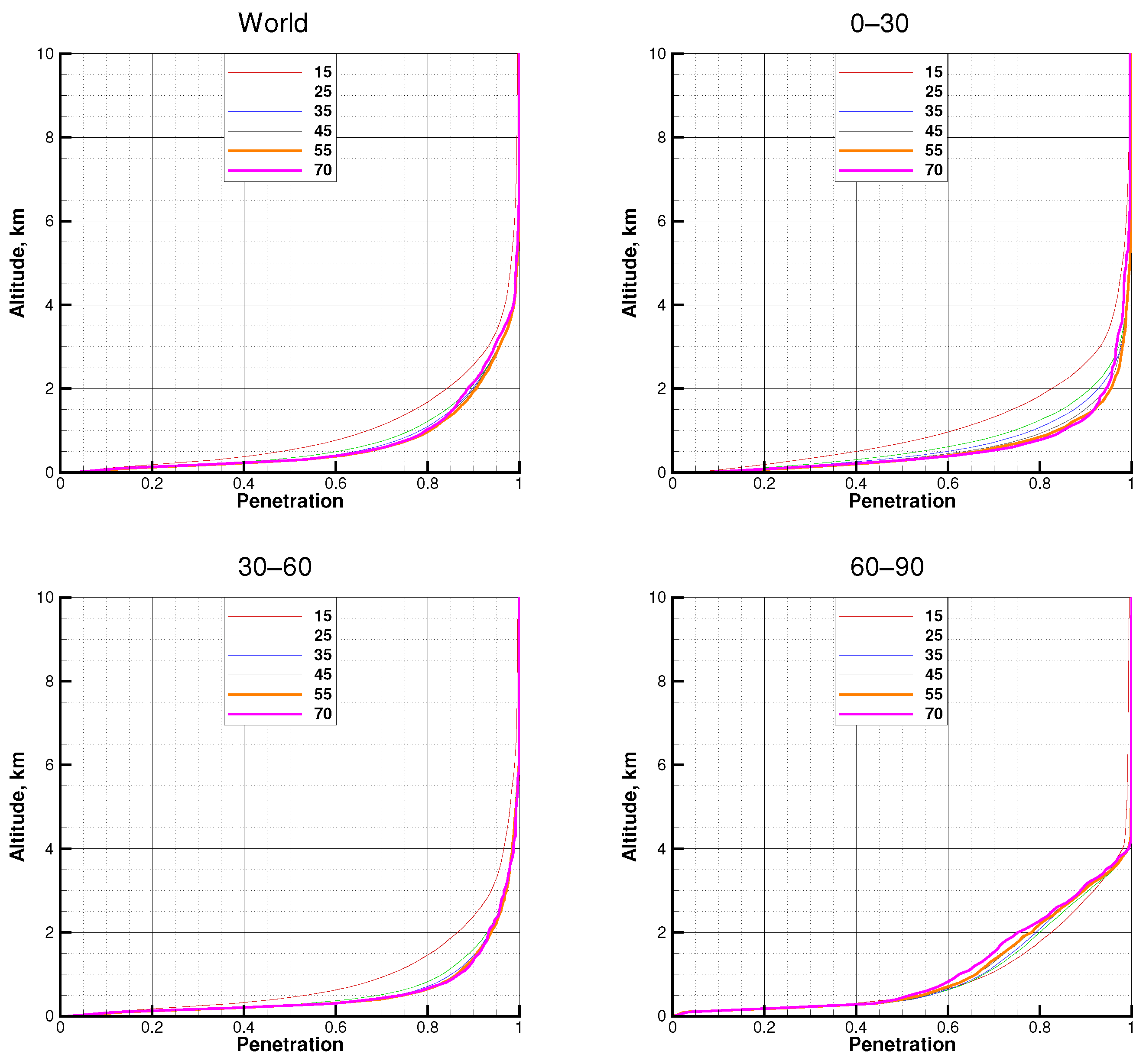
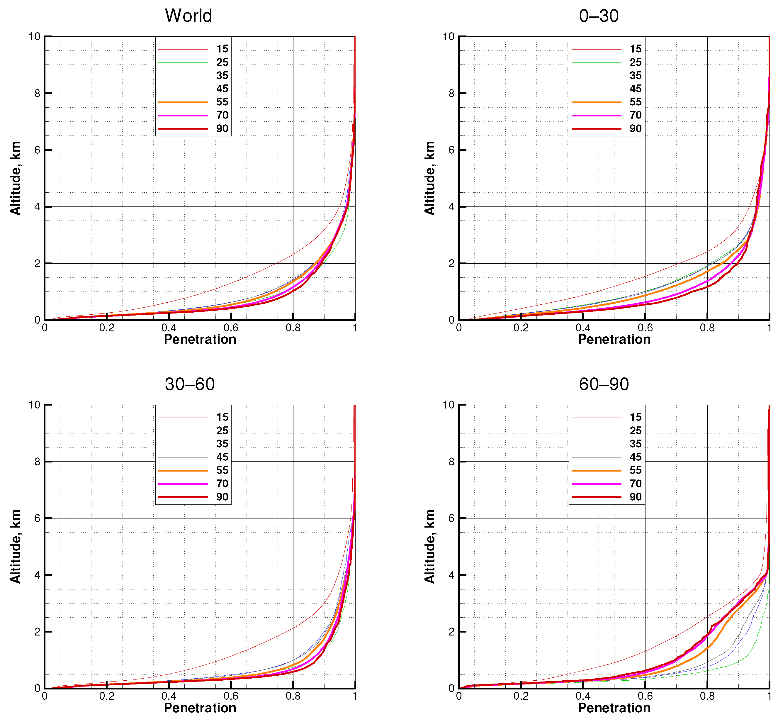
Figure 8, Figure 9 and Figure 10 show the bias, the STD, and the penetration for the Spire data as functions of the dynamically normalized SNR. The most characteristic feature of Spire data is the saturation at a relatively low SNR value. All differences become quite small above 25, and the bias saturates at an SNR of about 45, while the STD saturates at an SNR of about 35. The penetration in the tropics keeps enhancing with increasing SNR, while in the middle latitudes, it saturates at an SNR of about 55, and in the polar latitudes, it may be considered independent of the SNR.
3.5. METOP-B
Figure 11, Figure 12 and Figure 13 show the bias, the STD, and the penetration for the METOP-B data as functions of the dynamically normalized SNR. Due to the tracking strategy used in the METOP-B instrument, shadow zone measurements can only be used for setting RO events. Therefore, all the statistical results for METOP-B with a dynamically normalized SNR are exclusively based on setting events. The absolute value of the bias decreases with increasing SNR and saturates for SNR = 55. STD indicates a weak dependence on the SNR. It is most visible in the tropics, where it slightly decreases with an increasing SNR. The penetration improves with an increasing SNR. The strongest dependence of the penetration on the SNR is observed in the tropics.
3.6. All the Missions, SNR = 70
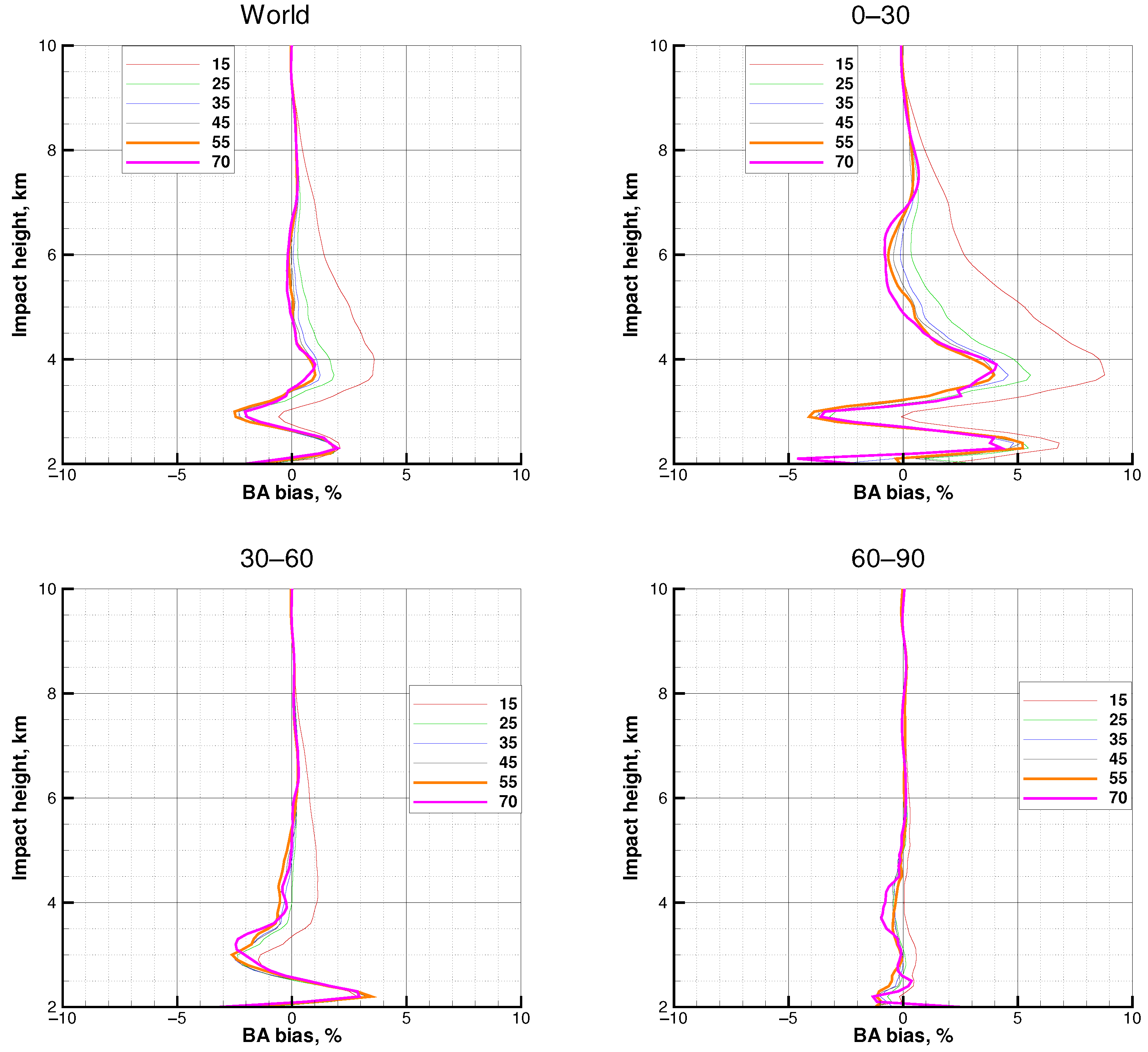
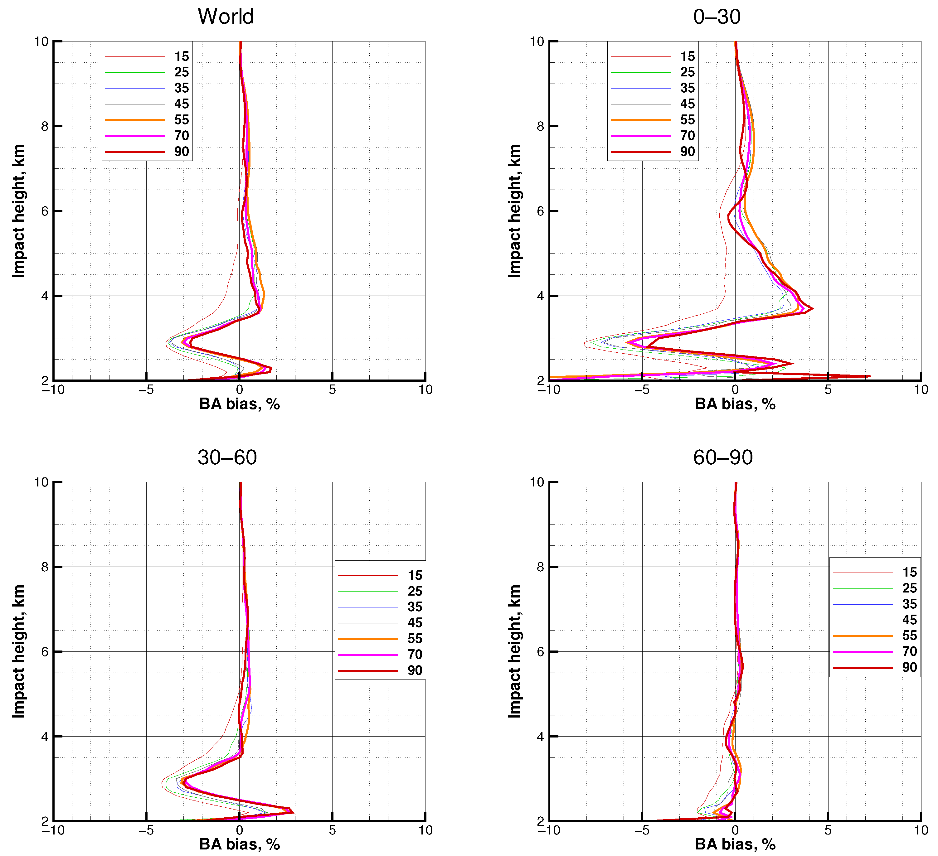
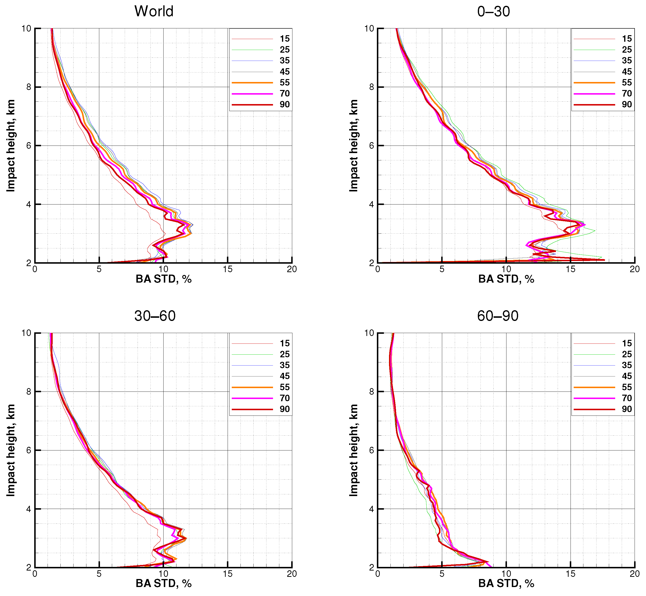
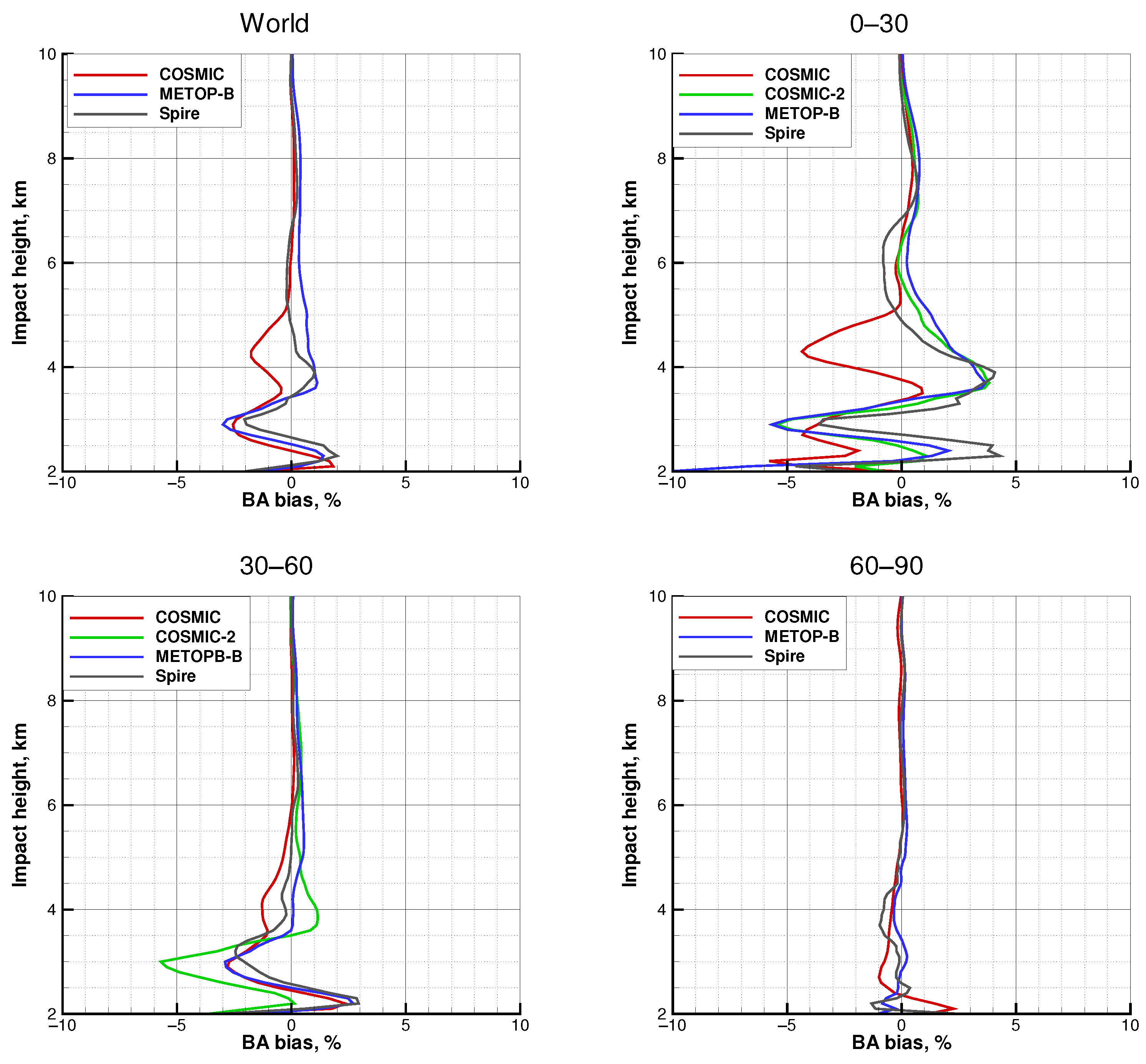
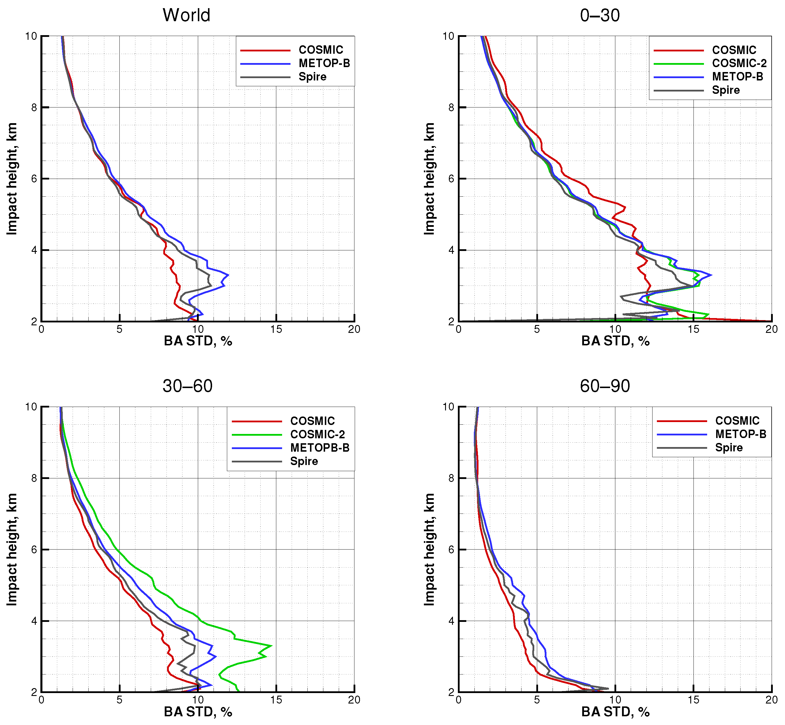
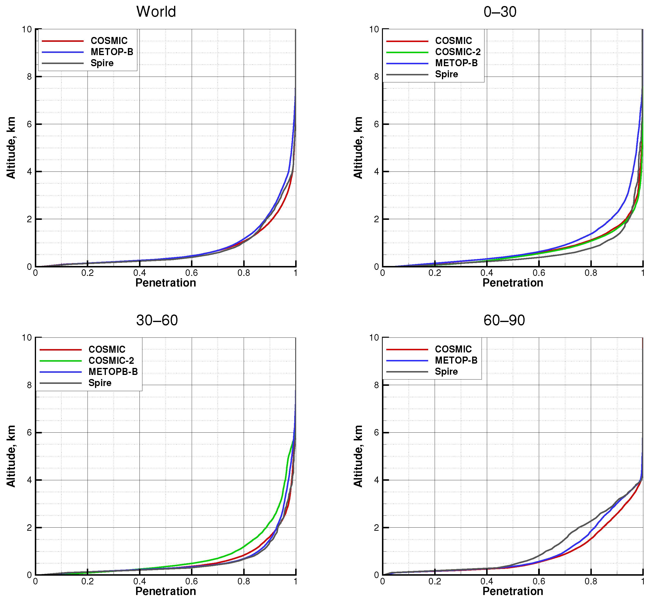
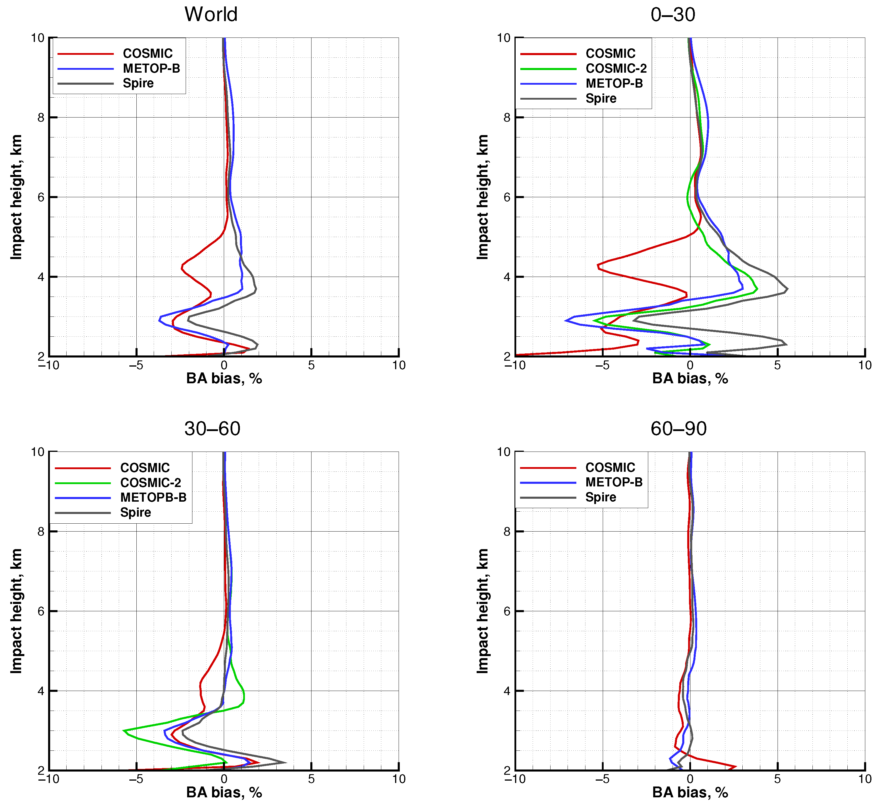
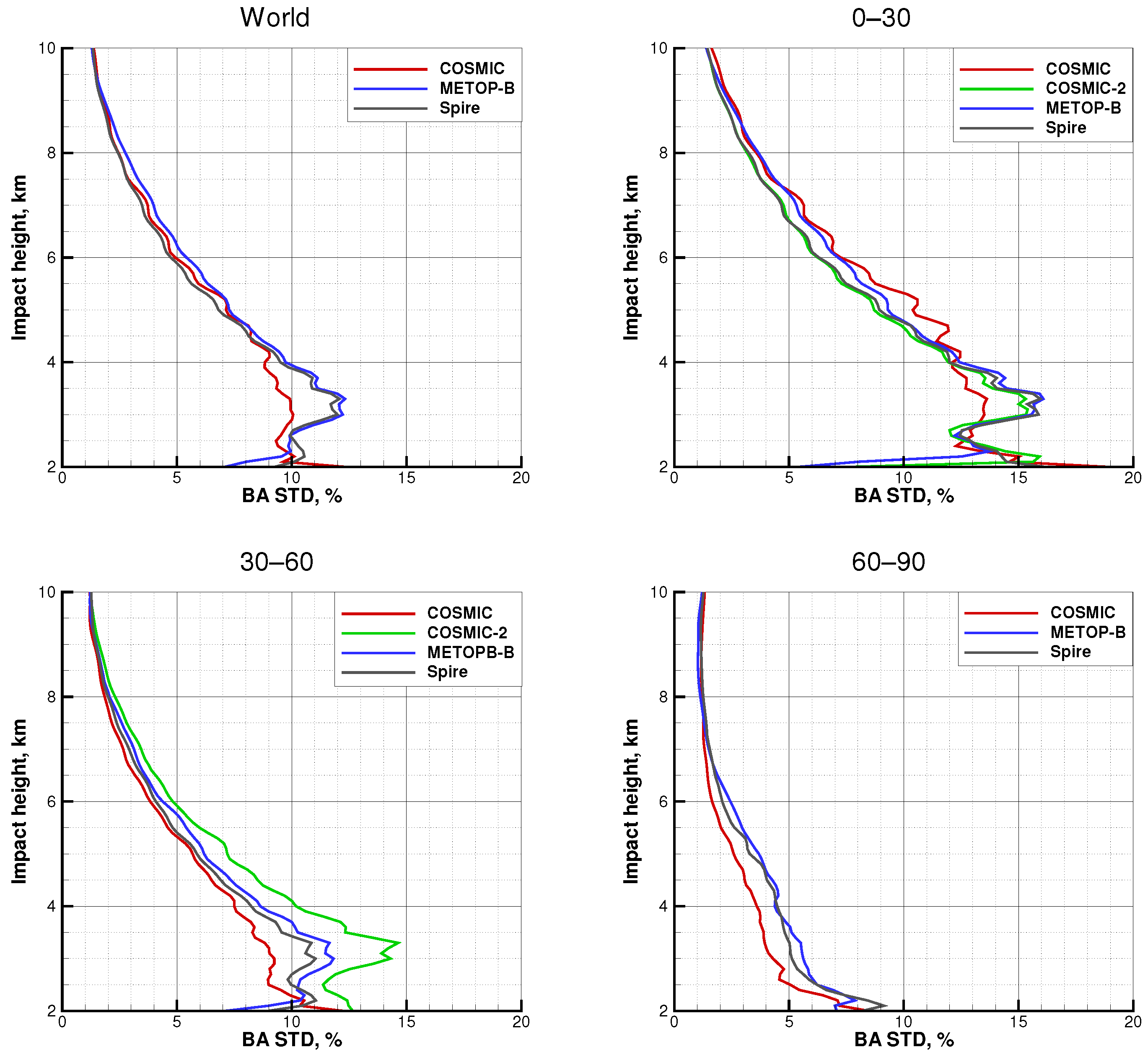
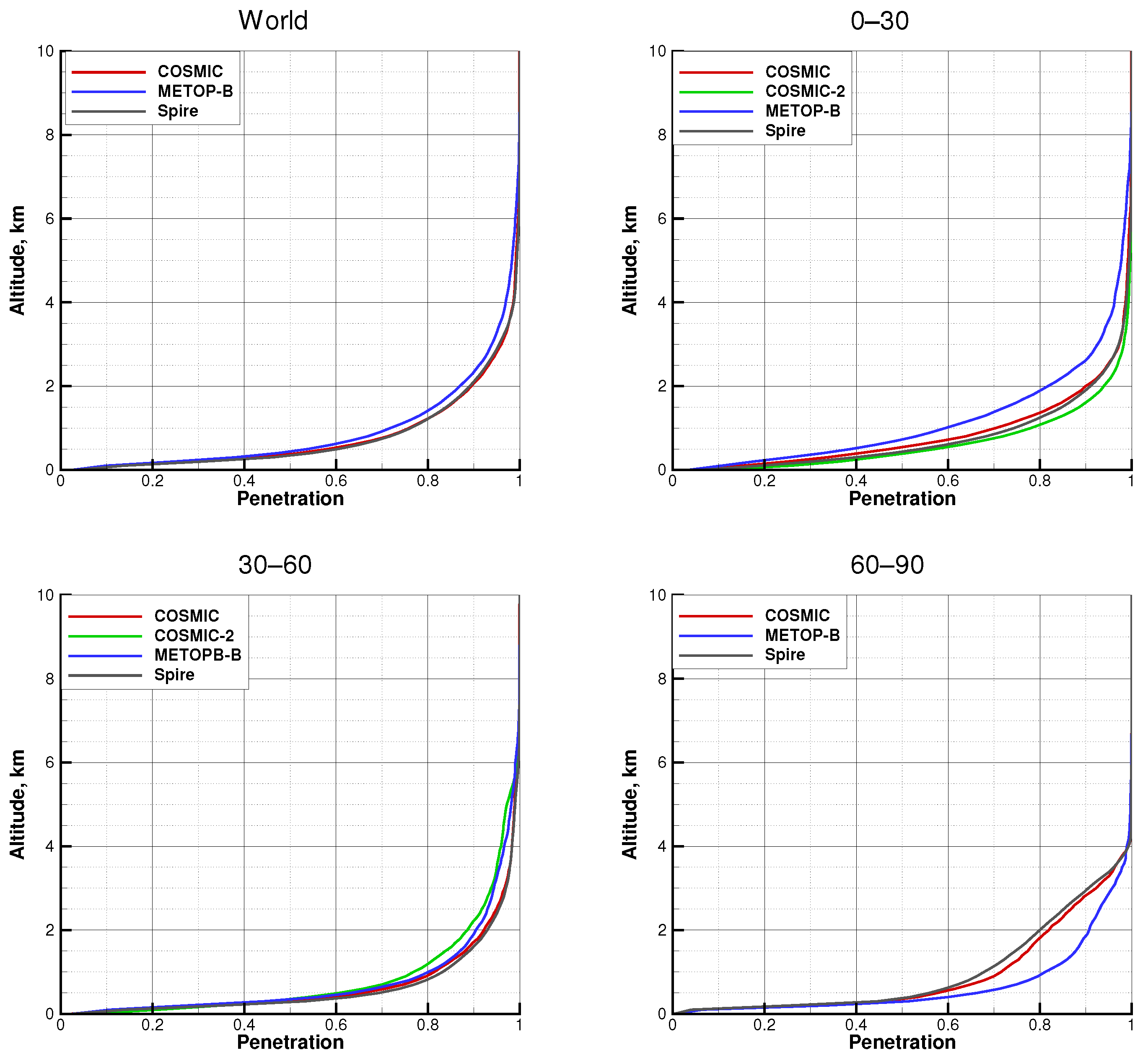
It is interesting to compare different missions for the same normalized SNR. We choose the SNR value of 70, as the highest value covered by all the missions. An SNR of 70 is the highest capability for Spire, but a middle value for COSMIC-2. Figure 14, Figure 15 and Figure 16 show the bias, STD, and penetration for an SNR of 70, for all the missions, for the dynamic normalization. COSMIC-2 is not included in the world statistics due its specific latitudinal distribution.
The bias patterns in the tropics for COSMIC-2, METOP-B, and Spire move closer to each other compared to the static normalization. There is, however, a significant difference between these missions and COSMIC. This is explained by the fact that the quality of the background GFS field in 2008 was not as good as in 2020.
In the comparison of the STD, it must be taken into account that COSMIC-2 has a special distribution of occultation locations, covering mostly the tropics and partly middle latitudes. Therefore, the STD should be compared in the tropics. Here, COSMIC-2 is close to METOP-B. For the impact height range 4–7 km and below 2.8 km, Spire is slightly better than the other missions. Between 2.8 and 4 km, COSMIC indicates the lowest STD. For the middle and polar latitudes, where COSMIC-2 should be excluded from the comparison, COSMIC indicates the best results. However, for the comparison over the globe, COSMIC indicates the lowest STD for the height range 2.5–4.2 km, and otherwise, COSMIC, METOP-B, and Spire are very close to each other.
In the tropics, the COSMIC and COSMIC-2 curves are nearly identical. METOP-B indicates worse penetration, while Spire shows a better penetration. The good penetration of Spire data was noticed independently by [28]. In the middle latitudes, COSMIC, METOP-B, and Spire demonstrate nearly identical penetration. Both static and dynamic normalizations show consistent results. This means that either of them can be used for inter-system comparison.
3.7. All the Missions, Median SNR
One more comparison is made for values of SNR that characterize the average capability of each mission. We determine each mission’s median SNRs, as shown in Table 1.
4. Discussion
The amplitude of RO signals decreases for lower ray perigee points due to the regular refraction. Upon this average decay, amplitude scintillations due to the complicated structure of the troposphere may be superimposed. In particular, thin humidity layers, which are typical, e.g., for the marine Planetary Boundary Layer (PBL), result in sharp spikes of the BA profile. Recovering such spikes requires measuring weak RO signals deep below the planet limb. This indicates that any additive noise imposes a restriction upon the lowest recoverable point of a profile. Our study indicates that a higher SNR improves the penetration. This effect is especially visible in the tropics, where the structure of RO signals is most complicated.
The bias in RO observation is difficult to understand because it has multiple components with different signs caused by different mechanisms [13,46,47,48]. Here, the bias patterns are similar for COSMIC-2, METOP-B, and Spire. The bias pattern for COSMIC differs significantly. Presumably, this is because these older data had to be evaluated with respect to GFS reference data from the year 2008, which had a lower resolution, height range, and accuracy as compared to GFS data for the years 2020 and 2021. The tropical bias of Spire below 3 km is shifted toward more positive values compared with other missions.
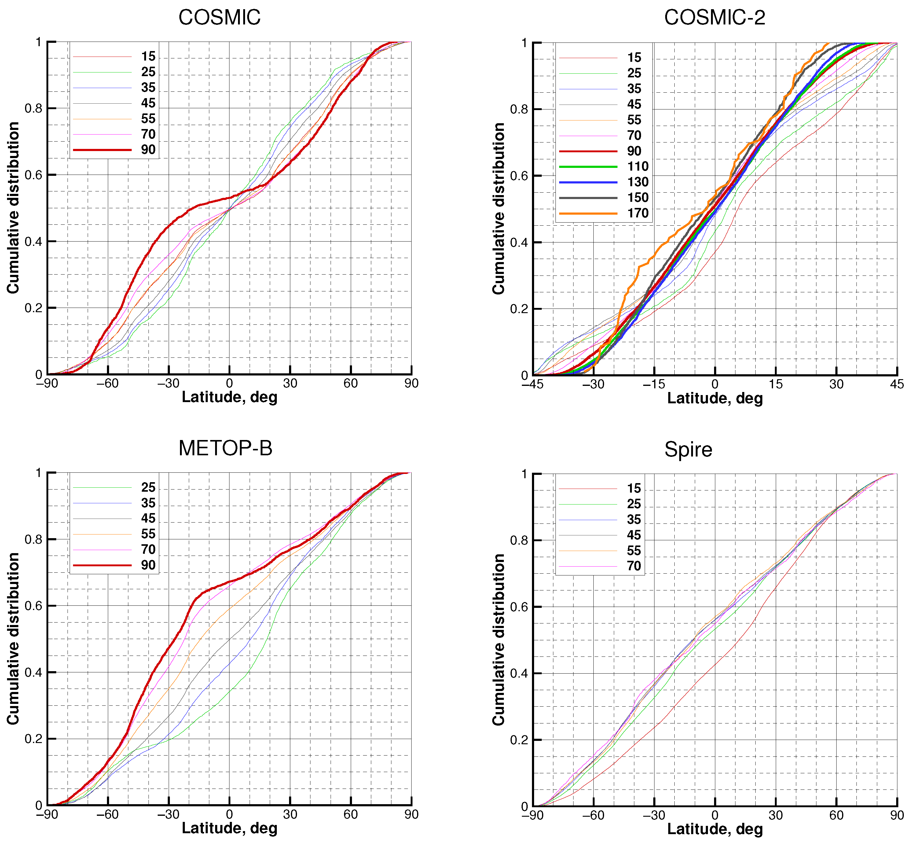
As regards the dependence of the bias on the SNR, the differences between missions are explained by the different dependence of their latitudinal distributions on the SNR, as shown in Figure 20. For Spire data, the latitudinal distribution indicates a very weak dependence on SNR, except the lowest SNR of 15. Therefore, here, we can see the best approximation to the “true” dependence of the statistics on the SNR. It indicates a tendency to saturation at some SNR level. The distribution also allows us to explain the somewhat unexpected behavior of COSMIC bias, which becomes more positive and strongly decreases by its absolute value with increasing SNR: for a higher SNR, a smaller fraction of COSMIC events falls into the central part of the tropical latitude band, where the negative bias is the biggest.
A study of the dependence of the COSMIC-2 inversion on the non-normalized SNR was performed by Ho et al. [19]. The occultations are divided into five groups: 0–500, 500–1000, 1000–1500, 1500–2000, and >2000 V/V. For these groups, the penetration in the tropics defined the occultation number fraction of 0.8, changing from 1.2–1.3 to 0.3–0.4 km. This is in qualitative agreement with our results indicating a steady improvement of the penetration with increasing SNR. It is difficult, however, to compare these results quantitatively, because they depend on the cut-off criteria, which involve a trade-off between a better penetration and worse STD. However, for METOP-B, the average penetration, without the evaluation of its dependence on SNR, is much worse: 3.3–4.4 km. In our study, the difference in the penetration between METOP-B and COSMIC is not that drastic. In the tropics, the METOP-B penetration is 1.2–1.9 km versus 0.5–1.7 km for COSMIC-2. In Schreiner et al. [18], we can also see a significant scatter of penetration depth estimates for different missions.
The mean fractional refractivity difference and standard deviation from the surface to 5 km altitude for the five SNR groups are estimated in [49] from a small sample (from 199 to 865 occultations), and it is impossible to see any clear dependence. Studies based on the three-cornered hat method [21,33] indicate that the error characteristics of COSMIC and COSMIC-2 are close to each other, which is consistent with our results.
5. Conclusions
In this study, we evaluated the statistics of four RO missions: COSMIC, COSMIC-2, METOP-B, and Spire. We used GFS analyses as the reference data. Our study was based on our previous work [32], in which we evaluated the statistical distributions of the NF for these missions. The central idea of this study is that the SNR expressed in V/V is evaluated by the receiver with respect to some intrinsic noise level and does not take into account different actual NF values. The NF depends on the mission and on the GNSS. We introduced two different definitions of the normalized SNR. The statically normalized SNR is the ratio of the average SNR in the 60–80 km range and the most probable NF value. The dynamically normalized SNR is the ratio of the average SNR in the 60–80 km range and the dynamic NF value for each specific occultation. The dynamic NF is evaluated by averaging the SNR in the shadow zone of each individual profile. This study utilizes the dynamic normalization. The leading idea is that the use of the normalized SNR makes different missions more comparable to each other.
We show that increasing the SNR improves the penetration of the radio occultation profiles, in agreement with previous studies. The effect of the SNR on the bending angle STD is mixed, with some missions showing a decrease of STD with increasing SNR in certain latitude bands and others showing little dependence of STD on the SNR. The STD in most cases indicates saturation: it is large for a small SNR, but for a moderately large SNR, its dependence becomes weaker.
We evaluated the dependence of the latitudinal distribution of the occultations of the four missions. We found for Spire that the latitudinal distribution is nearly independent of the SNR. This correlates with the fact that the Spire data indicate the saturation effect very well. For COSMIC data, on the contrary, for a higher SNR, a smaller fraction of events falls into the central part of the tropical latitude band. This results in a stronger dependence of the STD on the SNR.
The bending angle STDs appear to be close to each other for all missions despite quite strong differences in the normalized SNR (Table 1) and even stronger differences between the nominal SNRs [32]. We can conclude that higher SNR values do not necessarily result in a proportionally higher statistical quality of the RO profiles, if the SNR is above a certain threshold. On the other hand, the high-SNR RO data are believed to be valuable for scientific studies of super-refraction and the boundary layer.
The bias in RO retrievals is a complicated effect caused by multiple mechanisms, and its dependence on the SNR is not very obvious. As follows from [47], a higher SNR shifts the bias in the negative direction. This effect is observed for COSMIC-2 in the tropics, where it indicates the strongest dependence on the SNR. For COSMIC, we observe that the bias is shifted in the positive direction for an increasing normalized SNR. However, this is explained by the specific dependence of the COSMIC distribution on the normalized SNR.
Author Contributions
Conceptualization, M.G., V.I., and C.R.; methodology, M.G.; software, M.G. All authors have read and agreed to the published version of the manuscript.
Funding
The work of M.G. was supported by Russian Foundation for Basic Research, grant No. 20-05-00189 A.
Data Availability Statement
The COSMIC, METOP, and COSMIC2 data used in this study are freely available from the CDAAC Web-site. The Spire data used in this study are only distributed on a commercial basis or provided in the framework of special agreements.
Acknowledgments
The authors acknowledge Taiwan’s National Space Organization (NSPO) and the University Corporation for Atmospheric Research (UCAR) for providing the COSMIC and COSMIC-2 Data.
Conflicts of Interest
The authors declare no conflict of interest.
Abbreviations
The following abbreviations are used in this manuscript:
| BA | Bending Angle |
| BS | Badness Score |
| CDAAC | COSMIC Data Analysis and Archive Center |
| COSMIC | Constellation Observing System for Meteorology, Ionosphere, and Climate |
| CT2 | Canonical Transform |
| GFS | Global Forecast System |
| GNSS | Global Navigation Satellite Signal System |
| GO | Geometric Optics |
| LEO | Low Earth Orbiter |
| MSISE | Mass-Spectrometer-Incoherent-Scatter model Extended |
| MSL | Mean Sea Level |
| NCEP | of National Centers for Environmental Prediction |
| NF | Noise Floor |
| NWP | Numerical Weather Prediction |
| PBL | Planetary Boundary Layer |
| QC | Quality Control |
| RO | Radio Occultation |
| SNR | Signal-to-Noise Ratio |
References
- Von Engeln, A.; Nedoluha, G.; Kirchengast, G.; Bühler, S. One-dimensional variational (1-D Var) retrieval of temperature, water vapor, and a reference pressure from radio occultation measurements: A sensitivity analysis. J. Geophys. Res. 2003, 108, 4337. [Google Scholar] [CrossRef]
- Healy, S.B.; Thépaut, J.N. Assimilation experiments with CHAMP GPS radio occultation measurements. Quart. J. Roy. Meteor. Soc. 2006, 132, 605–623. [Google Scholar] [CrossRef]
- Healy, S.B.; Eyre, J.R.; Hamrud, M.; Thépaut, J.N. Assimilating GPS radio occultation measurements with two-dimensional bending angle observation operators. Quart. J. Roy. Meteor. Soc. 2007, 133, 1213–1227. [Google Scholar] [CrossRef]
- Cucurull, L.; Derber, J.C.; Purser, R.J. A bending angle forward operator for global positioning system radio occultation measurements. J. Geophys. Res. 2013, 118, 14–28. [Google Scholar] [CrossRef]
- Burrows, C.P.; Healy, S.B.; Culverwell, I.D. Improving the bias characteristics of the ROPP refractivity and bending angle operators. Atmos. Meas. Tech. 2014, 7, 3445–3458. [Google Scholar] [CrossRef] [Green Version]
- Gorbunov, M.; Stefanescu, R.; Irisov, V.; Zupanski, D. Variational Assimilation of Radio Occultation Observations into Numerical Weather Prediction Models: Equations, Strategies, and Algorithms. Remote Sens. 2019, 11, 2886. [Google Scholar] [CrossRef] [Green Version]
- Syndergaard, S. On the ionosphere calibration in GPS radio occultation measurements. Radio Sci. 2000, 35, 865–883. [Google Scholar] [CrossRef]
- Gorbunov, M.E. Ionospheric correction and statistical optimization of radio occultation data. Radio Sci. 2002, 37, 17-1–17-9. [Google Scholar] [CrossRef] [Green Version]
- Sokolovskiy, S.; Schreiner, W.; Rocken, C.; Hunt, D. Optimal Noise Filtering for the Ionospheric Correction of GPS Radio Occultation Signals. J. Atmos. Ocean. Technol. 2009, 26, 1398–1403. [Google Scholar] [CrossRef]
- Angling, M.J.; Elvidge, S.; Healy, S.B. Improved model for correcting the ionospheric impact on bending angle in radio occultation measurements. Atmos. Meas. Tech. 2018, 11, 2213–2224. [Google Scholar] [CrossRef] [Green Version]
- Danzer, J.; Haas, S.J.; Schwaerz, M.; Kirchengast, G. Performance of the Ionospheric Kappa-Correction of Radio Occultation Profiles Under Diverse Ionization and Solar Activity Conditions. Earth Space Sci. 2021, 8, e2020EA001581. [Google Scholar] [CrossRef] [PubMed]
- Aragon-Angel, A.; Rovira-Garcia, A.; Arcediano-Garrido, E.; Ibáñez-Segura, D. Galileo Ionospheric Correction Algorithm Integration into the Open-Source GNSS Laboratory Tool Suite (gLAB). Remote Sens. 2021, 13, 191. [Google Scholar] [CrossRef]
- Sokolovskiy, S.; Schreiner, W.; Zeng, Z.; Hunt, D.; Lin, Y.C.; Kuo, Y.H. Observation, analysis, and modeling of deep radio occultation signals: Effects of tropospheric ducts and interfering signals. Radio Sci. 2014, 49, 954–970. [Google Scholar] [CrossRef]
- Bonnedal, M.; Christensen, J.; Carlström, A.; Berg, A. Metop-GRAS in-orbit instrument performance. GPS Solut. 2010, 14, 109–120. [Google Scholar] [CrossRef]
- Schreiner, W.; Sokolovskiy, S.; Hunt, D.; Rocken, C.; Kuo, Y.H. Analysis of GPS radio occultation data from the FORMOSAT-3/COSMIC and Metop/GRAS missions at CDAAC. Atmos. Meas. Tech. 2011, 4, 2255–2272. [Google Scholar] [CrossRef] [Green Version]
- Xu, X.; Zou, X. Comparison of MetOp-A/-B GRAS radio occultation data processed by CDAAC and ROM. GPS Solut. 2020, 24. [Google Scholar] [CrossRef]
- Sokolovskiy, S.; Schreiner, W.; Weiss, J.; Zeng, Z.; Hunt, D.; Braun, J. Initial Assessment of COSMIC-2 Data in the Lower Troposphere. In Proceedings of the Joint 6th ROM SAF Data User Workshop and 7th IROWG Workshop, Konventum, Elsinore, Denmark, 19–25 September 2019. [Google Scholar]
- Schreiner, W.S.; Weiss, J.; Anthes, R.A.; Braun, J.J.; Chu, V.; Fong, J.; Hunt, D.; Kuo, Y.H.; Meehan, T.K.; Xia-Serafino, W.; et al. COSMIC-2 Radio Occultation Constellation: First Results. Geophys. Res. Lett. 2020, 47, e2019GL086841. [Google Scholar] [CrossRef]
- Ho, S.P.; Zhou, X.; Shao, X.; Zhang, B.; Adhikari, L.; Kireev, S.; He, Y.; Yoe, J.G.; Xia-Serafino, W.; Lynch, E. Initial Assessment of the COSMIC-2/FORMOSAT-7 Neutral Atmosphere Data Quality in NESDIS/STAR Using In Situ and Satellite Data. Remote Sens. 2020, 12, 4099. [Google Scholar] [CrossRef]
- Lin, C.Y.; Lin, C.C.H.; Liu, J.Y.; Rajesh, P.K.; Matsuo, T.; Chou, M.Y.; Tsai, H.F.; Yeh, W.H. The Early Results and Validation of FORMOSAT-7/COSMIC-2 Space Weather Products: Global Ionospheric Specification and Ne-Aided Abel Electron Density Profile. J. Geophys. Res. Space Phys. 2020, 125, e2020JA028028. [Google Scholar] [CrossRef]
- Rieckh, T.; Sjoberg, J.P.; Anthes, R.A. The Three-Cornered Hat Method for Estimating Error Variances of Three or More Atmospheric Datasets. Part II: Evaluating Radio Occultation and Radiosonde Observations, Global Model Forecasts, and Reanalyses. J. Atmos. Ocean. Technol. 2021, 38, 1777–1796. [Google Scholar] [CrossRef]
- Kursinski, E.R. Weather & Space Weather RO Data from PlanetiQ Commercial GNSS RO. In Proceedings of the Joint 6th ROM SAF Data User Workshop and 7th IROWG Workshop, Konventum, Elsinore, Denmark, 19–25 September 2019. [Google Scholar]
- Chang, H.; Lee, J.; Wang, Y.; Breitsch, B.; Morton, Y.J. Preliminary Assessment of CICERO Radio Occultation Performance by Comparing with COSMIC I Data. In Proceedings of the 33rd International Technical Meeting of the Satellite Division of The Institute of Navigation. Institute of Navigation, Manassas, VA, USA, 21–25 September 2020. [Google Scholar] [CrossRef]
- Irisov, V.; Duly, T.; Nguyen, V.; Masters, D.; Nogues-Correig, O.; Tan, L.; Yuasa, T.; Ector, D. Recent radio occultation profile results obtained from Spire CubeSat GNSS-RO constellation. In Proceedings of the AGU Fall Meeting, Washington, DC, USA, 10–14 December 2018. [Google Scholar]
- Irisov, V.; Ector, D.; Duly, T.; Nguyen, V.; Nogues-Correig, O.; Tan, L.; Yuasa, T. Atmospheric Radio Occultation Observation from Spire CubeSat Nanosatellites. In Proceedings of the AMS Annual Meeting, Austin, TX, USA, 7–11 January 2018. [Google Scholar]
- Gorbunov, M.; Koval, O.; Kirchengast, G. Kirkwood Distribution Function and its Applicationfor the Analysis of Radio Occultation Observations. In Proceedings of the Joint 6th ROM SAF User Workshop and 7th IROWG Workshop, EUMETSAT ROM SAF, Elsinore, Denmark, 19–25 September 2019. [Google Scholar]
- Irisov, V.; Nguyen, V.; Duly, T.; Nogues-Correig, O.; Tan, L.; Yuasa, T.; Masters, D.; Sikarin, R.; Gorbunov, M.; Rocken, C. Radio Occultation Observations and Processing from Spire’s CubeSat Constellation. In Proceedings of the Joint 6th ROM SAF User Workshop and 7th IROWG Workshop, EUMETSAT ROM SAF, Elsinore, Denmark, 19–25 September 2019. [Google Scholar]
- Bowler, N.E. An assessment of GNSS radio occultation data produced by Spire. Q. J. R. Meteorol. Soc. 2020, 146, 3772–3788. [Google Scholar] [CrossRef]
- Lonitz, K.; Marquardt, C.; Bowler, N.; Healy, S. Final Technical Note of Impact Assessment of Commercial GNSS-RO Data; ESA Contract Report 4000131086/20/NL/FF/a; European Centre for Medium Range Weather Forecasts: Reading, UK, 2021. [Google Scholar]
- Sokolovskiy, S.; Rocken, C.; Hunt, D.; Schreiner, W.; Johnson, J.; Masters, D.; Esterhuizen, S. GPS profiling of the lower troposphere from space: Inversion and demodulation of the open-loop radio occultation signals. Geophys. Res. Lett. 2006, 33, L14816. [Google Scholar] [CrossRef] [Green Version]
- Kuo, Y.H.; Wee, T.K.; Sokolovskiy, S.; Rocken, C.; Schreiner, W.; Hunt, D.; Anthes, R.A. Inversion and Error Estimation of GPS Radio Occultation Data. J. Meteorolog. Soc. Jpn. 2004, 82, 507–531. [Google Scholar] [CrossRef] [Green Version]
- Gorbunov, M.; Irisov, V.; Rocken, C. Noise Floor and Signal-to-Noise Ratio of Radio Occultation Observations: A Cross-Mission Statistical Comparison. Remote Sens. 2022, 14, 691. [Google Scholar] [CrossRef]
- Anthes, R.; Sjoberg, J.; Feng, X.; Syndergaard, S. Comparison of COSMIC and COSMIC-2 Radio Occultation Refractivity and Bending Angle Uncertainties in August 2006 and 2021. Atmosphere 2022, 13, 790. [Google Scholar] [CrossRef]
- Gorbunov, M.E.; Lauritsen, K.B. Analysis of wave fields by Fourier integral operators and its application for radio occultations. Radio Sci. 2004, 39, RS4010. [Google Scholar] [CrossRef]
- Gorbunov, M.E.; Lauritsen, K.B.; Rodin, A.; Tomassini, M.; Kornblueh, L. Analysis of the CHAMP experimental data on radio-occultation sounding of the Earth’s atmosphere. Izv. Atmos. Ocean. Phys. 2005, 41, 726–740. [Google Scholar]
- Gorbunov, M.E.; Lauritsen, K.B.; Rhodin, A.; Tomassini, M.; Kornblueh, L. Radio holographic filtering, error estimation, and quality control of radio occultation data. J. Geophys. Res. 2006, 111, D10105. [Google Scholar] [CrossRef] [Green Version]
- Hedin, A.E. Extension of MSIS thermosphere model into the middle and lower atmosphere. J. Geophys. Res. 1991, 96, 1159–1172. [Google Scholar] [CrossRef]
- Sokolovskiy, S.V. Modeling and inverting radio occultation signals in the moist troposphere. Radio Sci. 2001, 36, 441–458. [Google Scholar] [CrossRef] [Green Version]
- Gorbunov, M.E.; Sokolovskiy, S.V. Remote Sensing of Refractivity from Space for Global Observations of Atmospheric Parameters; Report 119; Max-Planck Institute for Meteorology: Hamburg, Germany, 1993; 58p. [Google Scholar]
- Gorbunov, M.E.; Gurvich, A.S.; Shmakov, A.V. Back-propagation and radio-holographic methods for investigation of sporadic ionospheric E-layers from Microlab-1 data. Int. J. Remote Sens. 2002, 23, 675–685. [Google Scholar] [CrossRef]
- Sokolovskiy, S.V.; Schreiner, W.; Rocken, C.; Hunt, D. Detection of high-altitude ionospheric irregularities with GPS/MET. Geophys. Res. Let. 2002, 29, 3-1–3-4. [Google Scholar] [CrossRef] [Green Version]
- Gorbunov, M.E.; Shmakov, A.V.; Leroy, S.S.; Lauritsen, K.B. COSMIC Radio Occultation Processing: Cross-center Comparison and Validation. J. Atmos. Ocean. Technol. 2011, 28, 737–751. [Google Scholar] [CrossRef]
- Kan, V.; Gorbunov, M.E.; Shmakov, A.V.; Sofieva, V.F. The Reconstruction of the Parameters of Internal Gravity Waves in the Atmosphere from Amplitude Fluctuations in the Radio Occultation Experiment. Izv. Atm. Ocean. Phys. 2020, 56, 435–447. [Google Scholar] [CrossRef]
- Kan, V.; Gorbunov, M.E.; Fedorova, O.V.; Sofieva, V.F. Latitudinal Distribution of the Parameters of Internal Gravity Waves in the Atmosphere Derived from Amplitude Fluctuations of Radio Occultation Signals. Izv. Atm. Ocean. Phys. 2020, 56, 564–575. [Google Scholar] [CrossRef]
- Gorbunov, M.E.; Kirchengast, G. Uncertainty propagation through wave optics retrieval of bending angles from GPS radio occultation: Theory and simulation results. Radio Sci. 2015, 50, 1086–1096. [Google Scholar] [CrossRef] [Green Version]
- Sokolovskiy, S.V. Effect of super refraction on inversions of radio occultation signals in the lower troposphere. Radio Sci. 2003, 38, 1058. [Google Scholar] [CrossRef] [Green Version]
- Sokolovskiy, S.; Rocken, C.; Schreiner, W.; Hunt, D. On the uncertainty of radio occultation inversions in the lower troposphere. J. Geophys. Res. 2010, 115, D22111. [Google Scholar] [CrossRef] [Green Version]
- Gorbunov, M.E.; Vorob’ev, V.V.; Lauritsen, K.B. Fluctuations of refractivity as a systematic error source in radio occultations. Radio Sci. 2015, 50, 656–669. [Google Scholar] [CrossRef]
- Ho, S.p.; Anthes, R.A.; Ao, C.O.; Healy, S.; Horanyi, A.; Hunt, D.; Mannucci, A.J.; Pedatella, N.; Randel, W.J.; Simmons, A.; et al. The COSMIC/FORMOSAT-3 Radio Occultation Mission after 12 Years: Accomplishments, Remaining Challenges, and Potential Impacts of COSMIC-2. Bull. Am. Meteorol. Soc. 2020, 101, E1107–E1136. [Google Scholar] [CrossRef] [Green Version]
Figure 1.
The number of occultations in the SNR bins.

Figure 2.
Statistical comparison of bending angles retrieved from RO observations with GFS analyses for different normalized SNRs. COSMIC, systematic difference, dynamic normalization. Upper left: world, upper right: tropics, lower left: middle latitudes, lower right: polar latitudes. All the latitude bins cover both North and South hemispheres.

Figure 3.
Similar to Figure 2. COSMIC, standard deviation.
Figure 3.
Similar to Figure 2. COSMIC, standard deviation.

Figure 4.
Similar to Figure 2. COSMIC, penetration.
Figure 4.
Similar to Figure 2. COSMIC, penetration.

Figure 5.
Similar to Figure 2. COSMIC-2, systematic difference. COSMIC-2 profiles are limited by degrees latitudes.
Figure 5.
Similar to Figure 2. COSMIC-2, systematic difference. COSMIC-2 profiles are limited by degrees latitudes.

Figure 6.
Similar to Figure 3. COSMIC-2, standard deviation.
Figure 6.
Similar to Figure 3. COSMIC-2, standard deviation.

Figure 7.
Similar to Figure 4. COSMIC-2, penetration.
Figure 7.
Similar to Figure 4. COSMIC-2, penetration.

Figure 8.
Similar to Figure 2. Spire, systematic difference.
Figure 8.
Similar to Figure 2. Spire, systematic difference.

Figure 9.
Similar to Figure 3. Spire, standard deviation.
Figure 9.
Similar to Figure 3. Spire, standard deviation.

Figure 10.
Similar to Figure 4. Spire, penetration.
Figure 10.
Similar to Figure 4. Spire, penetration.

Figure 11.
Similar to Figure 2. METOP-B, systematic difference, dynamic normalization.
Figure 11.
Similar to Figure 2. METOP-B, systematic difference, dynamic normalization.

Figure 12.
Similar to Figure 3. METOP-B, standard deviation, dynamic normalization.
Figure 12.
Similar to Figure 3. METOP-B, standard deviation, dynamic normalization.

Figure 13.
Similar to Figure 4. METOP-B, penetration, dynamic normalization.
Figure 13.
Similar to Figure 4. METOP-B, penetration, dynamic normalization.

Figure 14.
Statistical comparison of bending angles retrieved from RO observations with GFS analyses for different missions and for a normalized SNR of 70. Systematic difference, dynamic normalization. Upper left: world, upper right: tropics, lower left: middle latitudes, lower right: polar latitudes. All the latitude bins cover both North and South hemispheres.

Figure 15.
Similar to Figure 14. Standard deviation, dynamic normalization.
Figure 15.
Similar to Figure 14. Standard deviation, dynamic normalization.

Figure 16.
Similar to Figure 14. Penetration, dynamic normalization.
Figure 16.
Similar to Figure 14. Penetration, dynamic normalization.

Figure 17.
Statistical comparison of bending angles retrieved from RO observations with GFS analyses for different missions and for each mission’s median normalized SNR from Table 1. Systematic difference, dynamic normalization. Upper left: world, upper right: tropics, lower left: middle latitudes, lower right: polar latitudes. All the latitude bins cover both North and South hemispheres.

Figure 18.
Similar to Figure 17. Standard deviation, dynamic normalization.
Figure 18.
Similar to Figure 17. Standard deviation, dynamic normalization.

Figure 19.
Similar to Figure 17. Penetration, dynamic normalization.
Figure 19.
Similar to Figure 17. Penetration, dynamic normalization.

Figure 20.
The cumulative distributions for the four missions.


Table 1.
The median dynamic SNRs.
| Median Dynamic SNR | |
|---|---|
| COSMIC | 55 |
| COSMIC-2 | 66 |
| METOP-B | 41 |
| Spire | 26 |
Publisher’s Note: MDPI stays neutral with regard to jurisdictional claims in published maps and institutional affiliations. |
© 2022 by the authors. Licensee MDPI, Basel, Switzerland. This article is an open access article distributed under the terms and conditions of the Creative Commons Attribution (CC BY) license (https://creativecommons.org/licenses/by/4.0/).
Share and Cite
MDPI and ACS Style
Gorbunov, M.; Irisov, V.; Rocken, C. The Influence of the Signal-to-Noise Ratio upon Radio Occultation Retrievals. Remote Sens. 2022, 14, 2742. https://doi.org/10.3390/rs14122742
AMA Style
Gorbunov M, Irisov V, Rocken C. The Influence of the Signal-to-Noise Ratio upon Radio Occultation Retrievals. Remote Sensing. 2022; 14(12):2742. https://doi.org/10.3390/rs14122742
Chicago/Turabian StyleGorbunov, Michael, Vladimir Irisov, and Christian Rocken. 2022. "The Influence of the Signal-to-Noise Ratio upon Radio Occultation Retrievals" Remote Sensing 14, no. 12: 2742. https://doi.org/10.3390/rs14122742
Note that from the first issue of 2016, this journal uses article numbers instead of page numbers. See further details here.